A Gas-Kinetic BGK Scheme for Natural Convection in a Rotating Annulus

Abstract

In this paper, a gas-kinetic Bhatnagar–Gross–Krook (BGK) scheme is developed for simulating natural convection in a rotating annulus, which arises in many scientific and engineering fields. Different from most existing methods for the solution of the incompressible Navier–Stokes (N–S) equations with the Boussinesq approximation, compressible full N–S equations with allowable density variation are concerned. An appropriate BGK model is constructed for the macroscopic equations defined in a rotating frame of reference. In particular, in order to account for the source (non-inertial) effects in the BGK model, a microscopic source term is introduced into the modified Boltzmann equation. By using the finite volume method and assuming the flow is smooth, the time-dependent distribution function is simply obtained, from which the fluxes at the cell interface can be evaluated. For validation, a closed rotating annulus with differentially heated cylindrical walls is studied. A conventional N–S solver with the preconditioner is used for comparison. The numerical results show that the present method can accurately predict the variation of the Nusselt number with the Rayleigh number, but no preconditioning is required due to its delicate dissipation property. The computed instantaneous streamlines and temperature contours are also investigated, and it is verified that the Rayleigh–Bénard convection in a rotating annulus is very similar to that in a classical stationary horizontal enclosure.

1. Introduction

Natural convection in rotating annuli has attracted a great deal of attention due to its widespread presence in both scientific and industrial applications [1]. A common example is the sealed rotating cavity formed between two compressor or turbine disks and inner and outer cylinders, where natural convection could occur if the temperature difference exists between the surfaces. Depending on the direction of the heat flux inside the cavity, there are two major situations [2,3]. One is axial heat flux configuration, which refers to a cavity with insulated cylindrical walls and differentially heated disks, and the other is radial heat flux configuration, which contains insulated disks and differentially heated cylindrical walls. In both situations, the convective flows are induced by the centrifugal buoyancy force and the Coriolis force, leading to diverse flow structures and heat transfer properties. This work mainly focuses on the radial heat flow, and investigations can be made in an annulus provided that the flow is invariant in the axial direction (also referred to as the Taylor–Proudman theorem). In this case, like in the flow between two horizontal plates with the lower one heated, the well-known Rayleigh–Bénard convection can also appear in the rotating annulus with the outer surface heated [4].

During the past decades, a lot of numerical studies have been carried out on natural convection in rotating cavities or annuli. For example, Bohn et al. [5] studied the basic behavior of the buoyancy-induced flow in a simplified cavity with axial heat transfer. In their work, the complete steady-state N–S equations with some assumptions are solved by using the Semi-Implicit Method for Pressure Linked Equations (SIMPLE) pressure correction method. It is found that fluid motion and heat transfer can be attenuated by the Coriolis forces. King et al. [6] expressed the incompressible N–S equations with the Boussinesq approximation in streamfunction–vorticity and velocity–vorticity formulations for the two-dimensional (2D) and 3D computations, respectively. The governing equations are solved using second-order finite difference approximations in space and are advanced in time using the Du Fort–Frankel method. Through the computations for a rotating annulus with radial heat transfer, they obtained the streamlines and isothermals at different Rayleigh numbers. Hasan et al. [7] also solved the N–S equations subject to the Boussinesq approximation and studied the 2D dynamics of gravity and centrifugally-driven convection in a horizontal rotating cylinder. Later, they discussed the role of Coriolis force in the evolution of a two-dimensional thermally driven flow in a rotating enclosure of arbitrary geometry [8]. Sun et al. [9] used two different solvers to perform the 3D simulations for thermal convection in a closed rotating cavity with inclusion of side walls: one is a commercial code “Fluent” with the SIMPLE algorithm, and the other one is a compressible code “Hydra” with a low-speed preconditioner. The computed Nusselt numbers showed good agreements with the correlations obtained from Bohn et al. [3]. For more numerical studies on the buoyancy-induced flows in rotating cavities with either an axial throughflow or a radial inflow, one may refer to [10] and references therein.

All the numerical studies mentioned above are based on solving macroscopic N–S equations, from which a lot of theoretical and experimental investigations are verified. In recent years, the use of Boltzmann-type methods such as the lattice Boltzmann method (LBM) and the gas-kinetic scheme (GKS) for convective flows have become increasingly popular. Particularly, the Bhatnagar–Gross–Krook (BGK) model based GKS (BGK scheme for short) has been proven to give accurate N–S solutions for low speed flows [11,12,13], despite it was originally developed for compressible flows [14,15]. As an example, Xu et al. [16] constructed a gas-kinetic BGK model for the incompressible N–S equations with thermal effects, where the flow field and temperature field are described by two coupled BGK models. By using the developed method, they studied the Rayleigh–Bénard thermal convection between horizontal plates. Tian et al. [17] simulated the 2D compressible convection by using a developed multidimensional BGK scheme with inclusion of the gravitational force effects. The predicted critical Rayleigh numbers agree with those from the linear analysis. The importance of including the source effect in the BGK model and the necessity of treating the source term consistently with the flux calculation have been demonstrated in detail. Similar to the method of Xu et al. [16], by describing velocity and temperature fields independently, Wang et al. [18] developed a thermal and coupled discrete unified gas-kinetic (DUGKS) scheme for the Boussinesq flows. The computed results show that the coupled DUGKS can well describe the convection phenomena from laminar to turbulent flows, with Rayleigh number up to ${10}^{10}$. Recently, they extended it for 3D natural convection in a differentially heated cubical cavity [19].

The above numerical examples by using the BGK scheme are all about buoyancy-induced flows in stationary enclosures. As for convection in rotating cavities, however, there seems to be a lack of systematic studies. Therefore, several important issues are addressed here for the development and application of the present method. Firstly, unlike most existing evolution models for the incompressible N–S equations, we derive a single BGK model for the compressible full N–S equations, where the density is calculated by the ideal gas law. This is due to the fact that in practical high-speed engines, large temperature differences exist leading to a much higher Rayleigh number (possibly greater than ${10}^{12}$) and the Boussinesq approximation may become invalid [4]. The derived model can be more general than the Boussinesq-based incompressible flow model. Secondly, it is known that the application of compressible N–S solvers to extremely low-speed flows could suffer due to two difficulties: one is the accuracy degradation due to the inappropriate numerical dissipation in upwind schemes, and the other is the low convergence rate due to the system stiffness. However, it is herein shown that the accuracy of the developed BGK scheme would not be greatly affected when modeling low-speed thermal flows. This is actually not surprising since the BGK scheme has a delicate dissipation mechanism [15]. The latter difficulty currently seems difficult to be perfectly resolved and some discussion will be presented. Thirdly, for the rotating fluid applications, a rotating frame of reference is usually used, thus the non-inertial effects (also referred to sources of buoyancy force) should be considered in constructing the BGK model. In the recent work of Zhou et al. [20], a moving reference frame based BGK scheme (MRF–BGK) was developed for 2D viscous flows around arbitrarily moving bodies, where the source effects are accounted for by adding specifically-designed particle acceleration terms into the Boltzmann equation. It is proven that with such a gas evolution model, the N–S equations formulated in a moving frame can be correctly recovered. However, the formulations of the part of fluxes resulted from these acceleration terms can be complex and also it is difficult to obtain the explicit expression of the distribution function. Since this is not the only choice for considering the source effect, as pointed out in [21], we overcome these drawbacks by replacing the particle acceleration terms with a simple microscopic source term, which is derived directly from the macroscopic source terms.

This paper is organized as follows. In Section 2, we introduce the macroscopic equations for natural convection in a closed rotating annulus. Then the construction of the corresponding BGK model with emphasis on the derivation of the microscopic source term is presented. Following common procedures, the numerical scheme for solving the BGK model is also described. In Section 3, the developed method is applied to a rotating annulus and validated through comparisons with other methods. Some discussions concerning the predicted flow structures and heat transfer are given in detail. The last section is the conclusion.

2. Numerical Method

2.1. BGK Model for Natural Convection in a Rotating Annulus

For the sake of simplicity, let us consider a constant Cartesian rotating frame of reference where the rotation axis coincides with the $z-$ coordinate axis. For the 2D convective flow in radial–tangential plane, the following compressible full N–S equations are derived from the conservation laws:

$$\begin{array}{l}\frac{\partial \rho }{\partial t}+\nabla \cdot (\rho v_r)=0\\ \frac{\partial \rho v_r}{\partial t}+\nabla \cdot (\rho v_r{v}_r+pI)=\nabla \cdot \overline{\overline{\tau }}-\rho \omega \times (\omega \times r)+2\rho \omega \times v_r\\ \frac{\partial \rho E_r}{\partial t}+\nabla \cdot ((\rho E_r+p)v_r)=\nabla \cdot (k\nabla T+\overline{\overline{\tau }}\cdot v_r)\end{array},$$

(1)

where $\rho$, $p$, $E_r$, $T$, $k$ are the density, pressure, relative total energy, temperature and thermal conductivity coefficient, $v_r$ is the vector of relative velocities, $\omega$ is the vector of angular velocities, $r$ is the position vector, and $\overline{\overline{\tau }}$ is the viscous stress tensor. The last two terms on the right side of momentum equations represent the centrifugal and Coriolis forces, respectively. Note that the Boussinesq approximation is not used here and these two source terms are related to buoyancy effects. Although many numerical methods are based on solving Equation (1), it is not convenient for us to construct the BGK model because the relative quantities are used as conservative variables and an extra $E_r$ needs to be introduced. For this reason, a simple relation between absolute and relative velocities $v=v_r+\omega \times r$ is substituted into Equation (1) and then we get the N–S equations for the absolute velocity formulation:

$$\begin{array}{l}\frac{\partial \rho }{\partial t}+\nabla \cdot (\rho v_r)=0\\ \frac{\partial \rho v}{\partial t}+\nabla \cdot (\rho v{v}_r+pI)=\nabla \cdot \overline{\overline{\tau }}-\rho \omega \times v\\ \frac{\partial \rho E}{\partial t}+\nabla \cdot (\rho E{v}_r+pv)=\nabla \cdot (k\nabla T+\overline{\overline{\tau }}\cdot v)\end{array},$$

(2)

where $E$ is the total energy. In this formulation, the centrifugal and Coriolis forces are simplified to a single source term $(-\rho \omega \times v)$. Although the above two equations are mathematically identical, the present BGK scheme is developed for Equation (2).

As demonstrated in [16,17], it is necessary to include the source effects in the BGK model. In our previous work [20] for simulating 2D flows around arbitrarily moving bodies [20], a moving reference frame-based BGK scheme was used and the source effects were accounted for by including a particle acceleration term. This extra term was mainly reflected in three aspects: particle trajectory, construction of the initial state $f_0$, and construction of the equilibrium state $g$. Therefore, the final flux function could be quite complex. Also, because the calculations for the particle acceleration-related terms are indirect, it is difficult to obtain the explicit expression of $f$. In this work, we adopt an alternative way by introducing a simple source term $\omega s$ ($\omega$ is the magnitude of the vector $\omega$), which is computationally more efficient. From a physical point of view, the use of $\omega s$ indicates that an external force is directly applied to $f$ at the cell interface. In other words, at each time step, starting from an initial state $f_0$, the distribution function $f$ first approaches to a local equilibrium state $g$ under the combined effects of particle transport and collision. Then the extra term $\omega s$ drives $f$ to be close to a “new” local equilibrium state. Through the updated $f$, the source effects can be naturally included in the flux evaluation. The determination of $s$ is described below by using the method of undetermined coefficients. To start with, the modified Boltzmann equation is first written as

$$\frac{\partial f}{\partial t}+{\xi }_x{}^{\prime }\frac{\partial f}{\partial x}+{\xi }_y{}^{\prime }\frac{\partial f}{\partial y}=-\frac{1}{\tau }(f-g)+\omega s,$$

(3)

where $f$ is the gas distribution function, $g$ is the equilibrium distribution function, and $\tau$ is the particle collision time. The parameters ${\xi }_x{}^{\prime }$ and ${\xi }_y{}^{\prime }$ are defined as ${\xi }_x{}^{\prime }={\xi }_x-u_e$ and ${\xi }_y{}^{\prime }={\xi }_y-v_e$, where ${\xi }_x$ and ${\xi }_y$ are (absolute) particle velocities, $u_e$ and $v_e$ are components of the vector of entrainment velocities $v_e=v-v_r=\omega \times r$. All $f$, $g$ and $s$ are functions of space $(x,y)$, time $t$, particle velocities $({\xi }_x,{\xi }_y)$ and internal variables ${\zeta }_i(i=1,2,\cdots ,K)$. The number of dimensions $K$ is equal to 3 for diatomic gas in the 2D case. The equilibrium state $g$ is usually defined as a Maxwellian:

$$g=\rho {\left(\frac{\lambda }{\pi }\right)}^{\frac{K+2}{2}}{e}^{-\lambda ({({\xi }_x-u)}^2+{({\xi }_y-v)}^2+{\zeta }^2)},$$

(4)

where $\lambda$ is related to $p$ and $\rho$ through the relation $\lambda =\rho /2p$. The notation ${\zeta }^2={\zeta }_i{\zeta }_i$ is used. From the Chapman–Enskog expansion, the source term $s$ should be designed to satisfy the following equation in order to ensure that the BGK model (Equation (3)) correctly recovers the governing macroscopic equations (Equation (2)):

$${\displaystyle \int \omega s\phi }d\mathsf{\Xi }={\left[0,-\rho (\omega \times v),0\right]}^T,$$

(5)

where the notation $d\mathsf{\Xi }=d{\xi }_{x}d{\xi }_{y}d{\zeta }_{1}d{\zeta }_2\cdots d{\zeta }_k$ has been used, and $\phi$ is the vector of the collision invariants

$$\phi ={\left[1,{\xi }_x,{\xi }_y,\frac{1}{2}({\xi }_x^2+{\xi }_y^2+{\zeta }^2)\right]}^T.$$

(6)

Let us rewrite Equation (5) in components:

$${\displaystyle \int \omega s\left[\begin{array}{c}1\\ {\xi }_x\\ {\xi }_y\\ \frac{1}{2}({\xi }_x^2+{\xi }_y^2+{\zeta }^2)\end{array}\right]}d\mathsf{\Xi }=\left[\begin{array}{c}0\\ \rho \omega v\\ -\rho \omega u\\ 0\end{array}\right].$$

(7)

On the right side of the above equation, $\omega$ is a constant. The momentum densities $\rho u$ and $\rho v$ can be related to $f$ or $g$ from the following relation:

$$W=\left[\begin{array}{c}\rho \\ \rho u\\ \rho v\\ \rho E\end{array}\right]={\displaystyle \int f\left[\begin{array}{c}1\\ {\xi }_x\\ {\xi }_y\\ \frac{1}{2}({\xi }_x^2+{\xi }_y^2+{\zeta }^2)\end{array}\right]}d\mathsf{\Xi }={\displaystyle \int g\left[\begin{array}{c}1\\ {\xi }_x\\ {\xi }_y\\ \frac{1}{2}({\xi }_x^2+{\xi }_y^2+{\zeta }^2)\end{array}\right]}d\mathsf{\Xi }.$$

(8)

The comparison between Equations (7) and (8) indicates that $s$ probably has a form similar to $f$ or $g$. Obviously, constructing the extra source term $s$ related to the gas distribution function $f$ is closer to the physical reality. However, from computational (mathematical) perspective, difficulties would be encountered in numerically solving the BGK model, since it will be difficult to explicitly construct $s$. Instead, the assumption that $s$ could be expressed as Maxwellian-type functions like $g$ is used in the present work, although this is not the only choice. This treatment was also motivated from Xu’s work for the Euler equations with heat transfer [21], where the extra source term was constructed as the difference between two Maxwellian-type functions. Physically, it should be noted that this assumption could be appropriate for the concerned smooth flow problem; however, in cases where non-equilibrium effects dominate, it may have a significant effect. Considering that the zero-order and second-order moments of $s$ are equal to zero, it is thus assumed to have the form

$$\begin{array}{c}s=s_1-s_2=\rho {\left(\frac{\lambda }{\pi }\right)}^{\frac{N+3}{2}}{e}^{-\lambda ({({\xi }_x-u_{s1})}^2+{({\xi }_y-v_{s1})}^2+{\zeta }^2)}-\rho {\left(\frac{\lambda }{\pi }\right)}^{\frac{N+3}{2}}{e}^{-\lambda ({({\xi }_x-u_{s2})}^2+{({\xi }_y-v_{s2})}^2+{\zeta }^2)}\end{array},$$

(9)

where $u_{s1}$, $v_{s1}$, $u_{s2}$ and $v_{s2}$ are undetermined quantities. Substituting the expression of $s$ into Equation (7) and noticing Equation (8), we get several algebraic equations for evaluation of these quantities:

$$\begin{array}{c}{u}_{s1}-u_{s2}=v\\ v_{s1}-v_{s2}=-u\\ u_{s1}{}^2+v_{s1}{}^2-u_{s2}{}^2-v_{s2}{}^2=0\end{array}.$$

(10)

Obviously, there is not only one solution for the above set of equations. For the simplest one, we have

$$\begin{array}{cccc}{u}_{s1}=\frac{1}{2}v,& u_{s2}=-\frac{1}{2}v,& v_{s1}=-\frac{1}{2}u,& v_{s2}=\frac{1}{2}u\end{array}.$$

(11)

Note that the current method to determine $s$ can also be used for other hyperbolic conservation laws with source terms.

2.2. Gas-Kinetic BGK Scheme for the Time-Dependent Solution $f$

Within the finite volume framework, the BGK scheme aims at evaluation of the time-dependent gas distribution function $f$ at each cell interface, from which the numerical fluxes can be computed. For a general structured mesh, we take the $i-$ direction face $x_{i+1/2,j}=(x_{i+1/2,j},y_{i+1/2,j})$ between cells $(i,j)$ and $(i+1,j)$ as an example, and for convenience, the $x-$ and $y-$ directions are assumed to be the normal and tangential directions to the local cell interface, respectively. The generalized solution $f$ of the BGK model with the presence of a source term (Equation (3)) at the cell interface $x_{i+1/2,j}$ and at time $t$ can be written as

$$\begin{array}{cc}\hfill f(x_{i+1/2,j},t,\xi ,{\zeta }^2)& =\frac{1}{\tau }{\displaystyle {\int }_0^t{e}^{-(t-t^{\prime })/\tau }}\left(g(x(t^{\prime }),t^{\prime },\xi ,{\zeta }^2)+\tau \omega s(x(t^{\prime }),t^{\prime },\xi ,{\zeta }^2)\right)d{t}^{\prime }\hfill \\ & +e^{-t/\tau }{f}_0(x(0),\xi ,{\zeta }^2)\hfill \end{array},$$

(12)

where the particle trajectory is described by $x(t^{\prime })=x_{i+1/2,j}-{\xi }^{\prime }(t-t^{\prime })$, and the vectors of absolute and relative particle velocities $\xi$ and ${\xi }^{\prime }$ are defined as

$$\xi ={({\xi }_x,{\xi }_y)}^T,\begin{array}{cc}& {\xi }^{\prime }={({{\xi }^{\prime }}_x,{{\xi }^{\prime }}_y)}^T\end{array}={({\xi }_x-u_e,{\xi }_y-v_e)}^T.$$

(13)

The solution $f$ describes the gas evolution process, starting from an initial gas distribution function $f_0$ and approaching the equilibrium state $g$. The source term $\tau \omega s$ seems to have an effect of driving $f$ away from the equilibrium state, which is similar to the preparation of the macroscopic initial data in the reconstruction stage. Below we will show how to evaluate the three unknowns $f_0$, $g$ and $s$. For simplicity, the location of the cell interface $x_{i+1/2,j}=(0,0)$ is used.

In the study of natural convection, the flow is usually supposed to be smooth, i.e., no discontinuities exist. Therefore, based on the Chapman–Enskog expansion and to the second order accuracy [12], the initial state $f_0$ can be constructed as

$$\begin{array}{cc}\hfill f_0(x(0),\xi ,{\zeta }^2)& =g_0+\frac{\partial g_0}{\partial x}x+\frac{\partial g_0}{\partial y}y-\tau \left(\frac{\partial g_0}{\partial t}+{{\xi }^{\prime }}_x\frac{\partial g_0}{\partial x}+{{\xi }^{\prime }}_y\frac{\partial g_0}{\partial y}-\omega s_0\right)\hfill \\ & =g_0\left[1-a{{\xi }^{\prime }}_{x}t-b{{\xi }^{\prime }}_{y}t-\tau (A+a{{\xi }^{\prime }}_x+b{{\xi }^{\prime }}_y)\right]+\tau \omega s_0\hfill \end{array},$$

(14)

where $a$ and $b$ are related to derivatives of $g_0$ in space and $A$ is related to the derivative of $g_0$ in time. Both the equilibrium state $g_0$ and the source term $s_0$ are defined at the cell interface and at time $t=0$, which can be calculated from Equations (4) and (9) and the reconstructed macroscopic variables. For example, a second-order interpolation for conservative variables $W={[\rho ,\rho u,\rho v,\rho E]}^T$ is used here:

$$W_{i+1/2,j}=\frac{1}{2}(W_{i,j}+W_{i+1,j}),$$

(15)

from which all the necessary macroscopic quantities at the cell interface are obtained. Based on the Taylor expansion of the Maxwellian distribution function, the slopes $a$, $b$ and $A$ can be expanded as a linear combination of the collision invariants ${\phi }_{\alpha }$ $(\alpha =1\sim 4)$:

$$\begin{array}{l}a=a_{\alpha }{\phi }_{\alpha }=a_1+a_2{\xi }_x+a_3{\xi }_y+\frac{1}{2}{a}_4({\xi }_x^2+{\xi }_y^2+{\zeta }^2)\\ b=b_{\alpha }{\phi }_{\alpha }=b_1+b_2{\xi }_x+b_3{\xi }_y+\frac{1}{2}{b}_4({\xi }_x^2+{\xi }_y^2+{\zeta }^2)\\ A=A_{\alpha }{\phi }_{\alpha }=A_1+A_2{\xi }_x+A_3{\xi }_y+\frac{1}{2}{A}_4({\xi }_x^2+{\xi }_y^2+{\zeta }^2)\end{array},$$

(16)

where all the unknowns $a_{\alpha }$, $b_{\alpha }$ and $A_{\alpha }$ are local constants. The coefficients $a_{\alpha }$ and $b_{\alpha }$ can be determined from the derivatives of Equation (8) in space, i.e.,

$$\begin{array}{l}{\displaystyle \int g_0{a}_{\alpha }{\phi }_{\alpha }\phi d\mathsf{\Xi }=}{\left(\frac{\partial W}{\partial x}\right)}_{{}_{i+1/2,j}}\\ {\displaystyle \int g_0{b}_{\alpha }{\phi }_{\alpha }\phi d\mathsf{\Xi }=}{\left(\frac{\partial W}{\partial y}\right)}_{{}_{i+1/2,j}}\end{array}.$$

(17)

The gradients of $W$ at the cell interface are calculated by applying the Green–Gaussian theorem to the auxiliary control volume; see Section 4.2 of [22] for the detailed implementation.

As for the coefficients $A_{\alpha }$, due to the fact that the non-equilibrium parts in $f_0$ (terms involving $\tau$) have no direct contributions to the conservative variables, they can be determined from the following relation:

$${\displaystyle \int g_0{A}_{\alpha }{\phi }_{\alpha }\phi d\mathsf{\Xi }}=-{\displaystyle \int g_0(a_{\alpha }{\phi }_{\alpha }{{\xi }^{\prime }}_x+b_{\alpha }{\phi }_{\alpha }{{\xi }^{\prime }}_y)\phi d\mathsf{\Xi }}+\omega {\displaystyle \int s_0\phi d\mathsf{\Xi }},$$

(18)

where the terms on the right side have been already calculated.

For a smooth flow, the equilibrium state $g$ around ($x_{i+1/2,j}=(0,0)$, $t=0$) is obtained from a second-order expansion in space and time:

$$g(x(t^{\prime }),t^{\prime },\xi ,{\zeta }^2)=g_0(1+A{t}^{\prime }+ax+by)=g_0[1+A{t}^{\prime }-a{{\xi }^{\prime }}_x(t-t^{\prime })-b{{\xi }^{\prime }}_y(t-t^{\prime })].$$

(19)

Like the equilibrium state $g$, the source term $s$ is assumed to have the form

$$\begin{array}{cc}s(x(t^{\prime }),t^{\prime },\xi ,{\zeta }^2)& =s_{10}[1+A_{s1}{t}^{\prime }-a_{s1}{{\xi }^{\prime }}_x(t-t^{\prime })-b_{s1}{{\xi }^{\prime }}_y(t-t^{\prime })]\\ & -s_{20}[1+A_{s2}{t}^{\prime }-a_{s2}{{\xi }^{\prime }}_x(t-t^{\prime })-b_{s2}{{\xi }^{\prime }}_y(t-t^{\prime })]\end{array},$$

(20)

where $s_{10}$ and $s_{20}$ are defined at the cell interface and at time $t=0$. They can be calculated using Equations (9) and (15), and we have $s_0=s_{10}-s_{20}$. Then all the slopes in $s$ are expanded as follows:

$$\begin{array}{l}{a}_{s1}=a_{s1,\alpha }{\phi }_{\alpha },\begin{array}{ccc}& & a_{s2}=a_{s2,\alpha }{\phi }_{\alpha }\end{array}\\ b_{s1}=b_{s1,\alpha }{\phi }_{\alpha },\begin{array}{ccc}& & b_{s2}=b_{s2,\alpha }{\phi }_{\alpha }\end{array}\\ A_{s1}=A_{s1,\alpha }{\phi }_{\alpha },\begin{array}{ccc}& & A_{s2}=A_{s2,\alpha }{\phi }_{\alpha }\end{array}\end{array}.$$

(21)

The unknown coefficients in the above relations are obtained by comparing the Taylor expansions of Equations (4) and (9), e.g., for $a_{s1}$,

$$\begin{array}{l}{a}_{s1,4}=a_4\\ a_{s1,2}=-0.5a_3\\ a_{s1,3}=0.5a_2\\ a_{s1,1}=a_1+a_{2}u+a_{3}v+0.5a_4(u^2+v^2)-a_{s1,2}{u}_{s1}-a_{s1,3}{v}_{s1}-0.5a_{s1,4}(u_{s1}^2+v_{s1}^2)\end{array},$$

(22)

and for $a_{s2}$,

$$\begin{array}{l}{a}_{s2,4}=a_{s1,4}\\ a_{s2,2}=-a_{s1,2}\\ a_{s2,3}=a_{s1,3}\\ a_{s2,1}=a_{s1,1}\end{array}.$$

(23)

Since $a_{\alpha }(\alpha =1~4)$ have already been gained, $a_{s1,\alpha }$ and $a_{s2,\alpha }$ can be calculated with little computational effort. The other coefficients $b_{s1,\alpha }$, $b_{s2,\alpha }$, $A_{s1,\alpha }$ and $A_{s2,\alpha }$ have the same forms as Equations (22) and (23).

The reason we assume that $s$ is expanded in the form of Equation (20) can be explained below. From a mathematical point of view, it is constructed in such a way as to consider the time and space variations around the cell interface. Therefore, the constructed $s$ at the cell interface has a second-order accuracy in both space and time, which is consistent with $f$ and $g$. Because $s$ is entirely determined by the time-dependent variables $\rho ,p,u,v$ as shown in Equations (9) and (20), and there is a one-to-one correspondence between conservative variables and $f$, Equation (20) is suitable for both stationary and unsteady solutions. From a physical point of view, we know that the key point of the BGK scheme is to accurately evaluate $f$ at the cell interface. When there is no source term, the distribution function is evolved through particle transport and collision around the cell interface, i.e., starting from an initial state $f_0$ and then approaching to $g$ within each time step. However, for the cases with source effects, not only particle transport and collision exist, but also the source term $\omega s$ acts as an external force to drive $f$ to a “new” local equilibrium state, which distinguishes it from $g$. In other words, the “new” local equilibrium state becomes $g+\tau \omega s$, therefore we expand $s$ in space and time in a similar way to $g$.

Substituting $f_0$, $g$ and $s$ into Equation (12), the solution $f$ of the constructed BGK model can be written as

$$\begin{array}{cc}f(x_{i+1/2,j},t,\xi ,{\zeta }^2)& =g[1+(t-\tau )A-\tau (a{{\xi }^{\prime }}_x+b{{\xi }^{\prime }}_y)]\\ & +\tau \omega s_{10}[1+{\chi }_1{A}_{s1}+{\chi }_2(a_{s1}{{\xi }^{\prime }}_x+b_{s1}{{\xi }^{\prime }}_y)]\\ & -\tau \omega s_{20}[1+{\chi }_1{A}_{s2}+{\chi }_2(a_{s2}{{\xi }^{\prime }}_x+b_{s2}{{\xi }^{\prime }}_y)]\end{array},$$

(24)

with the definitions of ${\chi }_1=t-\tau +\tau e^{-t/\tau }$ and ${\chi }_2=(t+\tau )e^{-t/\tau }-\tau$. The collision time $\tau$ is computed by $\tau =\mu /p$, where $\mu$ denotes the viscosity coefficient at the cell interface for a laminar flow.

2.3. Evaluations of Numerical Fluxes and Update of Flow Variables

Finally, the time-dependent numerical fluxes across the boundary can be evaluated by

$$F_{i+1/2,j}={\displaystyle \int {{\xi }^{\prime }}_x\phi f(x_{i+1/2,j},t,\xi ,{\zeta }^2)d\mathsf{\Xi }}$$

(25)

Because the BGK model only recovers the N–S equations with a fixed Prandtl number $Pr=1$, in order to simulate flows with an arbitrary $Pr$, the heat flux correction is applied [23]. Similarly, the fluxes across the $j-$ direction face $x_{i,j+1/2}=(x_{i,j+1/2},y_{i,j+1/2})$ can be evaluated following the above process. By using the finite volume method, we obtain the update of flow variables over a time step $\Delta t$ for each cell $(i,j)$, i.e.,

$$\left[\begin{array}{c}\Delta \rho \\ \Delta (\rho u)\\ \Delta (\rho v)\\ \Delta (\rho E)\end{array}\right]=-\frac{1}{\mathsf{\Omega }}{\displaystyle {\int }_0^{\Delta t}\left[{(F\Delta S)}_{i+1/2,j}-{(F\Delta S)}_{i-1/2,j}+{(F\Delta S)}_{i,j+1/2}-{(F\Delta S)}_{i,j-1/2}\right]dt}+\Delta t\left[\begin{array}{c}0\\ \rho \omega v\\ -\rho \omega u\\ 0\end{array}\right],$$

(26)

where $\mathsf{\Omega }$ is the control volume, $\Delta S$ is the length of face in the 2D case, and $\Delta t$ is the size of each time step. The step size $\Delta t$ is determined by the common CFL condition. The isothermal (with possible different temperatures) and no slip boundary conditions are applied to inner and outer surfaces.

3. Numerical Results and Discussions

3.1. Problem Description

The computational model presented by King et al. [6] is a closed rotating annulus with the ratio of inner radius $r_i$ to outer radius $r_o$ being 0.5 and the Prandtl number $Pr$ being 0.7 for air. It is again used here for validation of the developed BGK scheme. Apart from the dimensionless parameters provided therein, in order to keep the numerical results comparable and repeatable, some constant quantities with dimensions used in our computations are given in

Table 1. Several constant quantities with dimensions used in the numerical computations.

Quantity	Constant Value
Inner radius $r_i$	100 mm
Outer radius $r_o$	200 mm
Reference length $r_m=0.5(r_i+r_0)$	150 mm
Reference temperature $T_{ref}=0.5(T_h+T_c)$	288.15 K
Volume expansion coefficient $\beta =1/T_{ref}$	$3.47041\times {10}^{-3}{\mathrm{K}}^{-1}$
Kinematic viscosity $\nu$	$1.46072\times {10}^{-4}{\mathrm{m}}^2/\mathrm{s}$
Thermal diffusivity $\alpha =\nu /Pr$	$2.08674\times {10}^{-4}{\mathrm{m}}^2/\mathrm{s}$

.

There are two important dimensionless parameters for convective flows, the Rayleigh number $Ra$ and the rotational Reynolds number $Re$, which are defined as

$$Ra=\frac{{\omega }^2{r}_m{(r_o-r_i)}^3\beta \Delta T}{\nu \alpha }, Re=\frac{\omega r_{m}d}{\nu }.$$

(27)

Supposing that $Ra$ and $Re$ are known, from the definitions in Table 1, three unknowns exist in the above two relations, including the rotational speed $\omega$, the temperature difference $\Delta T=T_h-T_c$ and the axial gap between disks $d$. With an extra assumption for the buoyancy parameter $\beta \Delta T=1.1R{a}^{-0.114}$, the computational state can be uniquely determined from given $Ra$ and $Re$. Although the assumption was originally introduced for flows obeying the Boussinesq approximation (usually $\beta \Delta T<0.3$ is required), it is still used here for consistency. However, it is noticed that the present method is also applicable to flows with a wider range of $\beta \Delta T$ since the ideal gas law is adopted. In the current 2D computation, $d$ is only used to define $Re$ and is assumed to be a constant, therefore from the above relations, different sets of $Ra$ and $Re$ should be specified to satisfy the relationship $R{a}^{1.114}\propto R{e}^2$. For example, the natural convection in the rotating annulus at Rayleigh number from ${10}^3$ to ${10}^9$ are herein simulated, corresponding to Reynolds number ranging from 67 to 148,152.

Before showing the convection results, we would like to first present two special axisymmetric cases: one is the rotating annulus without temperature difference where the induced flow is also referred to as the rotating Couette flow, the other one is the stationary annulus with only conduction occurring. Since “exact” solutions for these two cases are available, both of them are simulated to quantitatively verify the basic capability of the method.

For the former case, the linearized theory gives “exact” radial distributions of circumferential velocity $v_c$ and pressure gradient $\partial p/\partial r$ as

$$v_c(r)=\omega r, \partial p(r)/\partial r=\rho {\omega }^{2}r,$$

(28)

where the radial location $r$ falls between $r_i$ and $r_o$. Although the solutions are actually independent of Reynolds number, in the computation $Re$ is taken as 67 leading to $\omega =0.06372$ rad/s. A uniform grid with a size of $101\times 51$ in circumferential and radial directions is used, which is fine enough through the mesh independence study. As shown in Figure 1, good agreements are found between the “exact” and numerical results. The difference between the computed maximum and minimum densities in the whole flow field is on the order of ${10}^{-8}$ and stays nearly constant, indicating a very small compressible error. However, it is found that very slight pressure oscillation exists near inner and outer surfaces (see Figure 1b). The possible reason is due to the stiffness of the pressure term, which seems to be inevitable when applying a compressible solver for low speed flows. Fortunately, this small oscillation has very little impact, and with an increase of $Re$, the oscillations would disappear.

For the second stationary case ($\omega =0$), the heat transfer is caused by only conduction. The pure conduction solution gives an “exact” radial distribution of temperature as follows:

$$T_{cond}(r)=T_c+(T_h-T_c)\frac{\ln (r/r_i)}{\ln (r_o/r_i)},$$

(29)

where $T_h=351.39\mathrm{K}$ and $T_h=224.91\mathrm{K}$ are used. The computation is performed on the same grid as above. Figure 2 shows the comparison between the theoretical and numerical results, and excellent agreement is achieved.

It is seen that the BGK scheme gives accurate solutions for these two basic cases. The computed logarithmic profile of the temperature together with the linear profile of velocity is used as the initial conditions for the subsequent unsteady simulations. Three grids with different sizes are used, i.e., a uniform $101\times 51$ grid for $Ra<{10}^6$, a uniform $201\times 101$ grid for ${10}^6\le Ra<{10}^8$, and a uniform $201\times 201$ grid for $Ra\ge {10}^8$. The step size $\Delta t$ is selected as $1\times {10}^{-7}$ (corresponding to a CFL number of 0.025). The reason for choosing such small value will be demonstrated in Section 3.4.

For comparison, a compressible N–S solver with the Weiss-Smith preconditioner is also applied. The fluxes are evaluated from the preconditioned Roe upwind scheme. Because the preconditioned N–S equations are not conservative for unsteady flows, the dual-time stepping approach has to be employed in order to obtain a time-accurate solution. The size of physical time step is $2\times {10}^{-5}$. A five-stage Runge–Kutta scheme is used for the update of solution in pseudo time, where the number of pseudo time steps is fixed at 50.

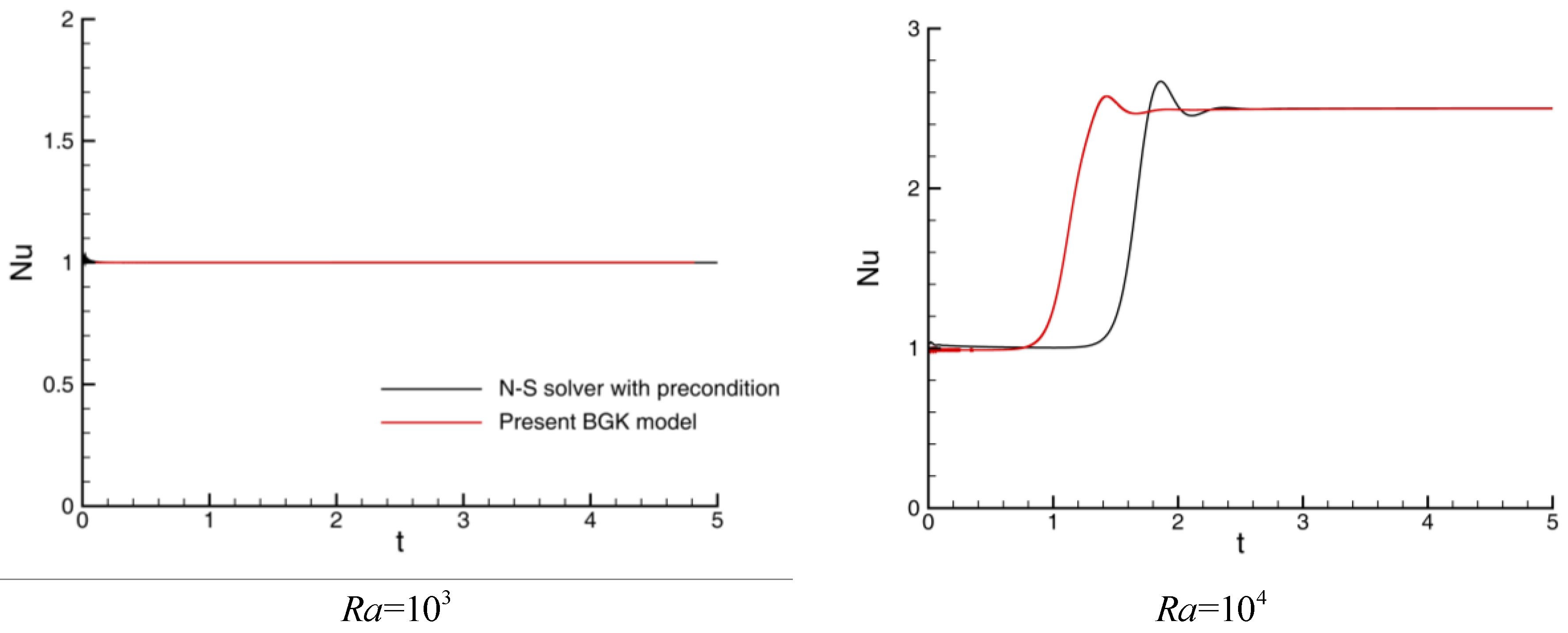
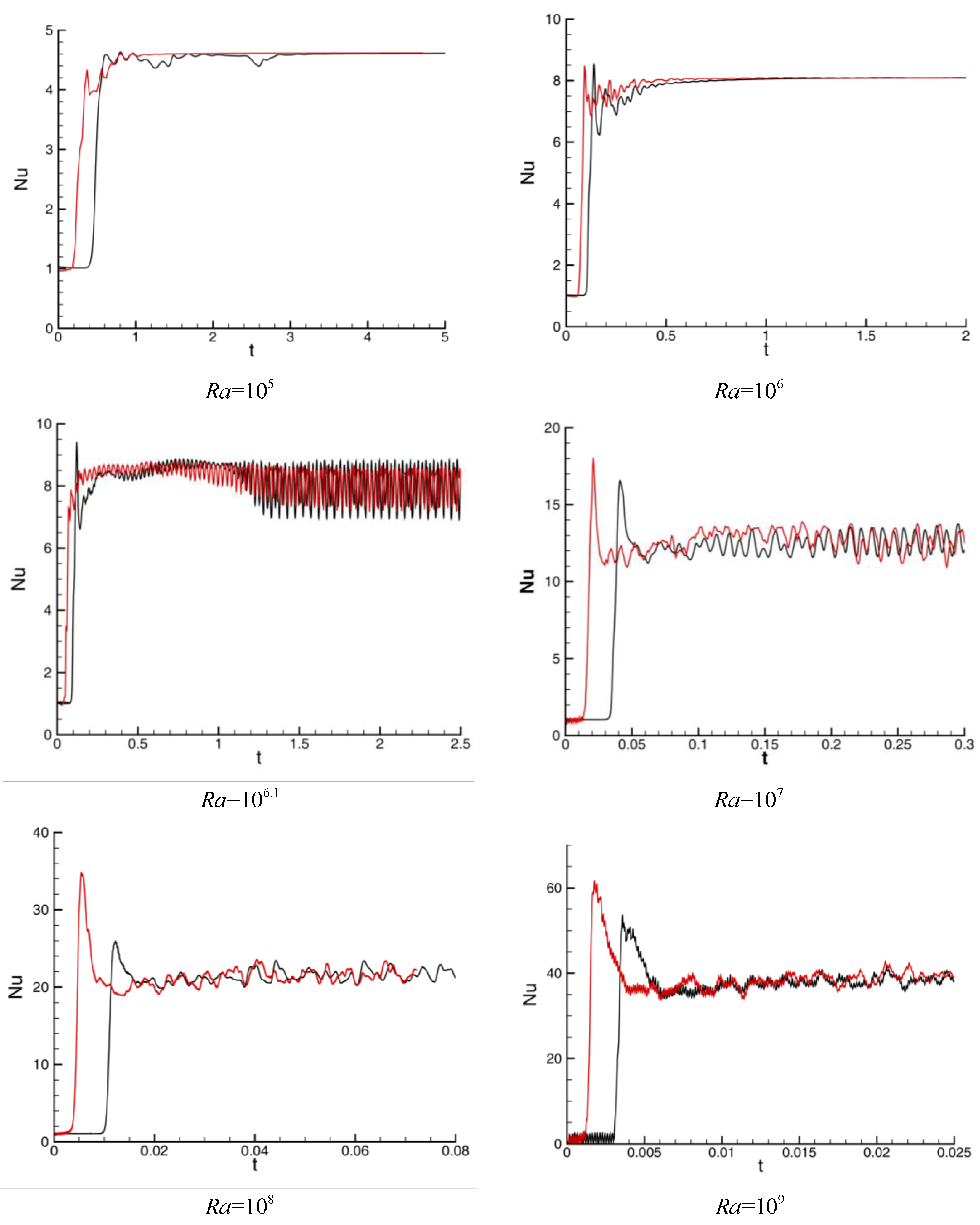
3.2. Nusselt Numbers

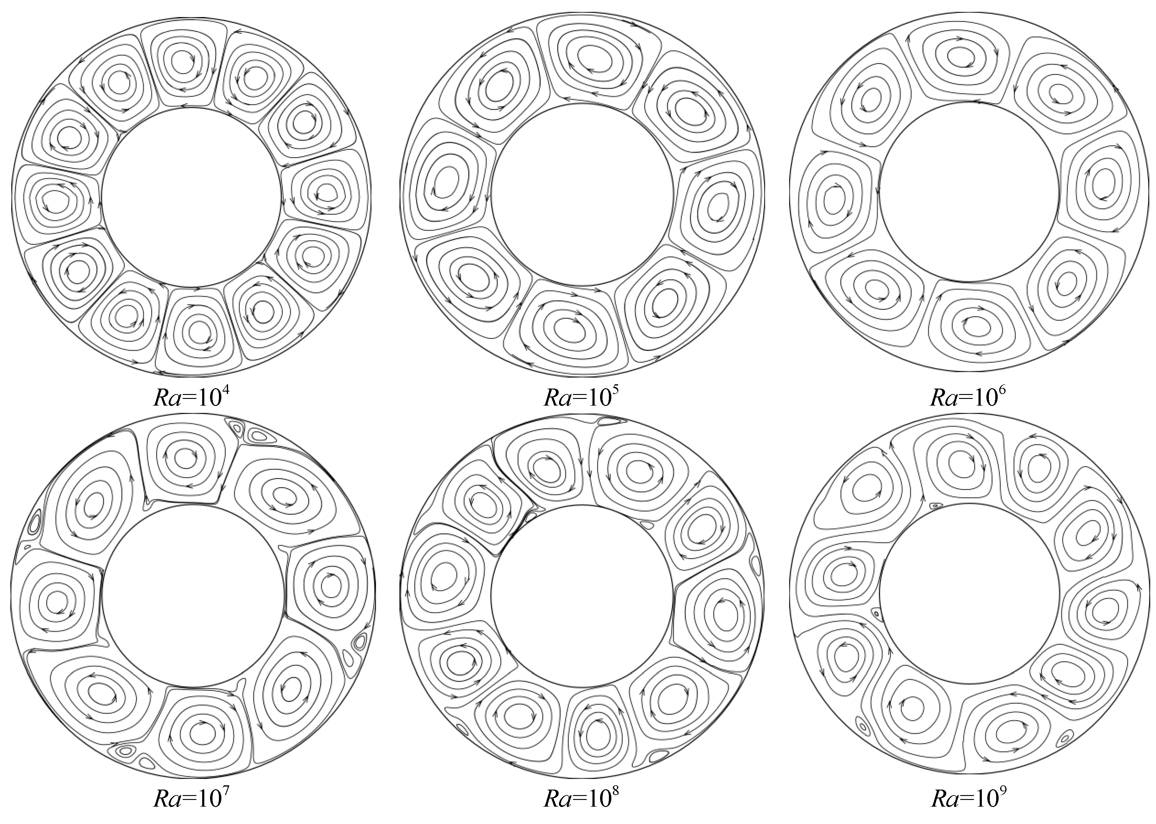
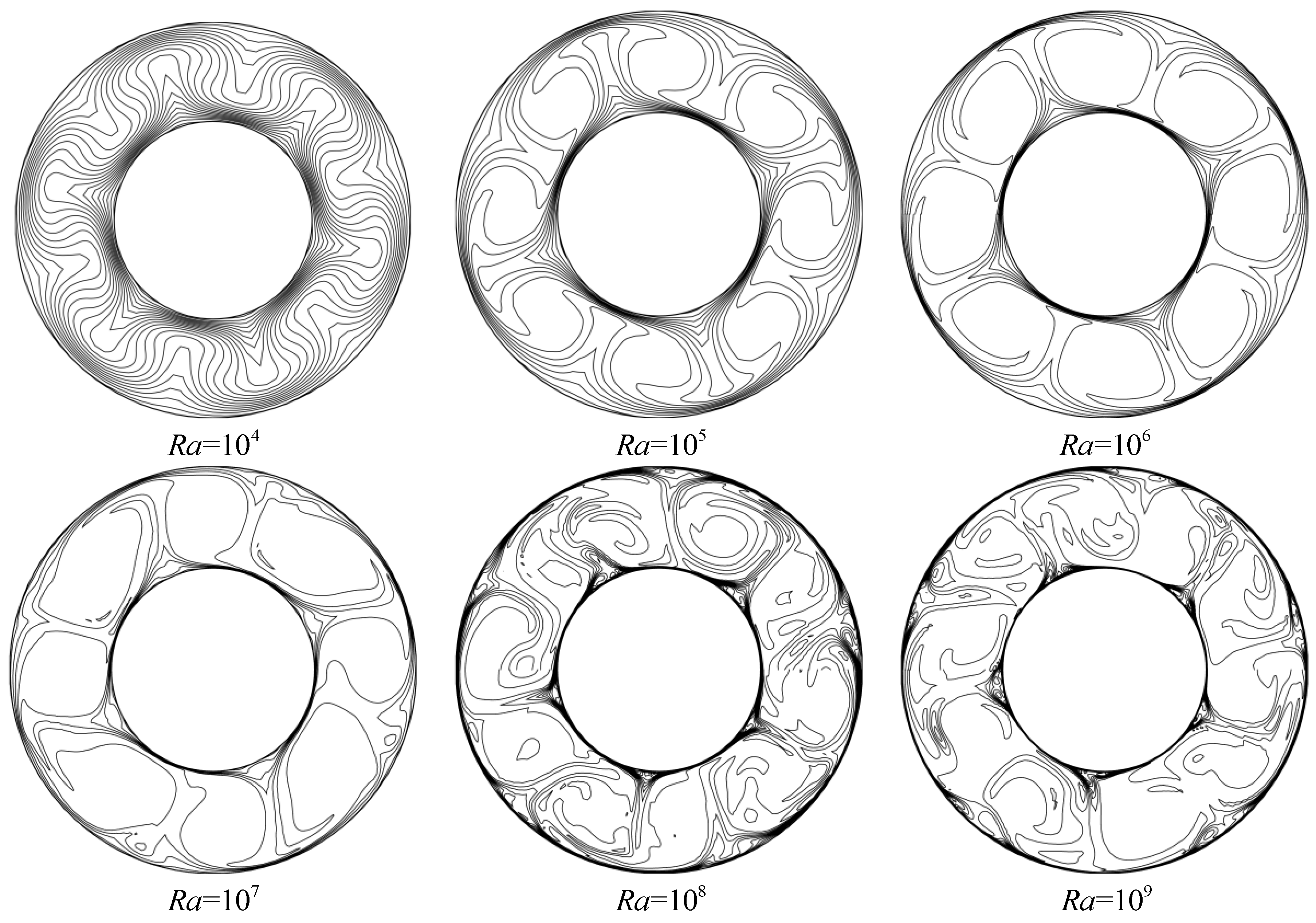
In heat transfer problems, the Nusselt number is an important dimensionless parameter to measure the intensity of convection, which is defined as the ratio of the total heat transfer rate to that due to conduction alone. According to Equation (29), the local Nusselt number $N{u}_{local}$ at the hot (outer) wall is given by

$$N{u}_{local}=\frac{-k{\left(\frac{\partial T}{\partial r}\right)}_{r=r_o}}{-k{\left(\frac{\partial T_{cond}}{\partial r}\right)}_{r=r_o}}=\frac{\ln (r_o/r_i)r_o}{T_h-T_c}{\left(\frac{\partial T}{\partial r}\right)}_{r=r_o},$$

(30)

where the temperature gradient is calculated using a simple finite difference approximation. The global Nusselt number $Nu$ can be obtained by integrating $N{u}_{local}$ over the cylinder surface, which gives

$$Nu=\frac{1}{2\pi }{\displaystyle {\int }_0^{2\pi }\frac{\ln (2)r_o}{T_h-T_c}{\left(\frac{\partial T}{\partial r}\right)}_{r=r_o}d\theta }.$$

(31)

Figure 3 shows the computed variations of $Nu$ with time $t$ at different Rayleigh numbers. Also presented are the results from the N–S solver. It is observed that for $Ra\ge {10}^4$ a convective flow has been developed from the initial pure conduction and pure rotating flow, since all the predicted Nusselt numbers are reaching final values larger than 1 after a short transition process. The convective flow can be seen more clearly from the flow patterns shown in the next section. In fact, the critical value of $Ra$ for this rotating annulus case is between ${10}^{3.2}$ and ${10}^{3.3}$, which is close to the value of 1708 for the Rayleigh–Bénard convection between horizontal plates.

It is also observed from Figure 3 that both numerical methods predict a time-independent $Nu$ for $Ra\le {10}^6$ and a time-dependent one for $Ra\ge {10}^{6.1}$. This transition range is very close to the result of King et al. [4]. For each case with $Ra\le {10}^6$, the converged Nusselt numbers from the two methods agree well with each other, and for each case with $Ra\ge {10}^{6.1}$, the computed time-averaged values show also good agreement. Particularly, approximately periodic oscillations occur for $Ra={10}^{6.1}$ and $Ra={10}^7$, and the oscillations change to irregular states for $Ra\ge {10}^8$. Although the computations started from the same initial condition, the predicted convective flow from the BGK scheme seems to develop earlier.

Figure 4 shows the computed variation of (time-averaged) $Nu$ with $Ra$, together with those from literatures. Note that the computed results from the BGK scheme and the N–S solver are very close to each other. For clarity, we only show the results from the BGK scheme, and their consistency can be clearly seen in Figure 3 (time-independent values for $Ra\le {10}^6$ and time-averaged values for $Ra>{10}^{6.1}$). This indicates that, for the current rotating annulus case, the accuracy of the BGK scheme is comparable to that of the N–S solver; both are based on the full compressible N–S equations. However, when comparing the present results (from both methods) with that from King et al. [6] by using an incompressible solver with the Boussinesq approximation, obvious discrepancies are found for $Ra>{10}^{6.5}$. Currently, these discrepancies are not fully understood. As far as the authors are concerned, besides the numerical reasons, the density effect can be a possible physical reason. As we all know, the density is treated as a constant in the Boussinesq approximation-based solver, while in the current flow solvers, the density is calculated from the ideal gas law. For small $Ra$, the velocity and kinetic energy are small, thus very little difference is found. However, with the increase of $Ra$, the compressible effect may become more and more important. The semi-empirical correlation from Hollands et al. [24] for Rayleigh–Bénard convection is also shown in Figure 4 for comparison. Both the present and King’s results are found to deviate from it at higher $Ra$, and the former predicts lower Nusselt numbers while the latter overpredicts the values

3.3. Flow Pattern

It has been shown from the above numerical results that a steady-state flow field can be obtained for $Ra\le {10}^6$ and the convective flow becomes unstable for $Ra\ge {10}^{6.1}$. Figure 5 and Figure 6 show the streamlines (based on relative velocities) and temperature contours, respectively. For $Ra\le {10}^6$, they do not change with time, while for $Ra\ge {10}^{6.1}$, they are obtained at a certain time, i.e., at $t=2$ for $Ra={10}^7$, at $t=0.05$ for $Ra={10}^8$ and at $t=0.02$ for $Ra={10}^9$.

As shown in Figure 5, several cyclonic and anti-cyclonic pairs of vortices (convective roll pairs) are observed in the rotating cavity, which is similar to the Rayleigh–Bénard convection in a stationary, horizontal enclosure. The number of these vortex pairs not only varies with $Ra$, but also varies with time at higher $Ra$. This irregular number is changing within the range of 4 to 6, which is same as the observation in [6]. With the increase of $Ra$, the convective rolls become more distinguished from each other and the symmetry of the flow structure is broken. Also for $Ra\ge {10}^7$, extra secondary vortices are found among the primary rolls, occurring as a result of flow instability.

As for the temperature contours shown in Figure 6, similar thermal roll pairs start to appear at $Ra={10}^5$ and gradually break down at $Ra={10}^8$. The number of these pairs is equal to that of convective roll pairs for each $Ra$. When $Ra$ is higher than ${10}^8$, the thermal mixing is obvious, leading to chaos thermal structures. It is argued that the flow vacillation should be responsible for the lack of coherence in the temperature contours.

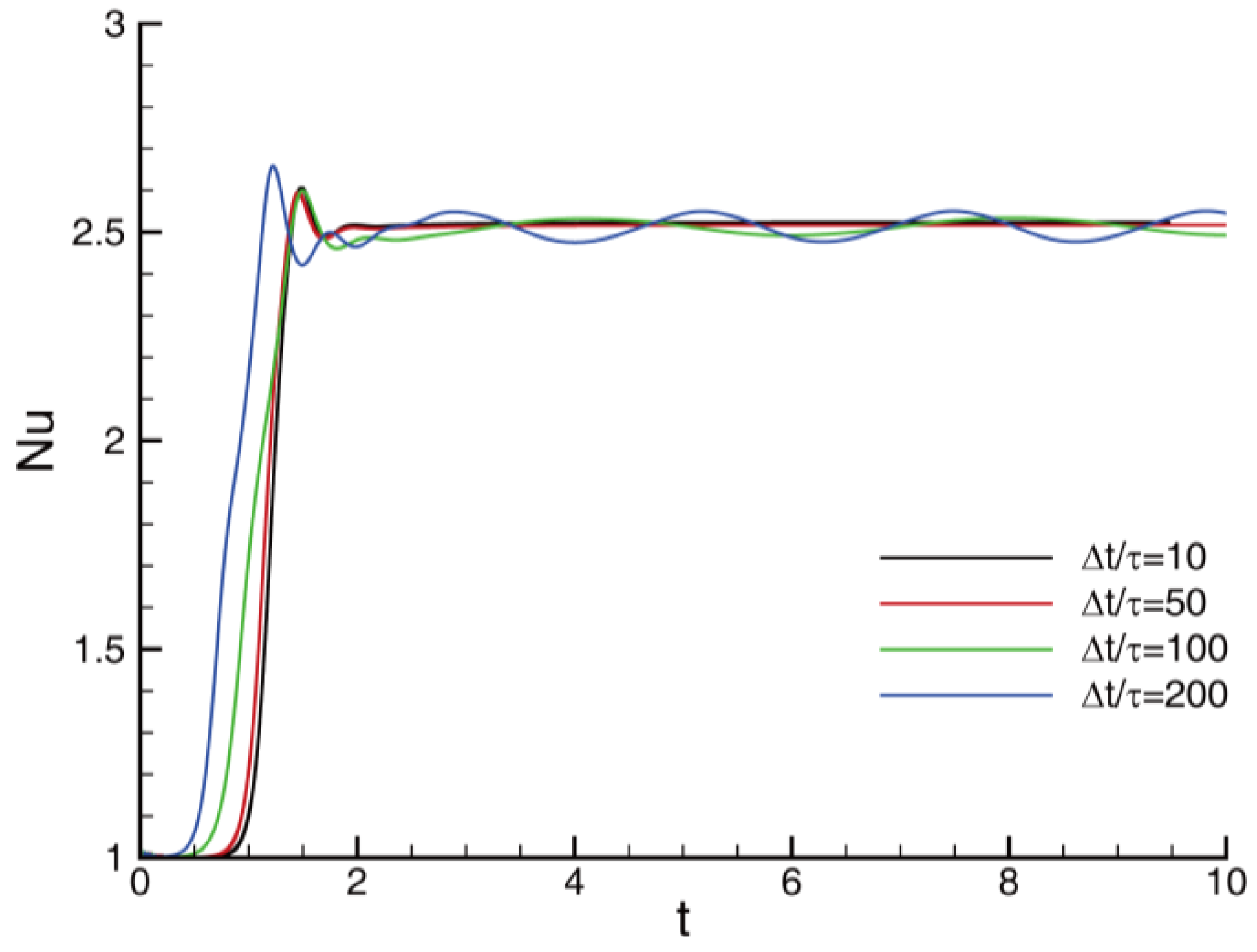
3.4. Effect of Step Size $\Delta t$

Different from the used N–S solver where the (physical) time step size is not a sensitive parameter to affect the simulation results, in the BGK scheme $\Delta t$ needs to be carefully determined. A direct reason is that $\Delta t$ and $\tau =\mu /p$ are decoupled in the BGK scheme, but $\Delta t$ only and the ratio between them are involved in the evaluations of time-dependent distribute function $f$ and fluxes $F$ as shown in Equations (24) and (25). Physically, it is required that $\Delta t/\tau$ should be within a reasonable range in order to correctly reflect the physical reality. For the low-speed viscous flow, sufficient particle collisions $\Delta t$ occur at the cell interface and thus $\Delta t$ should be greatly larger than $\tau$. However, a too large $\Delta t$ could lead to violation of the stability condition. On the other hand, a small $\Delta t$ may decrease the computational efficiency and even implies rarefied flow, where the present Maxwellian-based BGK scheme no longer works. In Xu’s work for Rayleigh–Bénard simulation [16], they kept the collision time $\tau$ to be around ${10}^{-1}\Delta t$. Su et al. [11] suggested that $\Delta t/\tau$ is about 10~100 for any practical simulations.

To clearly show the effect of $\Delta t$ on the simulation result, we study the steady-state case with $Ra={10}^4$ by using four different step sizes corresponding to the ratio $\Delta t/\tau$ of 10, 50, 100 and 200. As shown in Figure 7, for $\Delta t/\tau =10$ and 50, a stable $Nu$ is obtained equaling to 2.5019 and 2.5131, respectively. The difference between them is about 0.2%. But, for $\Delta t/\tau =100$, a periodic oscillation appears and it seems not to decay with time. Although its time-averaged value still agrees well with the previous stable values, this oscillation is physically not true. When $\Delta t/\tau =200$ is used, a more intensive oscillation is found with the larger amplitude and higher frequency, which provides further evidence that the “fake” oscillation is entirely due to the numerics. Therefore it is concluded that when using the present BGK scheme for such low-speed thermal flows, $\Delta t$ cannot be chosen as large as for subsonic/transonic flows. The current used step size $\Delta t=1\times {10}^{-7}$ leads to the value of $\Delta t/\tau \approx 50$, which is a suitable choice.

4. Conclusions

The accuracy of the developed BGK scheme has been proven to be at least as high as that of the conventional preconditioned N–S solver. No preconditioning is required in the BGK scheme, while without it the original N–S solver cannot give reasonable results or even produces floating errors. This corroborates the delicate dissipation mechanism in the BGK scheme for low-speed thermal flows. Besides, the computational effort for each time step is also reduced by more than one-third as compared with the N–S solver. There are mainly two reasons. One is that the preconditioning significantly increases the computational cost for unsteady flows due to the necessity to employ a dual-time stepping approach. Another reason is that the BGK scheme is a single-stage method and less calculation is required for the flux evaluation. However, due to the small step size $\Delta t$ used in the BGK scheme, more computational time steps are needed in order to gain a complete time history of the Nusselt number $Nu$; for example, in this case, the number of time steps needed is four times that of the N–S solver. Therefore, in terms of the total CPU time cost, the current method shows a slight deficiency. In fact, as compared with regular incompressible solvers, both methods can be less efficient for low-speed flows, which are not well resolved. But for the rotating annulus in practical high-speed engines, there exist situations where the compressibility effects cannot be ignored, for example, when a larger temperature difference is encountered or when the forced convection with a higher inlet flow rate is considered. For these cases, the incompressible solvers may suffer from accuracy degradation, while the present BGK scheme still works.

Currently, the turbulence effect is not modeled, which limits the scope of the Rayleigh number. In order to simulate more practical natural convection with a higher Rayleigh number, relevant work is being conducted. Also, as demonstrated previously, the used approach, by replacing the general acceleration term with a simple form of the source term, has its limitations, e.g., it may not be suitable for non-equilibrium flows or other complex flows [25]. This also leaves us much room for a follow-up study.

References

1. Childs, P.R.N. Introduction to rotating flow. In Rotating Flow; Butterworth-Heinemann: Oxford, UK, 2011. [Google Scholar]
2. Bohn, D.; Emunds, R.; Gorzelitz, V.; Krüger, U. Experimental and theoretical investigations of heat transfer in closed gas-filled rotating annuli II. In Proceedings of the ASME 1994 International Gas Turbine and Aeroengine Congress and Exposition, The Hague, The Netherlands, 13–16 June 1994; Volume 4, p. V004T009A027. [Google Scholar]
3. Bohn, D.; Deuker, E.; Emunds, R.; Gorzelitz, V. Experimental and theoretical investigations of heat transfer in closed gas-filled rotating annuli. J. Turbomach. 1995, 117, 175–183. [Google Scholar] [CrossRef]
4. King, M.P. Convective Heat Transfer in a Rotating Annulus; University of Bath: Bath, UK, 2002. [Google Scholar]
5. Bohn, D.; Dibelius, G.H.; Deuker, E.; Emunds, R. Flow pattern and heat transfer in a closed rotating annulus. J. Turbomach. 1994, 116, 542–547. [Google Scholar] [CrossRef]
6. King, M.P.; Wilson, M.; Owen, J.M. Rayleigh-bénard convection in open and closed rotating cavities. J. Eng. Gas Turbines Power 2007, 129, 305–311. [Google Scholar] [CrossRef]
7. Hasan, N.; Sanghi, S. The dynamics of two-dimensional buoyancy driven convection in a horizontal rotating cylinder. J. Heat Transf. 2005, 126, 963–984. [Google Scholar] [CrossRef]
8. Hasan, N.; Sanghi, S. On the role of coriolis force in a two-dimensional thermally driven flow in a rotating enclosure. J. Heat Transf. 2006, 129, 179–187. [Google Scholar] [CrossRef]
9. Sun, Z.; Kifoil, A.; Chew, J.W.; Hills, N.J. Numerical simulation of natural convection in stationary and rotating cavities. In Proceedings of the ASME Turbo Expo 2004: Power for Land, Sea, and Air, Vienna, Austria, 14–17 June 2004; Volume 4, pp. 381–389. [Google Scholar]
10. Michael Owen, J.; Long, C.A. Review of buoyancy-induced flow in rotating cavities. J. Turbomach. 2015, 137, 111001–111013. [Google Scholar] [CrossRef]
11. Su, M.; Xu, K.; Ghidaoui, M.S. Low-speed flow simulation by the gas-kinetic scheme. J. Comput. Phys. 1999, 150, 17–39. [Google Scholar] [CrossRef]
12. Xu, K.; He, X. Lattice boltzmann method and gas-kinetic bgk scheme in the low-mach number viscous flow simulations. J. Comput. Phys. 2003, 190, 100–117. [Google Scholar] [CrossRef]
13. Jin, C.; Xu, K.; Chen, S. A three dimensional gas-kinetic scheme with moving mesh for low-speed viscous flow computations. Adv. Appl. Math. Mech. 2010, 2, 746–762. [Google Scholar]
14. Prendergast, K.H.; Xu, K. Numerical hydrodynamics from gas-kinetic theory. J. Comput. Phys. 1993, 109, 53–66. [Google Scholar] [CrossRef]
15. Xu, K. Gas-Kinetic Schemes for Unsteady Compressible Flow Simulations; Lecture Series; van Kareman Institute for Fluid Dynamics: Rhode-Saint-Genese, Belgium, 1998; Volume 3. [Google Scholar]
16. Xu, K.; Lui, S.H. Rayleigh-bénard simulation using the gas-kinetic bhatnagar-gross-krook scheme in the incompressible limit. Phys. Rev. E 1999, 60, 464. [Google Scholar] [CrossRef]
17. Tian, C.T.; Xu, K.; Chan, K.L.; Deng, L.C. A three-dimensional multidimensional gas-kinetic scheme for the navier–stokes equations under gravitational fields. J. Comput. Phys. 2007, 226, 2003–2027. [Google Scholar] [CrossRef]
18. Wang, P.; Tao, S.; Guo, Z. A coupled discrete unified gas-kinetic scheme for boussinesq flows. Comput. Fluids 2015, 120, 70–81. [Google Scholar] [CrossRef]
19. Wang, P.; Zhang, Y.; Guo, Z. Numerical study of three-dimensional natural convection in a cubical cavity at high rayleigh numbers. Int. J. Heat Mass Transf. 2017, 113, 217–228. [Google Scholar] [CrossRef]
20. Zhou, D.; Lu, Z.L.; Guo, T.Q. Development of a moving reference frame-based gas-kinetic bgk scheme for viscous flows around arbitrarily moving bodies. J. Comput. Phys. 2018. under review. [Google Scholar]
21. Xu, K. A gas-kinetic scheme for the euler equations with heat transfer. SIAM J. Sci. Comput. 1999, 20, 1317–1335. [Google Scholar] [CrossRef]
22. Blazek, J.Z. Structured finite volume schemes. In Computational Fluid Dynamics: Principles and Applications, 2nd ed.; Elsevier Science: Amsterdam, The Netherlands, 2005; pp. 210–213. [Google Scholar]
23. Xu, K. A gas-kinetic bgk scheme for the navier–stokes equations and its connection with artificial dissipation and godunov method. J. Comput. Phys. 2001, 171, 289–335. [Google Scholar] [CrossRef]
24. Hollands, K.G.T.; Raithby, G.D.; Konicek, L. Corrrelation equations for free convection heat transfer in horizontal layers of air and water. Int. J. Heat Mass Transf. 1975, 18, 879–884. [Google Scholar] [CrossRef]
25. Balescu, R. Neoclassical Tarnsport Theory. In Transport Processes in Plasmas; North-Holland Publishing Company: Amsterdam, The Netherlands, 1988; Volume 2. [Google Scholar]
Figure 1. Radial distributions of (a) circumferential velocity v c ; (b) pressure gradient p / r for the rotating Couette case.
Applsci 08 00733 g001
Figure 2. Radial distributions of temperature T for the pure conduction case.
Applsci 08 00733 g002
Figure 3. Computed variations of N u with time t for different R a .
Applsci 08 00733 g003aApplsci 08 00733 g003b
Figure 4. Comparison of computed variations of (time-averaged) N u with R a .
Applsci 08 00733 g004
Figure 5. Computed instantaneous streamlines for different R a .
Applsci 08 00733 g005
Figure 6. Computed instantaneous temperature contours for different R a .
Applsci 08 00733 g006
Figure 7. The effect of step size Δ t on variation of N u with time t for R a = 10 4 .
Applsci 08 00733 g007