Proposing Enhanced Feature Engineering and a Selection Model for Machine Learning Processes

Featured Application

This module can be used independently in any Machine Learning project or can be used in a model that is engineered by boosting and blending of algorithms for better accuracy and fitness.

Abstract

Machine Learning (ML) requires a certain number of features (i.e., attributes) to train the model. One of the main challenges is to determine the right number and the type of such features out of the given dataset’s attributes. It is not uncommon for the ML process to use dataset of available features without computing the predictive value of each. Such an approach makes the process vulnerable to overfit, predictive errors, bias, and poor generalization. Each feature in the dataset has either a unique predictive value, redundant, or irrelevant value. However, the key to better accuracy and fitting for ML is to identify the optimum set (i.e., grouping) of the right feature set with the finest matching of the feature’s value. This paper proposes a novel approach to enhance the Feature Engineering and Selection (eFES) Optimization process in ML. eFES is built using a unique scheme to regulate error bounds and parallelize the addition and removal of a feature during training. eFES also invents local gain (LG) and global gain (GG) functions using 3D visualizing techniques to assist the feature grouping function (FGF). FGF scores and optimizes the participating feature, so the ML process can evolve into deciding which features to accept or reject for improved generalization of the model. To support the proposed model, this paper presents mathematical models, illustrations, algorithms, and experimental results. Miscellaneous datasets are used to validate the model building process in Python, C#, and R languages. Results show the promising state of eFES as compared to the traditional feature selection process.

1. Introduction

One of the most important research directions of Machine Learning (ML) is Feature Optimization (FO) (collectively grouped as Feature Engineering (FE), Feature Selection (FS), and Filtering) [1]. For FS, a saying “Less is More” becomes the essence of this research. Dimensionality Reduction [2] has become a focus in the ML process to avoid unnecessary computing power/cost, overlearning, and predictive errors. In this regard, redundant features which may have similar predictive value to other feature(s), may be excluded without negatively affecting the learning process. Similarly, the irrelevant features should be excluded as well. FS and FE not only focuses on extracting a subset from the optimal feature set but also building new feature sets previously overlooked by ML techniques. This also includes reducing the higher dimensions into lower ones to extract the feature’s value. Latest research has shown noteworthy progress in FE. In [3], the authors reviewed the latest progress in FS and associated algorithms. Out of a few, principal component analysis (PCA) [4] and Karhunen Loeve expansion [5] are widely used with eigen-values and eigen-vectors of the data covariance matrix for FO. The squared error is calculated as well in the mapping of orthonormal transformation to reduce general errors. Another approach is Bayes error probability [6] to evaluate a feature set. However, Bayes errors are generally unknown. Discriminant analysis are also used in FE. Hence, in the line with the latest progress and related study (See Section 2), the work proposed in this paper uses ML and mathematical techniques, such as statistical pattern classification [7], Orthonormalization [8], Probability theory [9], Jacobian [7], Laplacian [3], and Lagrangian distribution [10] to build the mathematical constructs and underlying algorithms (1 and 2). To advance such developments, a unique engineering of the features is proposed where the classifier learns to group an optimum set of features without consuming excessive computing power, regardless of the anatomy of the underlying datasets and predictive goals. This work also effectively addresses the known challenges of ML process such as overfitting, underfitting, predictive errors, poor generalization, and low accuracy.

1.1. Background and Motivation

Despite using the best models and algorithms, FO is crucial to the performance of the ML process and predictions. FS has been a focus in the fields of data mining [11], data discovery, text classification [12], and image processing [13]. Unfortunately, raw datasets pose no clear advice or insight into which variables must be focused on. Usually, datasets contain several variables/features but not all of them contribute towards predictive modeling. Another significance of such research is to determine the intra- and inter-relationships between the features. Their internal dependence and correlation/relevance greatly impact the way a model learns from the data. To make the process computationally inexpensive and keep the accuracy higher, features should be categorized by the algorithm itself. The existing literature proves that such work is rarely undertaken in ML research.

1.2. Parent Research

The proposed model eFES is a participating module of the enhanced machine learning engine engineering (eMLEE) model, which is based on parallel processing and learns from its mistakes (i.e., processing and storing the wrong predictions). Other than eFES, the rest of the four modules as shown in Figure 1 are beyond the scope of this paper. Specifically, eMLEE modules are: (i) enhanced algorithm blend and tuning (eABT) to optimize the classifier performance; (ii) enhanced feature engineering and selection (eFES) to optimize the features handling; (iii) enhanced weighted performance metric (eWPM) to validate the fitting of the model; and (iv) enhanced cross validation and split (eCVS) to tune the validation process. Out of these, eCVS is in its infancy in the research work. Existing research, as discussed in Section 2, has shown the limitations of general purpose algorithms in Supervised Learning (SL) for predictive analytics, decision making, and data mining. Thus, eFES (i.e., the part of eMLEE) fills the gaps that Section 2 discusses.

1.3. Our Contributions

Our contributions are the following.

• Improved feature search and quantification for unknown or previously unlabeled features in the datasets for new insights and the relevance of predictive modeling.
• Outlier identification to minimize the effects on classifier learning.
• Constructing a feature grouping function (FGF) to add or remove a feature once we have scored them in their correlation, relevance, and non-redundancy nature of predictive value. Identifying the true nature of the feature vs attribute so bias can be reduced. Features tend to gain or lose their significance (predictive value) from one dataset to another. A perfect example would be an attribute “Gender” (e.g., Gender/Sex may not have any predictive value in a certain type of the dataset/prediction). However, it may have significant value in the different dataset.
• Constructing a logical 3D space where each feature is observed for its fitness value. Each feature can be quantified based on a logical point in 3D space. Its contribution towards overfitting (x), underfitting (y), and optimum-fitting (z) can be scored, recorded, and then weighted for adding or removing in FGF.
• Developing a unique approach of utilizing an important metric in ML (i.e., error). We have trained our model to be governed by maximum and minimum bounds of the error, so we can maintain acceptable bias and fitness including overlearning. Our maximum and minimum bounds for errors are 80% and 20% respectively. These error bounds can be considered one of our novel ideas in the proposed work. The logic goes thus: models are prone to overfitting, bias, high errors, and low accuracy. We tried to envision if the proposed model can be governed by some limits of the errors. Errors above 80% or below 20% are considered red flags. Such may indicate, bias, overlearning or under-learning of the model. Picking 80% and 20% was our rule of thumb to validate our theory with experiments on a diverse dataset (discussed in the appendix).
• Finally, engineering local gain (LG) and global gain (GG) functions to improve the feature tuning and optimization.

Figure 2 shows the elevated level block diagram of the eFES Unit.

2. Related Study

To identify the gaps in the latest state of the art in the field of FO, we considered area of ML where FO was of high relevance. In general, every ML problem is affected by feature selection and feature processing. Predictive modeling, as our focus for the consumption of the proposed model, is a great candidate to be looked at, for FO opportunities. One of the challenges in FO is to mine the hidden features that are previously unknown and may hide a great predictive value. If such knowledge can be extracted and quantified, ML process can dramatically be improved. On the other hand, new features can also be created by aggregating existing features. Also, two irrelevant features can be combined, and their weighted function can become a productive feature with higher predictive value. Clearly, in-depth comprehensive review of the FO and related state of the art are outside the scope of this paper. However, in this section we provide the related study of noteworthy references and then list the gaps we identified. We also present the comparisons of some of the techniques in Section 5.

Li et al. [3] presented a detailed review of the latest development in the feature selection segment of machine learning. They provided various frameworks, methods, and comparisons in both Supervised Learning (SL) and Unsupervised Learning (UL). However, their comparative study did not reveal any development where each feature can achieve a run-time predictive scoring and can be added or removed algorithmically as the learning process continues. Vergara and Estevez [14] reviewed feature selection methods. They presented updates on results in a unifying framework to retrofit successful heuristic criteria. The goal was to justify the need of the feature selection problem in depth concepts of relevance and redundancy. However, their work was only focused on unifying frameworks and placed the generalization on broader scale. Mohsenzadeh et al. [15] utilized a sparse Bayesian learning approach for feature sample selection. Their proposed relevance sample feature machine (RSFM) is an extension of RVM algorithm. Their results showed the improvement in removing irrelevant features and producing better accuracy in classification. Additionally, their results also demonstrated better generalization, less system complexity, reduced overfitting, and computational cost. However, their work needs to be extended to more SL algorithms. Ma et al. [16] utilized Particle Swarm Optimization (PSO) algorithm to develop their proposed approach for detection of falling elderly people. Their proposed research enhances the selection of variables (such as hidden neurons, input weights, etc.) The experiments showed higher sensitivity, specificity, and accuracy readings. Their work though in the domain of healthcare industry does not address the application of approach to a different industry with an entirely different dataset. Lam et al. [17] proposed a unsupervised feature-learning process to improve the speed and accuracy, using the Unsupervised Feature Learning (UFL) algorithm, and fast radial basis function (RBF) for further feature training. However, the UFL may not fit when applied. SL. Han et al. [18] used circle convolutional restricted Boltzmann machine method for 3D feature learning in unsupervised process of ML. The goal was to learn from raw 3D shapes and to overcome the challenges of irregular vertex topology, orientation ambiguity on the surface, and rigid transformation invariances in shapes. Their work using 3D modeling needs to be extended to SL domains and feature learning. Zeng et al. [19] used the deep perceptual features for traffic sign recognition in the kernel extreme learning machines. Their proposed DP-KELM algorithm showed high efficiency and generalization. However, the proposed algorithm needs to be tested across different traffic systems in the world for more distinctive features than those they have considered. Wang et al. [20] discussed the process of purchase decision in subject minds using MRI scanning images through ML methods. Using the recursive cluster elimination-based SVM method, they obtained higher accuracy (71%) as compared to previous findings. They utilized Filter (GML) and wrapping methods (RCE) for feature selection. Their work also needs to be extended to other image techniques in healthcare. Lara et al. [21] provided a survey on ML application for wearable sensors, based on human activity recognition. They provided a taxonomy of learning approach and their related response time on their experiments. Their work also supported feature extraction as an important phase of ML process. ML has also shown a promising role in engineering, mechanical, and thermo-dynamic systems. Zhang et al. [22] worked on ML techniques to do the prediction in the thermal systems for systems components. Besides many different units and technique adoptions, they also utilized FS methods based on correlation feature selection algorithm. They used Weka data-mining tools and came up with the reduced feature set of 16 for improved accuracy. However, their study did not reveal how exactly they came up with this number and whether different number of the features would have helped any further. Wang et al. [23] used the supervised feature method to remove redundant features and considered the important ones for their gender classification. However, they used the neural network method as a feature extraction method, which is mostly common in unsupervised learning. Their work is yet to be tested for more computer vision tasks including image recognition tasks in which bimodal vein modeling becomes significant. Liu et al. [24] utilized the concept of F-measure optimization for FS. They developed a cost-sensitive feature approach to determine the best F-measure-based feature for the selection by ML process. They argued F-measure to be better than accuracy, for purposes of performance measurement. However, accuracy is not sufficient to be considered a baseline for performance reflection of any model or process. Abbas et al. [25] proposed solutions for IoT-based feature models using the multi-objective optimum approach. They enhanced the binary pattern for nested cardinality constraints using three paths. The second path was observed to increase the time complexity due to the increasing group of features. Though their work was not directly in ML methodologies, their work showed performance improvement in the 3rd path when the optional features were removed.

Here are the gaps that we identified based on a comprehensive literature review and comparisons made, evaluated, and presented in Section 5 later in this paper.

• Parallel processing of the features, in which features can be evaluated one by one, has not been done, while the model metrics are being measured and recorded simultaneously to see the real-time effect.
• Improved grouping of features is needed across diverse feature types in datasets for improved performance and generalization.
• 3D modeling is rarely done. The 3D approach can help for side-by-side metric evaluation.
• Accuracy is taken as granted to measure the performance of the model. However, we argue on the relevance of this metric and support other metrics in conjunction with it. We engineer our model to incline towards the metrics that are found relevant for a given problem based on the classifier learning.
• Feature quantification and function building governed by algorithms the way we presented is not found in the literature, and the dynamic ability of such a design, as our work indicated, can be a good filler of this gap in the state of the art.
• Finally, FO has not been directly addressed. FO helps to regulate the error biasing, outlier detection, and poor generalization.

3. Groundwork of eFES

This section presents background on the underlying theory, mathematical constructs, definitions, algorithms, and the framework.

The elevated-level framework shown in Figure 3 elaborates on the importance of each definition, incorporated with the other units of eMLEE and the ability to implement parallel processing by design. In general computing, parallel processing is done by dividing program instructions to be run by multiple processors, so the time efficiency can be improved. This also ensures the maximum utilization of otherwise idle processors. Similar concepts can be implemented on the algorithms and ML models. ML algorithms depend on the problem and data types and require sequential training of each of the data models. However, the parallel processing can dramatically improve the learning process, especially for the blended model, such as eMLEE. In light of the latest work of parallel processing in ML, such as in [26], the authors introduced the parallel framework on ML algorithms for large graphs. They experimented with aggregation and sequential steps in their model to allow researchers to improve the usage of various algorithms. Another study was done in [27], where authors used induction to improve the parallelism in the decision trees. Python and R libraries have come a long way to help provide useful libraries and classes to develop various ML techniques. Authors in [28] introduced a python library Qjan to parallelize the ML algorithms in compliance by MapReduce. A PhD thesis [29] work done by a student at the University of California at Berkeley used concurrency control method to parallelize the ML process. Another study done in [30] utilized parallel processing approaches in ML techniques for detection in big-data networks. Therefore, similar progresses have motivated us to incorporate parallel processing in the proposed model.

Our proposed model parallelism is done in two layers:

(i)

Outer layer to eFES, where eFES unit communicates with other units of the eMLEE such as eABT, eWPM, eCVS and LT. Parallelism is done through real-time metric measurement with LT object and based on classifier learning, eFES reacts to the inner layer (defined next). Other units such as eABT and eCVS enhance the algorithm blend and test-training split in parallel, while eFES is being trained. In other words, all four units including eFES regulated by LT unit, are run in parallel to improve the speed of the learning process and validation for every feature as processed in the eFES unit and every algorithm processed in the eABT unit. However, eFES can also work without being related to the other units, if researchers and industrialists may however choose so.

(ii)

Inner layer to eFES, where adding and removing of the feature are done in parallel. When the qualifying feature is added, the metrics are measured by the model to see if fitness improves, and then features are added and removed one by one to see the effect on the fitness function. This may be done sequentially, but parallelism improves the insurance that each feature is evaluated at the same time; the classifier is incorporating metrics reading from LT object and speed of the process especially when the huge dataset is being processed.

Figure 3 illustrates the inner layer parallel processing of each construct that constitutes the eFES unit. It shows the high-level block diagram of eFES unit modeling and related functions. Each definition is explained in plain English next.

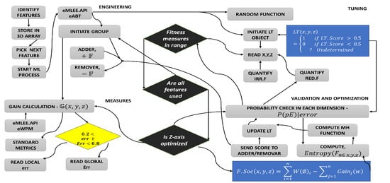
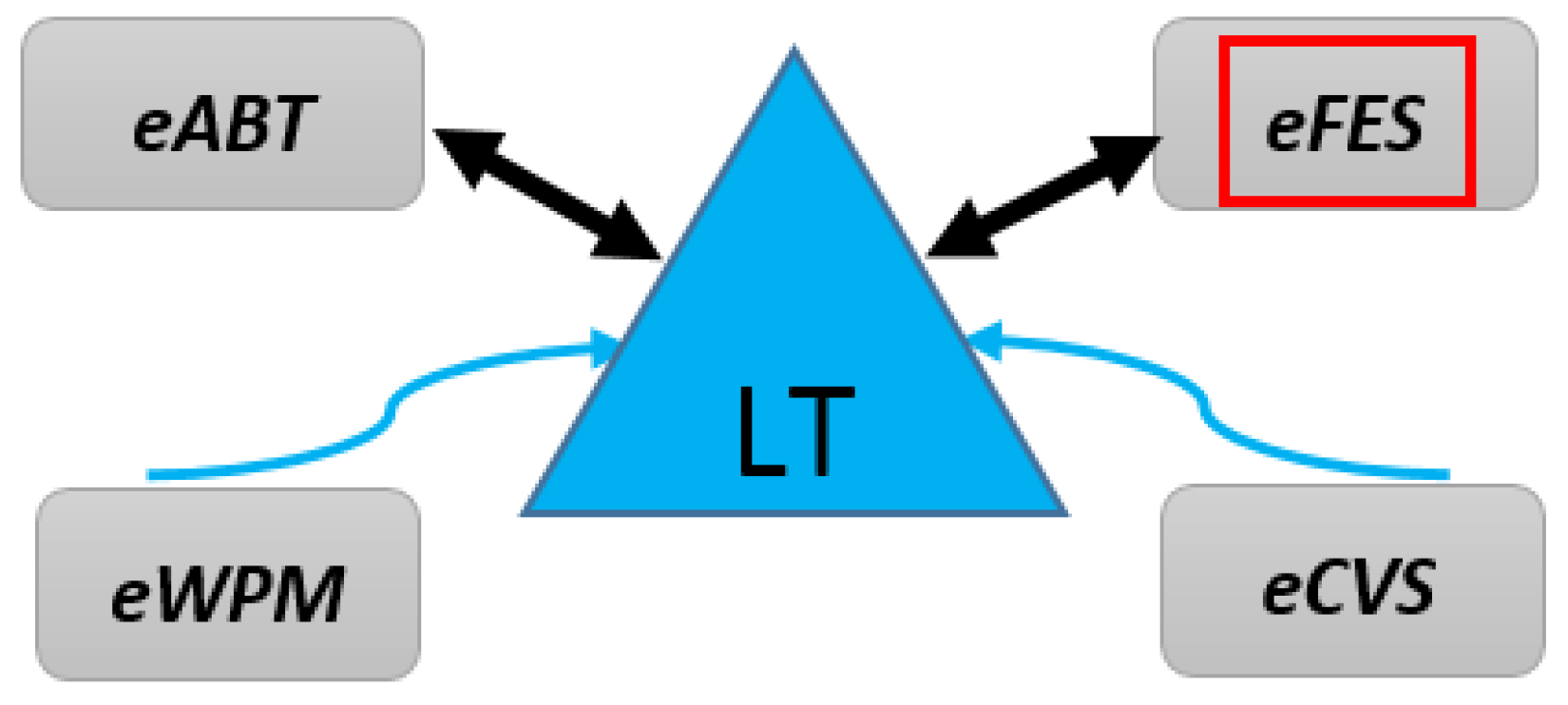
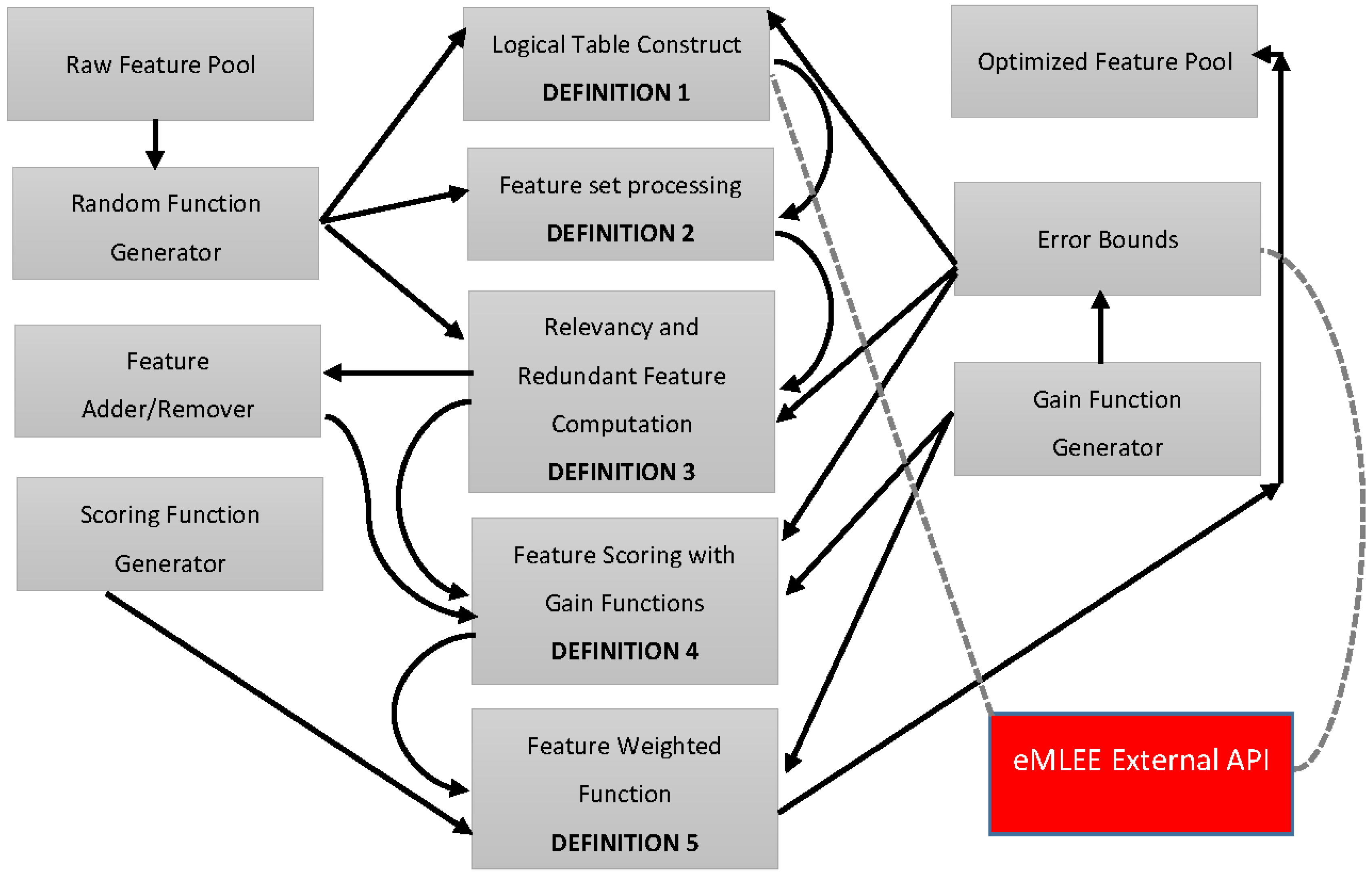
Definition 1 covers the theory of LT unit, which works as a main coordinator assisting and regulating all the sub-units of eMLEE engine such as eFES. It inherently is based on parallel processing at a low level. While the classifier is in the learning process, LT object (in parallel) performs the measurements, records it, updates it as needed, and then feeds the learning process back. During classifier learning, LT object (governed by LT algorithm, outside of scope of this paper, but will be available as an API) creates a logical table (with rows and columns) where it adds or removes the entry of each feature as a weighted function, while constantly measuring the outcome of the classifier learning.

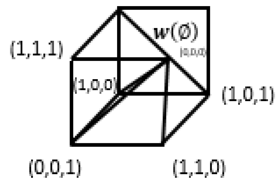
Definition 2 covers the creation of the feature set from raw input via random process, as shown above. As discussed earlier, it uses 3D modeling using x, y, and z coordinates. Each feature is quantized based on the scoring of these coordinates (x being representative of overfit, y being underfit and z being an optimum fit).

Definition 3 covers the core functions of this unit to quantify the scoring of the features, based on their redundancy and irrelevancy. It does this in a unique manner. It should be noted that not every irrelevant feature with high score will be removed by the algorithm. That is the beauty of it. To increase the generalization of such model with a diverse dataset that it has not seen during test (i.e., prediction), features are quantified, and either kept, removed, or put on the waiting list for re-processing of addition or removal evaluation. The benefit of this approach is that it will not do injustice to any feature without giving a second chance later in the learning process. This is because features, once aggregated with a new feature or previously unknown feature, can dramatically improve scores to participate in the learning process. However, the deep work of “unknown feature extraction” is kept for future work, as discussed in the future works section.

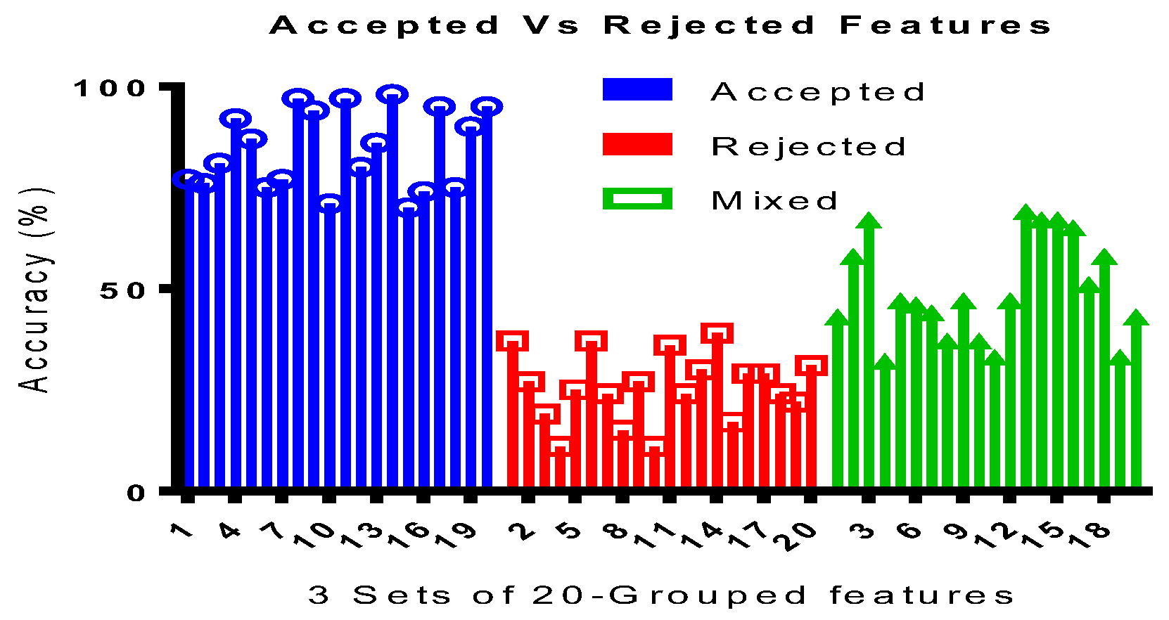
Definition 4 utilizes definition 1 to 3 and introduces a global and local gain functions to evaluate the optimum feature-set. Therefore, the predictor features, accepted features, and rejected features can be scored and processed.

Definition 5 finally covers the weight function to observe the 3D weighted approach for each feature that passes through all the layers, before each feature is finally added to the list of the final participating features.

The rest of the section is dedicated to the theoretical foundation of mathematical constructs and underlying algorithms.

3.1. Theory

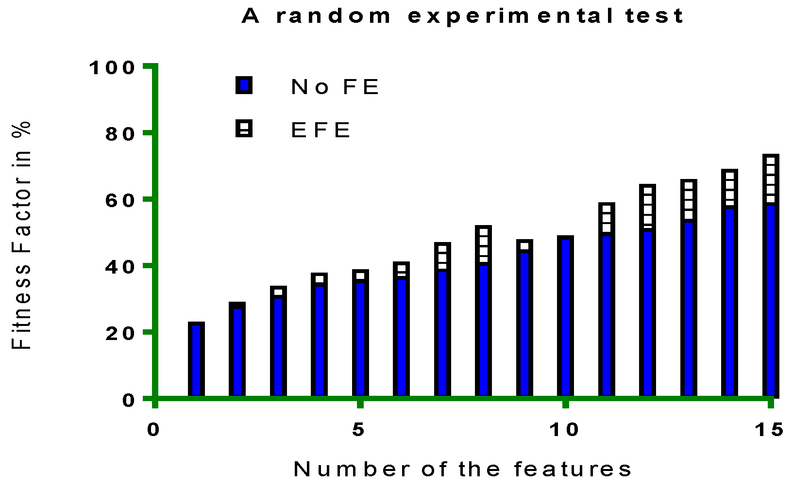
eFES model manifests itself into specialized optimization goals of the features in the datasets. The most crucial step of all is the Extended Feature Engineering (EFE) that we refer when we build upon existing EF techniques. These five definitions help build the technical mechanics of the proposed model of eFES unit.

Definition 1.

Let there be a Logical Table (LT) module that regulates the ML process during eFES constructions. Let LT have 3D coordinates as x, y, and z to track, parallelize, and update the x ← overfit(0:1), y ← underfit(0:1), z ← optimumfit(−1:+1). Let there be two functions, Feature Adder as +𝔽, and Feature Remover as −𝔽, based on linearity of the classifier for each feature under test for which the RoOpF (Rule. 1) is valid. Let Lt. RoOpF > 0.5 to be considered of acceptable predictive value.

eFES LT module builds very important functions at initial layers for adding a good fit feature and removing a bad fit feature from the set of features available to it, especially when algorithm blend is being engineered. Clearly, not all features will have an optimum predictive value and thus identifying them will count towards optimization. The feature adder function is built as:

$$+\mathbb{F}\left(x,y,z\right)=+{\mathbb{F}}_{F_n}= (F_n\cup F_{n+1}) {\displaystyle \sum }_{i=1}^Z\left(LT.score (i\right))+ {{\displaystyle \sum }}_{j,k=1}^{x,y} (LT.score \left(j,k\right))$$

(1)

The feature remover function is built as:

$$-\mathbb{F}\left(x,y,z\right)=-{\mathbb{F}}_{F_n}= (F_n\cap F_{n+1}) {\displaystyle \sum }_{j,k=1}^{x,y}\left(LT.score \left(j,k\right)\right)- {{\displaystyle \sum }}_{i=1}^z \left(LT.score\left(i\right)\right)$$

(2)

Very similar to k-means clustering [12] concept, that is highly used in unsupervised learning, LT implements feature weights mechanism (FWM) so it can report a feature with high relevancy score and non-redundant in a quantized form. Thus, we define:

$$FWM\left(X,Y,Z\right)={\displaystyle \sum }_{x=1}^X{\displaystyle \sum }_{y=1}^Y{\displaystyle \sum }_{z=1}^Z (u_x{w}_x. u_y{w}_y .u_z{w}_z) (\Delta \left(x,y,z\right))$$

(3)

$$\Delta \left(x,y,z\right)= \{\begin{array}{c}{\displaystyle \prod }_{l=1}^L (u_{lx}{w}_{lx}), \mathrm{if} z \ne 0, AND z > \left(0.5, y\right)\\ u_i\in \left\{0,1\right\}, -1 \le i \le L\\ {\displaystyle \prod }_{l=1}^L (u_{ly}{w}_{ly}), \mathrm{if} z \ne 0, AND z > \left(0.5, x\right)\end{array}$$

(4)

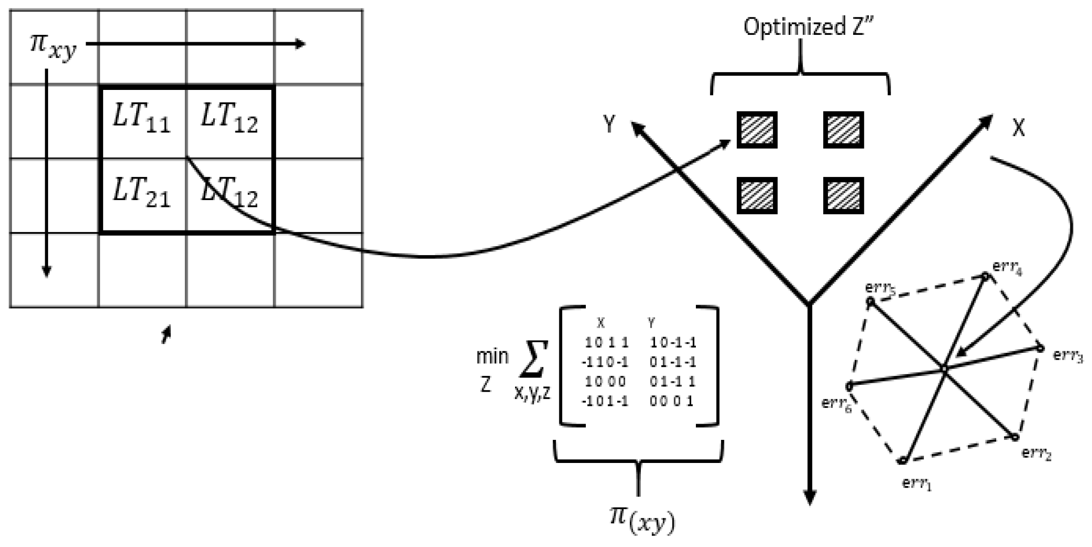
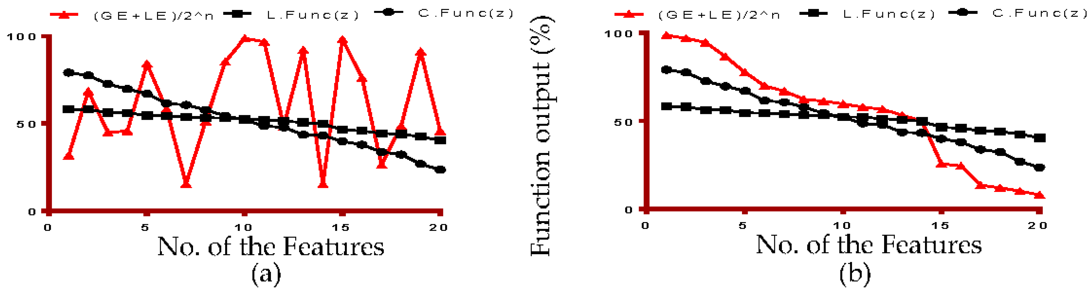
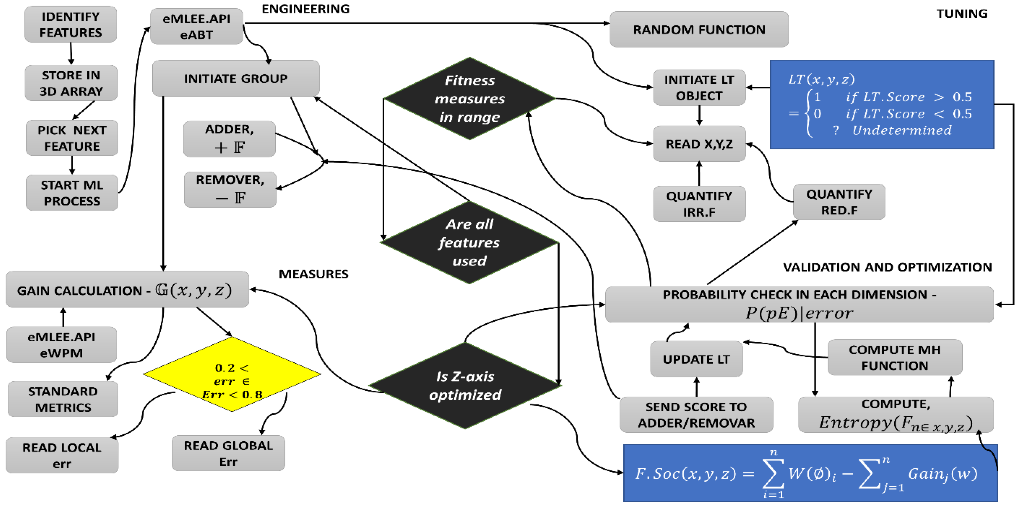
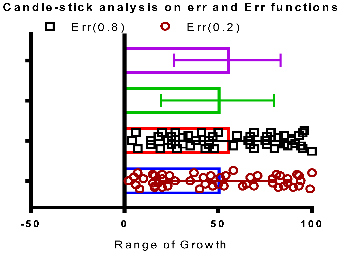
Illustration in Figure 4 shows the concept of LT modular elements in 3D space as discussed earlier. Figure 5 shows the variance of the LT. Figure 6 shows that it is based on binary weighted classification scheme to identify the algorithm for blending and then assign a binary weight accordingly in LT logical blocks. The diamond shape shows the err distribution that is observed and recorded by LT module as new algorithm is added or existing is removed. The complete mathematical model for eFES LT is beyond the scope of this paper. We finally provide the eFES LT functions as:

$$eFE{S}^{⊞}= [{ℝ}_{eFES }= \frac{1}{N_e} {\left(\sqrt{\frac{err}{err + Err}}\right)}^2] \times {\displaystyle \sum }_{n=1}^N{F}_n(f\left(x,y,z\right)\left|exp\left(\frac{+{\mathbb{F}}_{F_n}}{+{\mathbb{F}}_{F_n}+ (-{\mathbb{F}}_{F_n}) }\right)\right|$$

(5)

where err = local error (LE), Err = global error (GE). f (x, y, z) is the main feature set in ‘F’ for 3D.

RULE 1If (LTObject.ScoFunc (A (i) > 0.5) Then
              Assign “1”
        Else Assign “0”
         
        PROCEDURE 1
        Execute LT.ScoreMetrics (Un.F, Ov.F)
        Compute LT.Quantify (*LT)
        Execute LT.Bias (Bias.F, *)
        *_Shows the pointer to the LT object.
		

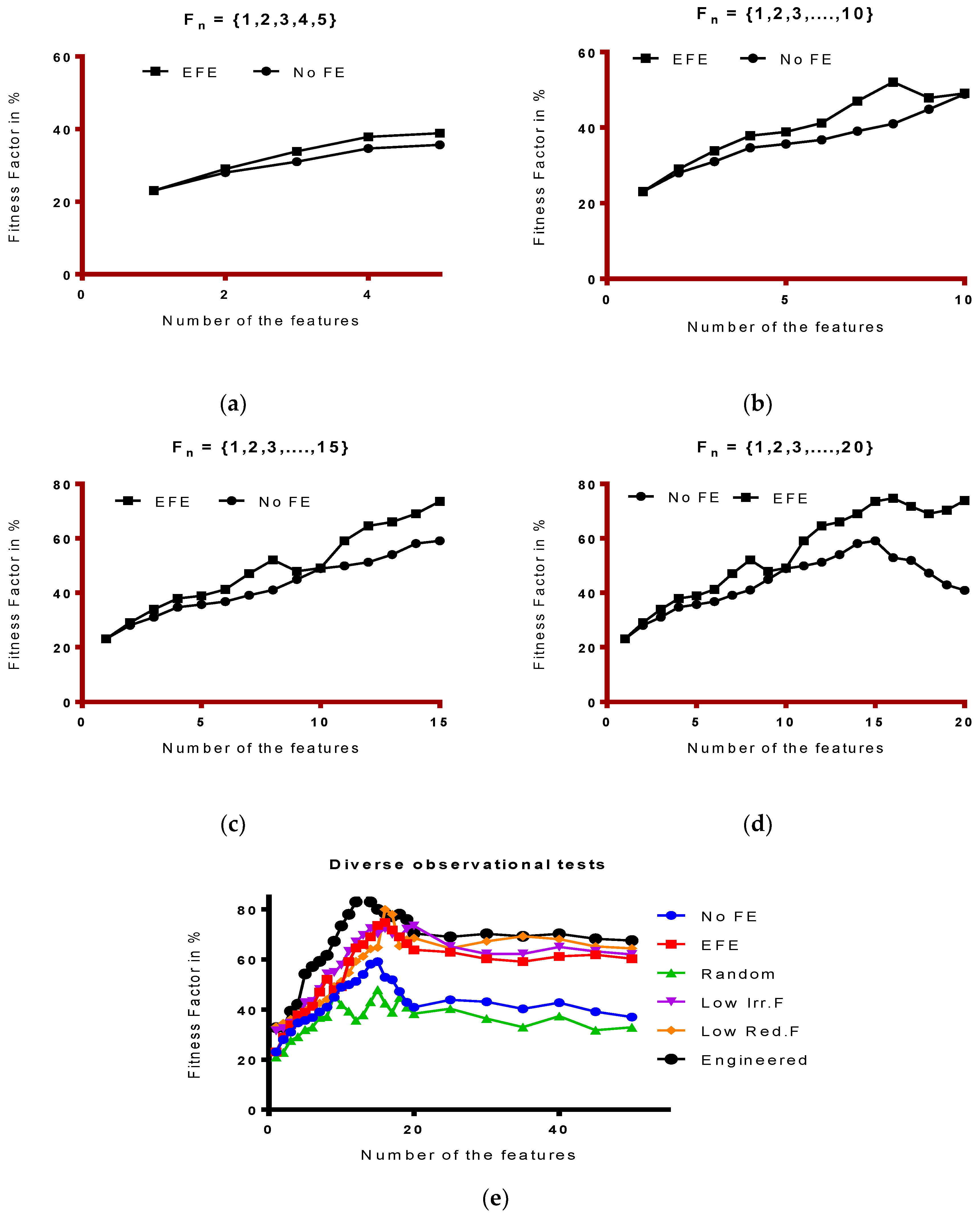
Definition 2.

F_n = {F₁, F₂, F₃, … …, F_n} indicates all the features appears in the dataset, where each feature F_i ∈ F_n|f_w ≥ 0. f_w indicates the weighted feature value in the set. Let F_ran (x,y,z) indicates the randomized feature set.

We estimate the cost function based on randomized functions. Las Vegas and Monte Carlo algorithms are popular randomized algorithms. The key feature of the Las Vegas algorithm is that it will eventually have to make the right solution. The process involved is stochastic (i.e., not deterministic) and thus guarantee the outcome. In case of selecting a function, this means the algorithm must produce the smallest subset of optimized functions based on some criteria, such as the accuracy of the classification. Las Vegas Filter (LVS) is widely used to achieve this step. Here we set a criterion in which we expect each feature at random gets a random maximum predictive value in each run. ∅ shows the maximum inconsistency allowed per experiment. 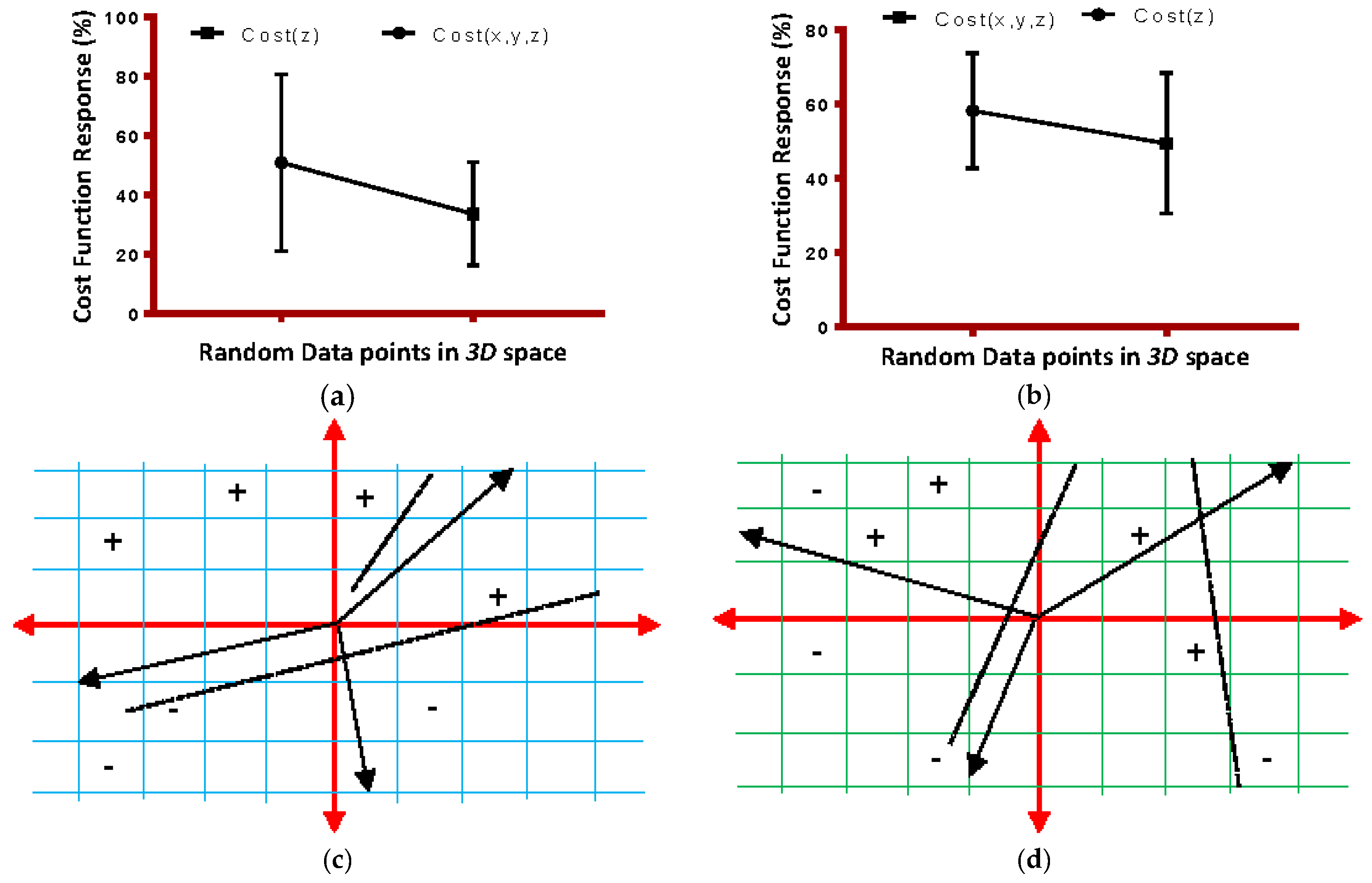Figure 5 shows the cost function variation in LT object for each coordinate.

PROCEDURE 2Scorebest ← Import all attributes as ‘n’
       Costbest ← n
       For j ← 1 to Iterationmax Do
          Cost ← Generate random number between 0 and Costbest
          Score ← Randomly select item from Cost feature
          If LT.InConsistance (Scorebest, Training Set) ≤ ∅ Then
		    Scorebest ← Score
		    Costbest ← C
       Return (Scorebest)
		

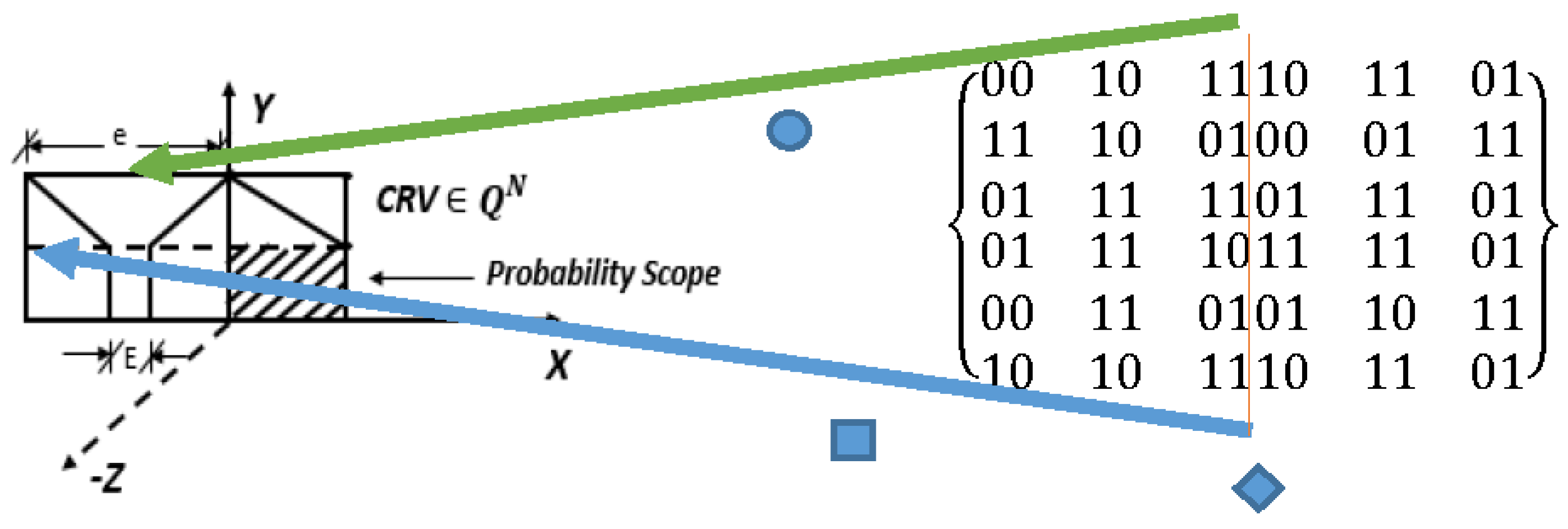
Definition 3.

Let lt.IrrF and lt.RedF be two functions to store the irrelevancy and redundancy score of each feature for a given dataset.

Let us define a Continuous Random Vector CRV ∈ Q^N, and Discrete Random Variable DRV ∈ H = {h₁,h₂,h₃,……..,h_n}. The density function of the random vector based on cumulative probability is P(CRV) = ${\sum }_{i=1}^N$P_H(h_i)p CRV|DRV, P_H(h_i) being a priori probability of class.

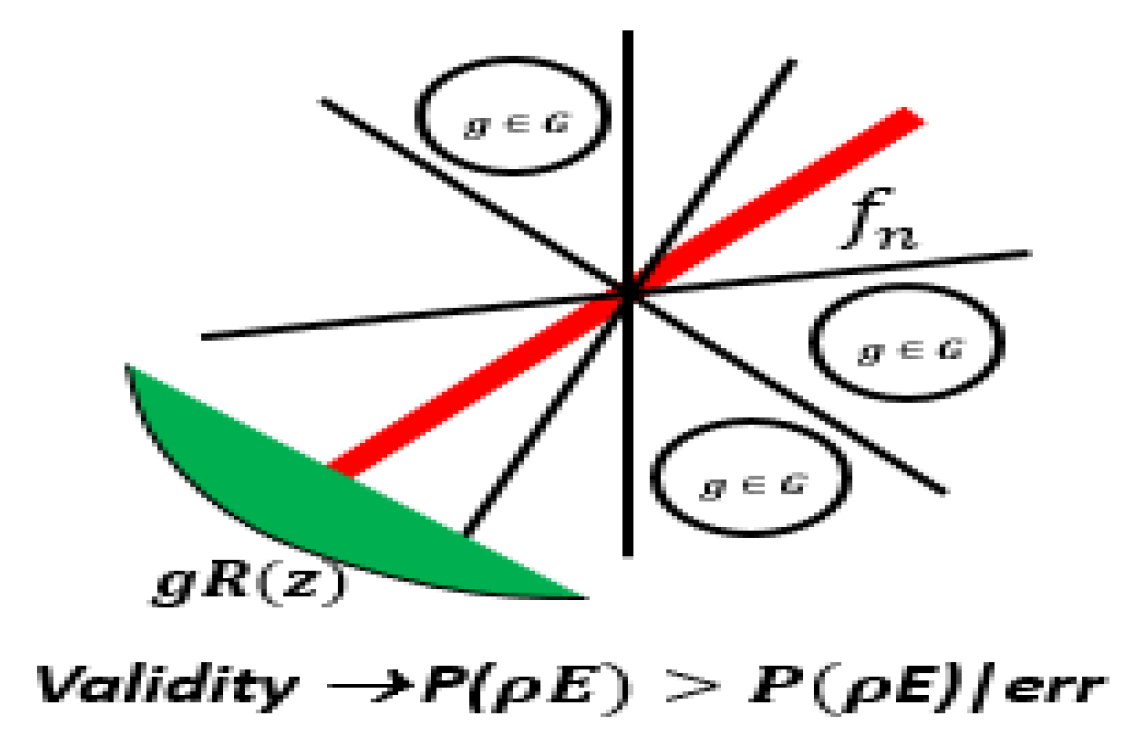
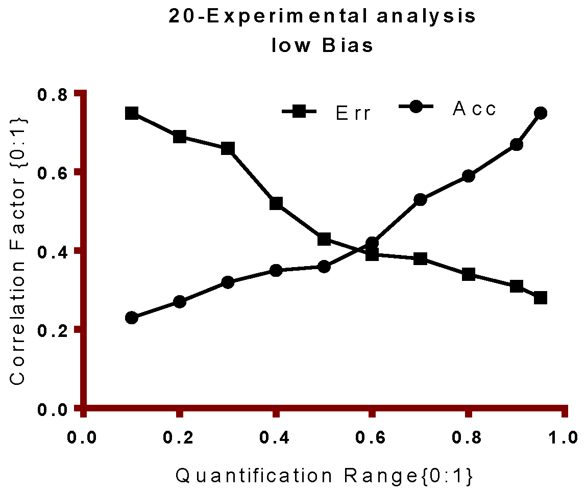
As we observe that the higher error limit (e) (err, green line, round symbol) and lower error limit (E), (Err, blue line, square symbol) bound the feature correlation in this process. Our aim is to spread the distribution in z-dimension for optimum fitting as features are added. The red line (diamond symbol) that separates the binary distribution of Redundant Feature (Red.F) and Irrelevant Features (Irr.F) based on error bounds. The green and red lines define the upper and lower limit of the error, in which all features correlate. Here, we build a mutual information (MI) function [14] so we can quantify the relevance of a feature upon other in the random set and this information is used to build the construct for Irr.F, since once our classifier learns, it will mature the Irr.F learning module as defined in the Algorithm 1.

$$MI(Irr.F(x,y,z)|f_i,f_{i+1}= {\displaystyle \sum }_{a=1}^N{\displaystyle \sum }_{b=1}^{N}p (f_i\left(a\right),f_{i+1}\left(b\right). log\left(\frac{f_i\left(a\right),f_{i+1}\left(b\right)}{p (f_i\left(a\right) . f_{i+1}\left(b\right)}\right)$$

(6)

We expect MI ← 0, for features to be statistically independent, so we build the construct in which the MI will be linearly related to the entropies of the features under test for Irr.F and Red.F, thus:

$$M.I\left(f_i, f_{i+1}\right)= \{\begin{array}{c}H\left(f_i\right)-H (f_i|f_{i+1})\\ H (f_{i+1}-H (f_{i+1}|f_i)\\ H\left(f_i\right)+ H\left(f_{i+1}\right)-H \left(f_i,f_{i+1}\right)\end{array}$$

(7)

We use the following construct to develop the relation of ‘Irr.F’ and ‘Red.F’ to show the irrelevancy factor and Redundant factor based on binary correlation and conflict mechanism as illustrated in above table.

$$Irr.F={\displaystyle \sum }_{i,j}^K\left\{\begin{array}{cc}{f}_{\mathit{ii}}& f_{\mathit{ij}}\\ f_{\mathit{ji}}& f_{\mathit{ji}}\end{array}\right\}Red.F=\{\begin{array}{l}\mathit{MI}(f_i; Irr.F)>0.5\hspace{1em}\hspace{1em}\mathit{Strong} \mathit{Relevant} \mathit{Feature}\\ \mathit{MI}(f_i; Irr.F)<0.5\hspace{1em}\hspace{1em}\mathit{Weak} \mathit{Relevant} \mathit{Feature}\\ \mathit{MI}(f_i; Irr.F)=0.5\hspace{1em}\hspace{1em}\mathit{Neutral} \mathit{Relevant} \mathit{Feature}\end{array}$$

(8)

Definition 4.

Globally in 3-D space, there exist three types of features types (variables), as predictor features:$PF = \left\{p{f}_1,p{f}_2,p{f}_3,\dots \dots ..p{f}_n\right\}$, and accepted features to be$AF = \left\{a{f}_1,a{f}_2,a{f}_3,\dots \dots ..,a{f}_n\right\}$and rejected features to be$RF=\left\{r{f}_1,r{f}_2,r{f}_3,\dots ..r{f}_n\right\}$, in which$\mathbb{G} \ge \left(g+1\right)$, global gain for all experimental occurrence of data samples. ‘$\mathbb{G}$’ being the global gain (GG). ‘$g$’ being the local gain (LG). Let PV be the predictive value. Accepted features are $a{f}_n\in PV$, strongly relevant to the sample data set $\Delta S$, if there exist at-least one x and z or y and z plane with score $\ge 0.8$, AND a single feature $f \in F$ is strongly relevant to the objective Function ‘ObF’ in distribution ‘d’ if there exist at-least a pair of example in data set {$\Delta S_1,\Delta S_2, \Delta S_3,\dots \dots ,\Delta S_n \in I\}$, such that d ($\Delta S_i) \ne 0$ and d ($\Delta S_{i+1}) \ne 0$. Let $\nabla \left(\phi ,\rho ,\omega \right)$ correspond to the acceptable maximum 3-axis function for possible optimum values of x, y, and z respectively.

We need to build an ideal classifier that learns from data during training and estimate the predictive accuracy, so it generalizes well on the testing data. We can use probabilistic theory of Bayesian [31] to develop a construct similar to direct table lookup. We assume a random variable to be ‘rV’ that will appear with many values in set of $\left\{r{V}_1, r{V}_2,r{V}_3,\dots , r{V}_n\right\} \mathrm{that}\mathrm{appear}\mathrm{as}\mathrm{a}\mathrm{class}.$ We will use prior probability $P \left(r{V}_i\right)$. Thus, we represent a class or set of classes as $r{V}_i,$ and the greatest $P \left(r{V}_i\right)$, for given pattern of evidence (pE) that classifier learns on $P (r{V}_i | pE) > P (r{V}_j| pE)$valid for all $i \ne j$.

Because we know that

$$P (r{V}_i | pE) = \frac{P (pE | r{V}_i) P \left(r{V}_i\right) }{ \left(P\left(pE\right)\right)}$$

(9)

Therefore, we can write the conditional equation where P (pE) is considered with regard to probability of (pE) is $P (pE | r{V}_i)P \left(r{V}_i\right) > P (pE | r{V}_j)P \left(r{V}_j\right)$valid for all $i \ne j$. Finally, we can write the probability of the error for the above given pattern, as P (pE)|error, assuming the cost function for all correct classification is 0, and for all incorrect is 1, then as stated earlier, the Bayesian classification will put the instance in the class labelling the highest posterior probability as $P \left(pE\right) = {\displaystyle \sum }_{i=1}^{k}P (r{V}_i) P (pE|r{V}_i)$. Therefore, the construct can thus be determined as $P \left(pE\right)|error = Error [1-max\{P \left(r{V}_1\right) | pE,\mathrm{\dots \dots },P (r{V}_k|pE)\}]$. Let us construct the matrix function of all features, accepted and rejected features, based on GG and LG, as

$$\mathbb{G} \left(x,y,z\right) = \frac{1}{N} {\displaystyle \sum }_{i=1}^n\{\left(g_i\right)\times MH\}$$

(10)

$$MH= \left\{\begin{array}{ccc}p{f}_{x1y1}& \dots & p{f}_{x1yn}\\ ⋮& \ddots & ⋮\\ p{f}_{xny1}& \dots & p{f}_{xnyn}\end{array}\right\} =\left\{\begin{array}{cccc}a{f}_{11}& a{f}_{12}& \dots & a{f}_{1n}\\ a{f}_{n1}& a{f}_{n2}& \dots & a{f}_{nm}\end{array}\right\}\times \left\{\begin{array}{cc}r{f}_{11}& r{f}_{1n}\\ r{f}_{21}& r{f}_{2n}\\ r{f}_{2n}& r{f}_{mn}\end{array}\right\} \pm \nabla \left(\phi ,\rho ,\omega \right)$$

(11)

Table 1. Typical observations of the functions.

$\mathbf{F}\mathbf{u}\mathbf{n}\mathbf{c}\mathbf{t}\mathbf{i}\mathbf{o}\mathbf{n}$	Min	Mid	Max
$\nabla \left(\phi ,\rho ,\omega \right)$	(0.21, 0.71, 0.44)	(0.43, 55, 49)	(0.81, 0.76, 58)
g (x, y, z)	(0.34, 0.51, −0.11)	(0.55, 0.51, 0.68)	(0.67, 71, 89)
$\mathbb{G} \left(x,y,z\right)$	(0.44, 0.55, 0.45)	(0.49, 0.59, 0.58)	(0.52, 0.63, 0.94)

shows the various ranges for Minimum, Maximum and Middle points of the all three functions as discussed earlier.

Using Naïve Bayes multicategory equality as:

$$P_{1,2,3,\dots ,N} \left[{\displaystyle \sum }_j{x}_j\right]+\left[{\displaystyle \sum }_j{y}_j\right]+\left[{\displaystyle \sum }_j{z}_j\right]= {\displaystyle \sum }_{k}Var\left(x,y,z\right)\left[z^{*}{}^i\right]$$

(12)

where $z^{*}\left(n\right)≔ \underset{z}{\mathrm{argmax}}P\left(z\right){\displaystyle \prod }_{k=1}^{n}p\left(\left[z\right]\right).z_k$, and Fisher score algorithm [3] can be used in FS to measure the relevance of each feature based on Laplacian score, such that $B\left(i,j\right)= \{\begin{array}{c}\frac{1}{N_l} if u_i= u_i=1\\ 0 otherwise,\end{array}$.

$N_l$ shows the no. of data samples in test class shown subscript ‘l’. Generally, we know that based on specific affinity matrix, $FISHE{R}_{score}\left(f_i\right)=1- \frac{1}{LAPCLACIA{N}_{score}\left(f_i\right)}$.

To group the features based on relevancy score, we must ensure that each group member of the features exhibit low variance, medium stability and their score is based on optimum-fitness, thus each member follows $k (k\in K, where K \le f \left(0:1\right)$. This also ensure that we address the high dimensionality issue, as when feature appears in high dimension, they tend to change their value for training mode, thus, we determine the information gain using entropy function as:

$$Entropy \left(F_n\right) = {\displaystyle \sum }_{t=1}^{V1}-p_t log p_t$$

(13)

V₁ indicates the number of various value of the target features in set of F. and $p_t$ is the probability of the type of value of t in a complete subset of the feature tested. Similarly, we can calculate the entropy for each feature in x, y, z dimension as:

$$Entropy \left(F_{n\in x,y,z}\right) = {\displaystyle \sum }_{t\in T \left(x,y,z\right)}\frac{\left| F_{ \left(t:x,y,z\right)}\right|}{\left|F_t\right|}Entropy \left(F_n\right)$$

(14)

Consequently, gain function in probability of entropy in 3D is determined as:

$$Gain \left(I, F_{ \left(t:x,y,z\right)}\right) = Entropy \left(F_n\right) - Entropy \left(F_{n\in x,y,z}\right)$$

(15)

We develop a ratio of gain for each feature in z-dimension as this ensure the maximum fitness of the feature set for the given predictive modeling in the given dataset for which ML algorithm needs to be trained. Thus, gR indicates the ratio between:

$$gR \left(z\right) = \frac{Gain \left(I, F_{ \left(t:x,y,z\right)}\right) }{\mathbb{G} \left(x,y,z\right)} |P \left(pE\right) > P \left(pE\right)|error$$

(16)

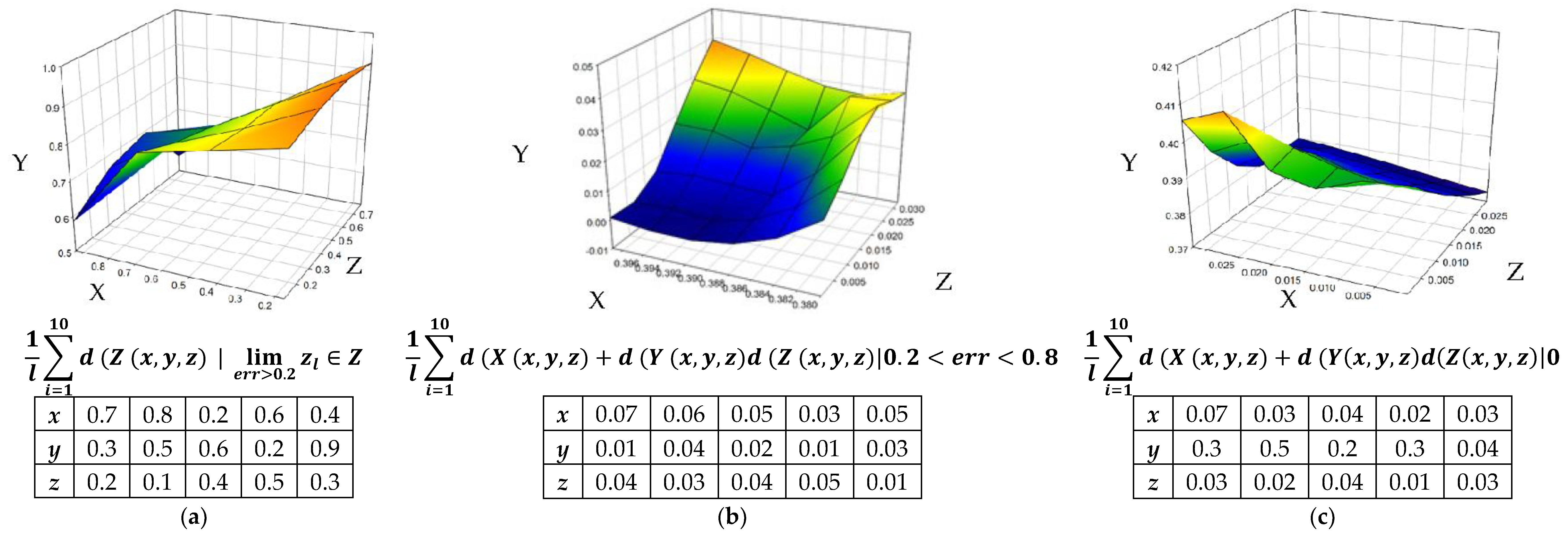
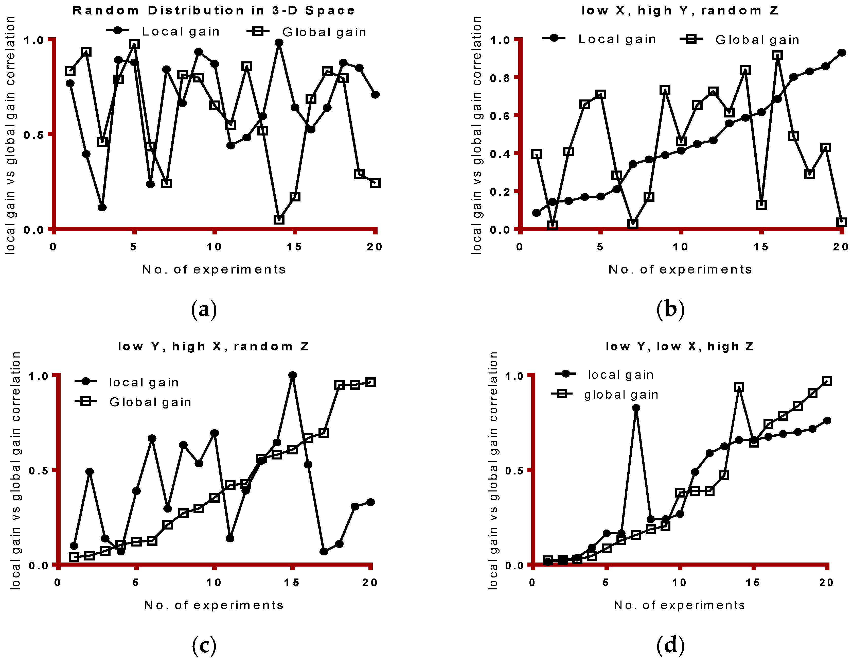
Figure 7 shows the displacement of the local gain and global gain functions based on probability distributions. As discussed earlier, LG and GG functions are developed to regulate the accuracy and thus validity of the classifier is measured initially based on accuracy metric.

Table 2. Typical observations.

	g (max)	G (min)	G (max)	g (min)
P (err)	0.25	0.45	0.31	0.56
P (Err)	0.32	0.41	0.49	0.59

shows the probability of local and global error limits based on probability function (Figure 7) in terms of local (g) and global gain function (G).

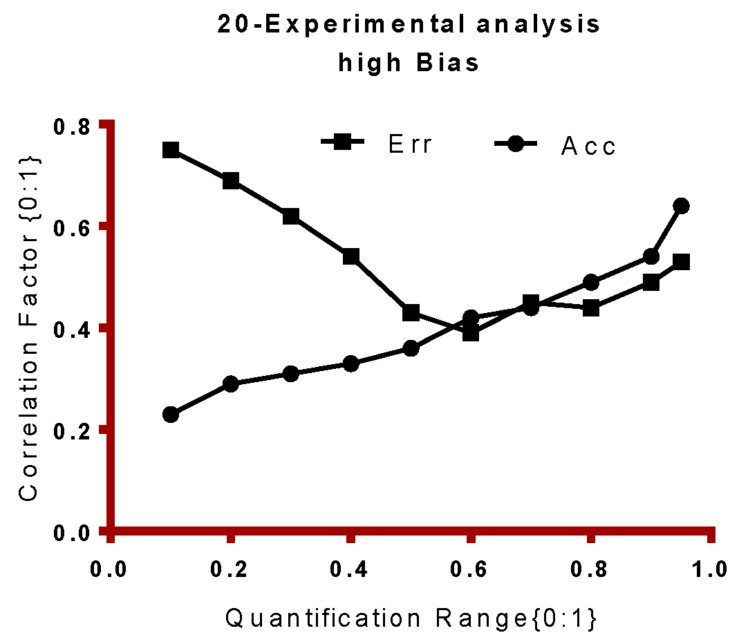
RULE 2If (g (err) < 0.2) Then
        Flag ‘O.F’
        Elseif (g (err) > 0.8) Flag ‘U.F’
		

If we assume the fact of $\{\Delta S_1,\Delta S_2, \Delta S_3,\dots \dots ,\Delta S_n \in I\}$, such that d ($\Delta S_i) \ne 0$ and d ($\Delta S_{i+1}) \ne 0$, where ‘I’ is the global input of testing data. We also confirm the relevance of the feature in the set using objective Function construct in distribution ‘d’, thus:

$$ObF \left(d, I\right) =\frac{log \left(Gain \left(I, F_{ \left(t:x,y,z\right)}\right)\right)}{ \left(err\left[max:1\left], err\right[min:0\right]\right)} \left| d \left(\Delta S_i\right) \ne 0 \right| for every F_i in group$$

(17)

Then, Using Equations (14)–(17), we can finally get

$$F.Eng\left(x,y,z\right)= \frac{1}{ \left(k\times M\right)} {\displaystyle \sum }_{t=1}^K{\displaystyle \prod }_{t=k}^{M}ObF \left(d, I\right) \times M{H}_t)$$

(18)

$$F.Grp\left(x,y,z\right)= F.Eng\left(x,0,0\right)+ F.Eng\left(0,y,0\right)- F.Eng\left(0,0,z\right)$$

(19)

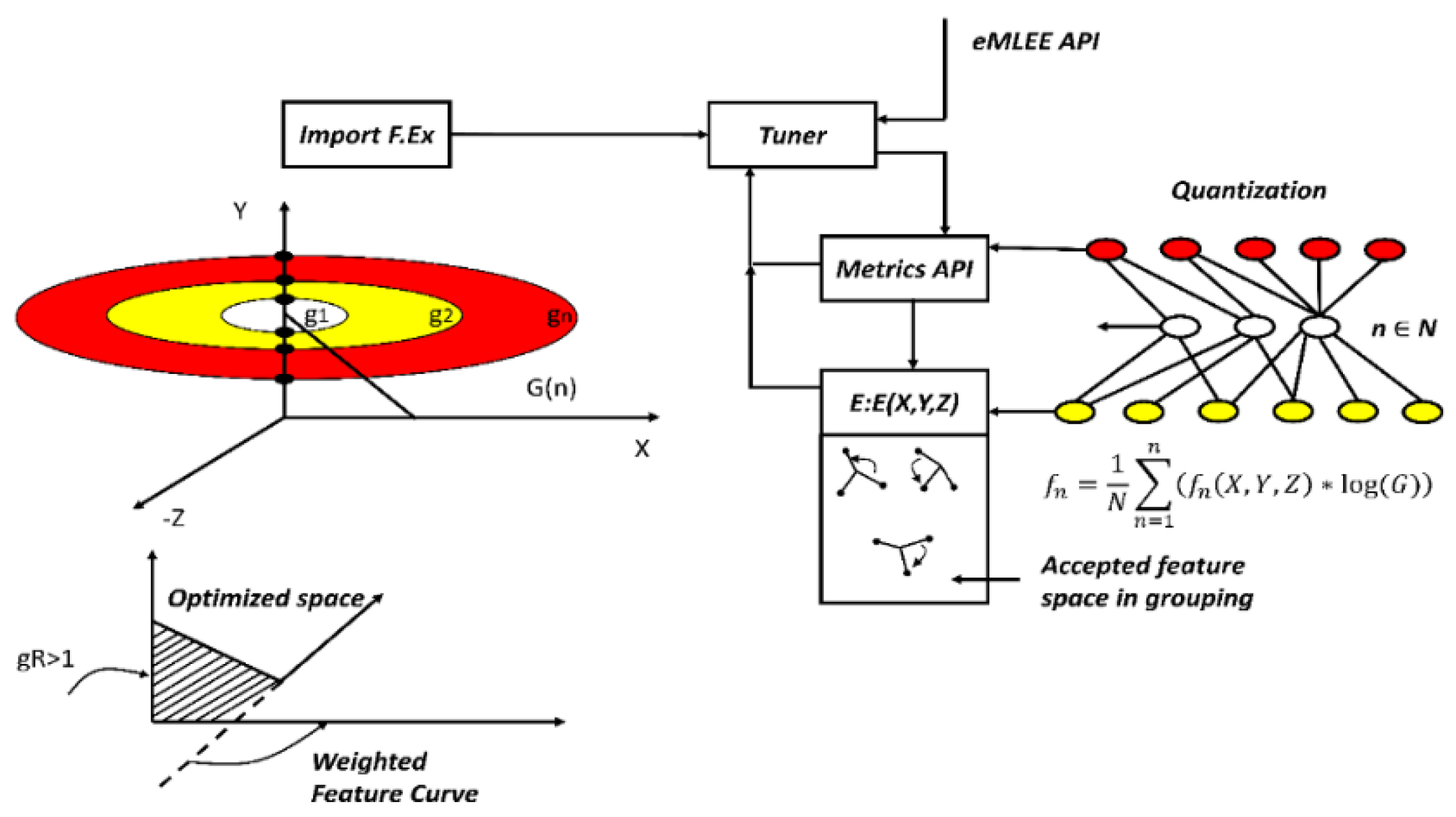
Figure 8 Illustration of Feature Engineering and Feature Group as constructed in the mathematical model and governed by the Algorithms 1 and 2, defined later. Metrics API is available from eMLEE package. The white, yellow, and red orbital shapes indicate the local gain progression through 3D space. The little 3D shapes (x, y, and z) in the accepted feature space in grouping indicates several (theoretically unlimited) instances of the optimized values as the quantization progresses.

Definition 5.

Feature selection is governed by satisfying the scoring function (score) in 3D space (x: Over-Fitness, y: Under-Fitness, z: Optimum-Fitness) for which evaluation criterion needs to be maximized, such that$Evaluation Criterion: f^{\prime }$. There exist a weighted,$W(\varnothing )\left\{\nabla \left(\phi ,\rho ,\omega \right), 1\right\}$function that quantifies the score for each feature, based on response from eMLEE engine with function$eMLE{E}_{return}$, such that each feature in$\left\{f_1, f_2, f_3,\dots \dots .., f_n,\right\}$, has associated score for$\left(\phi :x,y,z,\rho :x,y,z,\omega :x,y,z\right)$.

Two or more features may have the same predictive value and will be considered redundant. The non-linear relationship exists between two or more features (variables) that affects the stability and linearity of the learning process. If the incremental accuracy is improved, then non-linearity of a variable is ignored. As the number of the features are added or removed in the given set, the OF, UF, and B changes. Thus, we need to quantify their convergence, relevance, and covariance distribution across the space in 3D. We implement weighted function for each metric using LVQ technique [1], in which, we measure each metric over several experimental runs for enhanced feature set, as reported back from the function explained in Theorems 1 and 2, such that we optimize the z-dimension for optimum fitness and reduce x and y dimension for over-fitness and under-fitness. Let us define:

$$W(\varnothing )= \frac{1}{{{\displaystyle \int }}_{S_t}p\left(x\right)dx} {\displaystyle \sum }_{\gamma =1}^{\sigma }{N}_{\gamma }^T . N_{\gamma } \underset{S_{\gamma }}{{\displaystyle \int }}p\left(x\right)dx$$

(20)

where the piecewise effective decision border is $S_t= {\displaystyle \sum }_{\gamma =1}^{\sigma }{S}_{\gamma }$, In addition, the unit normal vector, ($N_{\gamma }$) for border $S_{\gamma }, \gamma =1, 2, 3, 4,\dots \dots .\sigma$ is valid for all cases in space. Let us define the probability distribution of data on $S_{\gamma } : {\mathbb{Q}}_{\gamma }= \underset{S_{\gamma }}{{\displaystyle \int }}p\left(x\right)dx.$ Here, we can use the Parzen method [32], to restore the nonparametric density estimation method, to estimate the ${\mathbb{Q}}_{\gamma }$.

$$\widehat{{\mathbb{Q}}_{\gamma } }(\Delta )= {\displaystyle \sum }_{j=1}^K\delta (d (x_i, S_{\gamma }) \le \frac{\Delta }{2}$$

(21)

where $d \left(x_i, S_{\gamma }\right)$ shows the Euclidean distance function. Figure 9 shows the Euclidean distance function based on binary weights for $W(\varnothing )$ function.

Table 3. Average Observations.

Function	Min	Max
$W(\varnothing )$	28.31%	78.34%
${\mathbb{Q}}_{\gamma }$	+0.2834	−0.1893

lists the quick comparison of the values of two functions as developed to observe the minimum and maximum bounds.

We used the Las Vegas Algorithm approach that helps to get correct solution at the end. We used it to validate the correctness of our gain function. This algorithm guarantees correct outcome if the solution is returned or created. It uses the probability approximate functions to implement runnable time-based instances. For our feature selection problem, we will have a set of features that will guarantee the optimum minimum set of features for acceptable classification accuracy. We use linear regression to compute the value of features to detect the non-linearity relationship between features, we thus implement a function, $Func\left(U\left(t\right)\right)=a+b\ast t$. Where a, and b are two test features and values can be determined by using linear regression techniques, so $b= \frac{{{\displaystyle \sum }}_{t=1}^T\left(t -\overline{ t}\right) (U\left(t\right) -\overline{ u)} }{{{\displaystyle \sum }}_{t=1}^T {\left(t - \overline{t}\right)}^2}$. Where, $a= \overline{u}-b\ast \overline{t}$, $\overline{u}= \frac{1}{T} {\displaystyle \sum }_{t=1}^{T}U \left(t\right)$, $\overline{t}= \frac{1}{T} {\displaystyle \sum }_{t=1}^{T}t$. These equations also minimize the squared error. To compute weighted function, we use feature ranking technique [12]. In this method, we will score each feature, based on quality measure such as information gain. Eventually, the large feature set will be reduced to a small feature set that is usable. The Feature Selection can be enhanced in several ways such as pre-processing, calculating information gain, error estimation, redundant feature or terms removal, and determining outlier’s quantification, etc. The information gain can be determined as:

$$\begin{gathered} Gai{n}_I(w)= - {\displaystyle \sum }_{j=1}^{M}P(M_j ). \log P(M_j)+P(w){\displaystyle \sum }_{j=1}^{M}P (M_j | w).\log P(M_j |w) \\ +P (\overline{w}) {\displaystyle \sum }_{j=1}^{M}P(M_j |\overline{w}) . \log P (M_j|\overline{w}) \end{gathered}$$

(22)

‘M’ shows the number of classes and ‘P’ is the probability. ‘W’ is the term that it contains as a feature. $P \left(M_{j }\right|w)$ is the conditional probability. In practice, the gain is normalized using Entropy, such as

$$Norm.Gai{n}_I\left(w\right)=\frac{\left\{Gai{n}_I\left(w\right)\right\}}{\left\{-\frac{n\left(w\right)}{n}\log \frac{n \left(w\right)}{n}\right\}}$$

(23)

Here we apply conventional variance-mean techniques. We can assume, $\max \nabla {\displaystyle \sum }_{\mathrm{i}=1}^{\mathrm{n}}{\mathsf{\phi }}_{\mathrm{i}}{\mathsf{\rho }}_{\mathrm{i}}{\mathsf{\omega }}_{\mathrm{i}}-{\displaystyle \sum }_{\mathrm{i}=1}^{\mathrm{n}}\log {\mathsf{\phi }}_{\mathrm{i}}{\mathsf{\rho }}_{\mathrm{i}}{\mathsf{\omega }}_{\mathrm{i}}$. The algorithm will ensure that ‘EC$\left\{\mathrm{F}.\mathrm{Sco}\left(\mathrm{x},\mathrm{y},\mathrm{z}\right),\mathrm{F}.\mathrm{Opt}\left(\mathrm{x},\mathrm{y},\mathrm{z}\right)\ge 0.5\right\}$’ stays in optimum bounds. Linear combination of Shannon information terms [7] and conditional mutual information maximization (CMIM) [3] for ${\mathrm{U}}_{\mathrm{MAX}}\left({\mathrm{Z}}_{\mathrm{k}}\right)=\underset{{\mathrm{Z}}_{\mathrm{k}}\in \Delta \mathrm{s}}{\max }\left[{\mathrm{Inf}(\mathrm{Z}}_{\mathrm{k}}:\mathrm{X},\mathrm{Y}|{\left(\mathrm{XY}\right)}_{\mathrm{k}}\right)]$ builds the functions as

$$Score\left(X|Y\right)= {\displaystyle \sum }_{y_k\in Y}G\left(y_k\right). {\displaystyle \sum }_{x_{k\prime }\in X}G \left(x_{k\prime }\right) \times \log \left(g\left(z\right)\right)$$

(24)

$$J_{MIN}{\left(Z\right)}^d= - \beta ({\displaystyle \prod }_{k,k\prime }^{K \left(0\right)}S{\left(X:Y\right)}_k+ \gamma ({\displaystyle \prod }_{k,k\prime }^{K \left(0\right)}S{\left(Y:X\right)}_{k\prime }$$

(25)

By using Equations (23)–(27), we get

$$F.Sco\left(x,y,z\right)= Score\left(X|Y\right)+ {\displaystyle \sum }_{i=1}^{n}W{(\varnothing )}_i-{{\displaystyle \sum }}_{j=1}^{n}Gai{n}_j\left(w\right)$$

(26)

$$F.Opt\left(x,y,z\right)= J_{MIN}{\left(Z\right)}^d.{\displaystyle \prod }_{F.Soc\left(x,y,z\right)}^N\left\{\frac{F.Soc\left(x,y,z\right)}{1+ТNorm.Gai{n}_I\left(w\right)}\right\}-{\displaystyle \sum }_{j=1}^n\Delta Err \left(j\right)$$

(27)

3.2. eFES Algorithms

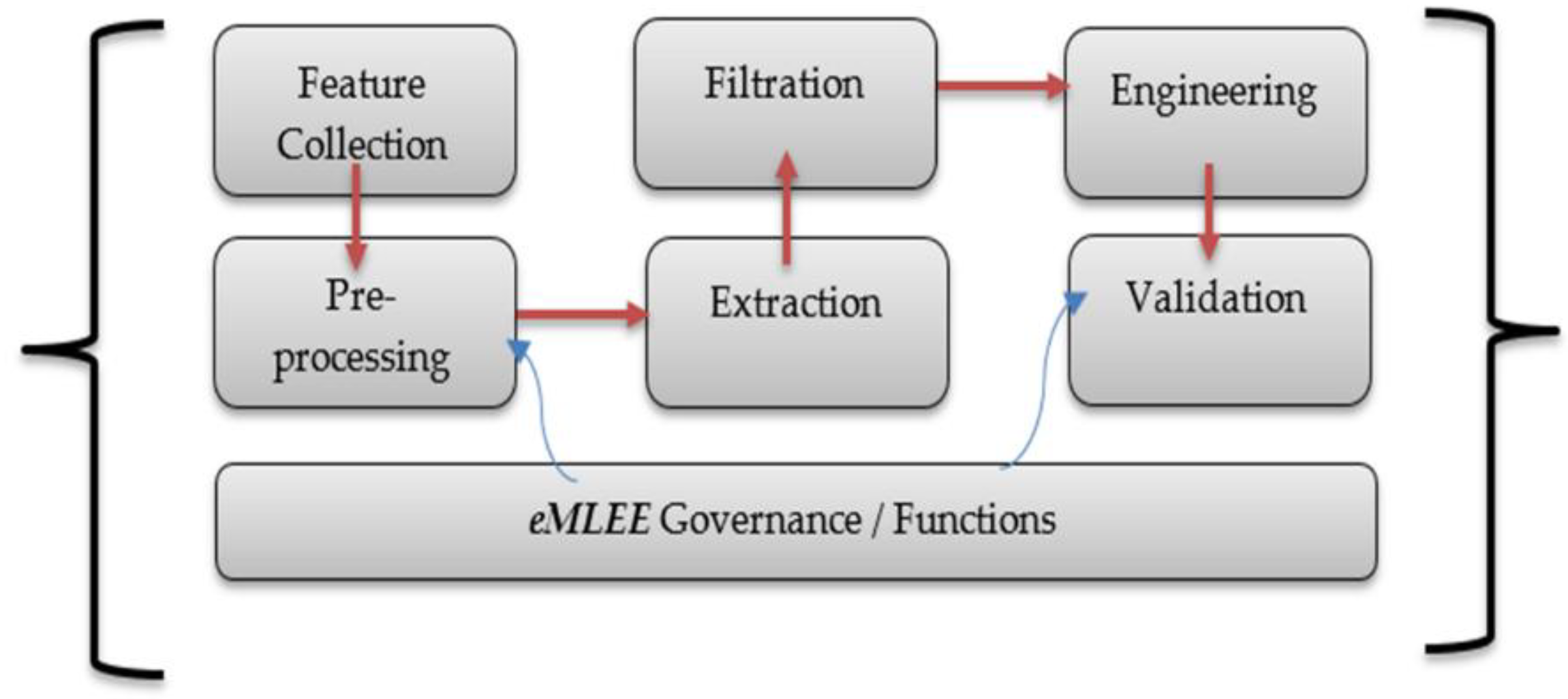
The following algorithms aim: (i) to compute functions as raw feature extraction, related features identification, redundancy, and irrelevancy to prepare the layer for feature pre-processing; (ii) to compute and quantify the selection and grouping factor for the acceptance as model incorporates them; and (iii) to compute the optimization function of the model, based on weights and scoring functions. objeMLEE is the API call for accessing public functions

Following are the pre-requisites for the algorithms.

Initialization: Set the algorithm libraries, create subset of the dataset for random testing and then correlating (overlapping) tests.

Create: LTObject for ${\mathrm{eFES}}^{⊞}$

Create: ObjeMLEE (h)/*create an object reference of eMLEE API */

Set: ObjeMLEE.PublicFunctions (h.eABT,h.eFES,h.eWPM,h.eCVS)/* Handles for all four constructs*/

Global Input: $A_n=\left\{A_1,A_2,A_3,\dots \dots ..,A_n\right\}$, $F_n=\left\{F_1,F_2,F_3,\dots \dots ..,F_n,\right\},DataSet\left(signal,noise\right)$

Dataset Selection: These algorithms require the dataset to be formatted and labelled with supervised learning in mind. These algorithms have been tested for miscellaneous datasets selected from different domains as listed in the appendix. Some preliminary clean-up may be needed depending upon the sources and raw format of the data. For our model building, we developed a Microsoft SQL Server-based data warehouse. However raw data files such as TXT and CSV are valid input files.

Overall Goal (Big Picture): The foremost goal of these two algorithms is to govern the mathematical model built-in eFES unit. These algorithms are essential to work in a chronological mode, as the output of Algorithm 1 is required for Algorithm 2. The core idea that algorithms utilize is to quantify each feature either in original, revealed or an aggregated state. Based on such scoring, which is very dynamic and parallelized while classifier learning is being governed by these algorithms, the feature is removed, added, or put on the waiting list, for the second round of screening. This is the beauty of it. For example, Feature-X may be scored low in the first round and because Feature-Y is now added, that impacts the scoring of the Feature-X, and thus Feature-X is upgraded by scoring function and included accordingly. Finally, algorithms accomplish the optimum grouping of the features from the dataset. This scheme maximizes the relevance, reduces the redundancy, improves the fitness, accuracy, and generalization of the model for improved predictive modeling in any datasets.

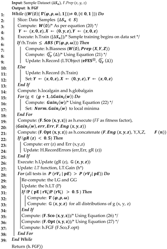
Algorithm 1 aims to compute the low-level function as F.Prep (x, y, z), based on final Equations (26) and (27) as developed in the model earlier. It uses the conditions of Irrelevant feature and Redundant feature functions and run the logic if the values are below 50% as a check criterion. This algorithm splits the training data based on popular approach as cross validation. However, it must be noted in line 6, that we use our model API for improving the value of k in the process, that we call enhanced cross validation. LT object regulates it and optimizes the value of k based on the classifier performance in the real time. It then follows the error rule (80%, 20%) and keeps track of each corresponding feature, as they are added or removed. Finally, it gets to the start using the gain function in 3D space for each fitting factor since our model is based on 3D scoring of each feature in the space where point is moved in x, y, and z values in space (logical tracking during classifier learning).

Algorithm 2 aims to use the output of algorithm 1 in conjunction with computing many other crucial functions to compute a final function of feature grouping function (FGF). It uses the weighted function to analyze each participating feature including the ones that were rejected. It also utilizes the LT object and its internal functions using the API. This algorithm slices the data into various non-overlapping segments. It uses one segment at a time, then randomly mixed them for more slices to improve the classifier generalization ability during the training phase. It uses ${\mathrm{eFES}}^{⊞}$ as a LT object from the library of eMLEE and records the coordinates for each feature. This way, entry is made in LT class, corresponding to the gain function as shown in lines 6 to 19. From line 29 to 35, it also uses probability distribution function, as explained earlier. It computes two crucial functions of $\nabla \left(\phi ,\rho ,\omega \right)$ and $\mathbb{G} \left(x,y,z\right)$. For this global gain (GG) function, each distribution of local gain g (x, y, z) must be considered as features come in for each test. All the low probability-based readings are discarded for active computation but kept in waiting list in the LT object for the second run. This way, algorithm does justice to each feature and give it a second chance before finally discarding it. The rest of the features that qualify in first or second run, are then added to the FGF.

Example 1.

In one of the experiments (such as Figure 13) on dataset with features including ‘RELIGION’, we discovered something very interesting and intuitive. The data was based on survey from students, as listed in the appendix. We then formatted some of the sets from different regions and ran our Good Fit Student (GFS) and Good Fit job Candidate (GFjC) algorithms (as we briefly discuss in future works). GFS and GFjC are based on eMLEE model and utilize eFES. We noticed as a pleasant surprise that in some cases, it rejected the RELIGION feature for GFS prediction and this made sense as normally religion will not influence success in the studies of the student, but then we discovered that it gave some acceptable scoring to the same feature, because it was coming from a different GEOGRAPHICAL region of the world. It made sense as well, because religion’s influence on the individual may be diverse depending on his or her background. We noticed that it successfully correlated with Correlation Factor (CF) > 0.83 on other features in the set and considered the associated feature to be given high score due to being appeared with the other features of the collateral importance (i.e., Geographical information). CF is one of the crucial factors in GFS and GFjC algorithms. GFS and GFjC are out of the scope of this paper.

Algorithm 1. Feature Preparation Function—F.Prep (x, y, z)

Another example was encountered where this feature played significant role in the job industry where a candidate’s progress can be impacted based on their religious background. Another example is of GENDER feature/attribute that we discuss in Section 6.1. This also explains our motivation towards creating FGF (Algorithm 2).

FGF function determines the right number and type of the features from a given data set during classifier learning and reports accordingly if satisfactory accuracy and generalization have not been reached. eFES unit, as explained in the model earlier, uses 3D array to store the scoring via LT object in the inner layer of the model. Therefore, eFES algorithms can tell the model if more features are needed to finally train the classifier for acceptable prediction in the real-world test.

Some other examples are data from healthcare, where a health condition (a feature) may become of high relevance if a certain disease is being predicted. For example, to predict the likelihood of cancer in a patient, DIABETES can have higher predictive score, because an imbalanced sugar can feed the cancerous cells. During learning, the classifier function starts identification of the features and then start adding or removing them based on effectiveness of the cost and time. Compared to other approaches where such proactive quantification is not done the eFES scheme dominates.

Algorithm 2. Feature Grouping Function (FGF)

Figure 10 simulations demonstrate the global gain and local gain functions coherences with respect to Loss and Cost functions. Figure 10a shows that gain function is unstable when eFES randomly created the feature set. Figure 10b shows that gain functions stabilize when eFES uses weighted function, as derived in the model.

3.3. eFES Framework

Figure 11 illustrates the internal functions of the proposed module on a granular level. eMLEE API refers to the available functions that eMLEE model provides to each module such as eFES. Each grey box is a function. The diamond shapes represent a decision-making point in the flow.

4. Results and Discussions

This section provides simulated results in 3D and 2D view to provide in-depth analysis of the outcome of the proposed model for various functions and metrics. Significant samples of the entire experimental results are provided at the latest state of this eFES model development stage. These simulations elaborate on processing features to observe the optimum fitness (i.e., z dimension). 3D visuals are selected for better analysis of how the curve moves in space when the learner is optimized in the dimensions. The equation below drives the experimental run for monitoring the z-dimension in correspondence to each of x, y, and z. It should be noted that the results shown are a snapshot of 100+ experimental runs for several data samples of the datasets. The equation shown for each indicates the sampling construct for the analysis being envisioned. Features were included in the experiments from the raw datasets. To improve the generalization of the model, various experiments were performed on standard numbers such as 5, 10, 15, 20 and 40. Clearly, less is more, as we stated earlier, but we leave it up to the model to finally group (FGF) the features that have the highest predictive value for learning and ensuring the maximum fitness and generalization. For each experiment, a miscellaneous dataset was used to improve the generalization ability of the model and underlying algorithms.

Figure 12 shows the 3D variance simulations of the functions. Figure 13 shows the comparison between features that were engineered (Enhanced Feature Engineering (EFE)) and that were not engineered (in blue). It is observed that EFE outperformed the FE. No FE indicates that the experiment took features set as per standard pick and ran the process. EFE indicates the enhanced feature engineering while incorporating mathematical constructs and algorithms, where features were added and removed based on metrics reading and eventually creating an optimum feature set, as engineered by eMLEE.

Figure 14a–d shows the tests on 20-experimental run. It should be noted that as the number of experiments were increased, the classifier learning was improved as per proposed model. The selection of 20 features were based on optimum number of the grouping function (FGF). Clearly, each dataset brings in different number of features. Out of these features, some features are irrelevant, redundant, and outliers. Some features are not known at the beginning of classifier learning. However, we standardized around number 20 for experimental purposes. However, it is up to the algorithm to tell the model how many features need to be qualified and then included in the learning process.

Figure 15a–e shows the test on (5, 10, 15, 20 and 50) features set. It compares the EFE and FE correlation for Fitness Factor (FF). FF is computed by the eFES algorithms explained earlier.

Figure 15 shows the set of experiments for observation of diverse set of features to study the model’s fitness factor. As it is observed that EFE keeps the linearity (stability) of the model. (e) was as special test of various metrics. “Engineered” refers to all the metrics of eFES model incorporated.

Figure 16 shows the three sets of 20-grouped feature sets. The goal of these experiments was to study the model ability to improve the accuracy for the features (Accepted, Rejected and Mixed) from the given data set.

Figure 17 shows the candlestick (commonly used for stock analysis) analysis for LE and GE bounds. It is observed that the model learned to stay in the bounds of 20% and 80% for LE and GE. Negative 50 range is shown to elaborate on potential of error swings (i.e., for invalid values). The green and purple sticks are for reference only.

Figure 18 and Figure 19 shows the observation of the bias of the model for 20-experimental analysis. Correlation Factor (CF) is computed by the eFES algorithms. Figure 18 shows the error and accuracy increases during higher end of quantification range as shown. Figure 19 on the other hand shows that the model has achieved the desired correlation of Err and Accuracy function.

Table 4. 10th experimental values for functions shown.

Internal Functions	1	2	3	4	5	6	7	8	9	10
$MI$	0.009	0.012	0.023	0.034	−0.931	0.563	0.611	0.678	0.712	0.731
$Irr.F\left(x,y,z\right)$	0.119	0.217	0.241	0.298	0.381	0.383	0.512	0.629	0.672	0.681
Red.F	0.191	0.200	−0.001	0.289	0.321	0.341	0.440	0.512	0.525	0.591
err	0.821	0.781	0.732	0.612	0.529	0.489	0.410	0.371	0.330	0.319
Err	0.901	0.900	0.871	0.844	0.731	−0.321	0.620	0.521	0.420	0.381
$F.Sco\left(x,y,z\right)$	0.390	0.421	0.498	0.534	0.634	0.721	0.770	0.812	0.856	0.891
$F.Opt\left(x,y,z\right)$	0.110	0.230	0.398	0.491	0.540	0.559	−0.210	0.639	0.776	0.791

shows the outcome of our 10-experimental analysis test, where we tuned the model to discover the maximum possible practical measures as shown. We used 500+ iterations on several different datasets to validate the model stability with real world data with the functions we built in our proposed model. Red values are found to be in error. Further work is needed to investigate it.

5. Comparative Analysis

This section provides a brief comparison of the latest techniques with the proposed model of eFES. The data sources are detailed in the Appendix.

Table 5. Data Sources (DS).

1	Breast Cancer Wisconsin Data Set
2	Car Evaluation
3	Iris species
4	Twitter User Gender Classification
5	College Scoreboard
6	Pima Indians Diabetes Database
7	Student Alcohol Consumption
8	Education Statistics
9	Storm Prediction center
10	Fatal Police Shootings
11	2015 Flight Delays and Cancellations
12	Credit Card Fraud Detection
13	Heart disease data set
14	Japan Census data
15	US Mass Shootings
16	Adult Census income
17	1.88 Million US Wildfires
18	S & P 500 stock Data
19	Zika Virus epidemic
20	Retail Data Analytics

shows the listing of the dataset used.

Table 6. Methods.

1	Information Gain	IG
2	Chi-squared	CS
3	Pearson Correlation	PC
4	Analysis of Variance	ANOVA
5	Weight of Evidence	WOE
6	Recursive Feature Elimination	RFE
7	Sequential Feature Selector	SFS
8	Univariant Selection	US
9	Principal Component Analysis	PCA
10	Random Forest	RF
11	Least Absolute Shrinkage and Selection Operator	LASSO
12	RIDGE Regression	RR
13	Elastic Net	EN
14	Gradient Boosted Machines	GBM
15	Linear discriminant analysis	LDA
	Multiple Discriminant Analysis	MDA
16	Joint Mutual Information	JMI
17	Non-negative matrix factorization	NNMF

lists the methods considered for the comparisons.

Table 7. Tables structures for 8 to 19.

Table Number	Measure	Number of the Datasets	Number of the Methods
8	Accuracy	1–10	1–10
9	Accuracy	11–20	11–17
10	Error	1–10	1–10
11	Error	11–20	11–17
12	Precision Score	1–10	1–10
13	Precision Score	11–20	11–17
14	C-Index	1–10	1–10
15	C-Index	11–20	11–17
16	AUC	1–10	1–10
17	AUC	11–20	11–17
18	Cohen’s Kappa	1–10	1–10
19	Cohen’s Kappa	11–20	11–17

lists the table structure of the division for results in

Table 8. Performance Evaluation (PE) = Accuracy, ideally higher values are desired.

DS	IG	CS	PC	ANOVA	WOE	RFE	SFS	US	PCA	RF	eFES	Winner
1	0.489	0.581	0.493	0.821	0.432	0.718	0.562	0.321	0.612	0.937	0.827	RF
2	0.391	0.501	0.452	0.732	0.479	0.700	0.590	0.476	0.842	0.842	0.863	eFES
3	0.429	0.543	0.572	0.683	0.481	0.681	0.623	0.419	0.693	0.534	0.633	PCA
4	0.444	0.492	0.365	0.601	0.538	0.710	0.512	0.478	0.793	0.792	0.825	eFES
5	0.492	0.572	0.392	0.621	0.593	0.661	0.652	0.563	0.824	0.312	0.881	eFES
6	0.482	0.563	0.592	0.910	0.582	0.633	0.692	0.673	0.847	0.118	0.792	ANOVA
7	0.523	0.557	0.673	0.666	0.523	0.502	0.619	0.693	0.734	0.492	0.700	PCA
8	0.542	0.599	0.962	0.732	0.710	0.682	0.638	0.478	0.892	0.692	0.983	eFES
9	0.423	0.630	0.921	0.802	0.504	0.623	0.742	0.732	0.872	0.631	0.902	PC
10	0.491	0.612	0.683	0.678	0.864	0.644	0.699	0.535	0.418	0.683	0.789	WOE

,

Table 9. Performance Evaluation (PE) = Accuracy.

DS	LASSO	RR	EN	GBM	LDA	MDA	JMI	NNMF	eFES	Winner
11	0.662	0.572	0.723	0.882	0.704	0.772	0.663	0.823	0.801	GBM
12	0.606	0.623	0.221	0.803	0.772	0.828	0.920	0.613	0.934	eFES
13	0.512	0.691	0.378	0.723	0.834	0.583	0.612	0.593	0.860	eFES
14	0.731	0.612	0.143	0.703	0.234	0.524	0.683	0.444	0.792	eFES
15	0.771	0.745	0.123	0.856	0.803	0.890	0.583	0.798	0.812	MDA
16	0.924	0.703	0.426	0.323	0.866	0.597	0.421	0.231	0.690	LASSO
17	0.832	0.791	0.484	0.428	0.792	0.890	0.792	0.166	0.942	eFES
18	0.883	0.723	0.923	0.573	0.723	0.748	0.842	0.772	0.793	EN
19	0.811	0.596	0.573	0.803	0.436	0.800	0.723	0.724	0.942	eFES
20	0.698	0.582	0.590	0.777	0.494	0.784	0.683	0.682	0.825	eFES

,

Table 10. Performance Evaluation (PE) = Error, ideally lower values are desired.

DS	IG	CS	PC	ANOVA	WOE	RFE	SFS	US	PCA	RF	eFES	Winner
1	0.254	0.443	0.623	0.234	0.112	0.213	0.487	0.126	0.111	0.173	0.223	PCA
2	0.231	0.193	0.423	0.278	0.321	0.183	0.215	0.193	0.213	0.213	0.201	RFE
3	0.593	0.318	0.283	0.318	0.294	0.143	0.368	0.216	0.172	0.229	0.045	eFES
4	0.443	0.244	0.342	0.087	0.221	0.193	0.125	0.259	0.193	0.281	0.112	ANOVA
5	0.183	0.289	0.124	0.213	0.084	0.426	0.258	0.442	0.145	0.342	0.014	eFES
6	0.392	0.173	0.192	0.282	0.103	0.083	0.159	0.044	0.039	0.293	0.023	eFES
7	0.361	0.111	0.009	0.045	0.115	0.063	0.193	0.310	0.135	0.183	0.216	PC
8	0.183	0.325	0.289	0.183	0.183	0.222	0.329	0.331	0.173	0.312	0.128	eFES
9	0.498	0.310	0.423	0.192	0.435	0.215	0.229	0.283	0.132	0.073	0.024	eFES
10	0.389	0.300	0.528	0.216	0.392	0.376	0.402	0.194	0.081	0.082	0.006	eFES

,

Table 11. Performance Evaluation (PE) = Error.

Δ∑	ΛAΣΣΟ	PP	EN	ΓBM	ΛΔA	MΔA	ϑMI	NNMΦ	εΦEΣ	Ωιννερ
11	0.092	0.175	0.134	0.097	0.281	0.145	0.113	0.130	0.073	εΦEΣ
12	0.125	0.179	0.111	0.173	0.173	0.100	0.193	0.193	0.034	εΦEΣ
13	0.214	0.231	0.190	0.239	0.151	0.182	0.231	0.210	0.111	εΦEΣ
14	0.163	0.200	0.138	0.166	0.088	0.163	0.009	0.003	0.183	NNMΦ
15	0.193	0.193	0.083	0.129	0.210	0.219	0.122	0.122	0.178	EN
16	0.236	0.437	0.238	0.321	0.134	0.110	0.177	0.191	0.088	εΦEΣ
17	0.173	0.432	0.110	0.146	0.443	0.325	0.212	0.253	0.134	EN
18	0.113	0.267	0.193	0.191	0.392	0.283	0.154	0.099	0.004	εΦEΣ
19	0.172	0.167	0.183	0.219	0.108	0.200	0.121	0.111	0.312	ΛΔA
20	0.283	0.045	0.128	0.183	0.214	0.204	0.231	0.131	0.021	εΦEΣ

,

Table 12. Performance Evaluation (PE) = Precision Score, ideally higher values are desired.

DS	IG	CS	PC	ANOVA	WOE	RFE	SFS	US	PCA	eFES	Winner
1	0.677	0.899	0.961	0.520	0.755	0.816	0.820	0.639	0.792	0.723	CS
2	0.936	0.755	0.553	0.600	0.522	0.690	0.776	0.764	0.841	0.802	IG
3	0.861	0.874	0.779	0.834	0.647	0.844	0.677	0.907	0.744	0.689	CS
4	0.545	0.603	0.882	0.850	0.725	0.637	0.887	0.554	0.754	0.956	eFES
5	0.767	0.584	0.894	0.861	0.761	0.915	0.753	0.513	0.909	0.932	eFES
6	0.753	0.557	0.664	0.707	0.706	0.732	0.622	0.714	0.804	0.762	PCA
7	0.814	0.585	0.865	0.667	0.790	0.620	0.781	0.773	0.933	0.903	PCA
8	0.546	0.706	0.852	0.902	0.619	0.710	0.732	0.738	0.638	0.967	eFES
9	0.859	0.760	0.610	0.627	0.617	0.673	0.591	0.803	0.575	0.992	eFES
10	0.698	0.710	0.702	0.674	0.821	0.691	0.503	0.781	0.746	0.710	US

,

Table 13. Performance Evaluation (PE) = Precision Score.

DS	RF	LASSO	RR	EN	GBM	LDA	MDA	JMI	NNMF	eFES	Winner
11	0.733	0.763	0.824	0.473	0.610	0.786	0.522	0.731	0.862	0.893	eFES
12	0.838	0.864	0.549	0.772	0.584	0.910	0.760	0.706	0.631	0.845	LDA
13	0.611	0.964	0.928	0.781	0.565	0.703	0.550	0.827	0.908	0.923	LASSO
14	0.905	0.923	0.754	0.807	0.643	0.670	0.605	0.531	0.650	0.982	eFES
15	0.640	0.601	0.820	0.950	0.512	0.948	0.827	0.786	0.662	0.734	EN
16	0.530	0.690	0.621	0.622	0.808	0.934	0.630	0.537	0.931	0.956	eFES
17	0.547	0.825	0.512	0.711	0.740	0.877	0.766	0.697	0.561	0.893	eFES
18	0.632	0.642	0.891	0.670	0.864	0.665	0.774	0.902	0.702	0.962	eFES
19	0.728	0.671	0.720	0.726	0.743	0.582	0.550	0.781	0.631	0.704	JMI
20	0.836	0.746	0.574	0.585	0.979	0.872	0.758	0.941	0.952	0.942	GBM

,

Table 14. Performance Evaluation (PE) = C-Index, ideally lower values are desired.

DS	IG	CS	PC	ANOVA	WOE	RFE	SFS	US	PCA	eFES	Winner
1	0.412	0.333	0.236	0.294	0.226	0.062	0.421	0.427	0.215	0.118	eFES
2	0.319	0.256	0.393	0.106	0.433	0.078	0.361	0.128	0.235	0.056	eFES
3	0.207	0.251	0.271	0.118	0.134	0.307	0.222	0.338	0.211	0.312	ANOVA
4	0.523	0.220	0.058	0.052	0.203	0.325	0.061	0.439	0.040	0.189	PCA
5	0.134	0.534	0.476	0.137	0.144	0.387	0.199	0.114	0.105	0.210	PCA
6	0.627	0.425	0.285	0.243	0.448	0.274	0.488	0.186	0.181	0.034	eFES
7	0.113	0.193	0.152	0.498	0.200	0.036	0.025	0.149	0.071	0.092	SFS
8	0.167	0.273	0.410	0.128	0.105	0.435	0.139	0.193	0.148	0.192	WOE
9	0.291	0.221	0.096	0.291	0.326	0.448	0.161	0.235	0.211	0.073	eFES
10	0.093	0.293	0.407	0.488	0.200	0.179	0.341	0.472	0.040	0.002	eFES

,

Table 15. Performance Evaluation (PE) = C-Index.

DS	RF	LASSO	RR	EN	GBM	LDA	MDA	JMI	NNMF	eFES	Winner
11	0.054	0.314	0.314	0.036	0.150	0.219	0.201	0.190	0.019	0.112	NNMF
12	0.268	0.217	0.293	0.252	0.552	0.209	0.318	0.394	0.219	0.243	LDA
13	0.542	0.325	0.320	0.327	0.346	0.245	0.249	0.322	0.403	0.296	LDA
14	0.282	0.141	0.251	0.132	0.136	0.360	0.217	0.224	0.232	0.106	eFES
15	0.043	0.060	0.210	0.021	0.093	0.264	0.091	0.247	0.136	0.129	RF
16	0.060	0.053	0.200	0.100	0.055	0.252	0.155	0.056	0.078	0.031	eFES
17	0.200	0.053	0.331	0.140	0.040	0.107	0.216	0.335	0.247	0.013	eFES
18	0.327	0.233	0.258	0.295	0.290	0.346	0.334	0.378	0.329	0.297	LASSO
19	0.094	0.196	0.312	0.309	0.066	0.216	0.128	0.164	0.258	0.032	eFES
20	0.073	0.263	0.204	0.064	0.053	0.206	0.010	0.239	0.047	0.024	MDA

,

Table 16. Performance Evaluation (PE) = AUC, ideally higher values are desired.

DS	IG	CS	PC	ANOVA	WOE	RFE	SFS	US	PCA	eFES	Winner
1	0.569	0.808	0.739	0.633	0.848	0.563	0.518	0.540	0.874	0.810	PCA
2	0.513	0.796	0.800	0.643	0.610	0.659	0.618	0.664	0.589	0.762	CS
3	0.784	0.636	0.781	0.589	0.499	0.585	0.539	0.858	0.717	0.96	eFES
4	0.592	0.834	0.498	0.788	0.789	0.713	0.911	0.830	0.645	0.976	eFES
5	0.655	0.698	0.805	0.504	0.880	0.574	0.638	0.885	0.742	0.699	WOE
6	0.590	0.741	0.791	0.825	0.654	0.826	0.698	0.679	0.962	0.892	PCA
7	0.802	0.626	0.680	0.510	0.896	0.745	0.646	0.735	0.974	0.740	PCA
8	0.805	0.560	0.550	0.826	0.609	0.812	0.659	0.704	0.814	0.894	eFES
9	0.642	0.802	0.769	0.891	0.504	0.482	0.629	0.830	0.734	0.836	ANOVA
10	0.872	0.898	0.858	0.785	0.921	0.573	0.831	0.754	0.868	0.971	eFES

,

Table 17. Performance Evaluation (PE) = AUC.

DS	RF	LASSO	RR	EN	GBM	LDA	MDA	JMI	NNMF	eFES	Winner
11	0.725	0.835	0.889	0.751	0.545	0.706	0.676	0.562	0.518	0.774	RR
12	0.889	0.819	0.532	0.555	0.890	0.751	0.946	0.688	0.778	0.903	MDA
13	0.568	0.835	0.520	0.525	0.502	0.764	0.605	0.651	0.487	0.952	eFES
14	0.780	0.728	0.606	0.870	0.792	0.545	0.553	0.855	0.990	0.962	NNMF
15	0.602	0.615	0.833	0.700	0.804	0.493	0.645	0.616	0.899	0.867	NNMF
16	0.736	0.649	0.589	0.665	0.848	0.847	0.905	0.621	0.897	0.952	eFES
17	0.541	0.711	0.777	0.511	0.868	0.884	0.691	0.904	0.665	0.962	eFES
18	0.796	0.525	0.768	0.762	0.755	0.513	0.759	0.910	0.599	0.852	eFES
19	0.873	0.481	0.606	0.639	0.558	0.575	0.783	0.842	0.675	0.820	RF
20	0.860	0.365	0.893	0.603	0.893	0.840	0.829	0.646	0.496	0.824	GBM

,

Table 18. Performance Evaluation (PE) = Cohen’s Kappa, ideally higher values are desired.

DS	IG	CS	PC	ANOVA	WOE	RFE	SFS	US	PCA	eFES	Winner
1	0.666	0.816	0.913	0.621	0.206	0.656	0.930	0.978	0.586	0.912	US
2	0.762	0.754	0.502	0.926	0.959	0.774	0.915	0.566	0.875	0.925	WOE
3	0.921	0.207	0.691	0.757	0.920	0.520	0.846	0.932	0.758	0.623	US
4	0.693	0.542	0.673	0.500	0.765	0.924	0.647	0.501	0.824	0.957	eFES
5	0.773	0.533	0.775	0.615	0.814	0.535	0.682	0.536	0.878	0.856	PCA
6	0.685	0.910	0.568	0.606	0.698	0.831	0.646	0.902	0.851	0.945	eFES
7	0.635	0.716	0.676	0.793	0.593	0.802	0.843	0.671	0.930	0.991	eFES
8	0.667	0.877	0.918	0.751	0.854	0.930	0.794	0.527	0.936	0.875	PCA
9	0.897	0.644	0.454	0.517	0.762	0.802	0.685	0.865	0.650	0.834	IG
10	0.599	0.824	0.803	0.802	0.827	0.875	0.933	0.851	0.724	0.925	eFES

and

Table 19. Performance Evaluation (PE) = Cohen’s Kappa.

DS	RF	LASSO	RR	EN	GBM	LDA	MDA	JMI	NNMF	eFES	Winner
11	0.892	0.929	0.819	0.874	0.537	0.662	0.833	0.581	0.857	0.983	eFES
12	0.954	0.660	0.944	0.489	0.582	0.869	0.753	0.786	0.771	0.973	eFES
13	0.576	0.952	0.686	0.588	0.744	0.712	0.658	0.927	0.671	0.910	LASSO
14	0.519	0.780	0.505	0.850	0.603	0.731	0.942	0.975	0.958	0.846	JMI
15	0.985	0.846	0.903	0.591	0.584	0.750	0.617	0.945	0.892	0.904	RF
16	0.786	0.804	0.605	0.673	0.814	0.635	0.909	0.573	0.732	0.973	eFES
17	0.827	0.567	0.814	0.772	0.867	0.890	0.670	0.771	0.763	0.734	LDA
18	0.751	0.733	0.820	0.813	0.760	0.637	0.871	0.739	0.867	0.923	eFES
19	0.698	0.645	0.636	0.801	0.727	0.886	0.969	0.954	0.781	0.845	MDA
20	0.583	0.646	0.795	0.930	0.953	0.523	0.681	0.565	0.524	0.578	EN

. The Python and R packages used are detailed in the tools sub-section of the Appendix. All the values are normalized to range between 0 and 1 for our functions’ standard outcome measures. It should be noted that the data shown in Table 8, Table 9, Table 10, Table 11, Table 12, Table 13, Table 14, Table 15, Table 16, Table 17, Table 18 and Table 19 are a subset of our total experimental analysis. The rest of the results are left out for our literature review and model comparison paper for future work/writings.

6. Final Remarks

6.1. Conclusions

This paper reports the latest progress of the proposed model for enhanced Feature Engineering and Selection (eFES) including mathematical constructs, framework, and the algorithms. eFES is a module of enhanced Machine Learning Engine Engineering (eMLEE) parent model. eFES is based on the following building blocks: (a) a features set is processed through standard methods and records the measured metrics; (b) features are weighted based on learning process where accepted features and rejected features are separated using 3D-based training through building Local Gain (LG) and Global Gain (GG) functions; (c) features are then scored and optimized so the ML process can evolve into deciding which features need to be accepted or rejected for improved generalization of the model; (d) finally features are evaluated, tested, and the model is completed with feature grouping function (FGF). This paper reports observation on several hundreds of experiments and then implements 10 experimental approaches to tune the model. The 10th experimental rule was adopted to narrow down (i.e., slice) the result extraction from several hundred runs. The LG and GG functions were built and optimized in 3D space. The included results show promising outcomes of the proposed scheme of the eFES model. It supports the use of feature sets to further optimize the learning process of ML models for supervised learning. Using the novel approach of Local Error and Global Error bounds of 20% to 80%, we could tune our model more realistically. If the errors were above 80% or below 20%, we flag it to be an invalid fit. This unique approach of engineering a model turns out to be very effective in our experiments and observations, as reported and discussed in this paper. This model though is based on parallel processing but using high-speed hardware or a Hadoop-based system will help further.

Features (i.e., attributes) in the datasets are often irrelevant and redundant and may have less predictive value. Therefore, we constructed these two functions. A) Irrelevant Irr.F (Equation (8)) and B) Red.F (Algorithm 1). The real-world data may have more features and based on this exact fact, we realized the gap to fill with our work. For ML model classifier learning, features play a crucial role when it comes to speed, performance, predictive accuracy, and reliability of the model. Too many features or too few features may overfit or underfit the model. Then the question becomes, what is the optimum (i.e., the right number) feature set that should be filtered for a ML process, that is where our work comes in. We wanted to have the model decides for itself as it continues to learn with more data. Certain features such as” Gender” or ”Sex” may have extreme predictive value (i.e., weight) for building predictive modeling for an academic data from a part of the world where gender bias is high. However, the same feature may not play a significant role when it is included in a set from a domain, where gender bias may not exist. Moreover, we also do not anticipate that based on our thoughts, but we let our model tell us which feature should be included or removed, thus we have two functions, Adder ($+\mathbb{F}\left(x,y,z\right)$) Equation (1) and Remover ($-\mathbb{F}\left(x,y,z\right)$) Equation (2). Number ”20” for features was selected to optimize around this number. Figure 15a–e shows the tests for 5, 10, 15 and 20 to observe the fitness factor. Table 7, Table 8, Table 9, Table 10, Table 11 and Table 12 in Section 5 show the promising state of eFES as compared to the existing techniques. It performed very well, generally. Parallel processing and 3D engineering of the features functions greatly improved the FO as we intended to investigate and improved with our work. Future work will further enhance the internals of it.

In some of the experimental tests, we came across some invalid outcomes, where we had to re-tune our model. Clearly, every model build-up process contains such issues where more work/investigation is always needed. We have found that such issues are not reflective of any huge inaccuracy in the results or instability of the model. Specially, in our diverse and stress testing, the errors and unexpected behavior and readings were very little as compared to stable and expected results. It should be watched closely with future enhancements and results, so it does not grow and become a real bug. This model is based on supervised learning algorithms.

6.2. Future Works

To further improve the current state of the eMLEE and its components (such as reported in this paper), we will be testing more data specifically from http://www.kaggle.com, www.data.gov, and www.mypersonality.org. We will be developing/testing more algorithms, especially in the domains of unsupervised learning for new insights into feature engineering and selection. Also, eFES needs further extensions towards exploring and engineering unknown features that are normally not encountered by the learning process but may have great predictive value. We are improving/developing a model known as the “Predicting Educational Relevance for an Efficient Classification of Talent (PERFECT)” Algorithm Engine (PAE). PAE is based on eMLEE and incorporates three algorithms known as Noise Removal and Structured Data Detection (NR-SDD), Good Fit Student (GFS), and Good Fit job Candidate (GFjC). We have published the preliminary results [33] and are working to apply the eFES (i.e., eMLEE) model in its latest form to study/explore/validate further enhancements.