End-to-End Neural Optical Music Recognition of Monophonic Scores

Abstract

Optical Music Recognition is a field of research that investigates how to computationally decode music notation from images. Despite the efforts made so far, there are hardly any complete solutions to the problem. In this work, we study the use of neural networks that work in an end-to-end manner. This is achieved by using a neural model that combines the capabilities of convolutional neural networks, which work on the input image, and recurrent neural networks, which deal with the sequential nature of the problem. Thanks to the use of the the so-called Connectionist Temporal Classification loss function, these models can be directly trained from input images accompanied by their corresponding transcripts into music symbol sequences. We also present the Printed Images of Music Staves (PrIMuS) dataset, containing more than 80,000 monodic single-staff real scores in common western notation, that is used to train and evaluate the neural approach. In our experiments, it is demonstrated that this formulation can be carried out successfully. Additionally, we study several considerations about the codification of the output musical sequences, the convergence and scalability of the neural models, as well as the ability of this approach to locate symbols in the input score.

1. Introduction

During the past few years, the availability of huge collections of digital scores has facilitated both the music professional practice and the amateur access to printed sources that were difficult to obtain in the past. Some examples of these collections are the IMSLP (http://imslp.org) website with currently 425,000 classical music scores, or many different sites offering Real Book jazz lead sheets. Furthermore, many efforts are being done by private and public libraries to publish their collections online (see http://drm.ccarh.org/). However, in addition to this instant availability, the advantages of having the digitized image of a work over its printed material are restricted to the ease to copy and distribute, and the lack of wear that digital media intrinsically offers over any physical resource. The great possibilities that current music-based applications can offer are restricted to scores symbolically encoded. Notation software such as Finale (https://www.finalemusic.com), Sibelius (https://www.avid.com/en/sibelius), MuseScore (https://musescore.org), or Dorico (https://www.steinberg.net/en/products/dorico), computer-assisted composition applications such as OpenMusic (http://repmus.ircam.fr/openmusic/), digital musicology systems such as Music21 (http://web.mit.edu/music21/), or Humdrum (http://www.humdrum.org/), or content-based search tools [1], cannot deal with pixels contained in digitized images but with computationally-encoded symbols such as notes, bar-lines or key signatures.

Furthermore, the scientific musicological domain would dramatically benefit from the availability of digitally encoded music in symbolic formats such as MEI [2] or MusicXML [3]. Just to name an example, many of the systems presented in the Computational Music Analysis book edited byMeredith [4] cannot be scaled to real-world scenarios due to the lack of big enough symbolic music datasets.

Many different initiatives have been proposed to manually fill this gap between digitized music images and digitally encoded music content such as OpenScore (https://openscore.cc), KernScores (http://kern.ccarh.org), or RISM [5]—encoding just small excerpts (incipits). However, the manual transcription of music scores does not represent a scalable process, given that its cost is prohibitive both in time and resources. Therefore, to face this scenario with guarantees, it is necessary to resort to assisted or automatic transcription systems. The so-called Optical Music Recognition (OMR) is defined as the research about teaching computers how to read musical notation [6], with the ultimate goal of exporting their content to a desired format.

Despite the great advantages of its development, OMR is far from being totally reliable as a black box, as current optical character recognition [7] or speech recognition [8] technologies do. Commercial software is constantly being improved by fixing specific problems from version to version. In the scientific community, there are hardly any complete approach for its solution [9,10]. Traditionally, this has been motivated because of the small sub-tasks in which the workflow can be divided. Simpler tasks such as staff-line removal, symbol localization and classification, or music notation assembly, have so far represented major obstacles [11]. Nonetheless, recent advances in machine learning, and specifically in Deep Learning (DL) [12], not only allow solving these tasks with some ease, but also to propose new schemes with which to face the whole process in a more elegant and compact way, avoiding heuristics that make systems limited to the kind of input they are designed for. In fact, this new sort of approaches has broken most of the glass-ceiling problems in text and speech recognition systems [13,14].

This work attempts to be a seed work that studies the suitability of applying DL systems to solve the OMR task holistically, i.e., in an end-to-end manner, without the need of dividing the problem into smaller stages. For this aim, two contributions are introduced. First, a thorough analysis of a DL model for OMR, and the design and construction of a big enough quality dataset on which training and evaluating the system. Note that the most difficult obstacle that researchers usually find when trying to apply DL algorithms is the lack of appropriate ground-truth data, which leads to a deadlock situation; that is, learning systems need big amounts of labeled data to train, and the fastest way of getting such amounts of labeled data is the use of trained systems. We therefore aim at unblocking such scenario in our proposal.

Considering this as a starting point, we restrict ourselves in this work to the consideration of monodic short scores taken from real music works in Common Western Modern Notation (CWMN). This allows to encode the expected output as a sequence of symbols that the model must predict. Then, one can use the so-called Connectionist Temporal Classification (CTC) loss function [15], with which the neural network can be trained in an end-to-end fashion. It means that it is not necessary to provide information about the composition or location of the symbols in the image, but only pairs of input scores and their corresponding transcripts into music symbol sequences.

As mentioned previously, a typical drawback when developing this research is the lack of data. Therefore, to facilitate the development of our work, we also propose an appropriate dataset to train and evaluate the neural model. Its construction is adapted for the task of studying DL techniques for monodic OMR, so two considerations must be taken into account. On the one hand, the output formats devised here do not aim at substituting any of the traditional music encodings [16]. On the other hand, although some previous efforts have been done to build datasets for this purpose [17,18], none of them fits the requirements of size and nature required for our study.

It must be kept in mind that our approach has been preliminarily evaluated on synthetic music scores [19], and so we want to further study here its potential. More precisely, the contributions of this work are listed as follows:

• Consideration of different formulations with respect to the output representation. We will see that the way of representing the symbol sequence is not trivial, and that it influences the performance that the neural model is able to reach.
• A comprehensive dataset of images of monodic scores that are generated from real music scores.
• Thorough evaluation of the end-to-end neural approach for OMR, which includes transversal issues such as convergence, scalability, and the ability to locate symbols.

According to our experimental results, this approach proves to successfully solve the end-to-end task. Although it is true that we only deal with the case of relatively simple scores (printed and monodic), we believe that this work can be considered as a starting point to develop neural models that work in a holistic way on images of musical scores, which would be a breakthrough towards the development of generalizable and scalable OMR systems for all kind of printed and handwritten music scores.

The rest of the paper is structured as follows: we overview the background in Section 2; the dataset to be used is presented in Section 3; the neural approach is described in Section 4; the experiments that validate our proposal are reported in Section 5; finally, the conclusions are drawn in Section 6.

2. Background

We study in this work a holistic approach to the task of retrieving the music symbols that appear in score images. Traditionally, however, solutions to OMR have focused on a multi-stage approach [11].

First, an initial processing of the image is required. This involves various steps of document analysis, not always strictly related to the musical domain. Typical examples of this stage comprise the binarization of the image [20], the detection of the staves [21], the delimitation of the staves in terms of bars [22], or the separation between lyrics and music [23].

Special mention should be made to the staff-line removal stage. Although staff lines represent a very important element in music notation, their presence hinders the isolation of musical symbols by means of connected-component analysis. Therefore, much effort has been made to successfully solve this stage [24,25,26]. Recently, results have reached values closer to the optimum over standard benchmarks by using DL [27,28].

In the next stage, we find the classification of the symbols, for which a number of works can be found in the literature. For instance, Rebelo et al. [29] compared the performance of different classifiers such as k-Nearest Neighbors or Support Vector Machines for isolated music symbol classification. Calvo-Zaragoza et al. [30] proposed a novel feature extraction for the classification of handwritten music symbols. Pinheiro Pereira et al. [31] and Lee et al. [32] considered the use of DL for classifying handwritten music symbols. There results were further improved with the combination of DL and conventional classifiers [33]. Pacha and Eidenberger [34] considered an universal music symbol classifier, which was able to classify isolated symbols regardless of their specific music notation.

In addition, the last stage in which independently detected and classified components must be assembled to obtain real musical notation. After using a set of the aforementioned stages (binarization, staff-line removal, and symbol classification), Couasnon [35] considered a grammar to interpret the isolated components and give them musical sense. Following a similar scheme in terms of formulation, Szwoch [36] proposed the Guido system using a new context-free grammar. Rossant and Bloch [37], on the other hand, considered a rule-based systems combined with fuzzy modeling. A novel approach is proposed by Raphael and Wang [38], in which the recognition of composite symbols is done with a top-down modeling, while atomic objects are recognized by template matching. Unfortunately, in the cases discussed above, an exhaustive evaluation with respect to the complete OMR task is not shown, but rather partial results (typically concerning the recognition of musical symbols). Furthermore, all these works are based on heuristic strategies that hardly generalize out of the set of scores used for their evaluation. Moreover, a prominent example of full OMR is Audiveris [39], an open-source tool that performs the process through a comprehensive pipeline in which different types of symbols are processed independently. Unfortunately, no detailed evaluation is reported.

Full approaches are more common when the notation is less complex than usual, like scores written in mensural notation. Pugin [40] made use of hidden Markov models (HMM) to perform a holistic approximation to the recognition of printed mensural notation. Tardón et al. [41] proposed a full OMR system for this notation as well, but they followed a multi-stage approach with the typical processes discussed above. An extension to this work showed that the staff-line removal stage can be avoided for this type of notation [42]. Recently, Calvo-Zaragoza et al. [43] also considered HMM along with statistical language models for the transcription of handwritten mensural notation. Nevertheless, although these works also belong to the OMR field, their objective entails a very different challenge with respect to that of CWMN.

For the sake of clarification,

Table 1. Representative summary of previous works in OMR research.

References	Task
[20,21,22,23]	Pre-processing of music score images
[24,25,26,27,28]	Staff-line removal
[29,30,31,32,33,34]	Symbol classification
[35,36,37,38,39]	Detection, classification, and interpretation
[40,41,42,43]	OMR in mensural notation

summarizes our review of previous work. Our criticism to this state of the art is that all these previous approaches on OMR either focus on specific stages of the process or consider a hand-crafted multi-stage workflow that only adapt to the experiments for which they have been developed. The scenario is different when working on a notational type different from CWMN, which could be considered as a different problem.

We believe that the problem to progress in OMR for CWMN lies in the complexity involved in correctly modeling the composition of musical symbols. Unlike these hand-engineered multi-stage approaches, we propose a holistic strategy in which the musical notation is learned as a whole using machine learning strategies. However, to reduce the complexity to a feasible level, we do consider a first initial stage in which the image is pre-processed to find and separate the different staves of the score. Staves are good basic units to work on, analogously to similar text recognition where a single line of text is assumed as input unit. Note that this is not a strong assumption as there are successful algorithms for isolating staves, as mentioned above.

Then, the staff can be addressed as a single unit instead of considering it as a sequence of isolated elements that have to be detected and recognized independently. This also opens the possibility to boost the optical recognition by taking into account the musical context which, in spite of being extremely difficult to model entirely, can certainly help in the process. Thus, it seems interesting to tackle the OMR task over single staves in an holistic fashion, in which the expected output is directly the sequence of musical symbols present in the image.

We strongly believe that deep neural networks represent suitable models for this task. The idea is also encouraged by the good results obtained in related fields such as handwritten text recognition [7] or speech recognition [8], among others. Our work, therefore, aims at setting the basis towards the development of neural models that directly deal with a greater part of the OMR workflow in a single step. In this case, we restrict ourselves to the scenario in which the expected scores are monodic, which allows us to formulate the problem in terms of image-to-text models.

3. The PrIMuS Dataset

It is well known that machine learning-based systems require training sets of the highest quality and size. The “Printed Images of Music Staves” (PrIMuS) dataset has been devised to fulfill both requirements (the dataset is freely available at http://grfia.dlsi.ua.es/primus/). Thus, the objective pursued when creating this ground-truth data is not to represent the most complex musical notation corpus, but collect the highest possible number of scores ready to be represented in formats suitable for heterogeneous OMR experimentation and evaluation.

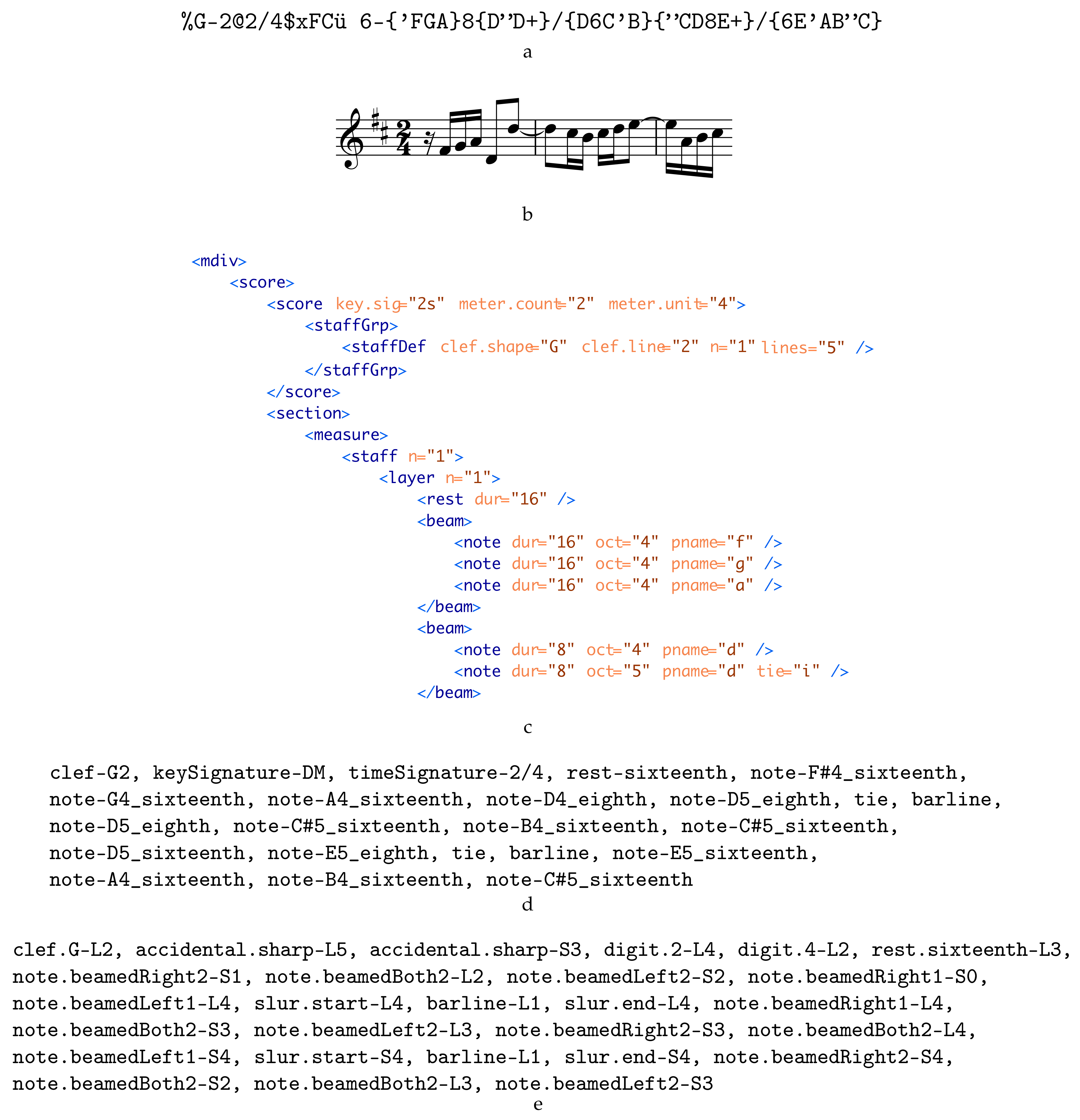
PrIMuS contains $87678$ real-music incipits (an incipit is a sequence of notes, typically the first ones, used for identifying a melody or musical work), each one represented by five files (see Figure 1): the Plaine and Easie code source [44], an image with the rendered score, the musical symbolic representation of the incipit both in Music Encoding Initiative format (MEI) [2] and in an on-purpose simplified encoding (semantic encoding), and a sequence containing the graphical symbols shown in the score with their position in the staff without any musical meaning (agnostic encoding). These two on-purpose agnostic and semantic representations, that will be described below, are the ones used in our experiments.

Currently, the biggest database of musical incipits available is RISM [5]. Created in 1952, the main aim of this organization is to catalog the location of musical sources. In order to identify musical works, they make use of the incipits of the contained pieces—as well as meta-data. To the date this article was written, the online version of RISM indexes more than 850,000 references, most of them monodic scores in CWMN. This content is freely available as an “Online public access catalog” (OPAC) (https://opac.rism.info). Due to the early origins of this repertoire, the musical encoding format used is Plaine and Easie Code (PAEC) [44].

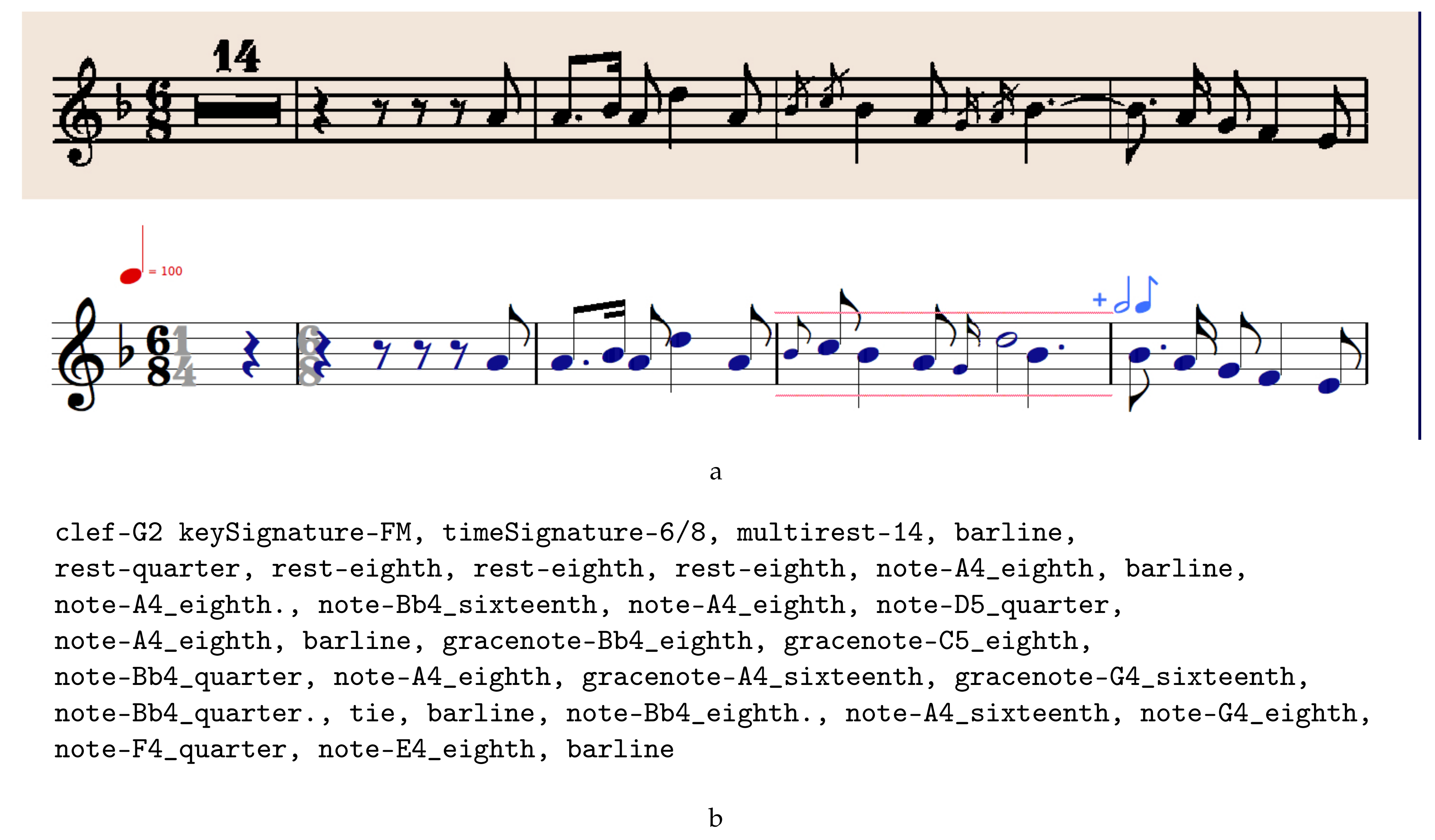
PrIMuS has been generated using as source an export from the RISM database. Given as input the PAEC encoding of those incipits (Figure 1a), it is formatted in order to feed the musical engraver Verovio [45] that outputs both the musical score (Figure 1b) in SVG format—that is posteriorly converted into PNG format—and the MEI encoding containing the symbolic semantic representation of the score in XML format (Figure 1c). Verovio is able to render scores using three different fonts, namely: Leipzig, Bravura, and Gootville. This capability is used to randomly choose one of the three fonts used in the rendering of the different incipits, leading to a higher variability in the dataset. Eventually, the on-purpose semantic and agnostic representations have been obtained as a conversion from the MEI files.

Semantic and Agnostic Representations

As introduced above, two representations have been devised on-purpose for this study, namely the semantic and the agnostic ones. The former contains symbols with musical meaning, e.g., a D Major key signature; the latter consists of musical symbols without musical meaning that should be eventually interpreted in a final parsing stage. In the agnostic representation, a D Major key signature is represented as a sequence of two “sharp” symbols. Note that from a graphical point of view, a sharp symbol in a key signature is the same as a sharp accidental altering the pitch of a note. This way, the alphabet used for the agnostic representation is much smaller, which allows us to study the impact of the alphabet size and the number of examples shown to the network for its training. Both representations are used to encode single staves as one-dimensional sequences in order to make feasible their use by the neural network models. For avoiding later assumptions on the behavior of the network, every item in the sequence is self-contained, i.e., no contextual information is required to interpret it. For practical issues, none of the representations is musically exhaustive, but representative enough to serve as a starting point from which to build more complex systems.

The semantic representation is a simple format containing the sequence of symbols in the score with their musical meaning (see Figure 1d). In spite of the myriad of monodic melody formats available in the literature [16], this on-purpose format has been introduced for making it easy to align it to the agnostic representation and grow-it in the future in the direction this research requires. As an example, the original Plaine and Easie code has not been directly used for avoiding its abbreviated writing that allows omitting part of the encoding by using previously encoded slices of the incipit. We want the neural network to receive a self-contained chunk of information for each musical element. Anyway, the original Plaine and Easie code and a full-fledged MEI file is maintained for each incipit that may be used to generate any other format. The grammar of the ground-truth files of the semantic representation is formalized in Appendix A (

Table A1. Lexical rules for the semantic grammar.

Token	Definition
digit	(‘0’..‘9’)
integer	(‘0’..‘9’)+
slash	‘.’
clefnote	{‘C’ | ‘G’ | ‘F’}
linenumber	{‘1’ | ‘2’ | ‘3’ | ‘4’ | ‘5’}
accidentals	{‘bb’ | ‘b’ | ‘n’ | ‘#’ | ‘x’}
metersigns	{“C” | “C/”}
trill	“trill”
fermata	“fermata”
clef	“clef”
note	“note”
gracenote	“gracenote”
rest	“rest”
multirest	“multirest”
barline	“barline”
thickbarline	“thickbarline”
figure	{”quadruple_whole” | “double_whole” | “whole” | “half” | “quarter” | “eighth” | “sixteenth”
	| “thirty_second” | “sixty_fourth” | “hundred_twenty_eighth” | “two_hundred_fifty_six”}
dot	‘.’
tie	“tie”
diatonicpitch	{‘A’ | ‘B’ | ‘C’ | ‘D’ | ‘E’ | ‘F’ | ‘G’}
keysignature	“keySignature”
timesignature	“timeSignature”
minor	‘m’
major	‘M’
sep	TAB
sepsymbol	’-’
sepvalues	‘_’

and

Table A2. Semantic file grammar.

sequence	→	(symbol sep symbol)*
symbol	→	clef sepsymbol clefnote linenumber
		$|$ timesignature sepsymbol (metersigns $|$ (integer slash integer))
		$|$ keysignature sepsymbol diatonicpitch accidentals? (major $|$ minor)?
		$|$ (note $|$ gracenote) sepsymbol pitch sepvalues figure dots? (sepvalues fermata)? (sepvalues trill)?
		$|$ tie
		$|$ barline
		$|$ rest sepsymbol figure dots? (sepvalues fermata)?
		$|$ multirest sepsymbol integer
pitch	→	diatonicpitch accidentals? octave
octave	→	integer
dots	→	dot+

).

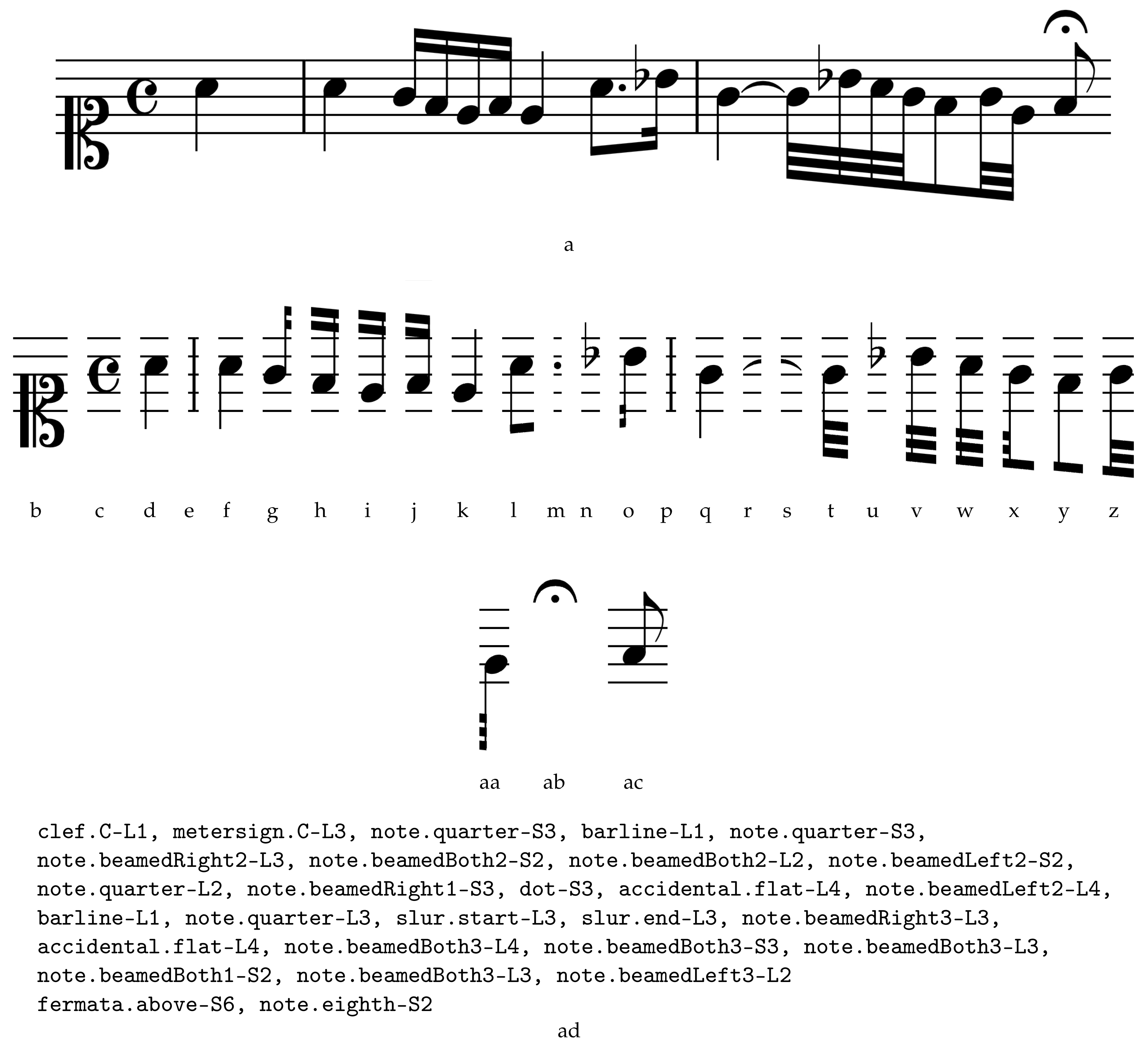
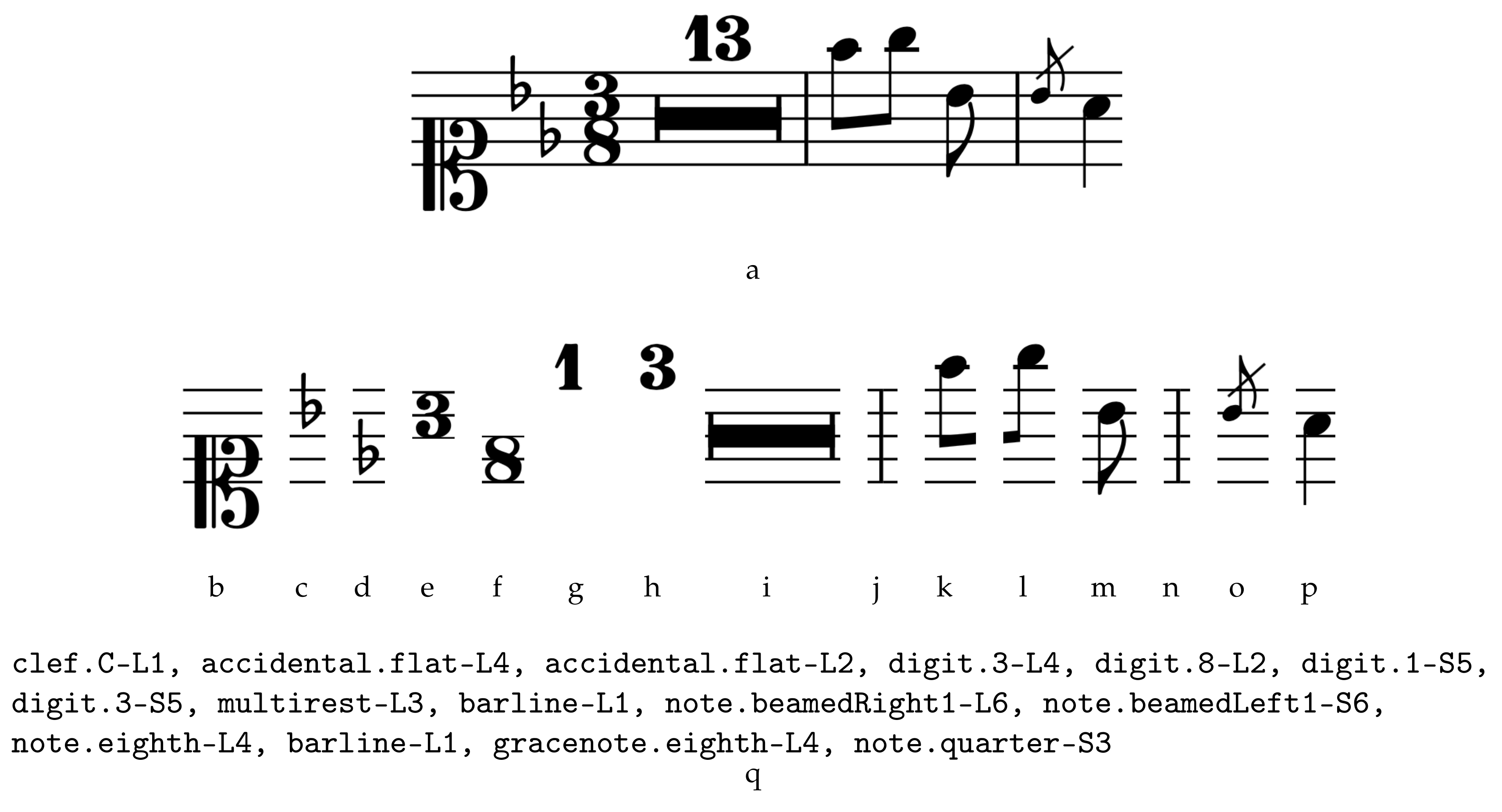
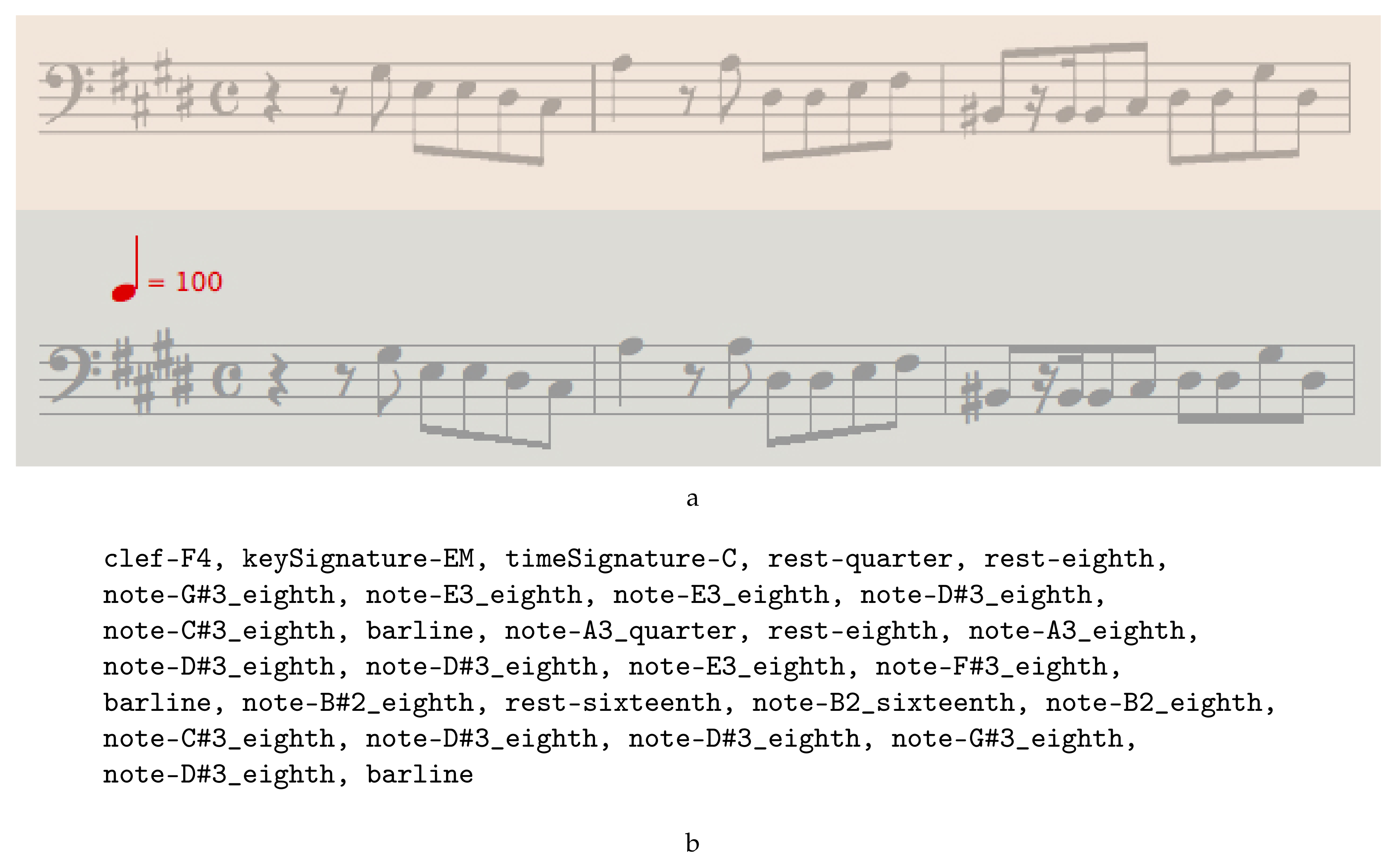
The agnostic representation contains a list of graphical symbols in the score, each of them tagged given a catalog of pictograms without a predefined musical meaning and located in a position in the staff (e.g., third line, first space). The Cartesian plane position of symbols has been encoded relatively, following a left-to-right, top-down ordering (see encoding of fractional meter inf Figure 1e). In order to represent beaming of notes, they have been vertically sliced generating non-musical pictograms (see Figure 2 and Figure 3). As mentioned above, this new way of encoding complex information in a simple sequence allows us to feed the network in a relatively easy way. The grammar of the ground-truth files of the agnostic representation is formalized in Appendix A (

Table A3. Lexical rules for the agnostic grammar.

Token	Definition
digit	(‘0’..‘9’)
integer	(‘0’..‘9’)+
clefnote	{‘C’ | ‘G’ | ‘F’}
accidentals	{“double_flat” | “flat” | “natural” | “sharp” | “double_sharp”}
metersigns	{“C” | “C/”}
startend	{“start” | “end”}
position	{“above” | “below”}
trill	“trill”
fermata	“fermata”
clef	“clef”
note	“note”
gracenote	“gracenote”
rest	“rest”
accidental	“accidental”
barline	“barline”
thickbarline	“thickbarline”
metersign	“metersign”
digit	“digit”
slur	“slur”
multirest	“multirest”
beams	{“beamLeft” | “beamBoth” | “beamRight”}
figures	{”quadruple_whole” | “double_whole” | “whole” | “half” | “quarter” | “eighth” | “sixteenth”
	| “thirty_second” | “sixty_fourth” | “hundred_twenty_eighth” | “two_hundred_fifty_six”}
sep	TAB
sepsymbol	‘.’
sepverticalposition	‘-’
linespace	{‘L’ | ’S’}

and

Table A4. Agnostic file grammar.

sequence	→	(symbol sep symbol)*
symbol	→	specificSymbol sepverticalpos verticalPos
verticalPos	→	linespace integer
specificSymbol	→	clef sepsymbol clefnote
		$|$ notesepsymbol (figure $|$ beam)
		$|$ rest sepsymbol figure
		$|$ accidental sepsymbol accidentals
		$|$ barline $|$ thickbarline
		$|$ metersign sepsymbol metersigns
		$|$ digit sepsymbol integer
		$|$ slur sepsymbol startend
		$|$ fermata sepsymbol position
		$|$ trill
		$|$ multirest
		$|$ gracenotesepsymbol (figure $|$ beam)
figure	→	figures
beam	→	beams digits

).

The agnostic representation has an additional advantage over the semantic one in a different scenario from that of encoding CWMN. In other less known musical notations, such as the early neumatic and mensural notations, or in the case of non-Western notations, it may be easier to transcribe the manuscript it two stages: one stage performed by any non-musical expert that only needs to identify pictograms, and a second stage where a musicologist, maybe aided by a computer, interprets them to yield a semantic encoding.

Although both representations can be considered equivalent, each representation does need a different number of symbols to codify the same staff. This also affects the size of their specific vocabularies. To illustrate this issue, we show in

Table 2. Composition of PrIMuS dataset in terms of number of samples (staves), size of the alphabet, and number of symbols with respect to the different representations.

	Agnostic	Semantic
Number of staves	87,678	87,678
Alphabet size	758	1781
Music symbols	2,397,824	2,095,836

an overview of the composition of PrIMuS with respect to the considered representations.

4. Neural End-to-end Approach for Optical Music Recognition

We describe in this section the neural models that allow us to face the OMR task in an end-to-end manner. In this case, a monodic staff section is assumed to be the basic unit; that is, a single staff will be processed at each moment.

Formally, let $\mathcal{X}=\{(x_1,y_1),(x_2,y_2),...\}$ be our end-to-end application domain, where $x_i$ represents a single staff image and $y_i$ is its corresponding sequence of music symbols. On the one hand, an image x is considered to be a sequence of variable length, given by the number of columns. On the other hand, y is a sequence of music symbols, each of which belongs to a fixed alphabet set $\Sigma$.

Given an input image x, the problem can be solved by retrieving its most likely sequence of music symbols $\widehat{y}$:

$$\widehat{y}=arg\underset{y\in {\Sigma }^{\ast }}{max}P\left(y\right|x)$$

(1)

In this work, the statistical framework is formulated as regards Recurrent Neural Network (RNN), as they represent neural models that allows working with sequences [46]. Ultimately, therefore, the RNN will be responsible of producing the sequence of musical symbols that fulfills Equation (1). However, we first add a Convolutional Neural Network (CNN), that is in charge of learning how to process the input image [47]. In this way, the user is prevented from fixing a feature extraction process, given that the CNN is able to learn to extract adequate features for the task at issue.

Our work is conducted over a supervised learning scenario; that is, it is assumed that we can make use of a known subset of $\mathcal{X}$ with which to train the model. Since both types of networks represent feed-forward models, the training stage can be carried out jointly, which leads to a Convolutional Recurrent Neural Network (CRNN). This can be implemented easily by connecting the output of the last layer of the CNN with the input of the first layer of the RNN, concatenating all the output channels of the convolutional part into a single image. Then, columns of the resulting image are treated as individual frames for the recurrent block.

In principle, the traditional training mechanisms for a CRNN force to provide the expected output in each output frame. However, the restriction imposed above with respect to the end-to-end term refers to that, for each staff, the training set only provides its corresponding sequence of expected symbols, without any kind of explicit information about the location of the semantic or agnostic symbols in the image. This scenario can be nicely solved by means of the CTC loss function [15].

Basically, CTC provides a means to optimize the CRNN parameters so that it is likely to give the correct sequence y given an input x. In other words, given the input x and its corresponding transcript y, CTC directly optimizes $P\left(y\right|x)$. Although optimizing this likelihood exhaustively is computationally unfeasible, CTC performs a local optimization using an Expectation-Maximization algorithm similar to that used for training Hidden Markov Models [48].

The CTC loss function is used only for training. At the decoding stage, one has to take into account the output provided by the CRNN, which still predicts a symbol for each frame (column) of the convoluted image. However, the way in which the network is trained allows a straightforward decoding. To indicate a separation between symbols, or to handle those frames in which there is no symbol, CTC considers an additional symbol in the alphabet that indicates this situation (blank symbol).

Note that the model is not expected to provide information about the location of the symbols in the decoding stage because of the way it is trained. Anyway, from a musical perspective, it is not necessary to retrieve the exact position of each music symbol in the image but their context in order to correctly interpret it.

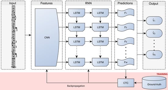
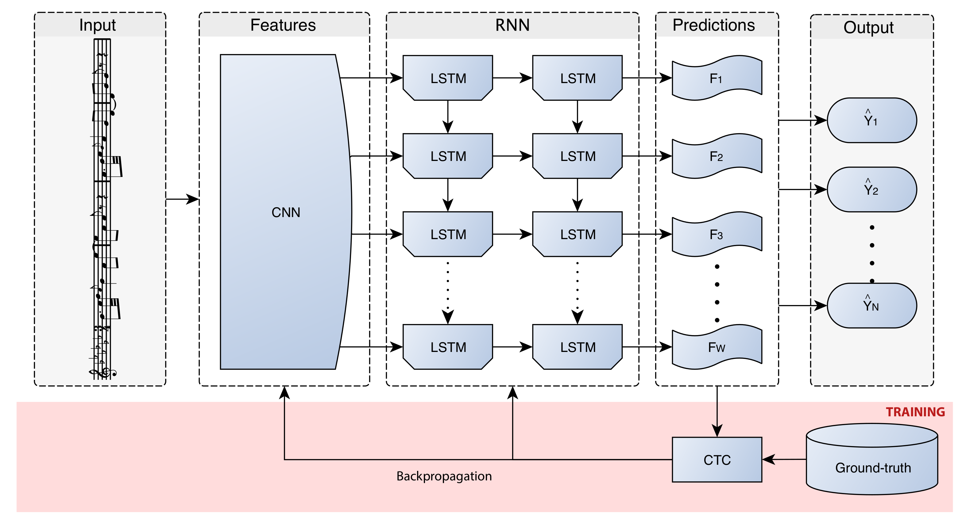
A graphical scheme of the framework is given in Figure 4. The details for its implementation is provided in the following sections.

Implementation Details

The objective of this work is not to seek the best neural model for this task, but to study the feasibility of this framework. Thus, a single neural model is proposed that, by means of informal testing, has verified its goodness for the task.

The details concerning the configuration of the neural model are given in

Table 3. Instantiation of the CRNN used in this work, consisting of 4 convolutional layers and 2 recurrent layers. Notation: Input$(h\times w\times c)$ means an input image of height h, width w and c channels; Conv$(n,h\times w)$ denotes a convolution operator of n filters and kernel size of $h\times w$; MaxPooling$(h\times w)$ represents a down-sampling operation of the dominating value within a window of size $(h\times w)$; BLSTM(n) means a bi-directional Long Short-Term Memory unit of n neurons; Dense(n) denotes a dense layer of n neurons; and Softmax() represents the softmax activation function. $\Sigma$ denotes the alphabet of musical symbols considered.

Input $(128\times \mathit{W}\times 1)$
Convolutional Block
Conv$(32,3\times 3)$, MaxPooling$(2\times 2)$
Conv$(64,3\times 3)$, MaxPooling$(2\times 2)$
Conv$(128,3\times 3)$, MaxPooling$(2\times 2)$
Conv$(256,3\times 3)$, MaxPooling$(2\times 2)$
Recurrent block
BLSTM$\left(256\right)$
BLSTM$\left(256\right)$
Dense$\left(\right|\Sigma |+1)$
Softmax$\left(\right)$

. As observed, input variable-width single-channel images (grayscale) are rescaled at a fixed height of 128 pixels, without modifying their aspect ratio. This input is processed through a convolutional block inspired by a VGG network, a typical model in computer vision tasks [49]: four convolutional layers with an incremental number of filters and kernel sizes of $3\times 3$, followed by the max-pool $2\times 2$ operator. In all cases, Batch Normalization [50] and Rectified Linear Unit activations [51] are considered.

At the output of this block, two recurrent bidirectional layers of 256 neurons, implemented as LSTM units [52], try to convert the resulting filtered image into a discrete sequence of musical symbols that takes into account both the input sequence and the modeling of the musical representation. Note that each frame performs a classification, modeled with a fully-connected layer with as many neurons as the size of the alphabet plus 1 (the blank symbol necessary for the CTC function). The activation of this neurons is given by a softmax function, which allows interpreting the output as a posterior probability over the alphabet of music symbols [53].

The learning process is carried out by means of stochastic gradient descent (SGD) [54], which modifies the CNN parameters through back-propagation to minimize the CTC loss function. In this regard, the mini-batch size is established to 16 samples per iteration. The learning rate of the SGD is updated adaptively following Adadelta algorithm [55].

Once the network is trained, it is able to provide a prediction in each frame of the input image. These predictions must be post-processed to emit the actual sequence of predicted musical symbols. Thanks to training mechanism with the CTC loss function, the final decoding can be performed greedily: when the symbol predicted by the network in a frame is the same as the previous one, it is assumed that they represent frames of the same and only only one symbol is concatenated to the final sequence. There are two ways to indicate a new symbol is predicted: either the predicted symbol is different from the previous frame or the predicted symbol of a frame is the blank symbol, which indicates that no symbol is actually found.

Thus, given an input image, a discrete musical symbol sequence is obtained. Note that the only limitation is that the output cannot contain more musical symbols than the number of frames of the the input image, which in our case is highly unlikely to happen.

5. Experiments

5.1. Experimental Setup

Concerning evaluation metrics, there is an open debate on which metrics should be used in OMR [10]. This is especially arguable because of the different points of view that the use of its output has: it is not the same if the intention of the OMR is to reproduce the content or to archive it in order to build a digital library. Here we are only interested in the computational aspect itself, in which OMR is understood as a pattern recognition task. So, we shall consider metrics that, even assuming that they might not be optimal for the purpose of OMR, allow us to draw reasonable conclusions from the experimental results. Therefore, let us consider the following evaluation metrics:

• Sequence Error Rate (%): ratio of incorrectly predicted sequences (at least one error).
• Symbol Error Rate (%): computed as the average number of elementary editing operations (insertions, modifications, or deletions) needed to produce the reference sequence from the sequence predicted by the model.

Note that the length of the agnostic and semantic sequences are usually different because they are encoding different aspects of the same source. Therefore, the comparison in terms of Symbol Error Rate, in spite of being normalized (%), may not be totally fair. Furthermore, the Sequence Error Rate allows a more reliable comparison because it only takes into account the perfectly predicted sequences (in which case, the outputs in different representations are equivalent).

Below we present the results achieved with respect to these metrics. In the first series of experiments we measure the performance that neural models can achieve as regards the representation used. First, they will be evaluated in an ideal scenario, in which a huge amount of data is available. Therefore, the idea is to measure the glass ceiling that each representation may reach. Next, the other issue to be analyzed is the complexity of the learning process as regards the convergence of the training process and the amount of data that is necessary to learn the task. Finally, we analyze the ability of the neural models to locate the musical symbols within the input staff, task for which it is not initially designed.

For the sake of reproducible research, source code and trained models are freely available [56].

5.2. Performance

We show in this section the results obtained when the networks are trained with all available data. This means that about 80,000 training samples are available, $10\%$ of which are used for deciding when to stop training and prevent overfitting. The evaluation after a 10-fold cross validation scheme is reported in

Table 4. Evaluation metrics with respect to the representation considered. Results reported represent averages from a 10-cross validation methodology.

	Representation
	Agnostic	Semantic
Sequence Error Rate (%)	17.9	12.5
Symbol Error Rate (%)	1.0	0.8

.

Interestingly, the semantic representation leads to a higher performance than the agnostic representation. This is clearly observed in the sequence-level error (12.5% versus 17.9%), and somewhat to a lesser extent in the symbol-level error (0.8% versus 1.0%).

It is difficult to demonstrate why this might happen because of the way these neural models operate. However, it is intuitive to think that the difference lies in the ability to model the underlying musical language. At the image level, both representations are equivalent (and, in principle, the agnostic representation should have some advantage). On the contrary, the recurrent neural networks may find it easier to model the linguistic information of the musical notation from its semantic representation, which leads—when there is enough data, as in this experiment—to produce sequences that better fit the underlying language model.

In any case, regardless of the selected representation it is observed that the differences between the actual sequences and those predicted by the networks are minimal. While it cannot be guaranteed that the sequences are recognized with no error (only 12.5% at best), the results can be interpreted as that only around 1% of the symbols predicted need correction to get the correct transcriptions of the images. Therefore, the goodness of this complete approach is demonstrated, in which the task is formulated in an elegant way in terms of input and desired output.

Concerning computational cost we would like to emphasize that although the training of these models is expensive—in the order of several hours over high-performance Graphical Processing Units (GPUs)— the prediction stage allows fast processing. It takes around 1 second per score in a general-purpose computer like an Intel Core i5-2400 CPU at 3.10 GHz with 4 GB of RAM, and without speeding-up the computation with GPUs. We believe that this time is appropriate for allowing a friendly usability in an interactive application.

5.2.1. Error Analysis

In order to dig deeper into the previously presented results, we conducted an analysis of the typology of the errors produced. The most repeated errors for each representation are reported in

Table 5. List of the 3 most common errors with respect to the representation considered. Percentages are relative to the total error rates from Table 4.

Rank	Representation
	Agnostic			Semantic
	Symbol	Percentage		Symbol	Percentage
# 1	barline-L1	45.5%		barline	38.6%
# 2	gracenote.sixteenth-L4	1.8%		tie	9.4%
# 3	accidental.natural-S3	1.4%		gracenote.C5-sixteenth	1.5%

.

In both cases, the most common error is the barline, with a notable difference with respect to the others. Although this may seem surprising at first, it has a simple explanation: the incipits often end without completing the bar. This, at the graphic level, hardly has visible consequences because the renderer almost always places the last barline at the end of the staff (most of the incipits contain complete measures). Thus, the responsibility of discerning whether there should be a barline or not lies almost exclusively in the capacity of the network to take into account “linguistic” information. The musical notation is a language that, in spite of being highly complex to model in its entirety, has certain regularities with which to exploit the performance of the system, as for instance the elements that lead to a complete measure. According to the results presented in the previous section, we can conclude that a semantic representation, in comparison with the agnostic one, makes it easier for the network to estimate such regularities. This phenomenon is quite intuitive, and may be the main cause of the differences between the representations’ performance.

As an additional remark, note that both representations miss on grace notes, which clearly represent a greater complexity in the graphic aspect, and are worse estimated by the language model because of being less regular than conventional notes.

In the case of the semantic representation, another common mistake is the tie. Although we cannot demonstrate the reason behind these errors, it is interesting to note that the musical content generated without that symbol is still musically correct. Therefore, given the low number of tie symbols in the training set (less than 1%), the model may tend to push the recognition towards the most likely situation, in which the tie does not appear.

5.2.2. Comparison with Previous Approaches

As mentioned previously, the problem with existing scientific OMR approaches is that they either focus only on a sub-stage of the process (staff-line removal, symbol classification, etc.) or are heuristically developed to solve the task in a very specific set of scores. That is why we believe it would be quite unfair to compare these approaches with ours, the first one that covers a complete workflow exclusively using machine learning.

As an illustrative example of this matter, we include here a comparison of the performance of our approach with that of Audiveris (cf. Section 2) over PrIMuS, even assuming in advance that such comparison is not fair. As a representative of our approach, we consider the semantic representation, given that the output of Audiveris is also semantic (the semantic encoding format has been obtained from the Audiveris MusicXML batch-mode output).

Table 6. Quantitative comparison with respect to accuracy (Symbol Error Rate in%) and processing time (avg. seconds per sample) between our CRNN-based approach and Audiveris. Values in bold highlight the best results in each metric.

	Symbol Error Rate (%)	Avg. s per Sample
CRNN	0.8	1
Audiveris	44.2	15

reports the accuracy with respect to the Symbol Error Rate attained, as a general performance metric, and the computational time measured as seconds per sample, from both our approach and Audiveris.

It can be observed that Audiveris, which surely works well in certain types of scores, is not able to offer a competitive accuracy in the corpus considered, as it obtains an SER above 40%. Additionally, the computation time is greater than ours under the same aforementioned hardware specifications, which validates the CRNN approach in this aspect as well.

5.3. Learning Complexity

The vast amount of available data in the previous experiment prevents a more in-depth comparison of the representations considered. In most real cases, the amount of available data (or the complexity of it) is not so ideal. That is why in this section we want to analyze more thoroughly both representations in terms of the learning process of the neural model.

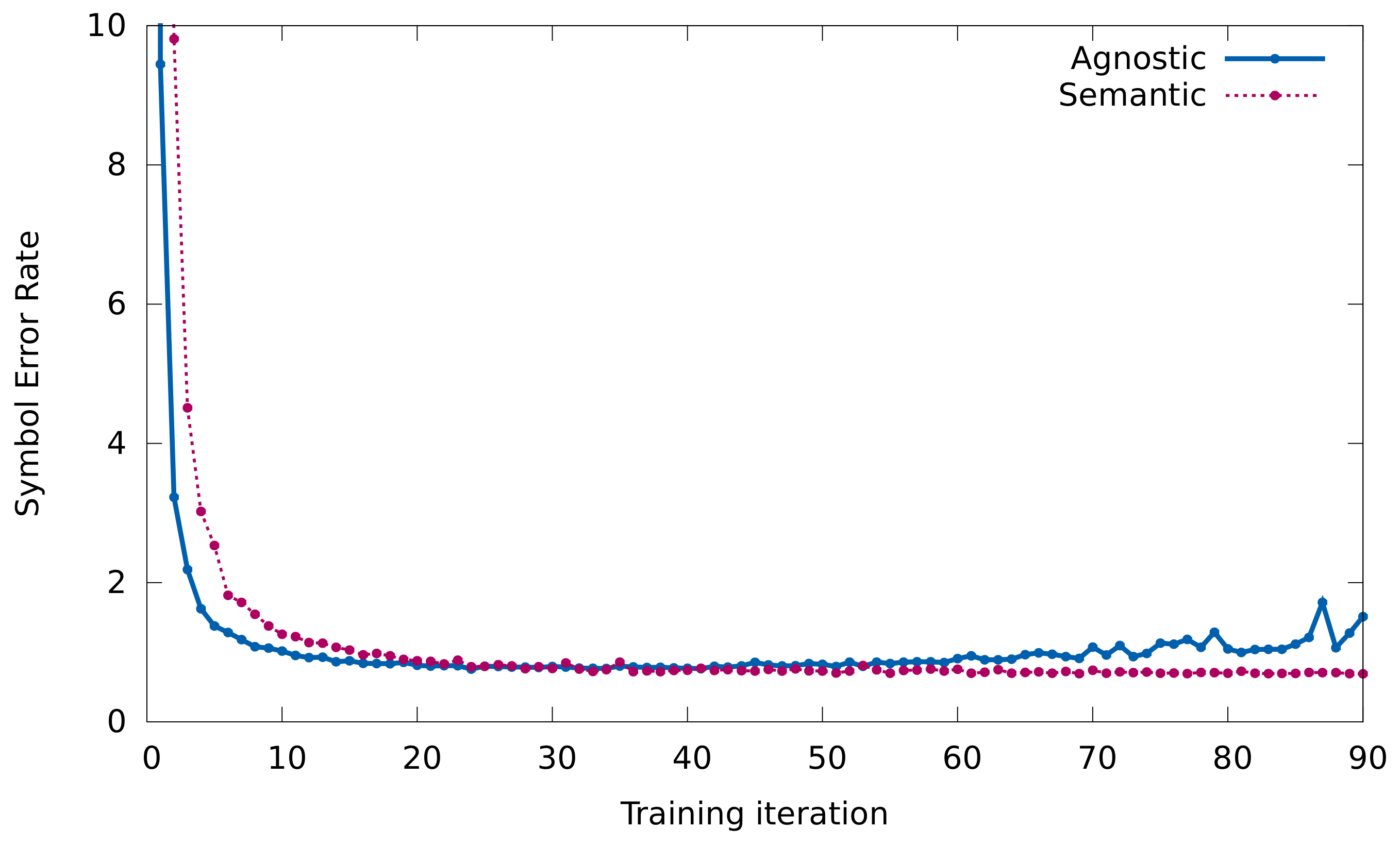
First, we want to see the convergence of the models learned in the previous section. That is, how many training epochs the models need for tuning their parameters appropriately. The curves obtained by each type of model are shown in Figure 5.

From these curves we can observe two interesting phenomena. On the one hand, both models converge relatively quick, as after 20 epochs the elbow point has already been produced. In fact, the convergence is so fast that the agnostic representation begins to overfit around the 40th epoch. On the other hand, analyzing the values in further detail, it can be seen that the convergence of the model that trains with the agnostic representation is more pronounced. This could indicate a greater facility to learn the task.

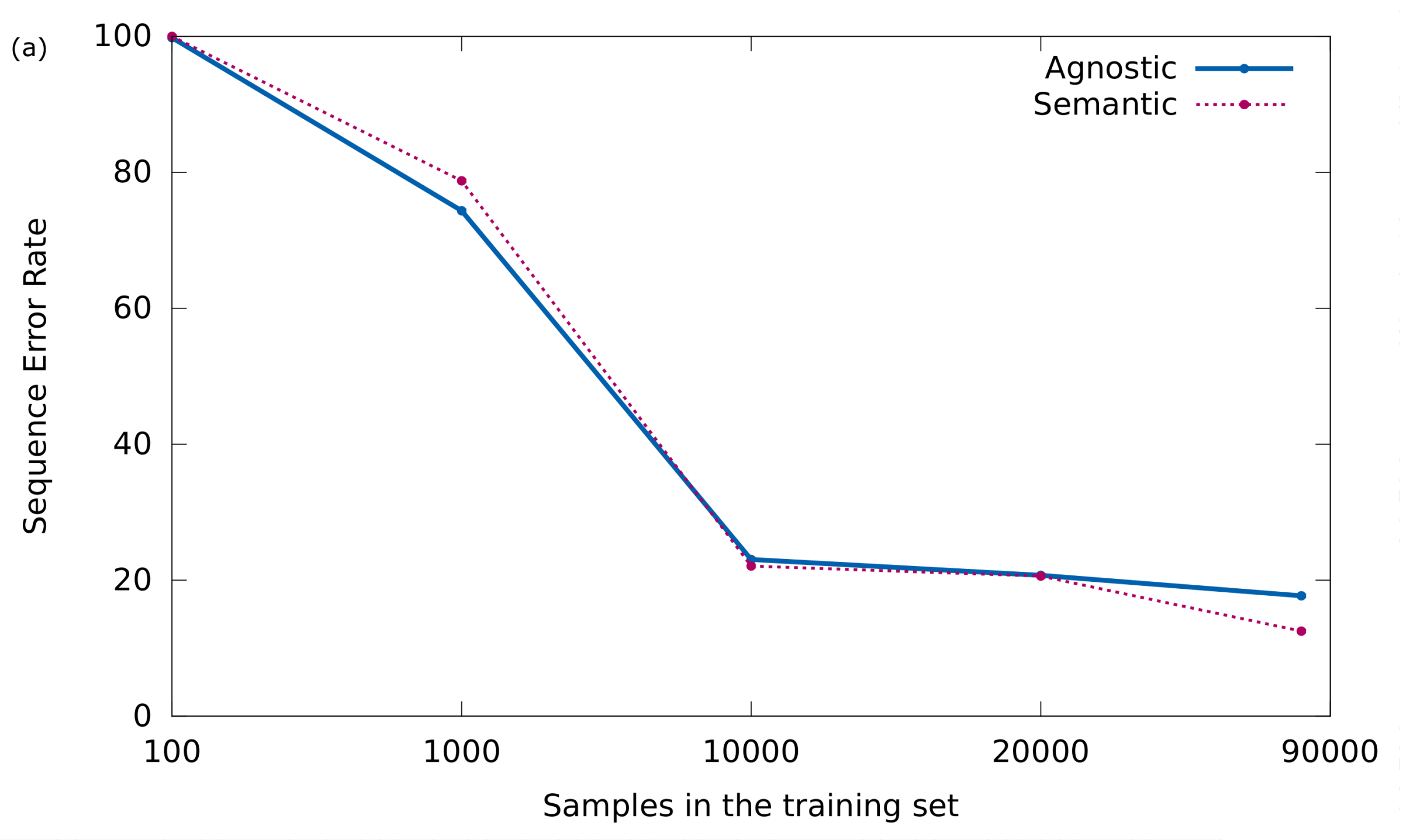
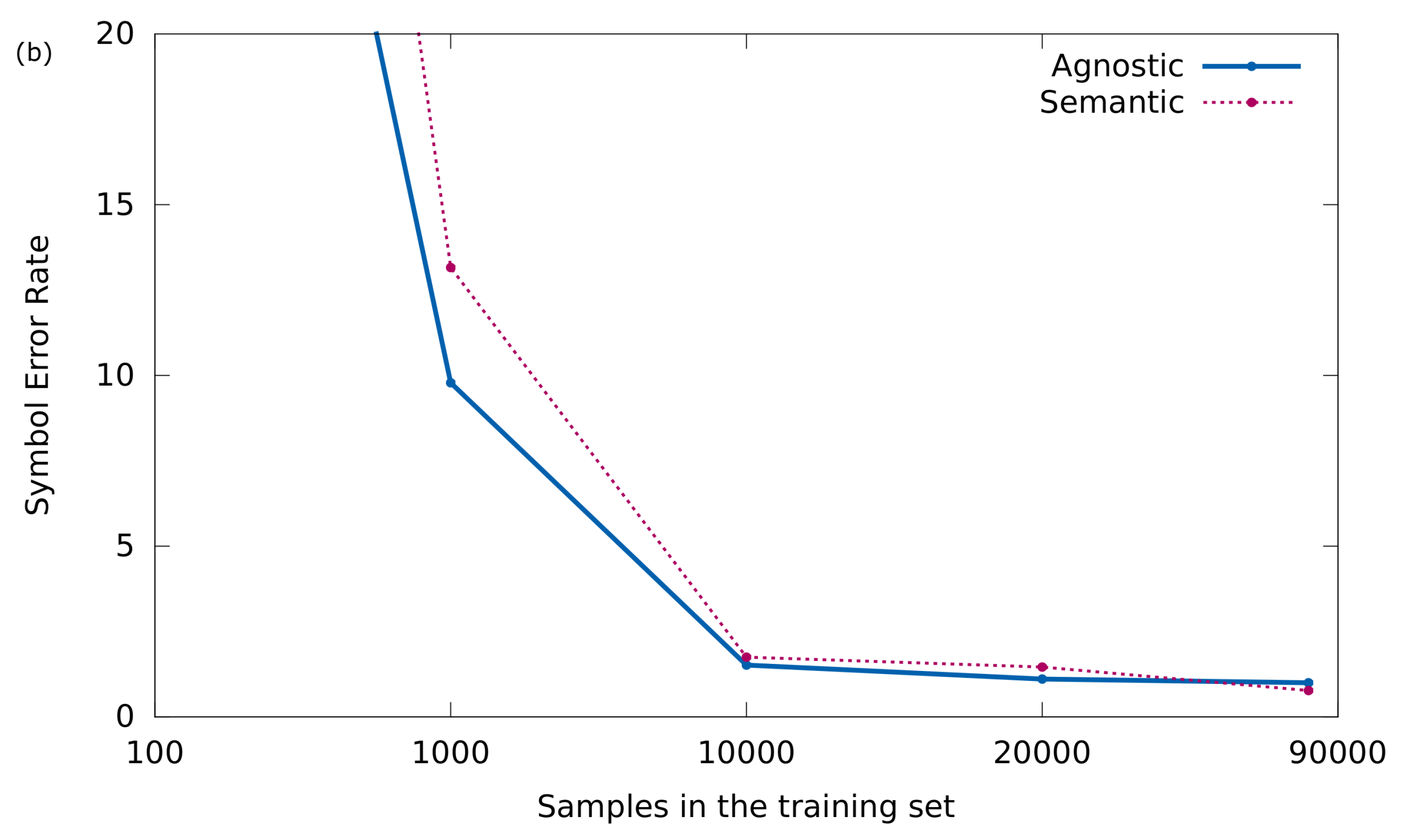
To confirm this phenomenon, the results obtained in an experiment in which the training set is incrementally increased are shown below. In particular, the performance of the models will be evaluated according to the size of training set sizes of 100, 1000, 10,000, and 20,000 samples. In addition, in order to favor the comparison, the results obtained in Section 5.2 will be drawn in the plots (around 80,000 training samples).

The evolution of both Sequence and Symbol Error Rate are given in Figure 6a,b, respectively, for the agnostic and semantic representations.

These curves certify that learning with the agnostic model is simpler, because when the number of training samples is small, this representation achieves better results.

We have already shown that, in the long run, the semantic representation slightly outperforms its performance. However, these results may give a clue as to which representation to use when the scenario is not so ideal like the one presented here. For example, when either there is not so much training data available or the input documents depict a greater difficulty (document degradation, handwritten notation, etc.).

5.4. Localization

As already mentioned above, the CTC loss function has the advantage that it allows to train the model without needing an aligned ground-truth; that is, the model does not need to know the location of the symbol within the input image. In turn, this condition is a drawback when the model is expected to infer the positions of the symbols in the image during decoding. The CTC function only worries that the model converges towards the production of the expected sequences, and ignores the positions in which the symbols are produced.

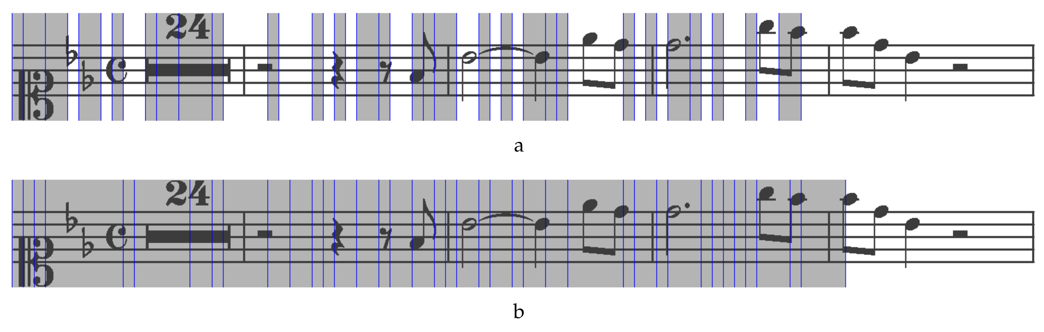
We show in Figure 7 an image that is perfectly predicted by our approach, both in the agnostic (Figure 7a) and semantic (Figure 7b) case. We have highlighted (in gray) the zones in which the network predicts that there is a symbol, indicating with blue lines the boundaries of them. The non-highlighted areas are those in which the blank symbol is predicted.

In both cases it can be clearly observed that the neuronal model hardly manages to predict the exact location of the symbols. It could be interpreted that the semantic model has a slightly better notion—since it spans better the width of the image—but it does not seem that such information is useful in practice unless the approximate position is enough for the task using it.

This fact, however, is not an obstacle to correctly predict the sequence since the considered recurrent block is bidirectional; that is, it shares information in both directions of the x-dimension. Therefore, it is perfectly feasible to predict a symbol in a frame prior to those in which it is actually observed.

5.5. Commercial OMR Tool Analysis

There exist many commercial OMR tools with which a comparison can be carried out. For this analysis, we choose one of the best commercial tools available: Photoscore Ultimate (www.neuratron.com/photoscore.htm), version 8.8.2. It is publicized as having “22 years” of recognition experience and accuracies “over 99.5%”. However, since Photoscore is conceived for its interactive use, it does not allow for batch processing. Therefore, the comparison of our approach with this tool will be conducted qualitatively by studying the behavior in some selected examples.

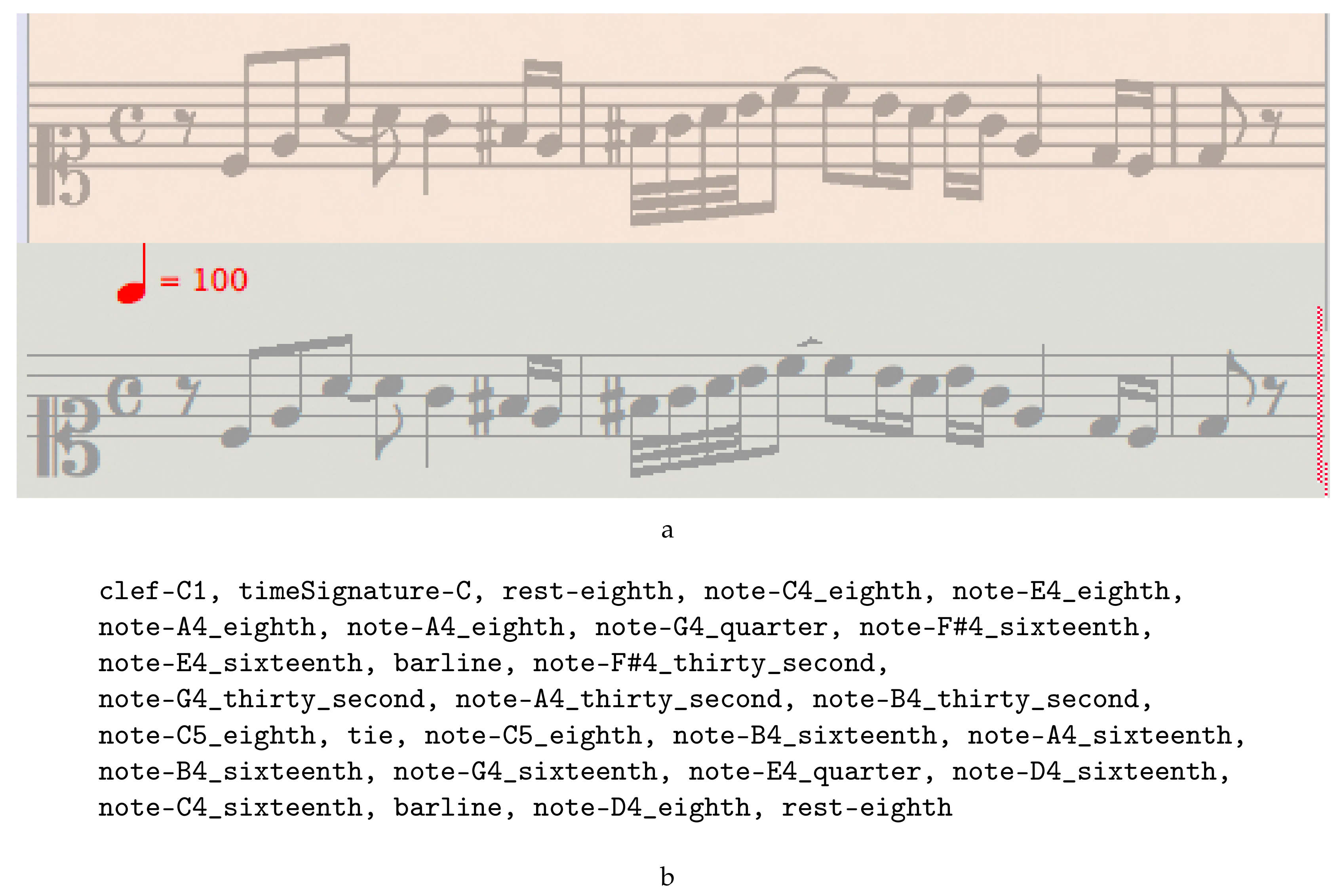
Images supplied to Photoscore have been converted into TIFF format with 8-bit depth, following the requirements of the tool. Below, we will show some snapshots of the output of the application, where the white spaces around the staves have been manually trimmed for saving space. Note that the output of Photoscore is not a list of recognized music glyphs, but the musical content itself. Thus, in its output, the tool superimposes some musical symbols that, despite being not present at the input image, indicate the musical context that the tool has inferred. Namely, these visual hints are time signatures drawn in gray, tempo marks in red, and musical figures preceded by a plus or a minus sign showing the difference between the sum of the figures actually present in the measure and the expected duration given the current time signature. From our side, we provide the sequence of music symbols predicted by our model so as to analyze the difference between both outputs.

For illustrating the qualitative comparison, we manually looked for samples that cover all possible scenarios. For instance, Figure 8b shows an incipit in which both systems fail, yet for different reasons: Photoscore misses the last appoggiatura, whereas our method predicts an ending barline that is not in the image (this error was already discussed in Section 5.2.1).

For the sample depicted in Figure 9, the output of Photoscore is exact, but our system misses the first tie. The opposite situation is given by the sample of Figure 10, where Photoscore makes many mistakes. It is not able to correctly recognize the tie between the last two measures. In addition, the acciaccaturas are wrongly detected: they are identified as either appoggiaturas or totally different figures such as eighth note or half note. On the contrary, our system perfectly extracts the content from the score.

Finally, the sample of Figure 11 is perfectly recognized by both Photoscore and our system.

The examples given above show some of the most representative errors found. During the search of these examples, however, it was difficult to find samples where both system failed. In turn, it was easy to find examples where Photoscore failed and our system did not. Obviously, we do not mean that our system behaves better than Photoscore, but rather that our approach is competitive with respect to it.

6. Conclusions

In this work, we have studied the suitability of the use of the neural network approach to solve the OMR task in an end-to-end fashion through a controlled scenario of printed single-staff monodic scores from a real world dataset.

The neural network used makes use of both convolutions and recurrent blocks, which are responsible of dealing with the graphic and sequential parts of the problem, respectively. This is combined with the use of the so-called CTC loss function that allows us to train the model in a less demanding way: only pairs of images and their corresponding transcripts, without any geometric information about the position of the symbols or their composition from simple primitives.

In addition to this approach, we also present the Printed Images of Music Staves (PrIMuS) dataset for use in experiments. Specifically, PrIMuS is a collection of $87678$ incipits extracted from the RISM repository and rendered with various fonts using the Verovio tool.

The main contribution of the present work consisted of analyzing the possible codifications that can be considered for representing the expected output. In this paper we have proposed and studied two options: an agnostic representation, in which only the graphical point of view is taken into account, and a semantic representation, which codifies the symbols according to their musical meaning.

Our experiments have reported several interesting conclusions:

• The task can be successfully solved using the considered neural end-to-end approach.
• The semantic representation that includes musical meaning symbols has a superior glass ceiling of performance, visibly improving the results obtained using the agnostic representation.
• In general, errors occur in those symbols with less representation in the training set.
• This approach allows a performance comparable to that of commercial systems.
• The learning process with the agnostic representation made up of just graphic symbols is simpler, since the neural model converges faster and the learning curve is more pronounced than those with the semantic representation.
• Regardless of the representation, the neural model is not able to locate the symbols in the image—which could be expected because of the way the CTC loss function operates.

As future work, this work opens many possibilities for further research. For instance, it would be interesting to study the neural approach in a more general scenario in which the scores are not perfectly segmented into staves or in non-ideal conditions at the document level (irregular lighting, geometric distortions, bleed-through, etc.). However, it is undoubted that the most promising avenue is to extend the neural approach so that it is capable of dealing with a comprehensive set of notation symbols, including articulation and dynamic marks, as well as with multiple-voice polyphonic staves. We have seen in PrIMuS that there are several symbols that may appear simultaneously (like the numbers of a time signature), and the neural model is able to deal with them. However, it is clear that polyphony, both at the single staff level (eg., chords) or at the system level, represents the main challenge to advance in the OMR field. Concerning the most technical aspect, it would be interesting to study a multi-prediction model that uses all the different representations at the same time. Given the complementarity of these representations, it is feasible to think of establishing a synergy that ends up with better results in all senses.