Abstract
This study presents a new adaptive trajectory tracking control scheme for a fully actuated Unmanned Surface Vehicle (USV) to track a common moving target region. In this control concept, the desired objective trajectory is specified as a moving region instead of a moving point, and so which is called non-strict trajectory tracking. Within this control scheme, a regression matrix is used to handle the parameter uncertainties, and region-based control scheme is used to track a desired moving region. A switching gain control term based on the exponential function is proposed to make the USV’s trajectory converge into the desired moving region rather than converge on the boundary of the moving region, and to reduce system chattering at the same time. A Lyapunov-like function is presented for stability analysis of the proposed control scheme. Numerical simulations are conducted to demonstrate the performance of the proposed non-strict trajectory tracking control scheme of the USV.
1. Introduction
Nearly two-thirds of the Earth is covered by oceans but only a few areas have been thoroughly explored. Unmanned marine vehicles are suitable for developing marine resources. Over the past decade, the increasing worldwide interest in military reconnaissance, homeland security, shallow-water surveys, environmental monitoring, and commercial and scientific issues associated with oceans has resulted in the increase in demand for the development of unmanned surface vehicles (USVs) with advanced control capabilities [1].
USVs are usually controlled remotely by humans; thus, an effective and reliable guidance, navigation, and control system for the autonomous sailing of USVs is important. Trajectory tracking is a typical motion control problem for USVs, which is considered with the design of control schemes that force a USV to reach and follow a time parameterized reference trajectory.
In the past few decades considerable research efforts have been devoted to the trajectory tracking problem of ships or USVs. Pettersen and Nijmeijer [2] transformed a model into a triangular-like form through a coordinate transformation to use integrator backstepping in developing a tracking control law for an underactuated ship. In [3], the authors presented a solution based on previous work by Hindman and Hauser to the problem of combined trajectory tracking and path following for fully actuated autonomous marine vehicles with non-negligible dynamics. A multivariable sliding-mode control (SMC) law was proposed for the trajectory tracking problem on the basis of nonlinear horizontal motion dynamics of a class of marine vessels in [4]; the ship positions and yaw angle were simultaneously tracked well. In [5], the USV could track desired arbitrary trajectories using a nonlinear robust model-based sliding mode approach; experiments demonstrated that the method was effective. In [6], the authors designed a novel trajectory tracking robust controller through a vectoral backstepping technique with an observer to provide an estimation of unknown disturbances; the proposed trajectory tracking control scheme could provide good transient and steady-state performance for the considered ship system. To realize the trajectory planning and tracking of a USV, the trajectory tracking control law in [7] was based on an SMC approach, and the trajectory of the USV finally converged into the desired target trajectory well. The hydrodynamic coefficients of the surface ship at high speed are difficult to be accurately estimated first; thus, in [8], the author proposed an adaptive output feedback controller based on neural network feedback–feedforward compensator in controlling a surface ship at high speed to track a desired trajectory. A novel trajectory following controller for underactuated surface vessels based in Active Disturbance Rejection Control (ADRC) technique was proposed in [9]. The accurate straight line and curve trajectory tracking for USV were realized using this controller. In order to implement high-speed trajectory tracking tasks for USVs, the authors in [10] put forward a line of sight (LOS) guidance algorithm based on the SF (Serret-Frenet) coordinates framework (SFLOS) and bio-inspired algorithm. In [11], the authors used the non-singular terminal sliding mode control technique and a robust homogeneous differentiator to propose a finite-time trajectory tracking control approach for an USV with unknown dead-zones and unknown disturbances. Using the method, the USV can reduce chattering and track the desired trajectory effectively. In [12], addressed through an integral sliding mode control and homogeneous disturbance observer, a finite-time trajectory tracking control of USV is proposed, considering input saturations and unknown disturbances. Using this control scheme, the actual trajectory can track precisely the desired trajectory and tracking errors can be rendered to zero in a finite time. Combining an adaptive fuzzy backstepping technique with Nussbaum approach, the researchers in [13] proposed a novel Nussbaum-based adaptive fuzzy control scheme for trajectory tracking of a USV in the presence of complex unknown nonlinearities and fully unknown dynamics, and tracking errors can converge to an arbitrarily small neighborhood of zero using this method. In [14], the authors proposed an estimator-based backstepping controller to control the unmanned surface ship to follow a desired trajectory considering external disturbance and system uncertainty, and the estimator was used to precisely estimate external disturbance and system uncertainties, which guaranteed that the desired trajectory can be followed with an exponential rate of convergence. A novel model based backstepping controller was designed in [15] for trajectory tracking control of underactuated USV, in which the well-known persistent exciting conditions of yaw velocity was completely relaxed; the USV could track an arbitrary trajectory, including a circle, straight-line and generally curved trajectories. In [16], an adaptive robust controller proposed by hierarchical sliding mode and a neural network was used for trajectory tracking and stabilization of underactuated surface vessels.
From the above review we can see that previous research about the trajectory tracking problem of USVs have motivated researchers to proposed different control methods, such as SMC, backstepping technique, Lyapunov’s direct method, robust control method and hybrid control technology. However, in [2,3,4,5,6,7,8,10,15], though different traditional methods were conducted, many of them didn’t consider the parameter uncertainties or disturbances. In [9], the author considered disturbance rejection, but control inputs were not analyzed. In [11,12,13,14,16], novel strategies were proposed considering parameter uncertainties or disturbances, and they were effective for the trajectory tracking of USVs. However, in most of the recent studies, USVs or ships are required to follow a specified path or track a predefined position strictly. Unlike the specified path or trajectory tracking of the previous researches, in this study, the proposed strategy is conducted to control the USV to track a moving regional trajectory rather than move along a pre-defined trajectory strictly.
We know that, in practice, some missions of USVs or ships do not require a strict point or a strictly particular path. For example, a USV sailing through a narrow waterway can be considered sailing through a region rather than a particular path. A USV or a ship sailing into a port can be regarded as sailing into a region rather than a strict point. Thus, when the USV or ship sails in the open sea, a strict trajectory tracking is unnecessary. For the trajectory tracking problem, one can consider control of a USV to track a common moving target region instead of a moving point. Then, the USV will track a region trajectory generated by the moving region. We call this problem a non-strict trajectory tracking. Figure 1 shows the concept of non-strict trajectory tracking. The USV can move into any place of the moving region trajectory rather than strictly moving along the pre-defined trajectory.
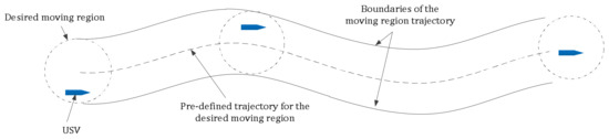
Figure 1.
Concept of non-strict trajectory tracking.
Cheah et al. [17,18] proposed a new region reaching concept for a robot manipulator and adopted similar concepts for an underwater vehicle in 2004 [19]. The desired region was specified by an objective function , where is the error in position leading to the region control (RC) problem. Sun [20] proposed a new region-reaching controller for an underwater vehicle mounted with a manipulator based on RC. Haghighi [21] used RC to control a swarm of robots to establish any arbitrary complex formation. Region-reaching tasks save energy and result in fast motion [18]. Region control is a good method for non-strict trajectory tracking. Some related works have been conducted in recent years. Li et al. [22] proposed an adaptive controller where the desired region is time varying and the region tracking control problem was solved instead of the region-reaching control problem. However, autonomous underwater vehicles (AUVs) consistently converge on the boundary of the region, which will cause AUV chattering when disturbances exist. Nonlinear H∞ and region-based control schemes in [23] are used to control an underwater vehicle to track a moving region. However, as long as the AUVs are inside the desired region, the control input is turned off; when the disturbances pull the vehicles out, the control input is turned on, which will cause input chattering. In [24], an adaptive region boundary-based concept was presented for an AUV, in which the controller was designed to allow the convergence of the vehicle to the boundary or a motionless region surface regardless of its initial position. In [25], the authors proposed a region tracking controller that guarantees an AUV to move within a region considering input delay.
In the present study, we propose a non-strict trajectory tracking scheme for a fully actuated USV to track a region trajectory. Based on a traditional RC method, a regression matrix is used to handle parameter uncertainties. Moreover, a switching gain control term based on the exponential function is proposed to make the USV’s trajectory converge into the desired moving region rather than the boundary of the moving region, thereby reducing system’s chattering, which is good for energy saving. The USV can follow a straight-line region trajectory, as well as a curved region trajectory, under the proposed controller. The traditional RC is used for a comparative study to illustrate further the performance of the proposed non-strict trajectory tracking control (NTTC).
2. Kinematics and Dynamic Models of USV
A USV moves in six degrees of freedom (6-DOF) with three translation displacements to define the location and three angular displacements to define the orientation. These motions are often described in two types of reference frame, namely the inertial and body-fixed frames. The motions in heave, roll, and pitch are neglected. The kinematics and dynamics of the USV without external environmental disturbances are described as follows [26]:
where
The system inertia matrix ; is a skew-symmetric matrix of Coriolis and centripetal terms; is the hydrodynamic damping matrix and it is strictly positive such that .
Here denotes the position in the heading angle of the USV in the earth-fixed frame; present the velocities of the USV in the body-fixed frame (surge velocity: , sway velocity: ; and yaw velocity: ); is the control input of the USV (surge force: , sway force: ; and yaw moment: ); is the mass of the USV; , , , , and are the added masses; is the -coordinate of the USV center of gravity in the body-fixed frame; and is the inertia with respect to the vertical axis. The coefficients , , , , , , , , , , , , , and are the hydrodynamic parameters of the USV.
For the actual USV, the velocities and input forces are limited. Thus, we make the following assumption.
Assumption: The input forces of the USV are bounded as , and with known bounds , and .
3. Control Strategy
This section presents the proposed control strategy. The proposed control strategy composes three parts. The region control term is the first part of the strategy. To control the USV to track a moving region, the region tracking errors will be first proposed using the desired moving region and the USV’s actual trajectory. Then the region control term is built by region tracking errors, which is the main part of the control strategy to make the USV track the desired moving region. An update law using a regression matrix is added to the region control term to handle the parameter uncertainties, which is the second part of the strategy. The third part is a switching gain control term based on the exponential function of the trajectory error, which is proposed to make the USV’s trajectory converge into the desired moving region rather than converge on the boundary of the moving region, and to reduce system chattering at the same time. The closed loop diagram of the controller structure is shown in Figure 2, and the symbols in it will be explained in the following sections. Next, the detailed design process of the proposed control strategy will be described.
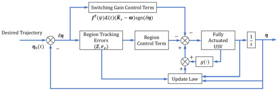
Figure 2.
Closed loop diagram of the controller structure.
3.1. Desired Region Description and Error Dynamics
In the region-based control framework, the desired moving target is specified by a region at the desired trajectory. Moreover, the USV must converge into the region. The desired region is specified by an inequality or by the objective function as
where is a scalar function with continuous first partial derivative, is the total number of objective function, and , . is the reference point of the desired region. , where is the total number of objective function. An illustration of the objective function is shown in Figure 3.
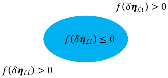
Figure 3.
Example of objective function.
is a time varying and nonsingular scaling factor. and are bounded functions of time. When the value of the scaling factor changes, the size of the desired region will also change, which allows the USV to track a time-varying moving region.
The USV moves in 3-DOF. Thus, we select . Then, the desired object function will be . The desired region can be defined as
where is the region boundary. A nonsingular matrix is defined as follows:
where , , and are the scaling factors of , , , respectively, and
The desired region decreases with the increase of the scaling factors, and vice versa.
The corresponding potential energy function for the desired region described in Equation (4) can be specified as
where is a positive scalar. That is:
Hence, the potential energy function can be defined as:
By partially differentiating the potential energy described by Equation (9) with respect to , we obtain
Equation (10) is represented as the region error in the following form:
3.2. Control Law Formulation
The control object is to control the USV tracking the moving target region, and to make the USV’s position and yaw converge into the desired regions. That is, the desired objective function (Equation (4)) always holds.
Based on the region error , a useful reference vector is defined as:
where is a positive constant, and . The matrix is the inverse of the rotation matrix . and are the time derivative and inverse of the scaling matrix , respectively.
On the basis of , , and the subsequent stability analysis, a filtered tracking error vector for the USV is defined as
The time derivative of is calculated as
where .
Then, the open loop error of the USV is expressed as follows:
where , is a vector of unknown parameters, and is a known regression matrix [27]. is the known part of . Furthermore,
The NTTC law can be proposed as:
where is a positive constant matrix. The estimated parameters are updated using the following update law:
where is a symmetric positive definite. The last term in Equation (15) is the switching gain control term.
In Equation (15), an exponential function is used to define , as shown as follows:
where , which satisfies the following inequation:
where ; is a positive number vector; and , , and . is also a positive number vector, where .
Equations (14) and (15) are combined. Then, the closed-loop dynamic equation of the USV is proposed as
3.3. Stability Analysis
A control Lyapunov function is defined as follows:
Then, Equation (19) is differentiated with respect to time, as shown as follows:
Given , then
Substituting Equation (11) into Equation (21), yields
where
Given , , then . So
where
and
Then, 3 cases are considered to discuss the convergence of in :
- Case 1:
- If , or , then will evidently converge to zero gradually.
- Case 2:
- If , then . does not hold if and only if , that is .
- Case 3:
- If , then . does not hold if and only if ; that is, .
By substituting into Equation (24), will eventually converge into , that is,
Substituting into yields . Then, combining Equation (25) results in the closed-loop system eventually converging into the desired region. Consequently, .
4. Simulation Results
Several computer simulations are performed to demonstrate the effectiveness of the control scheme proposed for non-strict trajectory tracking of the fully actuated USV. Here, the USV is ordered to track a moving region. The trajectory of the moving region is composed of a straight line and a sinusoidal curve. The traditional RC method is used for the comparative study to illustrate further the performance of the proposed NTTC method.
The CyberShip II (CS2) model from the Marine Cybernetics Laboratory (MCLab, Trondheim, Norway) of NTNU (Norwegian University of Science and Technology, Trondheim, Norway) is used for the simulations. CS2 is a 1:70 scale replica of a supply ship. Its mass is , its length is , and its breadth is . It is fully actuated with two main propellers, two aft rudders, and one bow thruster. The parameters of the vehicle, which are obtained from [28], are shown in Table 1.

Table 1.
Parameters of the USV.
The input forces of the USV are bounded as , and . The initial position of the USV is , , and the initial yaw is . The initial velocities of the USV are .
The trajectory of the desired moving region is specified as a straight line and a sinusoidal curve given by the following equations:
where , and . The desired yaw is set according the Line-of-Sight (LOS) guidance law [26] during the desired straight-line trajectory, and is set to be the tangential angle of the desired trajectory during the desired curved trajectory. The desired yaw is specified as follows:
The desired regional bounds of the desired moving region are expressed as , and the region scaling factor is .
The parameters of potential energy functions are . The positive constant parameter of the reference vector is expressed as . The parameters of the update law are selected as . The positive constant matrix of the control law is . The parameters of the switching gain control term are specified as and . The total simulation time is 2000 s. Figure 4, Figure 5, Figure 6, Figure 7, Figure 8, Figure 9, Figure 10, Figure 11 and Figure 12 show the simulation results.
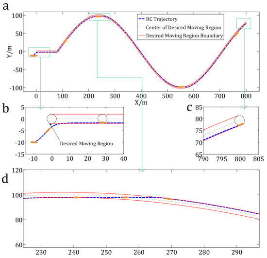
Figure 4.
Results of the traditional RC method. (a) Trajectory of the USV using the traditional RC method; (b) Zoom view of the results from −10 to 40 m in the X direction; (c) Zoom view of the results from 790 to 805 m in the X direction; (d) Zoom view of the results from 225 to 298 m in the X direction.
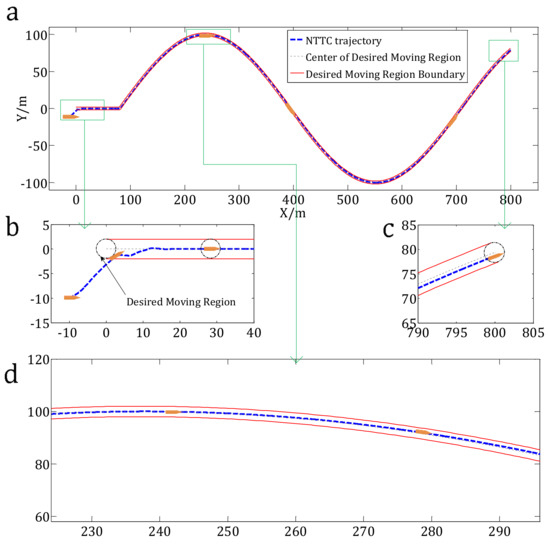
Figure 5.
Results of the NTTC method. (a) Trajectory of the USV using the NTTC method; (b) Zoom view of the results from −10 to 40 m in the X direction; (c) Zoom view of the results from 790 to 805 m in the X direction; (d) Zoom view of the results from 225 to 298 m in the X direction.
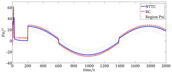
Figure 6.
Yaw angles of the USV under the two control methods.

Figure 7.
Position tracking errors in X direction.
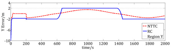
Figure 8.
Position tracking errors in Y direction.
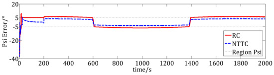
Figure 9.
Yaw tracking errors.
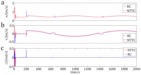
Figure 10.
Velocities of the USV. (a) Surge velocities of the USV using the RC and NTTC method; (b) Sway velocities of the USV using the RC and NTTC method; (c) Yaw velocities of the USV using the RC and NTTC method.
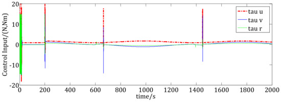
Figure 11.
Control inputs of the USV under the traditional RC method.
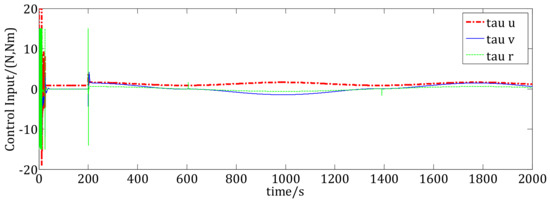
Figure 12.
Control inputs of the USV under the NTTC method.
Figure 4a shows the region tracking results of the RC method. Figure 4b–d show the details of several parts of the tracking results. The red solid lines are the boundaries of the desired moving region. The dashed circle denotes the desired moving region, and the dashed line is the trajectory of the center of the moving-region. The blue dashed line is the trajectory of the USV that is controlled by the RC method.
Figure 5a shows the trajectory tracking results of the NTTC method. Figure 5b–c are used to show the details of several parts of the tracking results. The red solid lines are the boundaries of the desired moving region. The dashed circle denotes the desired moving region, and the dashed line presents the trajectory of the center of the moving-region. The blue dashed line is the trajectory of the USV that is controlled by the NTTC method.
Figure 4 and Figure 5 indicate that the tracking trajectories of the USV fit the desired moving region. However, the USV converges to the boundaries of the desired moving region, as shown in Figure 4. Since the USV’s motion is often influenced by winds, waves or currents, it will move out of the desired region by those disturbances. However, the USV converges into the desired moving region rather than the boundaries of the desired moving region under the proposed NTTC control scheme, which works better than the traditional RC control scheme (Figure 5).
Figure 6 shows the yaw tracking results of the USV. From the figure, the yaw converges into the desired yaw moving region under the NTTC method. However, under the RC method, the USV’s yaw converges to the bounds of the desired yaw moving region.
Figure 7, Figure 8 and Figure 9 show the tracking errors of the USV. In Figure 7, the black dashed lines are the boundaries of the desired region in the X direction, the red dashed line is the tracking error using the RC method, and the blue line shows the tracking error of the NTTC method. We can see that the errors are closed to zero, that is to say, under the RC and the NTTC method, the tracking errors in the direction converge into , which satisfies the desired position region. In Figure 8, the black dashed lines are the boundaries of the desired region in the Y direction, the red dashed line is the tracking error using the NTTC method, and the blue line shows the tracking error of the RC method. We can see that, under the RC method, the position tracking error in the direction converges to the position regional boundaries. However, when there are external disturbances, the error will be easy to move out of the desired region, which is not good for the USV’s control. However, under the NTTC method, the position tracking error converges into the desired region , and it satisfies the desired position region. Figure 9 shows the yaw tracking errors. The yaw error under the NTTC method converges into , which satisfies the desired yaw region. However, the yaw error under the RC method converges to the boundaries of the desired yaw region, and even out of the boundaries at some time points, such as 300 s to 400 s. Hence, the NTTC method is better than the RC method.
Figure 10 shows the velocities of the USV using the RC method and the NTTC method. In Figure 10, Figure 10a shows the velocities using the NTTC method and the RC method, Figure 10b shows the velocities and Figure 10c shows the yaw velocities. We can see that, at t = 200 s, 600 s and 1400 s, there are overshoots for the velocities using the RC method, however, the velocities using the NTTC method are smoother than using the RC method. Figure 11 and Figure 12 are the control inputs during the trajectory tracking. In Figure 11, the control inputs using the RC method are chattering during some time point. However, in Figure 12, the control inputs using the NTTC method are smoother. We can see that the control inputs under the NTTC method change less frequently than those under the RC method.
To further illustrate the advantages of the NTTC method, wave disturbances were added in the next simulations. A linear wave response approximation for wave disturbances is usually preferred by ship control systems engineers, due to its simplicity and applicability [26]. The wave spectrum can be approximated by a second-order system, as shown as follows:
where is the gain constant, is a constant describing the wave intensity, is a damping coefficient and is the dominating wave frequency [26].
In this simulation case, the simulation time is 200 s, and is chosen as 0.5, is chosen as 0.1 and is chosen as 0.8. The other parameters are not changed.
The simulation results are shown in Figure 13, Figure 14, Figure 15, Figure 16, Figure 17 and Figure 18. Figure 13 Figure 14 and Figure 15 show the simulation results using the RC method, and Figure 16, Figure 17 and Figure 18 are the simulation results using the NTTC method.
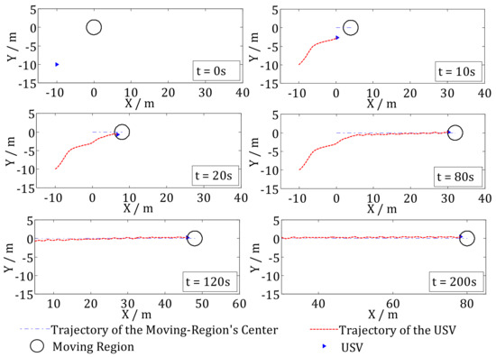
Figure 13.
Trajectory tracking results under the traditional RC method.
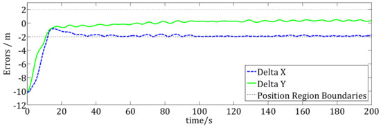
Figure 14.
Position errors of the USV under the traditional RC method.
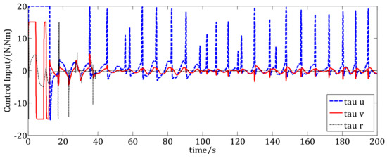
Figure 15.
Control inputs of the USV under the traditional the method.
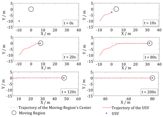
Figure 16.
Trajectory tracking results under the NTTC method.
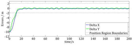
Figure 17.
Position errors of the USV under the NTTC method.
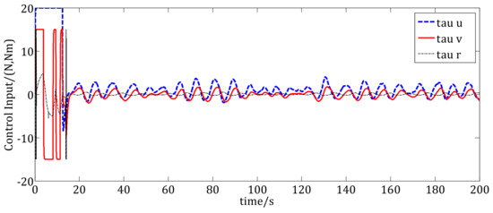
Figure 18.
Control inputs of the USV under the NTTC.
In Figure 13, the desired trajectory of the moving region is a straight line. The USV tracks the moving region using the traditional RC method. The trajectory tracking simulation results at t = 0 s, 10 s, 20 s, 80 s, 120 s, 200 s are also presented in Figure 13. The circle is the desired moving region, the blue dashed line is the trajectory of the desired moving region’s center. The red dashed line is the trajectory of the USV under the RC control method and the blue triangle shows the USV. We can see that because of influenced by the wave disturbances, the trajectory of the USV is chattering. After about t = 20 s, the USV converges to the boundary of the desired moving region, which is the same as the results in Figure 4. However, Figure 14 shows that the position error in the X direction converges to the boundary of the desired error region. Under wave disturbances, the USV will move in and out of the desired moving-region frequently, which will cause frequently control inputs as shown in Figure 15. Figure 15 is the results of control inputs of the USV using the RC control method. We can see that the control inputs chattering frequently under wave disturbances, which is bad for the USV’s propellers.
Nevertheless, in Figure 16, the USV converges into the moving region other than the boundary of the desired moving region under the NTTC method. To be consistent with the simulation in Figure 13, the trajectory tracking simulation results at t = 0 s, 10 s, 20 s, 80 s, 120 s, and 200 s are also shown in Figure 16. The circle is the desired moving region, the blue dashed line is the trajectory of the desired moving region’s center. The red dashed line is the trajectory of the USV under NTTC control method and the blue triangle shows the USV. We can see that the trajectory is influenced by the wave disturbances, so it isn’t a straight line. After about t = 20 s, the USV converges into the desired moving region, which is the same as the results in Figure 5. Figure 17 show the position errors using NTTC method. The difference with Figure 14 is that the position error in X direction converges into the error region other than the boundary of the error region. Figure 18 is the results of control inputs of the USV using NTTC method, we can see that the NTTC method gives more smooth control inputs for the USV when there are disturbances.
To compare the control inputs of the two methods, we use the Root-Mean-Square (RMS) value of the control inputs to measure their performance. The comparisons are shown in Table 2. The RMSs of control inputs using NTTC method are smaller than that using the RC method.
Table 2.
Control input comparisons of RC and NTTC method.
The comparison of the simulation results of Figure 15 and Figure 18 indicates that the NTTC method works better under disturbances than the RC method. Moreover, the control inputs under the NTTC method change less frequently than those under the RC method, which is good for the actuating mechanisms of the USV and saves energy.
5. Conclusions
In this study, an adaptive trajectory tracking control scheme called NTTC is proposed for non-strict trajectory tracking of a fully actuated USV. The controller is designed using a regression matrix, RC scheme, and a switching gain controller term, such that the USV converges into the desired moving region trajectory and tracks the desired position within the region boundary with desired orientation. The closed-loop stability of the system is proved by the Lyapunov stability theorem. The simulation results demonstrate the effectiveness of the proposed control scheme and shows that under the proposed NTTC method, the USV can track straight-line region trajectory and curve region trajectory well. The simulation results also show that the proposed NTTC method performs better than the traditional RC method. The method allows the trajectory of the USV to converge into the desired moving region rather than the boundary of the moving region, and reduces the system’s chattering at the same time. This condition is good for the actuating mechanisms of the USV and is energy efficient. However, the proposed method is only used for a fully actuated USV in this study. Further work should consider using underactuated USVs.
Acknowledgments
The authors wish to thank the State Key Laboratory of Ocean Engineering, Laboratory of Intelligent Equipment and System at Sea of Shanghai Jiao Tong University, for their support of this study.
Author Contributions
Jian Wang, Jing-yang Liu and Hong Yi conceived the main concept and contributed the analysis. Jian Wang wrote the paper, and Nai-long Wu performed a spell check. All authors contributed in writing the final manuscript.
Conflicts of Interest
The authors declare no conflict of interest.
References
- Liu, Z.X.; Zhang, Y.M.; Yu, X.; Yuan, C. Unmanned surface vehicles: An overview of developments and challenges. Annu. Rev. Control 2016, 41, 71–93. [Google Scholar] [CrossRef]
- Pettersen, K.Y.; Nijmeijer, H. Underactuated ship tracking control: Theory and experiments. Int. J. Control 2001, 74, 1435–1446. [Google Scholar] [CrossRef]
- Encarnacao, P.; Pascoal, A. Combined Trajectory Tracking and Path Following: An Application to the Coordinated Control of Autonomous Marine Craft. In Proceedings of the 40th IEEE Conference on Decision and Control, Orlando, FL, USA, 4–7 December 2001. [Google Scholar]
- Cheng, J.; Yi, J.; Zhao, D. Design of a sliding mode controller for trajectory tracking problem of marine vessels. IET Control Theory Appl. 2007, 1, 233–237. [Google Scholar]
- Fahimi, F.; Van Kleeck, C. Alternative trajectory-tracking control approach for marine surface vessels with experimental verification. Robotica 2013, 31, 25–33. [Google Scholar] [CrossRef]
- Yang, Y.; Du, J.; Liu, H.; Guo, C.; Abraham, A. A trajectory tracking robust controller of surface vessels with disturbance uncertainties. IEEE Trans. Control Syst. Technol. 2014, 22, 1511–1518. [Google Scholar] [CrossRef]
- Soltan, R.A.; Ashrafiuon, H.; Muske, K.R. State-dependent Trajectory Planning and Tracking Control of Unmanned Surface Vessels. In Proceedings of the American Control Conference, St. Louis, MO, USA, 10–12 June 2009. [Google Scholar]
- Zhang, L.J.; Jia, H.M.; Xue, Q. NNFFC-adaptive output feedback trajectory tracking control for a surface ship at high speed. Ocean Eng. 2011, 38, 1430–1438. [Google Scholar] [CrossRef]
- Wang, C.S.; Zhang, H.; You, Y. USV Trajectory Tracking Control System Based on ADRC. In Proceedings of the Chinese Automation Congress (CAC), Jinan, China, 20–22 October 2017. [Google Scholar]
- Fu, M.Y.; Zhou, L.; Xu, Y.J. Bio-inspired Trajectory Tracking Algorithm Based on SFLOS for USV. In Proceedings of the 36th Chinese Control Conference, Dalian, China, 26–28 July 2017. [Google Scholar]
- Gao, Y.; Wang, N.; Zhang, W.D. Disturbance Observer Based Finite-Time Trajectory Tracking Control of Unmanned Surface Vehicles with Unknown Dead-Zones. In Proceedings of the 2017 32nd Youth Academic Annual Conference of Chinese Association of Automation (YAC), Hefei, China, 19–21 May 2017. [Google Scholar]
- Wang, N.; Gao, Y.; Lv, S.L.; Er, M.J. Integral sliding mode based finite-time trajectory tracking control of unmanned surface vehicles with input saturations. Indian J. Geo-Mar. Sci. 2017, 46, 2493–2501. [Google Scholar]
- Wang, N.; Gao, Y.; Sun, Z.; Zheng, Z.J. Nussbaum-based adaptive fuzzy tracking control of unmanned surface vehicles with fully unknown dynamics and complex input nonlinearities. Int. J. Fuzzy Syst. 2018, 20, 259–268. [Google Scholar] [CrossRef]
- Qu, Y.H.; Xiao, B.; Fu, Z.Z.; Yuan, D.L. Trajectory exponential tracking control of unmanned surface ships with external disturbance and system uncertainties. ISA Trans. 2018. [Google Scholar] [CrossRef]
- Dong, Z.P.; Wan, L.; Li, Y.M.; Liu, T.; Zhang, G.C. Trajectory tracking control of underactuated USV based on modified backstepping approach. Int. J. Nav. Archit. Ocean Eng. 2015, 7, 817–832. [Google Scholar] [CrossRef]
- Liu, C.; Zou, Z.J.; Yin, J.C. Trajectory tracking of underactuated surface vessels based on neural network and hierarchical sliding mode. J. Mar. Sci. Technol. 2015, 20, 322–330. [Google Scholar] [CrossRef]
- Chen, X.T.; Tan, W.W. Tracking control of surface vessels via fault-tolerant adaptive backstepping interval type-2 fuzzy control. Ocean Eng. 2013, 70, 97–109. [Google Scholar] [CrossRef]
- Cheah, C.C.; Wang, D.Q.; Sun, Y.C. Region-reaching control of robots. IEEE Trans. Robot. 2007, 23, 1260–1264. [Google Scholar] [CrossRef]
- Cheah, C.C.; Sun, Y.C. Adaptive Region Control For Autonomous Underwater Vehicles. In Proceedings of the MTTS/IEEE TECHNO-OCEAN’04, Kobe, Japan, 9–12 Novemeber 2004. [Google Scholar]
- Sun, Y.C.; Cheah, C.C. Region-reaching control for underwater vehicle with onboard manipulator. IET Control Theory Appl. 2008, 2, 819–828. [Google Scholar] [CrossRef]
- Haghighi, R.; Cheah, C.C. Multi-group coordination control for robot swarms. Automatica 2012, 48, 2526–2534. [Google Scholar] [CrossRef]
- Li, X.; Hou, S.P.; Cheah, C.C. Adaptive Region Tracking Control for Autonomous Underwater Vehicle. In Proceedings of the 11th International Conference on Control Automation Robotics & Vision (ICARCV), Singapore, 7–10 December 2010. [Google Scholar]
- Ismail, Z.H.; Matthew, W.D. Nonlinear optimal control scheme for an underwater vehicle with regional function formulation. J. Appl. Math. 2013, 2013, 732738. [Google Scholar] [CrossRef]
- Ismail, Z.H.; Matthew, W.D. A region boundary-based control scheme for an autonomous underwater vehicle. Ocean Eng. 2011, 38, 2270–2280. [Google Scholar] [CrossRef]
- Mukherjee, K.; Kar, I.N.; Bhatt, R.K.P. Region tracking based control of an autonomous underwater vehicle with input delay. Ocean Eng. 2015, 99, 107–114. [Google Scholar] [CrossRef]
- Fossen, T.I. Handboof of Marine Craft Hydrodynamics and Motion Control, 1st ed.; John Wiley & Sons Ltd.: Chichester, UK, 2011. [Google Scholar]
- Skjetne, R.; Smogeli, Ø.N.; Fossen, T.I. A nonlinear ship manoeuvering model: Identification and adaptive control with experiments for a model ship. Model. Identif. Control 2004, 25, 3–27. [Google Scholar] [CrossRef]
- Skjetne, R.; Fossen, T.I.; Petar, V.K. Adaptive maneuvering, with experiments, for a model ship in a marine control laboratory. Automatica 2005, 41, 289–298. [Google Scholar] [CrossRef]
© 2018 by the authors. Licensee MDPI, Basel, Switzerland. This article is an open access article distributed under the terms and conditions of the Creative Commons Attribution (CC BY) license (http://creativecommons.org/licenses/by/4.0/).