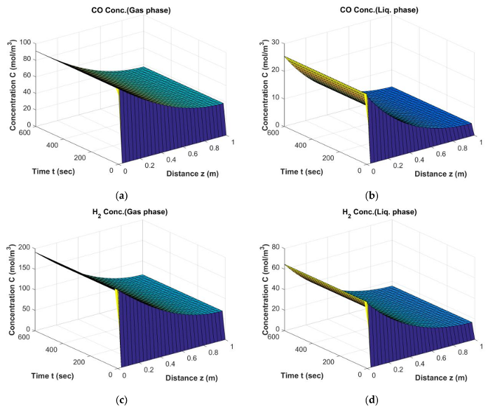
Figure 1.
Results of Fischer–Tropsch (FT) Simulation; The behavior of CO, H2 in gas phase (a,c) and liquid phase (b,d) from start-up to steady state conditions (Dt = 0.1 m, H = 2.5 m, = 0.34, Ug,in = 0.17 m/s).
Figure 1.
Results of Fischer–Tropsch (FT) Simulation; The behavior of CO, H2 in gas phase (a,c) and liquid phase (b,d) from start-up to steady state conditions (Dt = 0.1 m, H = 2.5 m, = 0.34, Ug,in = 0.17 m/s).
Figure 2.
Results of FT Simulation; The behavior of H2O and CO2 in gas phase (a,c) and liquid phase (b,d) from start-up to steady state conditions (Dt = 0.1 m, H = 2.5 m, = 0.34, Ug,in = 0.17 m/s).
Figure 2.
Results of FT Simulation; The behavior of H2O and CO2 in gas phase (a,c) and liquid phase (b,d) from start-up to steady state conditions (Dt = 0.1 m, H = 2.5 m, = 0.34, Ug,in = 0.17 m/s).
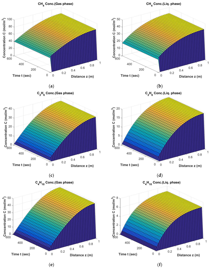
Figure 3.
Results of FT Simulation; The behavior of CH4, C2H6 and C4H10 in gas phase (a,c,e) and liquid phase (b,d,f) from start-up to steady state conditions (Dt = 0.1 m, H = 2.5 m, = 0.34, Ug,in = 0.17 m/s).
Figure 3.
Results of FT Simulation; The behavior of CH4, C2H6 and C4H10 in gas phase (a,c,e) and liquid phase (b,d,f) from start-up to steady state conditions (Dt = 0.1 m, H = 2.5 m, = 0.34, Ug,in = 0.17 m/s).
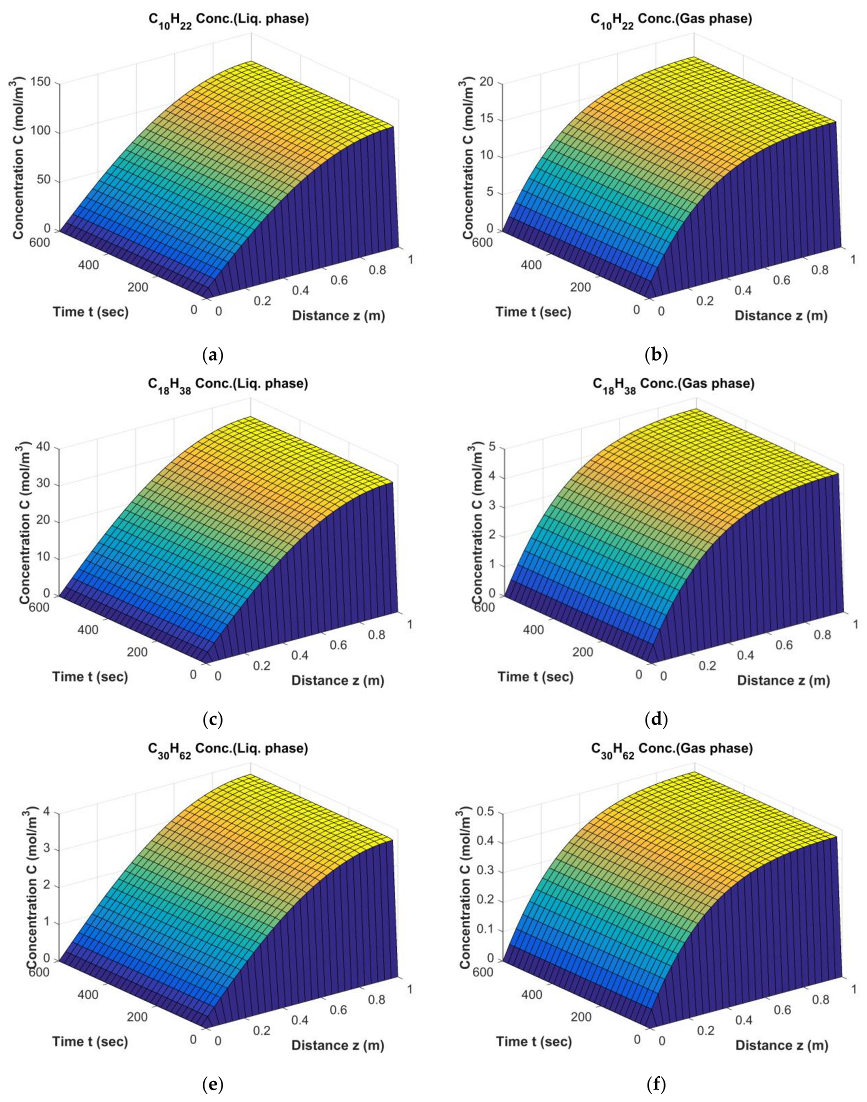
Figure 4.
Results of FT simulation; The behavior of C10H22, C18H38 and C30H62 in liquid phase (a,c,e) and gas phase (b,d,f) from start-up to steady state conditions (Dt = 0.1 m, H = 2.5 m, = 0.34, Ug,in = 0.17 m/s).
Figure 4.
Results of FT simulation; The behavior of C10H22, C18H38 and C30H62 in liquid phase (a,c,e) and gas phase (b,d,f) from start-up to steady state conditions (Dt = 0.1 m, H = 2.5 m, = 0.34, Ug,in = 0.17 m/s).
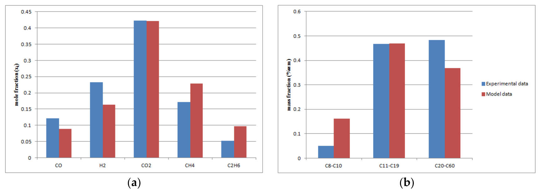
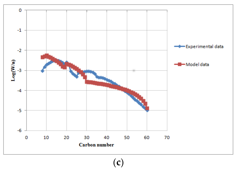
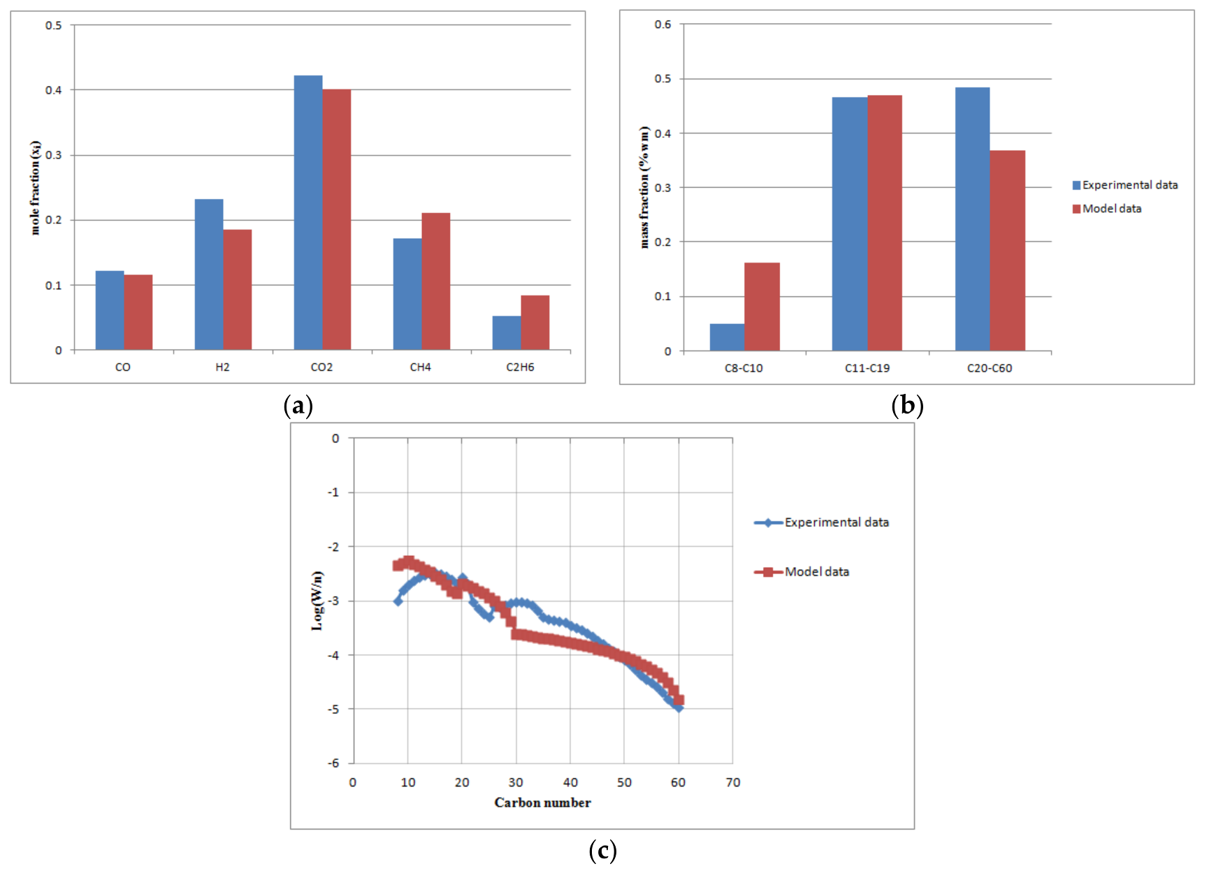
Figure 5.
The comparison of the predicted model with experimental data at base load conditions (volumetric gas flow rate 5 m3/h, T = 503 K, = 0.34, P = 20 bar): (a) off-gas molar fractions; (b) FT products (naphta, diesel, wax); (c) ASF distribution.
Figure 5.
The comparison of the predicted model with experimental data at base load conditions (volumetric gas flow rate 5 m3/h, T = 503 K, = 0.34, P = 20 bar): (a) off-gas molar fractions; (b) FT products (naphta, diesel, wax); (c) ASF distribution.
Figure 6.
The comparison of the predicted model with experimental data at change load conditions (volumetric gas flow rate 3.5 m3/h, T = 503 K, = 0.34, P = 20 bar): (a) off-gas molar fractions; (b) FT products (naphta, diesel, wax); (c) ASF distribution.
Figure 6.
The comparison of the predicted model with experimental data at change load conditions (volumetric gas flow rate 3.5 m3/h, T = 503 K, = 0.34, P = 20 bar): (a) off-gas molar fractions; (b) FT products (naphta, diesel, wax); (c) ASF distribution.
Figure 7.
The comparison of the predicted model with experimental data at change load conditions (volumetric gas flow rate 7.5 m3/h, T = 503 K, = 0.34, P = 20 bar): (a) off-gas molar fractions; (b) FT products (naphtha, diesel, wax); (c) ASF distribution.
Figure 7.
The comparison of the predicted model with experimental data at change load conditions (volumetric gas flow rate 7.5 m3/h, T = 503 K, = 0.34, P = 20 bar): (a) off-gas molar fractions; (b) FT products (naphtha, diesel, wax); (c) ASF distribution.
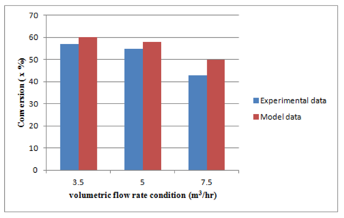
Figure 8.
CO Conversion at base and change load condition based on experimental and model data.
Figure 8.
CO Conversion at base and change load condition based on experimental and model data.
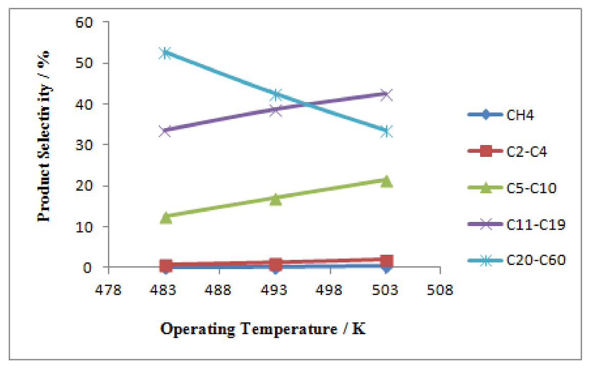
Figure 9.
Influence of operating temperature on product selectivity; Dt = 0.1 m, H = 2.5 m, Vf = 3.5 m3/h, P = 20 bar, = 0.34.
Figure 9.
Influence of operating temperature on product selectivity; Dt = 0.1 m, H = 2.5 m, Vf = 3.5 m3/h, P = 20 bar, = 0.34.
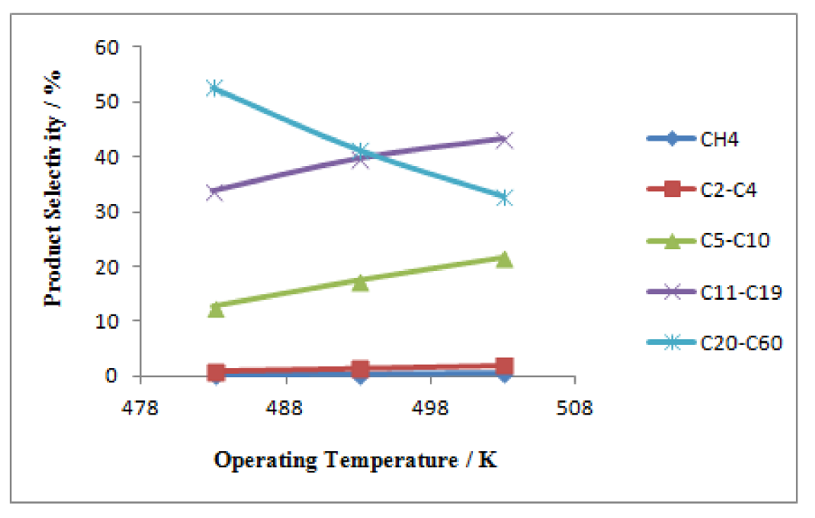
Figure 10.
Influence of operating temperature on product selectivity; Dt = 0.1 m, H = 2.5 m, Vf = 5 m3/h, P = 20 bar, = 0.34.
Figure 10.
Influence of operating temperature on product selectivity; Dt = 0.1 m, H = 2.5 m, Vf = 5 m3/h, P = 20 bar, = 0.34.
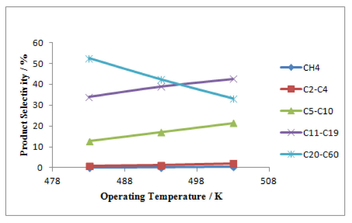
Figure 11.
Influence of operating temperature on product selectivity; Dt =0.1 m, H = 2.5 m, Vf = 7.5 m3/h, P = 20 bar, = 0.34.
Figure 11.
Influence of operating temperature on product selectivity; Dt =0.1 m, H = 2.5 m, Vf = 7.5 m3/h, P = 20 bar, = 0.34.
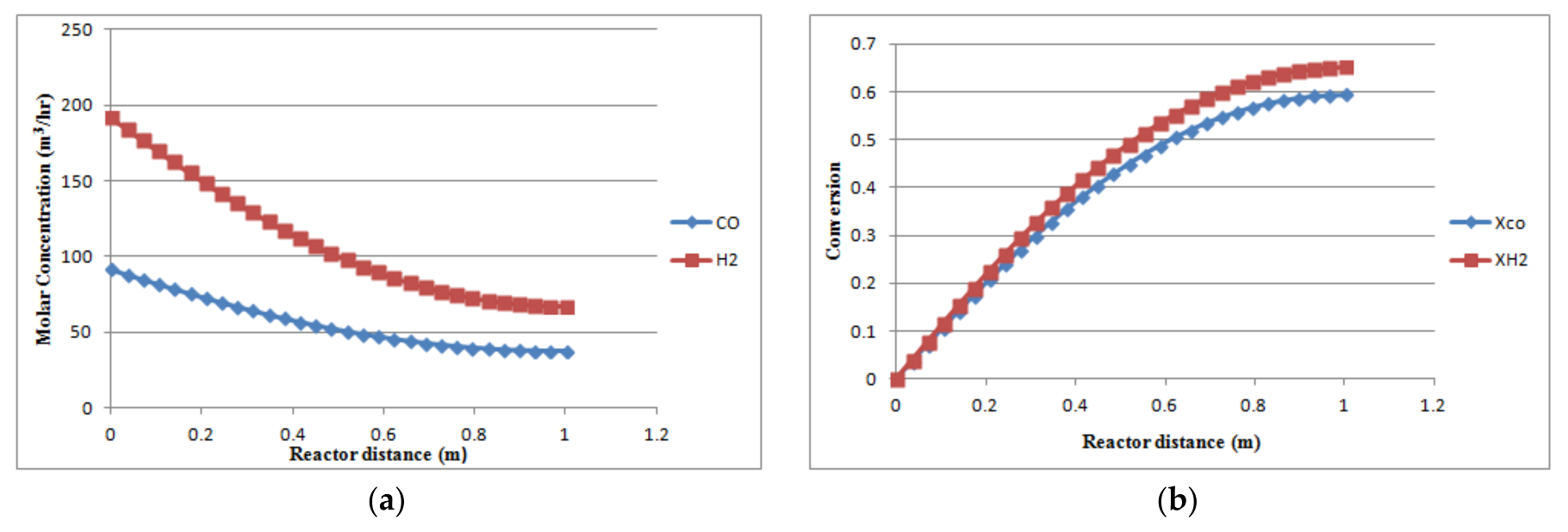
Figure 12.
The syngas variation on the reactor inside, (a) Molar concentration of CO and H2; (b) CO and H2 conversion.
Figure 12.
The syngas variation on the reactor inside, (a) Molar concentration of CO and H2; (b) CO and H2 conversion.
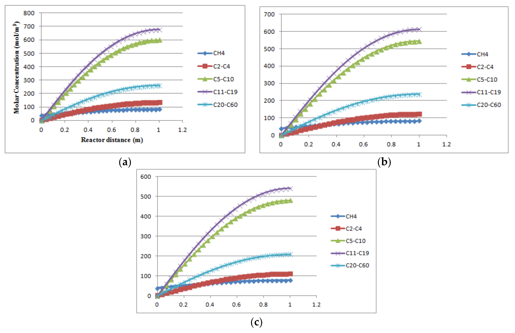
Figure 13.
The molar concentration of the FT products along the reactor bed at three load conditions: (a) T = 503 K, P = 20 bar, Vf = 3.5 m3/h; (b) T = 503 K, P = 20 bar, Vf =5 m3/h; (c) T = 503 K, P = 20 bar, Vf = 7.5 m3/h.
Figure 13.
The molar concentration of the FT products along the reactor bed at three load conditions: (a) T = 503 K, P = 20 bar, Vf = 3.5 m3/h; (b) T = 503 K, P = 20 bar, Vf =5 m3/h; (c) T = 503 K, P = 20 bar, Vf = 7.5 m3/h.
Figure 14.
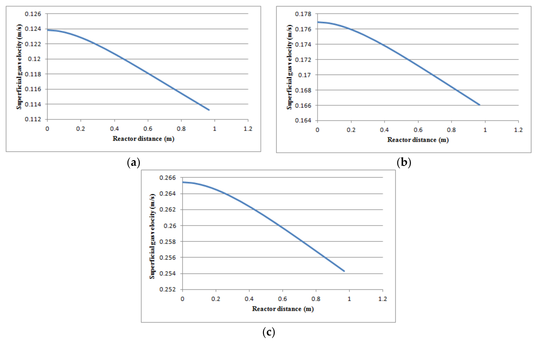
Reduction of superficial gas velocity as a function of reactor height at three different operating load conditions: (a) T = 503 K, P = 20 bar, Vf = 3.5 m3/h; (b) T = 503 K, P = 20 bar, Vf = 5 m3/h; (c) T = 503 K, P = 20 bar, Vf = 7.5 m3/h.
Figure 14.
Reduction of superficial gas velocity as a function of reactor height at three different operating load conditions: (a) T = 503 K, P = 20 bar, Vf = 3.5 m3/h; (b) T = 503 K, P = 20 bar, Vf = 5 m3/h; (c) T = 503 K, P = 20 bar, Vf = 7.5 m3/h.
Table 1.
Kinetic Characteristics of Fischer–Tropsch Slurry Bubble Column reactor (FT-SBCR): reaction parameters, product distribution.
Table 1.
Kinetic Characteristics of Fischer–Tropsch Slurry Bubble Column reactor (FT-SBCR): reaction parameters, product distribution.
| Reaction Characteristics | Relations | Constants, Parameters and Paraffin Reaction Form |
|---|
| Reaction Kinetics | | a = 1.59064 × 10⁻¹² |
| b = 7.99389 × 10⁻⁶ |
| Chain grow probability factor (Song et al.) | | A = 0.2332 | B = 0.633 |
| |
| Anderson Sculz-Flory distribution of products. | | |
| Rate of paraffin formation based on ASF distribution. | | |
Table 2.
Operating conditions and liquid properties of lab-scale Fischer–Tropsch Slurry Bubble Column.
Table 2.
Operating conditions and liquid properties of lab-scale Fischer–Tropsch Slurry Bubble Column.
| Operating Condition |
| Reactor Temperature | 503 K |
| Reactor Pressure | 20 bar |
| H2/CO | 2 |
| Reactor diameter | 0.1 m |
| Reactor height | 2.5 m |
| Volumetric Flow Rate (loads) | 3.5, 5, 7.5 m3/h |
| Liquid Phase Properties |
| Liquid Density | 715 kg/m3 |
| Surface tension | 0.023 N/m |
| Liquid Viscosity | 3 × 10⁻³ Pa.s |
Table 3.
Initial and boundary conditions for the slurry reactor model.
Table 3.
Initial and boundary conditions for the slurry reactor model.
| Initial Condition (t = 0) | Reactor Inlet (z = 0) | Reactor Outlet (z = H) |
|---|
| Cgi = Cgi,in | Cgi = Cgi,in
| |
| Cli = Cgi,in/Ai | | |
| Ui = Ug,in | Ugi = Ug,in | |

 ,
, 


