Article

Growth Identification of Aspergillus flavus and Aspergillus parasiticus by Visible/Near-Infrared Hyperspectral Imaging

1
College of Engineering, China Agricultural University, Beijing 100083, China
2
Crop Genetics and Breeding Research Unit, USDA-ARS, 2747 Davis Road, Tifton, GA 31793, USA
3
College of Food Science & Nutritional Engineering, China Agricultural University, Beijing 100083, China
4
College of Information Engineering, Tarim University, Alar 843300, China
5
Multidisciplinary Initiative Center, Institute of High Energy Physics, Chinese Academy of Sciences, Beijing 100049, China
*
Authors to whom correspondence should be addressed.
These authors contributed equally to this work and should be considered co-first authors
Appl. Sci. 2018, 8(4), 513; https://doi.org/10.3390/app8040513
Submission received: 8 February 2018 / Revised: 28 February 2018 / Accepted: 12 March 2018 / Published: 28 March 2018
(This article belongs to the Special Issue Hyperspectral Chemical Imaging for Food Authentication)

Abstract

:
Visible/near-infrared (Vis/NIR) hyperspectral imaging (400–1000 nm) was applied to identify the growth process of Aspergillus flavus and Aspergillus parasiticus. The hyperspectral images of the two fungi that were growing on rose bengal medium were recorded daily for 6 days. A band ratio using two bands at 446 nm and 460 nm separated A. flavus and A. parasiticus on day 1 from other days. Image at band of 520 nm classified A. parasiticus on day 6. Principle component analysis (PCA) was performed on the cleaned hyperspectral images. The score plot of the second to sixth principal components (PC2 to PC6) gave a rough clustering of fungi in the same incubation time. However, in the plot, A. flavus on day 3 and day 4 and A. parasiticus on day 2 and day 3 overlapped. The average spectra of each fungus in each growth day were extracted, then PCA and support vector machine (SVM) classifier were applied to the full spectral range. SVM models built by PC2 to PC6 could identify fungal growth days with accuracies of 92.59% and 100% for A. flavus and A. parasiticus individually. In order to simplify the prediction models, competitive adaptive reweighted sampling (CARS) was employed to choose optimal wavelengths. As a result, nine (402, 442, 487, 502, 524, 553, 646, 671, 760 nm) and seven (461, 538, 542, 742, 753, 756, 919 nm) wavelengths were selected for A. flavus and A. parasiticus, respectively. New optimal wavelengths SVM models were built, and the identification accuracies were 83.33% and 98.15% for A. flavus and A. parasiticus, respectively. Finally, the visualized prediction images for A. flavus and A. parasiticus in different growth days were made by applying the optimal wavelength’s SVM models on every pixel of the hyperspectral image.

Graphical Abstract

1. Introduction

Aspergillus flavus and the closely related subspecies Aspergillus parasiticus have long been recognized as major contaminants of organic and nonorganic items [1]. They can contaminate a wide range of agricultural products, lead to sensorial, nutritional changes like pigmentation, discoloration, and rotting [2]. Moreover, they can produce aflatoxin under appropriate conditions [3]. If they infects food and feeds (such as maize, rice, peanuts, etc.), the aflatoxin may cause mycotoxicoses in animals and humans [4]. Although the presence of Aspergillus spp. does not necessarily indicate the occurrence of aflatoxin, it presents the possibility of the appearance of aflatoxin [5]. Accordingly, it is important and necessary to early detect and identify toxic fungi.
Traditional culturing methods are the gold standard for microorganism detection. Identification of the fungal growth is mainly based on the macroscopic and microscopic biological characteristics of the fungus. In specific condition, total viable count, biomass, and metabolite production concentrations were utilized to describe fungal growth [6,7,8,9], while fungal DNA extraction, polymerase chain reaction (PCR), and agarose gel electrophoresis were investigated for accurate fungal detection [10]. However, traditional culturing and biological analysis were time consuming and laborious; in particular, they required additional chemicals and even produced toxic by-products. Thus, non-destructive optical methods for the detection of microorganisms are becoming increasingly important [11].
Hyperspectral imaging (HSI) is an optical imaging technique that combines conventional imaging and vibrational spectroscopy and provides both spatial and spectral information simultaneously [12,13]. The spatial and spectral information are contained in a 3D hyperspectral image dataset, which contains two spatial dimensions and one spectral dimension [14]. Thus in the hyperspectral image, the spectrum of each pixel and image of each wavelength band can be analysed synergistically.
In recent years, hyperspectral imaging was widely used to detect fungal contamination on cereals. Del Fiore et al. used visible-near infrared (Vis/NIR) hyperspectral imaging (400–1000 nm) to early detect maize kernels inoculated with different toxigenic fungi. Results indicated that the method could identify A. flavus and A. niger contaminants on the maize, starting at 48 h from inoculation [15]. Kheiralipour et al. used near-infrared hyperspectral imaging (800–2600 nm)-determined pistachio kernels infected by toxigenic and atoxigenic A. flavus (KK11 and R5) and classified the kernel infection by those two fungi at the last fungal growing stage [16]. Zhao et al. detected the contamination level of maize kernels inoculated with A. parasiticus by using hyperspectral images with a spectral range of 1000–2500 nm. The studies showed that hyperspectral imaging has become a promising non-destructive technique for detecting the fungal contamination levels and fungal species on cereals [17].
However, fungal development on food product is complex; thus, to detect fungi in its early stage, it is necessary to investigate microorganisms in a controlled manner and environment first. For example, there have been some publications that have reported the use of hyperspectral imaging to detect fungi plated on the culture medium. Yao et al. identified five types of toxigenic fungi on day 5 of growth using a hyperspectral image, and all five fungi can be easily separated by only three wavelength bands (743, 458 and 541 nm) [18]. Jin et al. classified toxigenic and atoxigenic A. flavus using a hyperspectral image under UV light and halogen light source [19]. This research focused on discriminating the species of the fungi only at one fixed mature stage of growth. In recent years, there have also been some studies that have analyzed the development of fungi. Williams et al. constructed growth curves of three Fusarium spp. and visualized the radial growth zones within the colonies [20,21]. Dégardin et al. measured the growth of the A. flavus colony using the Vis/NIR HSI technique. Results showed that the reflectance of the colony surface in different growth periods was significantly different in some wavelength regions [22]. Sun et al. also pointed out that the fungal color, shape, and chemical composition would change with the growth of fungi, which could affect the spectral absorption [7]. They also built fungal growth simulation models based on parameters of the hyperspectral image. This research all showed the potential of hyperspectral imaging to be expanded to detect fungal characteristics grown on agar media. Nevertheless, there were still limited studies for the detection of specific growth characteristics of A. flavus and A. parasiticus, the main aflatoxin-producing fungi on media, using the HSI technique.
The objective of the present work was to investigate the potential of hyperspectral imaging to identify optical features of the two aflatoxin producing fungi, A. flavus and A. parasiticus, which are inoculated on same rose bengal media under uniform environmental conditions for different days.

2. Materials and Methods

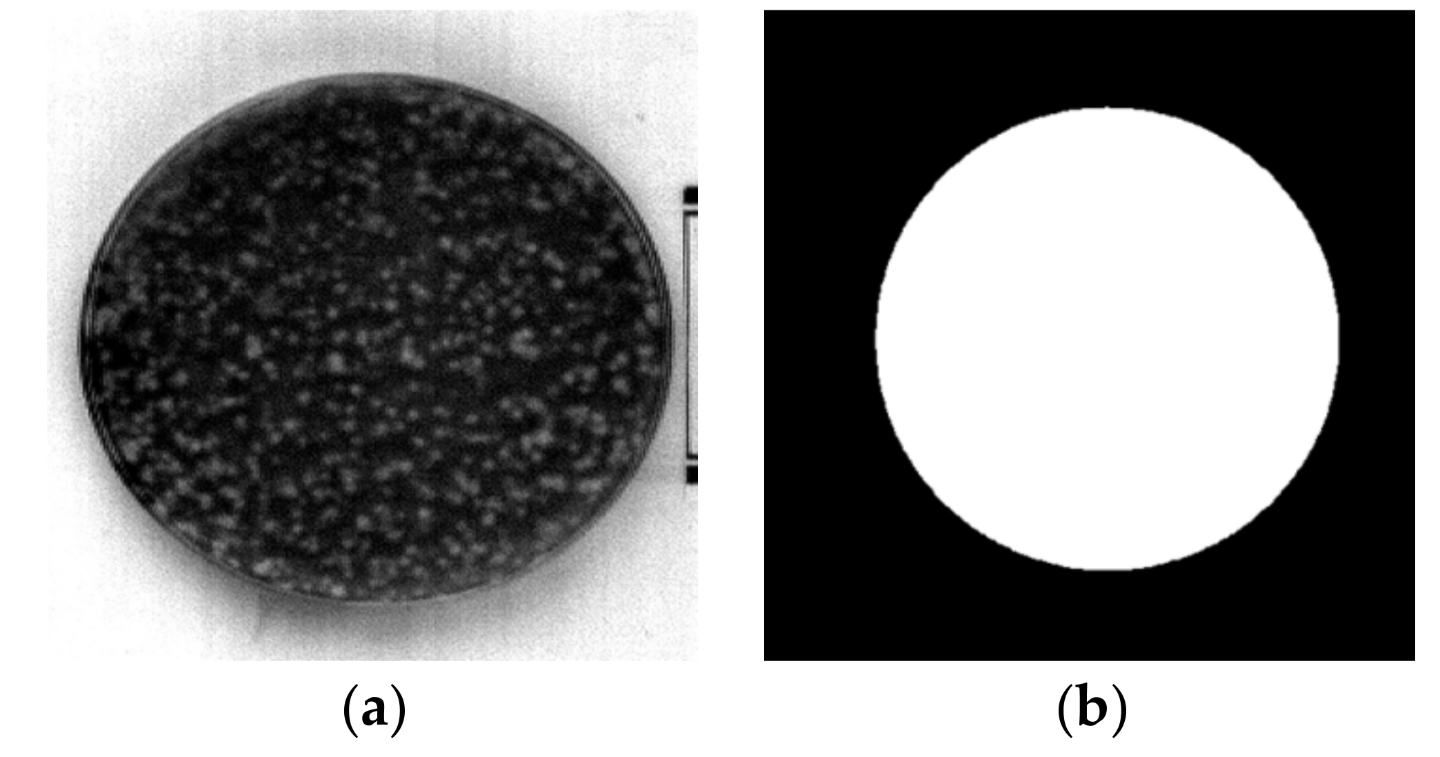
2.1. Sample Preparation

In this study, Aspergillus flavus (strain number: CGMCC 3.6304) and Aspergillus parasiticus (strain number: CGMCC 3.6155) were obtained from China General Microbiological Culture Collection Center (CGMCC, Beijing, China) and grown on potato dextrose agar (PDA) media at 30 °C. After 7 days, conidia were harvested by a sterile inoculation loop and suspend in sterile 0.9% saline. Thereafter, the conidial suspensions were adjusted to 106 spores mL−1 using a haemocytometer (Qiujing, Shanghai, China). Each kind of fungus was inoculated by mixing rose bengal media with 1 mL of respective fungal spore suspension in Petri dishes. The inoculation was performed for 6 days with regular intervals of 24 h. The inoculation in each day was repeated on three different plates, resulting in three replicates. Hence, there were totally 18 Petri dishes (6 days × 3 replicates) for A. flavus and 18 Petri dishes for A. parasiticus. All plates were incubated at 30 °C in a constant and humid incubator.

2.2. Image Acquisition and Calibration

The Visible/near-infrared (Vis/NIR) hyperspectral imaging system used for the experiments consisted of an Offner structured spectrometer (N Series, Headwall Photonics, Bolton, MA, USA), an EMCCD detector (Andor, Luca-R EMCCD, Belfast, United Kingdom), a variable-focal-length lens (Schneider, XENOPLAN, Bad Kreuznach, Germany), a motorized stage (WN500TA1000H, Beijing, China), two 500 W Tungsten-Halogen lamps positioned at approximately 45° angles and 35 cm above and lateral to the samples (Photoflex, Watsonville, CA, USA), and a computer with the image acquisition software. The wavelength range of this system was from 350 to 1000 nm with an average wavelength gap of 3.7 nm; the line-scan width contained 1008 pixels, and the pixel resolution of the system was 0.226 × 0.226 mm.
The hyperspectral images were taken in a dark room. The distance of the camera from the target was 40 cm. Exposure time was set as 32 ms, and the speed of the motorized stage was 1.2 cm/s. Prior to imaging, a white reflectance image (W) was taken for image calibration by acquiring the spectral image of a Spectralon® reflectance panel with 100% reflectance values (SRT-75e050, Labsphere, North Sutton, NH, USA), and the dark reference image (B) was obtained by recording the spectral image when the camera lens was completely covered [23]. During imaging, the Petri dish with its lid removed was placed on a white Teflon® (Polytetrafluoroethylene) plate, and then the hyperspectral images were acquired by moving the samples pass by the lens in front of the hyperspectral image camera via the motorized stage. The acquired hyperspectral images (I) were calibrated by the following calibration model:
R = I B W B × 100 %

2.3. Data Analysis Method

2.3.1. Explanatory Method

Images at specific bands, as well as images of specific principal components (PC) score image, were first used to visually evaluate the difference of fungi in different incubation time. In this study, principal component analysis (PCA) was applied on both the hyperspectral image preprocessing and the data analysis. It decomposed the spectral data into several principal components, which were orthogonal to each other and could keep maximum variation of the data points (pixels in case of hyperspectral data) in the original spectral space [24]. In particular, the loading consisted of coefficients that multiplied each variable, which can be used to identify variables that are highly correlated with each PC [25], while the scores of PCA represent the weighted sums of the original variables without significant loss of useful information. PC score images can be got by multiplying image in each band and their loadings matrix [26]. Score vectors can also be used to make scatter plots called PCA score plots, which can give an indication of clustering of groups comprised of similar pixels.

2.3.2. Model Development Method

Average spectra of each fungus in each Petri dish were extracted. The mean reflectance spectra of each regions of interest (ROI) were then extracted and used for training classifiers. PCA and support vector machine (SVM) classifier were applied on the average spectra of full wavelength range to classify fungi in different incubation. Furthermore, optimal wavelengths were selected by competitive adaptive reweighted sampling (CARS) method, and the spectra at those wavelengths were used to build a simplified SVM classification model.
CARS method is used to select an optimal combination of wavelengths with large absolute coefficients in the full spectrum coupled with PLS regression [27]. The absolute values of regression coefficients of PLS model are used as an index when evaluating the importance of each wavelength. N subsets of wavelengths are selected from N Monte Carlo (MC) sampling runs in an iterative and competitive manner. In each sampling run, some samples are first randomly chosen in a fixed ratio to build a calibration model. Then, exponentially decreasing function (EDF), competitive wavelength reduction by adaptive reweighted sampling (ARS), and root mean square error of cross validation (RMSECV) were adopted to select the key variables subset [28,29]. The procedure of CARS was performed in the Matlab 2013b (MathWorks, Natick, MA, USA).
SVM can create a hyperplane that can make the largest classification interval between each class of samples in the higher dimension feature space [30]. Since it was widely used in classification problems, it was utilized to identify fungi at different incubation times and discriminate among fungi species in this study.

3. Result and Discussion

3.1. Hyperspectral Image Preprocessing

Firstly, in order to remove the background region, all the corrected images were then spatially cropped down to 451(W) × 451(H) (Figure 1a). Additionally, only 141 spectral bands ranging from 400 to 920 nm were reserved, because the wavelengths 350–498 nm and 923–1000 nm mainly contributed to noise. Median filter (kernel size 5) was then applied to image at each spectral band to reduce pixel random noise. Moreover, in order to suppress the unwanted background outside of each Petri dish and the shallow at the edge of the dish, all the hyperspectral images were masked by binary plate masks (Figure 1b), which were little smaller than those of the Petri dishes. The masks, i.e., the selection of the ROI area, were created manually by ROI selecting tool in the ENVI software (Exelis Visual Information Solutions, Boulder, CO, USA). In order to apply same algorithms on different images synchronously, pixel-based mosaic for each type of fungi was constructed. Two mosaics were composed of A. flavus and A. parasiticus incubated from 1 to 6 days, respectively. PCA and inverse PCA were conducted to obtain the denoised hyperspectral image data. The first 6 PCs contained the majority of information in the hyperspectral data cube and very little noise. Thus, the first 6 PCs were used in the inverse PCA. The cleaned images were used for subsequent spectral extraction and multivariate classification. Pixel and spectral approach methods were used to find characteristics of fungi growth and distinguish different fungi.

3.2. Identification of Fungal Growth Days by Band Math

In both cases, for A. flavus and A. parasiticus, mycelia started to appear clearly on day 2, which were smooth and white, while conidia on A. parasiticus appeared earlier than A. flavus. On day 4, chartreuse conidia of A. parasiticus emerged. Additionally, when the conidia increased in number and matured, they became darker in color. For A. flavus, a few conidia formed on day 5, and their conidia were not as obvious as those of A. parasiticus. In order to further discriminate fungi inoculated for different days, average spectra of all the fungi samples in each day of A. flavus and A. parasiticus for different incubation days were calculated and are shown in Figure 2a,b.
For the two types of fungi, spectra of day 1 had conspicuous absorption feature at around 446 nm, while spectra of day 2–6 had absorbance peak at around 460 nm. As Fernández-Ibañez mentioned, spectral differences in VIS region are associated color changes [31]. Thus, these peak shift changes may be caused by the appearance of mycelia. The slope of day 1 between 446 and 460 nm was positive, whereas that of other days was negative for both A. flavus and A. parasiticus. One replicate of Petri dish from day 2 to 6 of A. flavus and A. parasiticus was used to analyze the feasibility of the identification of fungal growth days by band math. For A. flavus, the band ratio image of 460/446 nm was shown in Figure 3. The average band ratio was 1.826 for day 1 and 0.958 for other days. Thus, a selected value (1.20) was used as a threshold for classifying A. flavus on day 1 and other days. In a similar way, the band ratio and the selected threshold (1.20) were used to distinguish A. parasiticus incubated one day from other incubation time. Using this method, the fungi on day 1 can be identified with 100% accuracy.
For A. flavus, spectra looked closely similar after 460 nm. For A. parasiticus, spectra on day 6 showed low reflectance responses in the spectral range from 520 to 700 nm, perhaps because with the mature of conidia, its color turned dark. The image of A. parasiticus at 520 nm was shown in Figure 4. Average reflectance response for day 6 at 520 nm was 0.56; it was 0.736 for other days. Thus, a threshold (0.65) can be used to divide A. parasiticus on day 6 and other days.
However, using images at specific bands can only identify A. flavus and A. parasiticus on day 1 and A. parasiticus on day 6, as fungi in those days contained distinct change compared with other days. Analysis based on full spectral region should be applied to identify the incubation time at which fungi had similar appearance.

3.3. Identification of Fungal Growth Days by Explanatory Principle Component Analysis (PCA)

PCA on full wavelength images was performed using ENVI software. The same set of replicates of A. flavus and A. parasiticus was then used to analyze the feasibility of the identification of fungal growth days by PCA. The image of each fungal type was analyzed individually. Since PC1 mainly represents the average that is the common grey value information of the fungi surface, the PC1 score image was ignored directly in this work. The PC score images (PC2 to PC6) obtained from the PCA of the hyperspectral reflectance image of A. flavus were shown in Figure 5. In PC2 image, fungi on day 1 showed distinctly lower response than others, as after day 2 mycelia started to grow, and the surface, as well as superficial layer texture of the whole media, was changed, while PC3 and PC4 offered the best contrast to fungi on day 5, day 6, and others, individually. It can be inferred that PC3 and PC4 may highlight the change caused by conidia emerging. It is thus likely that those PCs can explain variation due to physical differences. In PC5 score image, fungi on day 2 showed obvious responses. In PC6 score image, fungi on day 3 and day 4 were different to others. Similarly, A. parasiticus incubated for different day also can be identified by PC2 to PC6 2–6 score images.
As individual score images of PC2 to PC6 can convey the differences between fungi with different incubation times, the score plot of these 5 PCs was further used to visually display fungi with different incubation times. When plotting PC2 to PC6 using the 5-dimensional visualization method and rotating the scatter plot in 5-dimensional PC score space, five distinct clusters of pixels apparently scattered in the score plot (Figure 6a,b). Classification plots were created by assigning each cluster to a class in the score plot and projecting it onto the image to form corresponding classification images (Figure 6c,d). The score plot and classification images of A. flavus were shown in Figure 6a,c. The blue cluster in the plot is associated with fungi on day 1 in the classification image, the cyan cluster is associated with day 2, the mustard cluster is associated with day 3 and day 4, the pink orange cluster is associated with day 5, while the red cluster is associated with day 6. Apart from the difference that was apparent in mycelia density, there were no significant changes between A. flavus on day 3 and day 4. This may cause the unclear distinguishment of A. flavus on day 3 and day 4. A. parasiticus was analyzed in the same way. The score plot and its classification image were shown in Figure 6b,d. The blue cluster in the classification plot is associated with fungi on day 1, the cyan cluster is associated with day 2 and day 3, the mustard cluster is associated with day 4, the pink orange cluster is associated with day 5, while the red cluster is associated with day 6. Because mycelia grew rapidly from day 2 to day 3, A. parasiticus on day 2 and day 3 were misclassified into the same group in the class result image. Similar classification result by PCA score plot was found in the previous study of Williams et al. [24]. The authors used PCA to group the kernels inoculated with fungi for different time intervals (0; 17; 20; 23; 26; 43; 69; 90 h). The maize kernels inoculated and incubated for 20–90 h were considered as one group, since the differences within maize kernels inoculated with fungi for 20–90 h were smaller than differences between groups of inoculated kernels for 20–90 h, uninoculated kernels, and inoculated kernels for 0–17 h.
A new set of replicates of A. flavus and A. parasiticusin were analyzed in the same manner to verify the PCA models; when plotting PC2 to PC6 2–6 by the 5-dimensional visualization method, similar classification results were attained. However, we are still not able to clearly distinguish the period in which mycelia grow rapidly and spore do not generate yet. Thus, further chemometrics methods were utilized to highlight the small discrepancies of fungi in this period.

3.4. Identification of Fungal Growth Days by Support Vector Machine (SVM)

3.4.1. Full-Spectrum SVM Models

Nine circular ROIs in the same size were randomly selected manually using ENVI software on each hyperspectral image of inoculated Petri dish. The average spectrum of each pixel in one ROI was used as a sample to build SVM model for the identification of fungal growth days. The location of the nine ROI on a Petri dish was shown in Figure 7. Mean reflectance spectra of each ROI were acquired. Considering the three replicates, there were 27 samples (3 replicates × 9 ROIs) for each fungi in each day. Thus, for each fungus there were 162 samples in total.
The noise on spectral curves was reduced by Savitzky-Golay smoothing with the 2nd order polynomial and 5-point smoothing window. Then, PCA was applied to reduce the dimension of the spectral data. In each type of fungi, the samples were randomly divided into calibration and prediction set with a 2:1 division. There were in 108 samples in the calibration set, and 54 samples in the validation set. Based on the result of PC score images, the first 2 to 6 PCs were taken as the input of SVM classifier. Additionally, 5-fold cross validation method was used to verify the stability of the models. For A. flavus, the classification model can differentiate fungi with different days with overall accuracy of 93.52% in calibration set, overall accuracy of 92.59% in validation set, and overall accuracy of 90.74% in the cross validation, while for A. parasiticus, the classification results reached 100% both in calibration, validation set, and cross validation.

3.4.2. Optimal Wavelengths SVM Models

Dimensionality reduction is an important step in spectral analysis, and selected wavelengths instead of full wavelength would be beneficial for developing the simplified and also practical multispectral detection model. CARS was used to select optimal wavelengths in this study. As a result, nine (402, 442, 487, 502, 524, 553, 646, 671, and 760 nm) wavelengths were identified as optimal wavelengths for A. flavus with different incubation times, and seven (461, 538, 542, 742, 753, 756, and 919 nm) optimal wavelengths for A. parasiticus. The spectra of selected optimal wavelengths were then utilized to replace the full range spectra for the construction of the SVM models. The overall classification results are 91.67%, 83.33%, and 91.67% for A. flavus in calibration set, validation set, and cross validation; and 100%, 98.15%, and 100% for A. parasiticus. It was shown that the original models that used the spectra of full wavelengths were not significantly better than the optimized models that used the spectra of the selected optimal wavelengths. The optimal wavelengths SVM models only used several bands, which greatly reduced the calculation.
In earlier studies about using several optimal wavelengths to establish models, Yao et al. separated five fungi by using only three bands [18], while Sun et al. fitted growth curves for different kinds of fungi by characteristic wavelength in region of visible spectrum [7]. The authors pointed out that the characteristic wavelengths in visible region had good performance, because these wavelengths were associated with the variations of fungal color and texture during culture time. As shown in Figure 8, some of the selected wavelengths by CARS were also obvious peaks on the loading line plot. It also proves that the wavelengths selected by CARS are important wavelengths.
Prediction images were created to mark fungi with different incubation times in different colors. The prediction images were obtained by applying the optimal wavelengths SVM model to every pixel of the fungal hyperspectral image, respectively [17]. The prediction images of A. flavus and A. parasiticus were shown in Figure 9a,b, respectively. In the prediction maps, pixels that have the same predicted values have the same color, while black pixels in the Petri dish were not correctly classified. It should be noted that the growth of fungi in Petri dish was non-uniform. Thus, hyperspectral image of fungi incubated for different days still contains many similar pixels. This may cause some pixels to be wrongfully classified. Due to the similarity of A. flavus on day 3 and day 4, there was a serious misjudgment between day 3 and day 4. The misjudgment between day 2 and 3 for A. parasiticus may be caused by the same problem. In this work, in which 50% of the total number of pixels for an object was recognized as class members, the entire object was classified as a member too. After processing using this method, the identification accuracies reached 100% in the prediction image for the two fungi.

4. Conclusions

The current study examined the possibility of using hyperspectral imaging to identify the growth time of A. flavus and A. parasiticus. The conclusions from the study are the following:
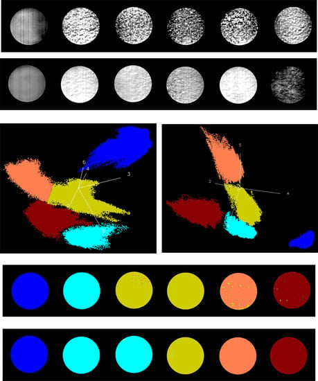
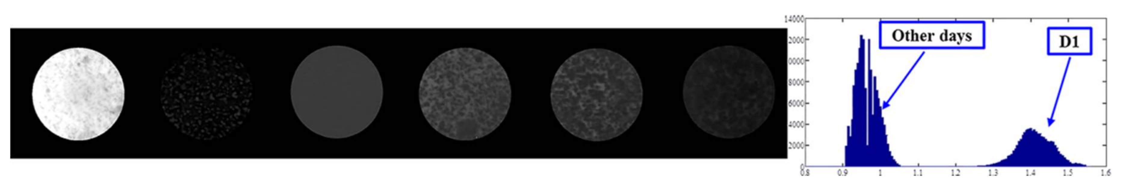
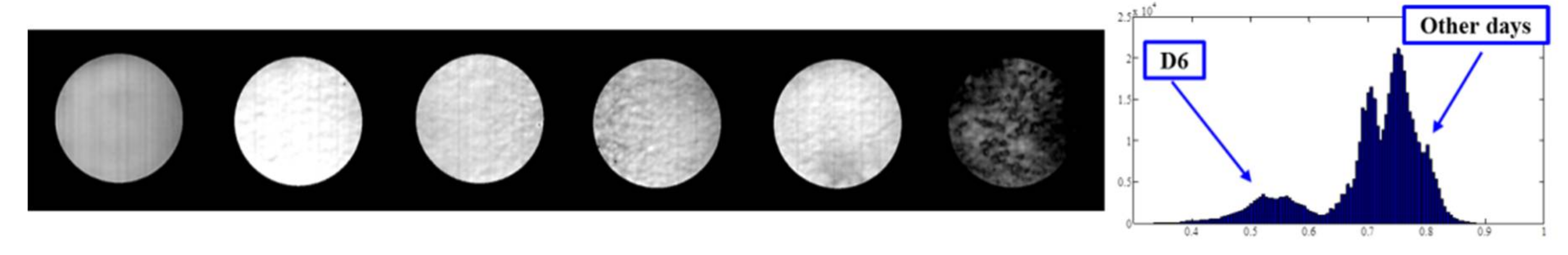
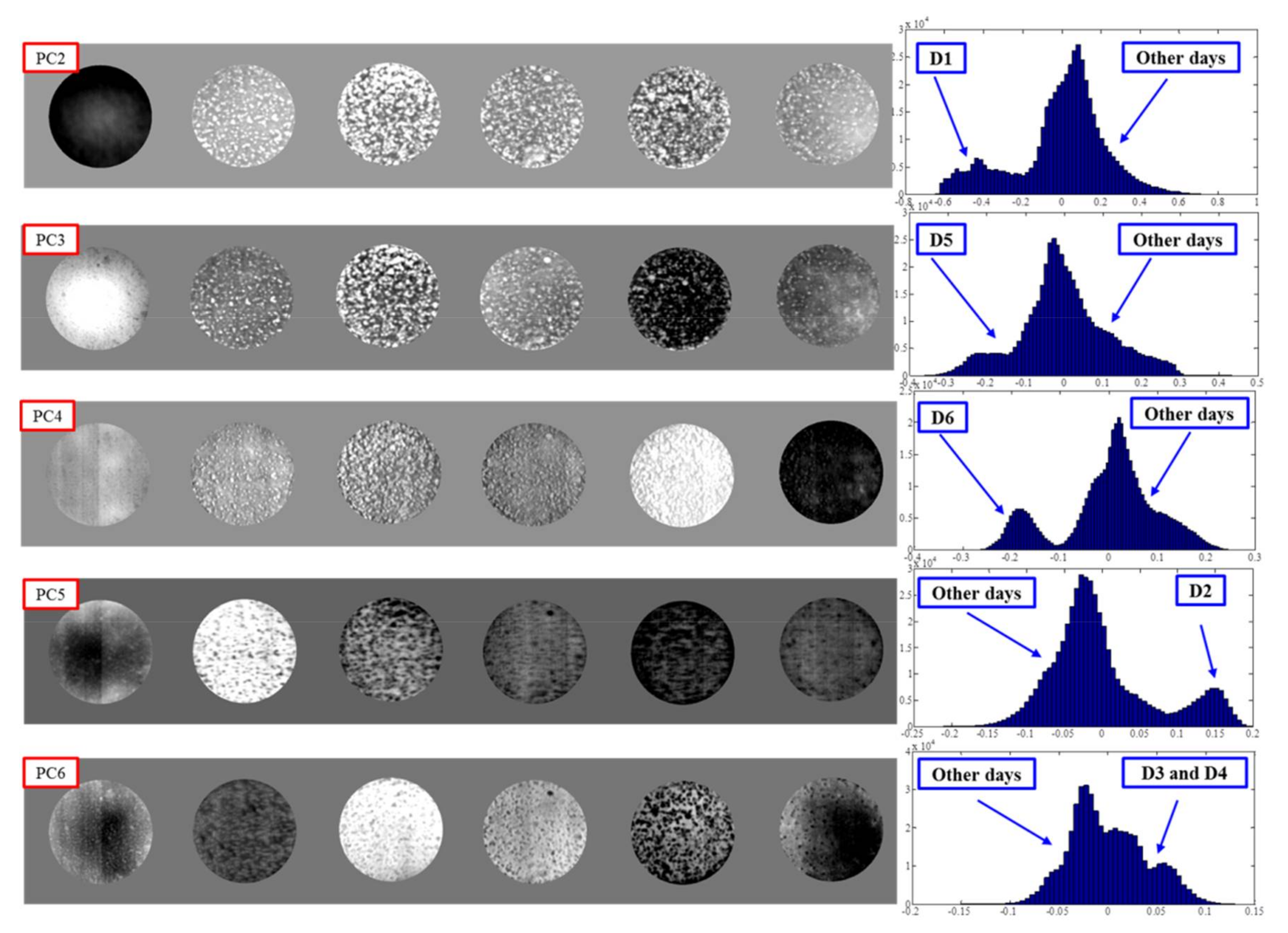
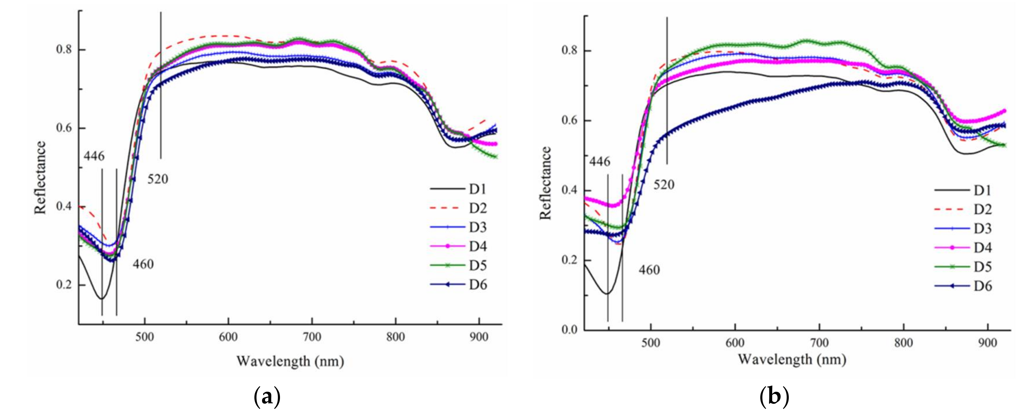
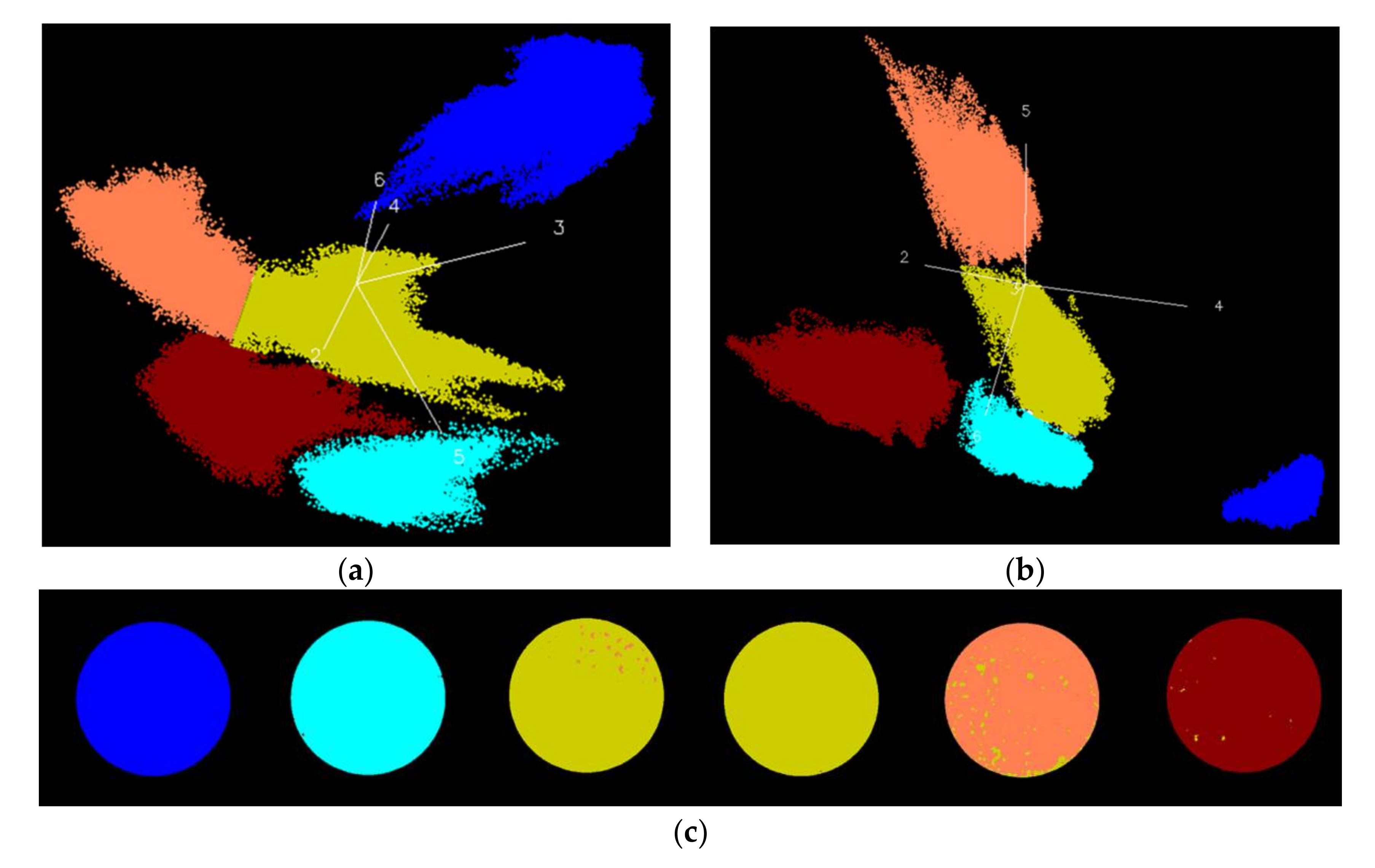
  • Band math and PCA on hyperspectral image can be used to classify fungi with distinct characteristics. A band ratio of 446 nm and 460 nm classified A. flavus and A. parasiticus on day 1. The image at the band of 520 nm classified A. parasiticus on day 6. The 5-dimensional score plot of PC2 to PC6 gave an indication of clusters fungi in the same incubation time, with the exception of A. flavus on day 3 and day 4 and A. parasiticus on day 2 and day 3.
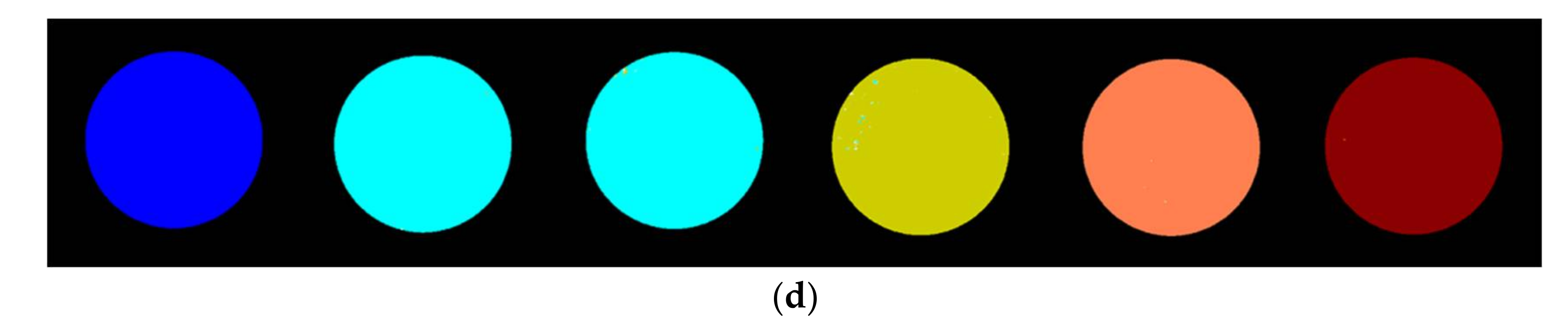
  • The SVM model that is based on full spectrum data can be used to classify fungal growth time. On the full spectral, PC2 to PC6 2–6 and the SVM method could be used to classify fungi with different incubation times. The overall classification accuracies were 92.59% and 100% for A. flavus and A. parasiticus, respectively.
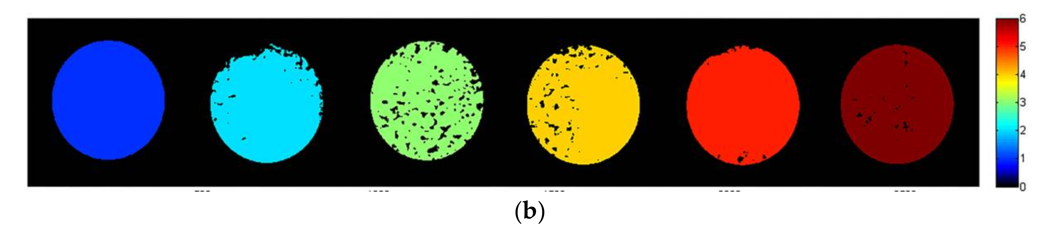
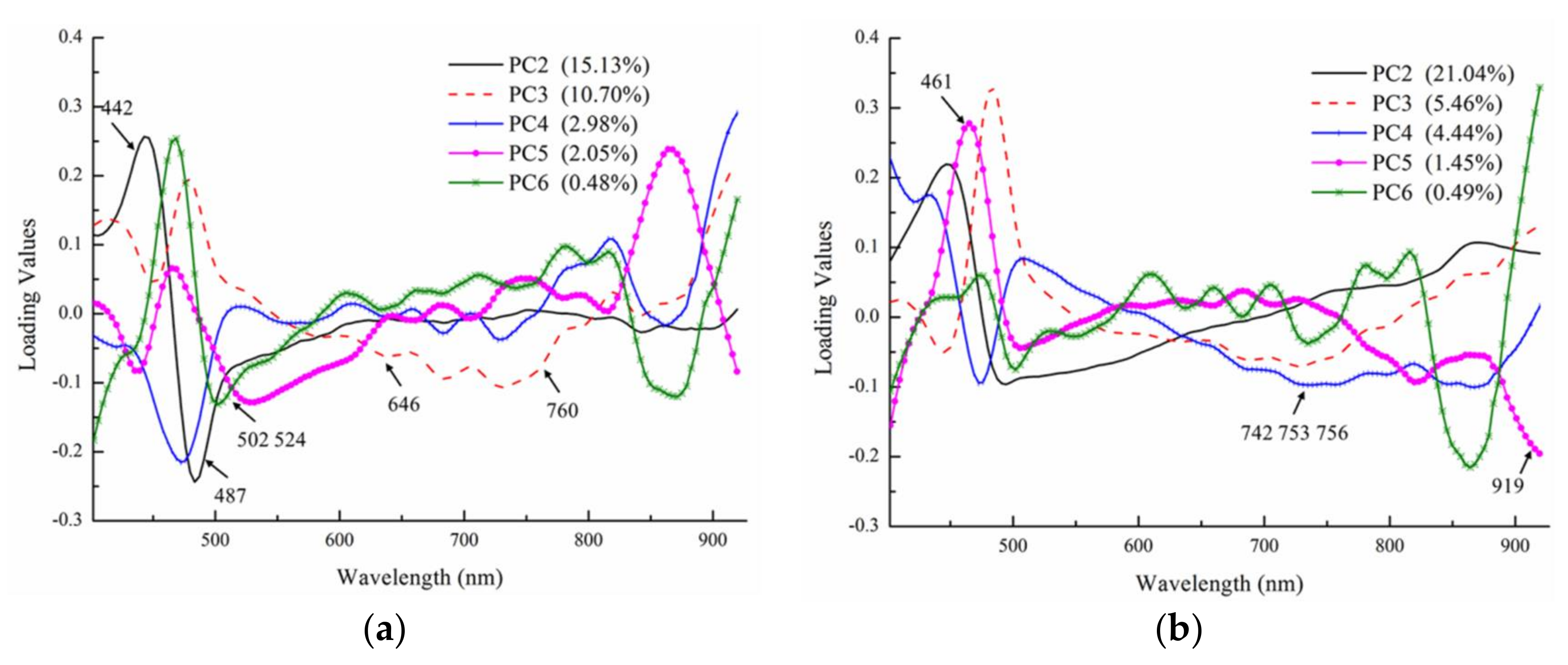
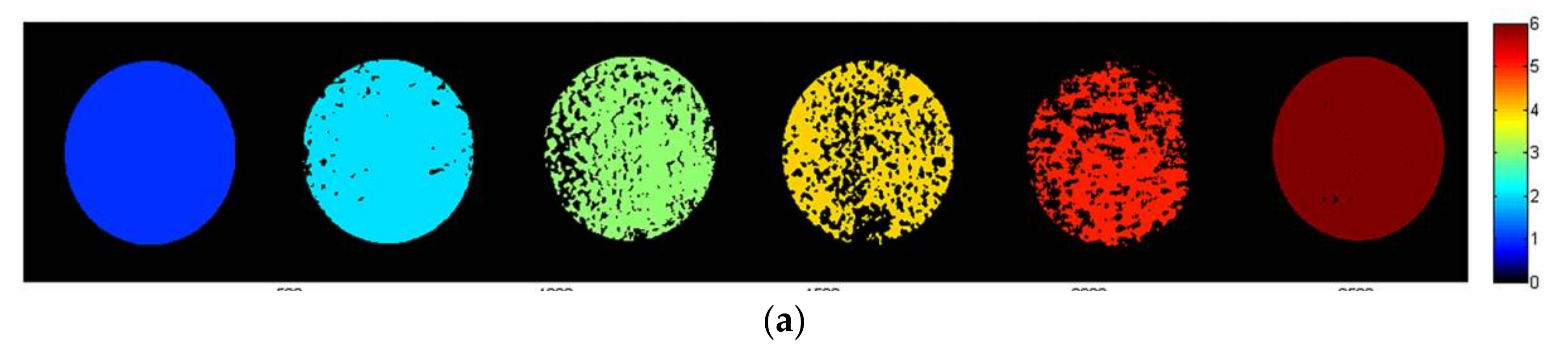
  • Optimal wavelengths selected by the CARS method can be used to a build an optimized SVM model for identifying the growth of A. flavus and A. parasiticus. Nine (402, 442, 487, 502, 524, 553, 646, 671, and 760 nm) and seven (461, 538, 542, 742, 753, 756, and 919 nm) were selected for A. flavus and A. parasiticus. The accuracies of the optimal wavelengths SVM models were 83.33% for A. flavus and 98.15% for A. parasiticus. The predicted map indicated that the predicted fungal growth days were basically consistent with the actual situation.

Acknowledgments

This study is supported by the National Natural Science Foundation of China (No. 31772062) and Fund for Less Developed Regions of the National Natural Science Foundation of China (No. 61462074).

Author Contributions

Wei Wang, Xinzhi Ni, Haitao Zheng, Ren Zhang and Yufeng Li conceived and designed the experiments; Xuan Chu and Xin Zhao performed the experiments; Xuan Chu and Xin Zhao analyzed the data; Xuan Chu and Wei Wang wrote the paper.

Conflicts of Interest

The authors declare no conflict of interest.

References

  1. Gourama, H.; Bullerman, L.B. Aspergillus flavus and Aspergillus parasiticus: Aflatoxigenic fungi of concern in foods and feeds: A Review. J. Food Prot. 1995, 58, 1395–1404. [Google Scholar] [CrossRef]
  2. Perrone, G.; Susca, A.; Cozzi, G.; Ehrlich, K.; Varga, J.; Frisvad, J.C.; Meijer, M.; Noonim, P.; Mahakarnchanakul, W.; Samson, R.A. Biodiversity of Aspergillus species in some important agricultural products. Stud. Mycol. 2007, 59, 53–66. [Google Scholar] [CrossRef] [PubMed]
  3. Kosegarten, C.E.; Ramírez-Corona, N.; Mani-López, E.; Palou, E.; López-Malo, A. Description of Aspergillus flavus growth under the influence of different factors (water activity, incubation temperature, protein and fat concentration, pH, and cinnamon essential oil concentration) by kinetic, probability of growth, and time-to-detection models. Int. J. Food Microbiol. 2017, 240, 115–123. [Google Scholar] [PubMed]
  4. Bullerman, L.B. Significance of Mycotoxins to Food Safety and Human Health. J. Food Prot. 1979, 42, 65–86. [Google Scholar] [CrossRef]
  5. Mandeel, Q.A. Fungal contamination of some imported spices. Mycopathologia 2005, 159, 291–298. [Google Scholar] [CrossRef] [PubMed]
  6. Xu, L.; Lu, Z.; Cao, L.; Pang, H.; Zhang, Q.; Fu, Y.; Xiong, Y.; Li, Y.; Wang, X.; Wang, J.; Ying, Y.; Li, Y. In-field detection of multiple pathogenic bacteria in food products using a portable fluorescent biosensing system. Food Control 2017, 75, 21–28. [Google Scholar] [CrossRef]
  7. Sun, Y.; Gu, X.; Wang, Z.; Huang, Y.; Wei, Y.; Zhang, M.; Tu, K.; Pan, L. Growth simulation and discrimination of Botrytis cinerea, Rhizopus stolonifer and Colletotrichum acutatum using hyperspectral reflectance imaging. PLoS ONE 2015, 10, e0143400. [Google Scholar] [CrossRef] [PubMed]
  8. Matcham, S.E.; Jordan, B.R.; Wood, D.A. Estimation of fungal biomass in a solid substrate by three independent methods. Appl. Microbiol. Biotechnol. 1985, 21, 108–112. [Google Scholar] [CrossRef]
  9. Edelstein, L.; Segel, L.A. Growth and metabolism in mycelial fungi. J. Theor. Biol. 1983, 104, 187–210. [Google Scholar] [CrossRef]
  10. Yoon, S.C.; Lawrence, K.C.; Siragusa, G.R.; Line, J.E.; Park, B.; Feldner, P.W. Hyperspectral reflectance imaging for detecting a foodborne pathogen: Campylobacter. Trans. ASABE 2009, 52, 651–662. [Google Scholar] [CrossRef]
  11. Kammies, T.-L.; Manley, M.; Gouws, P.A.; Williams, P.J. Differentiation of foodborne bacteria using NIR hyperspectral imaging and multivariate data analysis. Appl. Microbiol. Biotechnol. 2016, 100, 9305–9320. [Google Scholar] [CrossRef] [PubMed]
  12. Wang, L.; Pu, H.; Sun, D.-W.; Liu, D.; Wang, Q.; Xiong, Z. Application of hyperspectral imaging for prediction of textural properties of maize seeds with different storage periods. Food Anal. Methods 2015, 8, 1535–1545. [Google Scholar] [CrossRef]
  13. Yoon, S.C.; Windham, W.R.; Ladely, S.; Heitschmidt, G.W.; Lawrence, K.C.; Park, B.; Narang, N.; Cray, W.C. Differentiation of big-six non-O157 Shiga-toxin producing Escherichia coli (STEC) on spread plates of mixed cultures using hyperspectral imaging. J. Food Meas. Charact. 2013, 7, 47–59. [Google Scholar] [CrossRef]
  14. Serranti, S.; Cesare, D.; Bonifazi, G. The development of a hyperspectral imaging method for the detection of Fusarium-damaged, yellow berry and vitreous Italian durum wheat kernels. Biosyst. Eng. 2013, 115, 20–30. [Google Scholar] [CrossRef]
  15. Del Fiore, A.; Reverberi, M.; Ricelli, A.; Pinzari, F.; Serranti, S.; Fabbri, A.A.; Bonifazi, G.; Fanelli, C. Early detection of toxigenic fungi on maize by hyperspectral imaging analysis. Int. J. Food Microbiol. 2010, 144, 64–71. [Google Scholar] [CrossRef] [PubMed]
  16. Falade, T.; Sultanbawa, Y.; Fletcher, M.T.; Fox, G. Near Infrared Spectrometry for Rapid Non-Invasive Modelling of Aspergillus-Contaminated Maturing Kernels of Maize (Zea mays L.). Agriculture 2017, 7, 77. [Google Scholar] [CrossRef]
  17. Zhao, X.; Wang, W.; Chu, X.; Li, C.; Kimuli, D. Early detection of Aspergillus parasiticus infection in maize kernels using near-infrared hyperspectral imaging and multivariate data analysis. Appl. Sci. 2017, 7, 90. [Google Scholar] [CrossRef]
  18. Yao, H.; Hruska, Z.; Kincaid, R.; Brown, R.L.; Cleveland, T.E. Differentiation of toxigenic fungi using hyperspectral imagery. Sens. Instrum. Food Qual. Saf. 2008, 2, 215. [Google Scholar] [CrossRef]
  19. Jin, J.; Tang, L.; Hruska, Z.; Yao, H. Classification of toxigenic and atoxigenic strains of Aspergillus flavus with hyperspectral imaging. Comput. Electron. Agric. 2009, 69, 158–164. [Google Scholar] [CrossRef]
  20. Williams, P.J.; Geladi, P.; Britz, T.J.; Manley, M. Near-infrared (NIR) hyperspectral imaging and multivariate image analysis to study growth characteristics and differences between species and strains of members of the genus Fusarium. Anal. Bioanal. Chem. 2012, 404, 1759–1769. [Google Scholar] [CrossRef] [PubMed]
  21. Williams, P.J.; Geladi, P.; Britz, T.J.; Manley, M. Growth characteristics of three Fusarium species evaluated by near-infrared hyperspectral imaging and multivariate image analysis. Appl. Microbiol. Biotechnol. 2012, 96, 803–813. [Google Scholar] [CrossRef] [PubMed]
  22. Dégardin, K.; Guillemain, A.; Guerreiro, N.V.; Roggo, Y. Near infrared spectroscopy for counterfeit detection using a large database of pharmaceutical tablets. J. Pharm. Biomed. Anal. 2016, 128, 89–97. [Google Scholar] [CrossRef] [PubMed]
  23. Jia, B.; Yoon, S.-C.; Zhuang, H.; Wang, W.; Li, C. Prediction of pH of fresh chicken breast fillets by VNIR hyperspectral imaging. J. Food Eng. 2017, 208, 57–65. [Google Scholar] [CrossRef]
  24. Williams, P.J.; Geladi, P.; Britz, T.J.; Manley, M. Investigation of fungal development in maize kernels using NIR hyperspectral imaging and multivariate data analysis. J. Cereal Sci. 2012, 55, 272–278. [Google Scholar] [CrossRef]
  25. Kamruzzaman, M.; ElMasry, G.; Sun, D.-W.; Allen, P. Application of NIR hyperspectral imaging for discrimination of lamb muscles. J. Food Eng. 2011, 104, 332–340. [Google Scholar] [CrossRef]
  26. Li, J.; Chen, L.; Huang, W. Detection of early bruises on peaches (Amygdalus persica L.) using hyperspectral imaging coupled with improved watershed segmentation algorithm. Postharvest Biol. Technol. 2018, 135, 104–113. [Google Scholar] [CrossRef]
  27. Fan, S.; Huang, W.; Guo, Z.; Zhang, B.; Zhao, C. Prediction of soluble solids content and firmness of pears using hyperspectral reflectance imaging. Food Anal. Methods 2015, 8, 1936–1946. [Google Scholar] [CrossRef]
  28. He, H.-J.; Sun, D.-W.; Wu, D. Rapid and real-time prediction of lactic acid bacteria (LAB) in farmed salmon flesh using near-infrared (NIR) hyperspectral imaging combined with chemometric analysis. Food Res. Int. 2014, 62, 476–483. [Google Scholar] [CrossRef]
  29. Wu, D.; Sun, D.-W. Potential of time series-hyperspectral imaging (TS-HSI) for non-invasive determination of microbial spoilage of salmon flesh. Talanta 2013, 111, 39–46. [Google Scholar] [CrossRef] [PubMed]
  30. Melgani, F.; Bruzzone, L. Classification of hyperspectral remote sensing images with support vector machines. IEEE Trans. Geosci. Remote Sens. 2004, 42, 1778–1790. [Google Scholar] [CrossRef]
  31. Fernández-Ibañez, V.; Soldado, A.; Martínez-Fernández, A.; De la Roza-Delgado, B. Application of near infrared spectroscopy for rapid detection of aflatoxin B1 in maize and barley as analytical quality assessment. Food Chem. 2009, 113, 629–634. [Google Scholar] [CrossRef]
Figure 1. (a) Resized hyperspectral image; (b) mask for the hyperspectral image.
Applsci 08 00513 g001
Figure 2. (a) Average spectra of A. flavus and (b) average spectra of A. parasiticus.
Applsci 08 00513 g002
Figure 3. Band ratio image (460/446 nm) of A. flavus.
Applsci 08 00513 g003
Figure 4. Image of A. parasiticus at 520 nm.
Applsci 08 00513 g004
Figure 5. The second to sixth principal components (PC2 to PC6) images of A. flavus.
Applsci 08 00513 g005
Figure 6. (a) PC2 to PC6 score plot of A. flavus; (b) PC2 to PC6 score plot of A. parasiticus; (c) classes projected onto image of A. flavus; and (d) classes projected onto image of A. parasiticus.
Applsci 08 00513 g006aApplsci 08 00513 g006b
Figure 7. Location of regions of interest (ROI) on a Petri dish.
Applsci 08 00513 g007
Figure 8. (a) Loading line plot of A. flavus and (b) loading line plot of A. parasiticus.
Applsci 08 00513 g008
Figure 9. (a) Prediction images of A. flavus and (b) prediction images of A. parasiticus.
Applsci 08 00513 g009aApplsci 08 00513 g009b

