Assessment of Student Music Performances Using Deep Neural Networks


Abstract
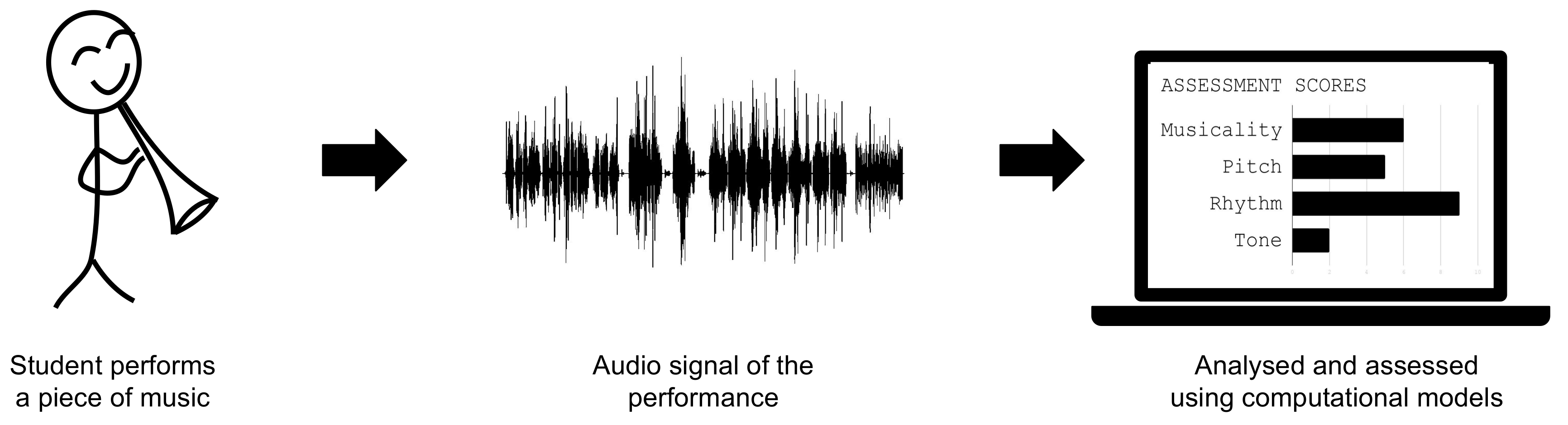
1. Introduction
2. Related Work
3. Material and Methods
3.1. Dataset
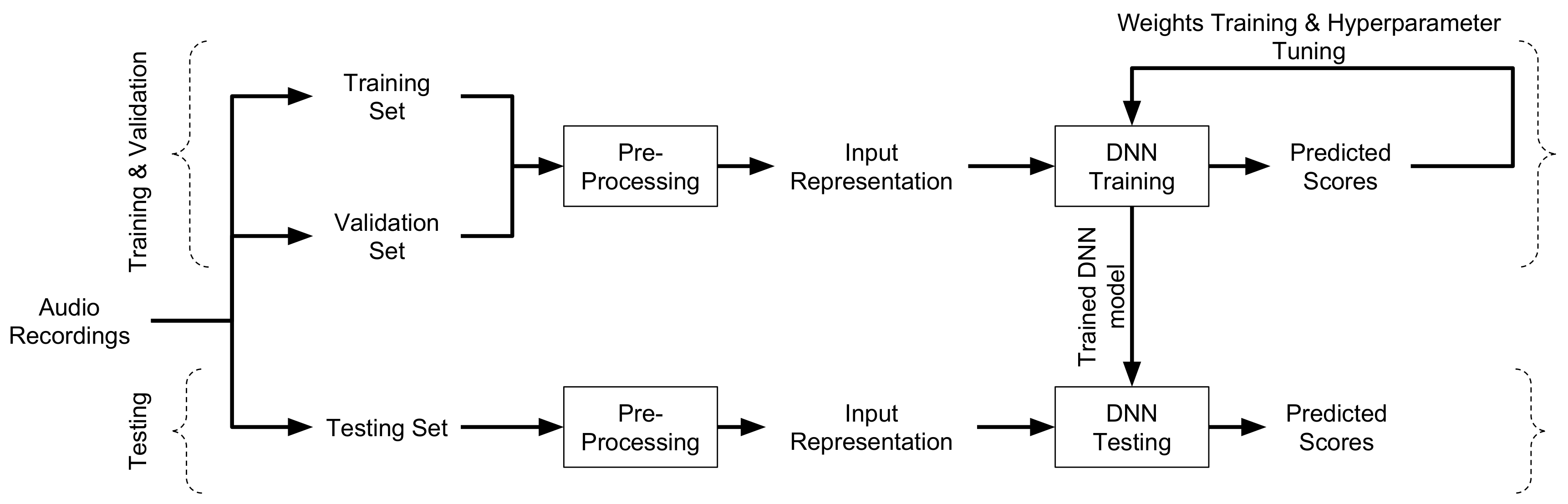
3.2. System Overview
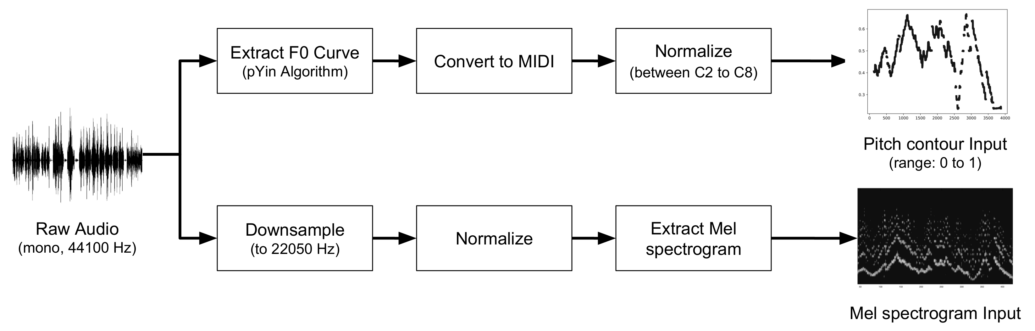
3.3. Pre-Processing
3.3.1. Pitch Contour
3.3.2. Mel Spectrogram
3.4. Deep Neural Network Architectures
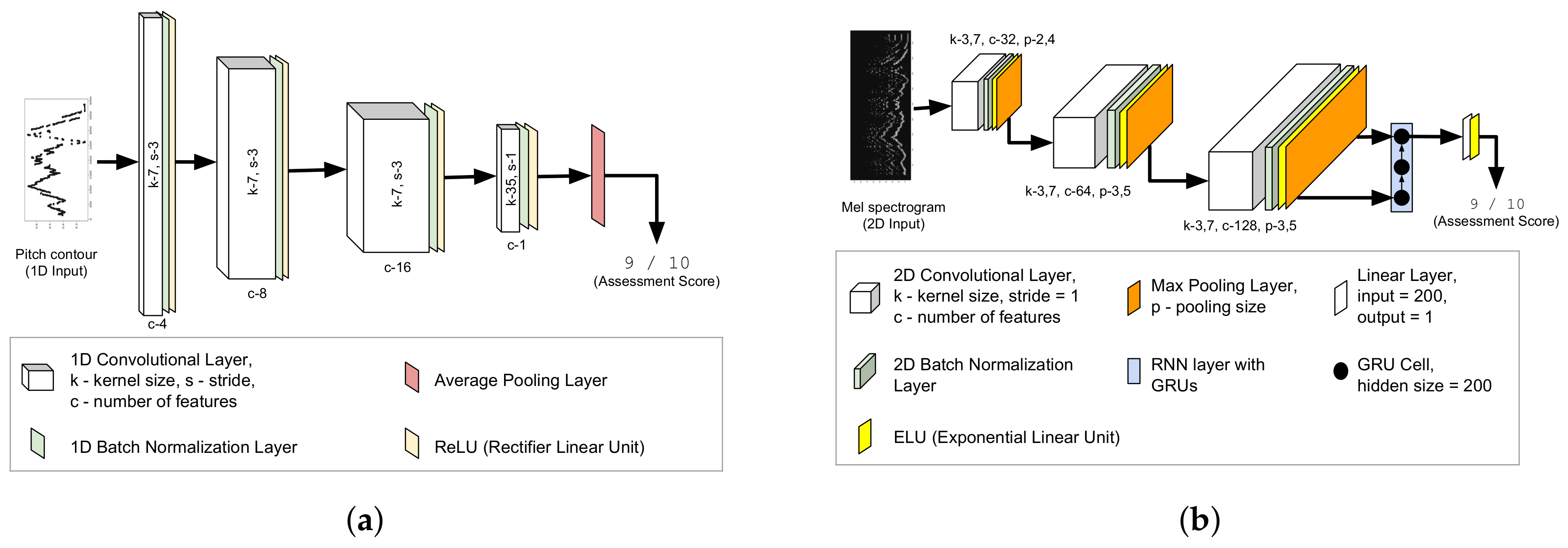
3.4.1. Fully Convolutional Pitch Contour Model
3.4.2. Convolutional Recurrent Model with Mel Spectrogram
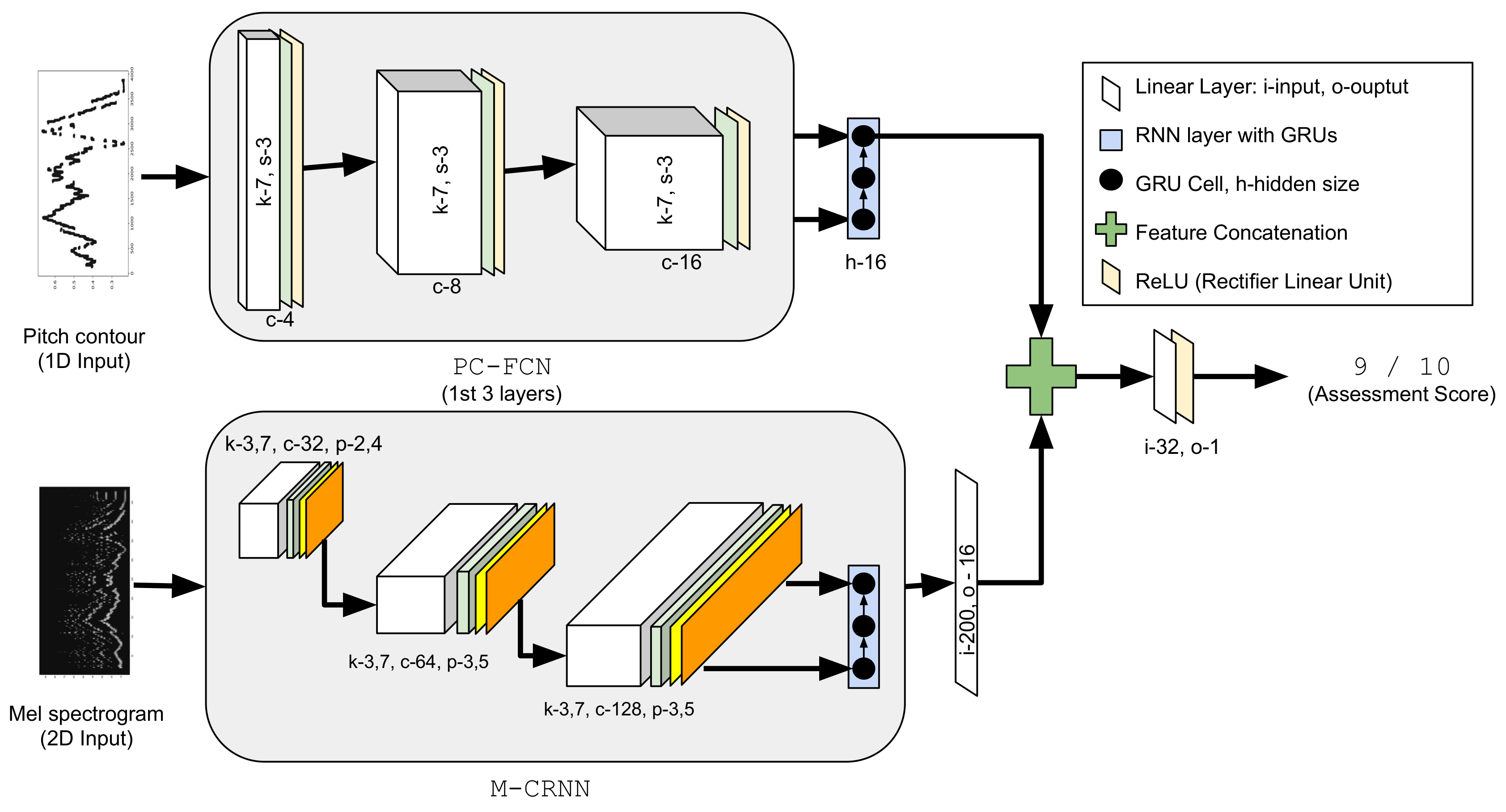
3.4.3. Hybrid Model Combining Mel-Spectrogram and Pitch Contour Inputs
3.5. Deep Neural Network Training Procedure
3.6. Experiments
- (i)
- SVR-BD: SVR model using a feature set that combines both low-level and hand-crafted features. The low-level features are comprised of standard spectral and temporal features such as MFCCs, spectral flux, spectral centroid, spectral roll-off, zero-crossing rate, etc. The hand-crafted features, on the other hand, model note-level features such as note steadiness and amplitude deviations, as well as performance level features such as average accuracy, percentage of correct notes, and timing accuracy. The dimensionality of the combined feature set is 92 (68 for low-level, 24 for hand-crafted).
- (ii)
- PC-FCN: Fully convolutional model with the PC representation as the input.
- (iii)
- M-CRNN: Convolutional recurrent model with the MEL representation as the input.
- (iv)
- PCM-CRNN: Hybrid model that leverages both the PC and MEL input representations.
3.7. Evaluation Metrics
4. Results
- (i)
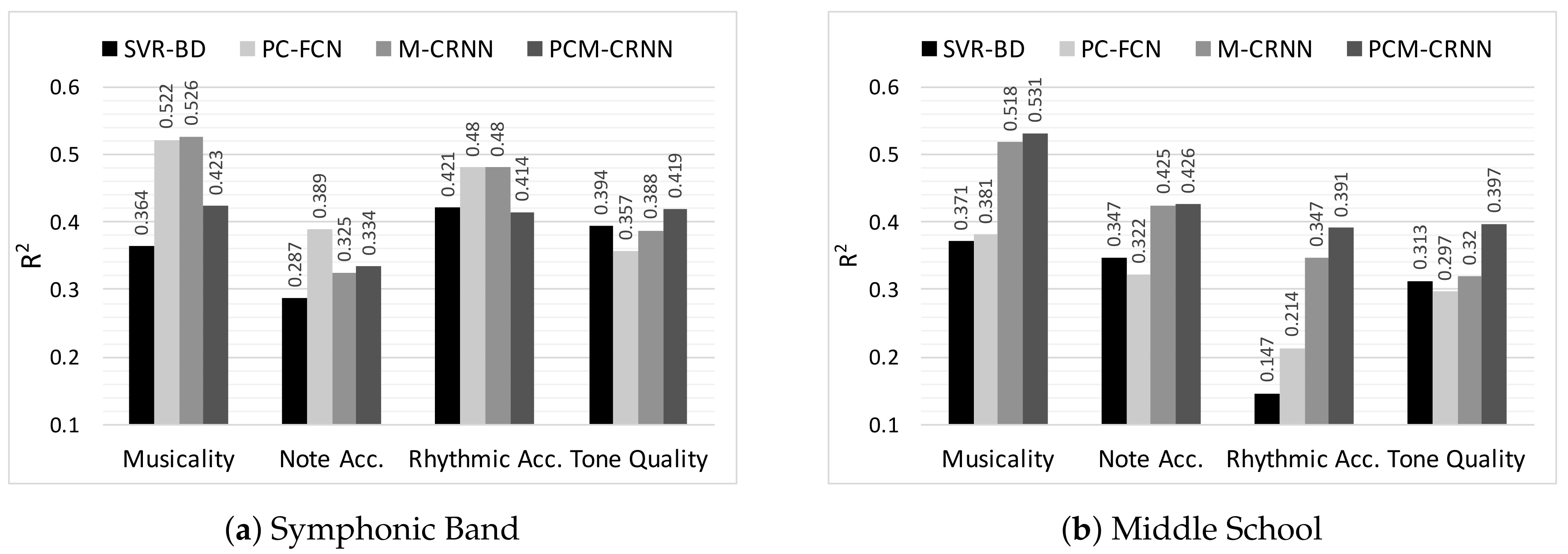
- For both student categories and for all assessment criteria, the SVR model is always outperformed by at least one of the DNN models. This holds true for both evaluation metrics. This suggests that deep architectures are able to extract more (musically) meaningful information from the data than standard and hand-crafted features.
- (ii)
- The best performance is observed for the assessment of Musicality. For both student categories, the best DNN models show clear superior performance compared to the SVR-BD model. It is worth noting that, among all the assessment criteria, Musicality is probably the most abstract and difficult to define. This makes feature engineering for Musicality rather difficult. The better performance of DNNs at this assessment criterion further indicates the capability of feature learning methods to model abstract concepts by learning patterns in data. Within the DNN models, those using RNNs consistently perform better for both student categories (except for PCM-CRNN for Symphonic Band). This shows the benefits of capturing temporal information for modeling this assessment criterion.
- (iii)
- The PC-FCN model outperforms the other DNN models in the case of Note Accuracy for the Symphonic Band. As Symphonic Band students show a generally higher musical proficiency than Middle School students, one possible reason for this could be that as the proficiency level of the students increases, the high level melodic information encoded in the pitch contour becomes more important in the assessment process. It is also worth noting that the musical scores performed by the Symphonic Band students are considerably more complex than the Middle School students in terms of note density and distribution across the scales. We discuss this further in Section 5.
- (iv)
- For the Tone Quality criterion, the DNN models show only minor improvement over the baseline SVR-BD model. This could possibly be explained by the spectral features (MFCCs, etc.), which are already very efficient at capturing timbral information and, thus, cannot be easily outperformed by learned features. The relatively poor performance of PC-FCN at this criterion is expected, given that the pitch contour computation process discards all timbre information; hence, the model has no relevant information to begin with. However, the performance of the MEL input based models (M-CRNN and PCM-CRNN) suggests that DNNs are able to learn useful features for this criteria from the MEL input representation.
- (v)
- For Middle School, the PCM-CRNN hybrid model performs at par or better than all other models and across all assessment criteria. This is expected since it observes both high level and low level representations as input and therefore draws from more data to learn better features. However, the performance of this model falls below expectation in the first three assessment criteria for Symphonic Band. This requires further investigation as there is no obvious explanation.
5. Model Analysis
6. Conclusions
- (i)
- We introduce DNN based architectures for the music performance assessment task. The experimental results show the overall promise of using supervised feature learning methods for this task and the shortcomings of traditional approaches in describing music performances.
- (ii)
- We compare and contrast input data representations at different levels of abstraction and show that information encoded by each is critical for different assessment criteria.
- (iii)
- Compared to the baseline, we are able to show considerable improvement in model performance. For Musicality, which is arguably the most abstract assessment criterion, we demonstrate clear superior performance of the DNN models.
- (iv)
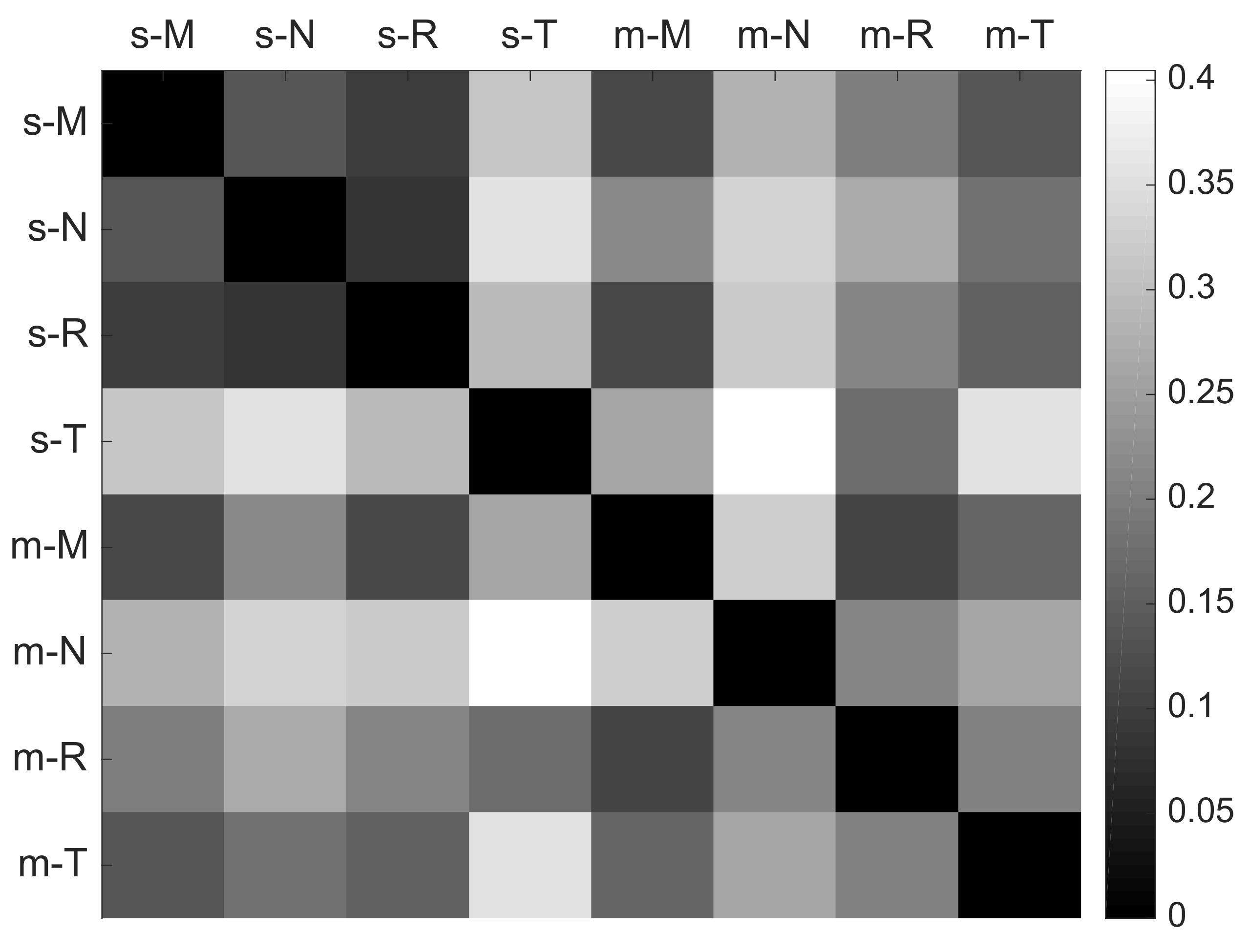
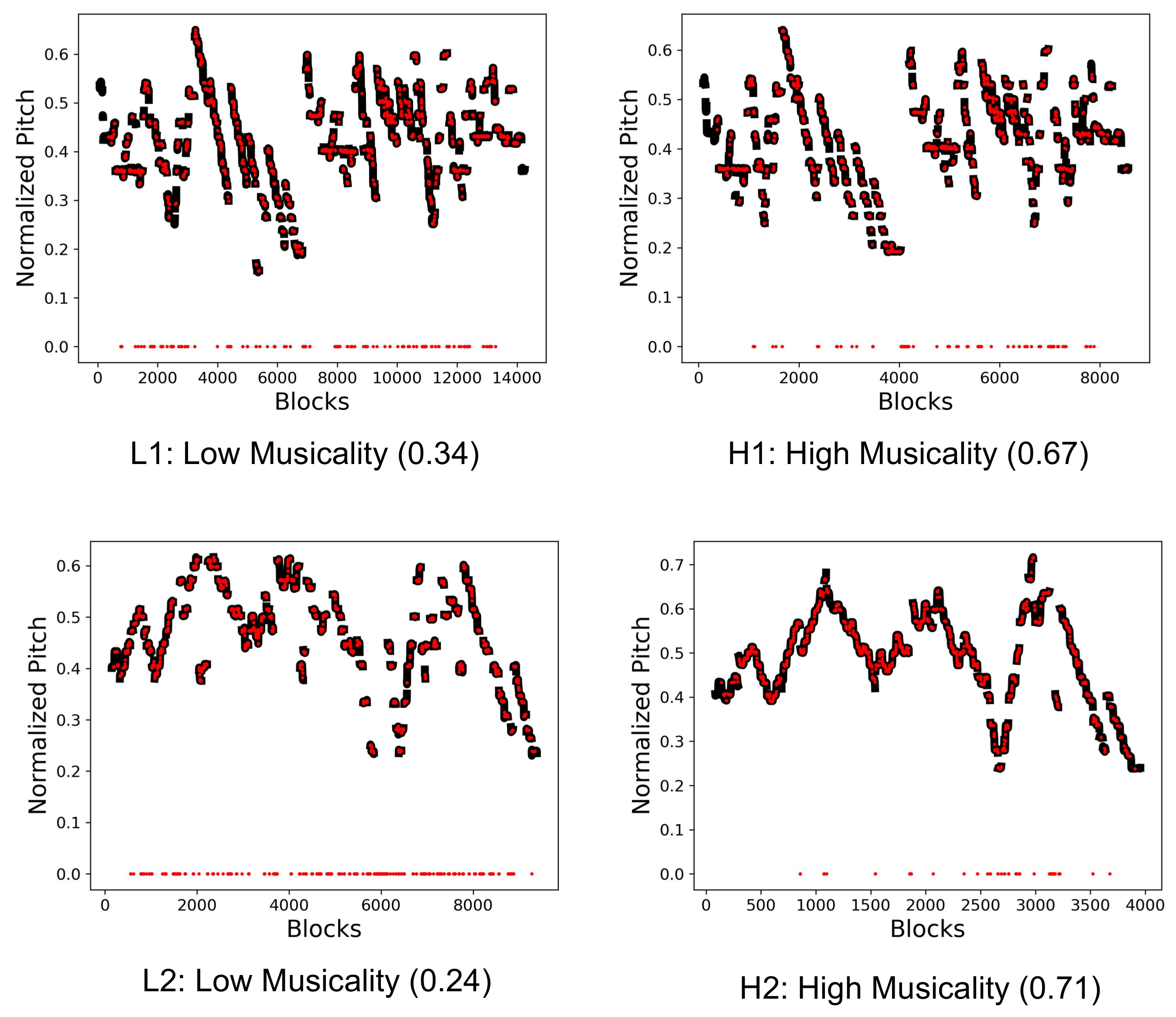
- We use model analysis techniques such as filter distance measures and saliency maps to explain the model predictions and further our understanding of the performance assessment process in general.
- (i)
- Developing better input representations: Constant Q-Transforms have shown good results with other MIR tasks [28] and are thus a potential candidate for a low level representation. In addition, augmenting the pitch contours with the amplitude variations or pitch saliency could be a simple and yet effective way to encode dynamics. Another potential direction could be to switch to a raw time-domain input representation. While input representations help condense information, which facilitates feature learning, information that might be otherwise useful is discarded during their computation process. Examples include the loss of timbral and dynamic information during the pitch extraction process or the loss of the phase in a magnitude spectrum. Therefore, learning from raw audio—though challenging—presents opportunities to not only improve the performance of the models at this task, but also further our understanding of music perception in general.
- (ii)
- Adding the musical score: Although the human judges have access to the score that the students are performing, the DNN models do not. It would be of interest to design a model that allows encoding the score information in the input representation.
- (iii)
- Improving the training data: While we use the concept of weak labels to improve model training by increasing the amount of data available, other more popular data augmentation methods such as pitch shifting can be used to potentially increase the models’ robustness. Adding performances from other instruments to increase the available data is also an option, but requires adequate care to avoid bias towards a particular class of instruments. Given enough data, an alternative option would be to train instrument specific models, which can then capture the nuances and assessment criteria of the individual instruments better.
- (iv)
- Modifying the training methodology: Since the models are trained on one dataset with a limited number of instruments, they cannot be directly used on other music performance datasets. However, based on our preliminary cross-category analysis results, transfer learning [71] could be an option for certain assessment criteria and warrants further investigation.
- (v)
- Investigating alternative model analysis techniques: Along with the techniques used in this article, other model analysis techniques such as layer-wise relevance propagation [70] can be explored to further improve our understanding of the feature learning process. Improving the interpretability of DNNs is an active area of research in the Artificial Intelligence community and more efforts are needed to build better tools targeting music and general audio-based tasks.
- (vi)
- Combining multiple modalities: A music performance mostly caters to the auditory sense. However, visual cues such as gestures form a significant component of a music performance, which might influence the perception of expressiveness [72,73]. Using multi-modal input representations, which encode both auditory and visual information can provide several interesting possibilities for future research.
Acknowledgments
Author Contributions
Conflicts of Interest
References
- Palmer, C. Music performance. Ann. Rev. Psychol. 1997, 48, 115–138. [Google Scholar] [CrossRef] [PubMed]
- Bloom, B.S. Taxonomy of Educational Objectives; McKay: New York, NY, USA, 1956; pp. 20–24. [Google Scholar]
- Wesolowski, B.C.; Wind, S.A.; Engelhard, G. Examining rater precision in music performance assessment: An analysis of rating scale structure using the Multifaceted Rasch Partial Credit Model. Music Percept. 2016, 33, 662–678. [Google Scholar] [CrossRef]
- Thompson, S.; Williamon, A. Evaluating evaluation: Musical performance assessment as a research tool. Music Percept. 2003, 21, 21–41. [Google Scholar] [CrossRef]
- Schedl, M.; Gómez, E.; Urbano, J. Music information retrieval: Recent developments and applications. Found. Trends Inf. Retr. 2014, 8, 127–261. [Google Scholar] [CrossRef]
- De Cheveigné, A.; Kawahara, H. YIN, a fundamental frequency estimator for speech and music. J. Acoust. Soc. Am. 2002, 111, 1917–1930. [Google Scholar] [CrossRef] [PubMed]
- Gerhard, D. Pitch Extraction and Fundamental Frequency: History and Current Techniques; TR-CS 2003-06; Department of Computer Science, University of Regina: Regina, SK, Canada, 2003. [Google Scholar]
- Benetos, E.; Dixon, S.; Giannoulis, D.; Kirchhoff, H.; Klapuri, A. Automatic music transcription: Challenges and future directions. J. Intell. Inf. Syst. 2013, 41, 407–434. [Google Scholar] [CrossRef]
- Ryynänen, M.P.; Klapuri, A.P. Automatic transcription of melody, bass line, and chords in polyphonic music. Comput. Music J. 2008, 32, 72–86. [Google Scholar] [CrossRef]
- Huang, P.S.; Kim, M.; Hasegawa-Johnson, M.; Smaragdis, P. Singing-Voice Separation from Monaural Recordings using Deep Recurrent Neural Networks. In Proceedings of the International Society of Music Information Retrieval Conference (ISMIR), Taipei, Taiwan, 27–31 October 2014; pp. 477–482. [Google Scholar]
- Nakano, T.; Goto, M.; Hiraga, Y. An automatic singing skill evaluation method for unknown melodies using pitch interval accuracy and vibrato features. In Proceedings of the International Conference on Spoken Language Processing (ICSLP), Pittsburgh, PA, USA, 17–21 September 2006; pp. 1706–1709. [Google Scholar]
- Knight, T.; Upham, F.; Fujinaga, I. The potential for automatic assessment of trumpet tone quality. In Proceedings of the International Society of Music Information Retrieval Conference (ISMIR), Miami, FL, USA, 24–18 October 2011; pp. 573–578. [Google Scholar]
- Dittmar, C.; Cano, E.; Abeßer, J.; Grollmisch, S. Music Information Retrieval Meets Music Education. In Multimodal Music Processing; Müller, M., Goto, M., Schedl, M., Eds.; Dagstuhl Follow-Ups Series; Schloss Dagstuhl-Leibniz-Zentrum fuer Informatik: Wadern, Germany, 2012; Volume 3. [Google Scholar]
- Abeßer, J.; Hasselhorn, J.; Dittmar, C.; Lehmann, A.; Grollmisch, S. Automatic quality assessment of vocal and instrumental performances of ninth-grade and tenth-grade pupils. In Proceedings of the International Symposium on Computer Music Multidisciplinary Research (CMMR), Marseille, France, 15–18 October 2013. [Google Scholar]
- Romani Picas, O.; Parra Rodriguez, H.; Dabiri, D.; Tokuda, H.; Hariya, W.; Oishi, K.; Serra, X. A Real-Time System for Measuring Sound Goodness in Instrumental Sounds. In Proceedings of the 138th Audio Engineering Society Convention, Warsaw, Poland, 7–10 May 2015. [Google Scholar]
- Luo, Y.J.; Su, L.; Yang, Y.H.; Chi, T.S. Detection of Common Mistakes in Novice Violin Playing. In Proceedings of the International Society of Music Information Retrieval Conference (ISMIR), Taipei, Taiwan, 27–31 October 2015; pp. 316–322. [Google Scholar]
- Li, P.C.; Su, L.; Yang, Y.H.; Su, A.W. Analysis of Expressive Musical Terms in Violin Using Score-Informed and Expression-Based Audio Features. In Proceedings of the International Society of Music Information Retrieval Conference (ISMIR), Taipei, Taiwan, 27–31 October 2015; pp. 809–815. [Google Scholar]
- Wu, C.W.; Gururani, S.; Laguna, C.; Pati, A.; Vidwans, A.; Lerch, A. Towards the Objective Assessment of Music Performances. In Proceedings of the International Conference on Music Perception and Cognition (ICMPC), San Francisco, CA, USA, 5–9 July 2016; pp. 99–103. [Google Scholar]
- Vidwans, A.; Gururani, S.; Wu, C.W.; Subramanian, V.; Swaminathan, R.V.; Lerch, A. Objective descriptors for the assessment of student music performances. In Proceedings of the AES International Conference on Semantic Audio, Audio Engineering Society, Erlangen, Germany, 22–24 June 2017. [Google Scholar]
- Bozkurt, B.; Baysal, O.; Yuret, D. A Dataset and Baseline System for Singing Voice Assessment. In Proceedings of the International Symposium on Computer Music Multidisciplinary Research (CMMR), Matosinhos, Portugal, 25–28 September 2017; pp. 430–438. [Google Scholar]
- Yousician. Available online: https://www.yousician.com (accessed on 28 February 2018).
- Smartmusic. Available online: https://www.smartmusic.com (accessed on 28 February 2018).
- Wu, C.W.; Lerch, A. Learned Features for the Assessment of Percussive Music Performances. In Proceedings of the International Conference on Semantic Computing (ICSC), Laguna Hills, CA, USA, 31 January–2 February 2018. [Google Scholar]
- Csáji, B.C. Approximation with Artificial Neural Networks. Master’s Thesis, Etvs Lornd University, Budapest, Hungary, 2001. [Google Scholar]
- Choi, K.; Fazekas, G.; Sandler, M.; Cho, K. Convolutional recurrent neural networks for music classification. In Proceedings of the International Conference on Acoustics, Speech and Signal Processing (ICASSP), New Orleans, LA, USA, 5–9 March 2017; pp. 2392–2396. [Google Scholar]
- Chandna, P.; Miron, M.; Janer, J.; Gómez, E. Monoaural audio source separation using deep convolutional neural networks. In Proceedings of the International Conference on Latent Variable Analysis and Signal Separation (LVA/ICA), Grenoble, France, 21–23 Feburary 2017; pp. 258–266. [Google Scholar]
- Luo, Y.; Chen, Z.; Hershey, J.R.; Le Roux, J.; Mesgarani, N. Deep clustering and conventional networks for music separation: Stronger together. In Proceedings of the International Conference on Acoustics, Speech and Signal Processing (ICASSP), New Orleans, LA, USA, 5–9 March 2017; pp. 61–65. [Google Scholar]
- Bittner, R.M.; McFee, B.; Salamon, J.; Li, P.; Bello, J.P. Deep salience representations for f0 estimation in polyphonic music. In Proceedings of the International Society for Music Information Retrieval Conference (ISMIR), Suzhou, China, 23–27 October 2017; pp. 23–27. [Google Scholar]
- Clarke, E. Understanding the Psychology of Performance. In Musical Performance: A Guide to Understanding; Cambridge University Press: Cambridge, UK, 2002; pp. 59–72. [Google Scholar]
- Lerch, A. Software-Based Extraction of Objective Parameters From Music Performances. Ph.D. Thesis, Technical University of Berlin, Berlin, Germany, 2008. [Google Scholar]
- Palmer, C. Mapping musical thought to musical performance. J. Exp. Psychol. 1989, 15, 331. [Google Scholar] [CrossRef]
- Repp, B.H. Patterns of note onset asynchronies in expressive piano performance. J. Acoust. Soc. Am. 1996, 100, 3917–3932. [Google Scholar] [CrossRef] [PubMed]
- Dixon, S.; Goebl, W. Pinpointing the beat: Tapping to expressive performances. In Proceedings of the 7th International Conference on Music Perception and Cognition (ICMPC), Sydney, Australia, 17–21 July 2002; pp. 617–620. [Google Scholar]
- Seashore, C.E. The psychology of music. Music Educ. J. 1936, 23, 20–22. [Google Scholar] [CrossRef]
- Allvin, R.L. Computer-assisted music instruction: A look at the potential. J. Res. Music Educ. 1971, 19, 131–143. [Google Scholar] [CrossRef]
- Humphrey, E.J.; Bello, J.P.; LeCun, Y. Moving Beyond Feature Design: Deep Architectures and Automatic Feature Learning in Music Informatics. In Proceedings of the International Soceity of Music Information Retrieval Conference (ISMIR), Porto, Portugal, 8–12 October 2012; pp. 403–408. [Google Scholar]
- LeCun, Y.; Bengio, Y. Convolutional networks for images, speech, and time series. In The Handbook of Brain Theory and Neural Networks; MIT Press: Cambridge, MA, USA, 1995. [Google Scholar]
- Krizhevsky, A.; Sutskever, I.; Hinton, G.E. Imagenet classification with deep convolutional neural networks. In Proceedings of the Advances in Neural Information Processing Systems (NIPS), Lake Tahoe, NV, USA, 3–8 December 2012; pp. 1097–1105. [Google Scholar]
- Sainath, T.N.; Mohamed, A.-R.; Kingsbury, B.; Ramabhadran, B. Deep convolutional neural networks for LVCSR. In Proceedings of the 2013 IEEE International Conference on Acoustics, Speech and Signal Processing (ICASSP), Vancouver, BC, Canada, 26–31 May 2013; pp. 8614–8618. [Google Scholar]
- Ullrich, K.; Schlüter, J.; Grill, T. Boundary Detection in Music Structure Analysis using Convolutional Neural Networks. In Proceedings of the International Society for Music Information Retrieval Conference (ISMIR), Utrecht, The Netherlands, 9–13 August 2014; pp. 417–422. [Google Scholar]
- Choi, K.; Fazekas, G.; Sandler, M. Automatic tagging using deep convolutional neural networks. In Proceedings of the International Society of Music Information Retrieval Conference (ISMIR), New York City, NY, USA, 8–11 August 2016; pp. 805–811. [Google Scholar]
- Korzeniowski, F.; Widmer, G. A fully convolutional deep auditory model for musical chord recognition. In Proceedings of the International Workshop on Machine Learning for Signal Processing (MLSP), Salerno, Italy, 13–16 September 2016; pp. 1–6. [Google Scholar]
- Medsker, L.; Jain, L. Recurrent neural networks. In Design and Applications; CRC Press: London, UK, 2001. [Google Scholar]
- Sigtia, S.; Benetos, E.; Dixon, S. An end-to-end neural network for polyphonic piano music transcription. IEEE/ACM Trans. Audio Speech Lang. Process. 2016, 24, 927–939. [Google Scholar] [CrossRef]
- Han, Y.; Lee, K. Hierarchical approach to detect common mistakes of beginner flute players. In Proceedings of the International Society of Music Information Retrieval Conference (ISMIR), Curitiba, Brazil, 4–8 November 2014; pp. 77–82. [Google Scholar]
- Olshausen, B.A.; Field, D.J. Sparse coding with an overcomplete basis set: A strategy employed by V1? Vis. Res. 1997, 37, 3311–3325. [Google Scholar] [CrossRef]
- Harpur, G.F.; Prager, R.W. Development of low entropy coding in a recurrent network. Comput. Neural Syst. 1996, 7, 277–284. [Google Scholar] [CrossRef] [PubMed]
- Ngiam, J.; Chen, Z.; Bhaskar, S.A.; Koh, P.W.; Ng, A.Y. Sparse filtering. In Proceedings of the Advances in Neural Information Processing Systems (NIPS), Granada, Spain, 12–17 December 2011; pp. 1125–1133. [Google Scholar]
- Salamon, J.; Gómez, E. Melody extraction from polyphonic music signals using pitch contour characteristics. IEEE/ACM Trans. Audio Speech Lang. Process. 2012, 20, 1759–1770. [Google Scholar] [CrossRef]
- Bregman, A.S. Auditory Scene Analysis: The Perceptual Organization of Sound; MIT Press: Cambridge, MA, USA, 1990. [Google Scholar]
- Bittner, R.M.; Salamon, J.; Bosch, J.J.; Bello, J.P. Pitch Contours as a Mid-Level Representation for Music Informatics. In Proceedings of the AES International Conference on Semantic Audio, Audio Engineering Society, Erlangen, Germany, 22–24 June 2017. [Google Scholar]
- Mauch, M.; Dixon, S. pYIN: A fundamental frequency estimator using probabilistic threshold distributions. In Proceedings of the IEEE International Conference on Acoustics, Speech and Signal Processing (ICASSP), Florence, Italy, 4–9 May 2014; pp. 659–663. [Google Scholar]
- Moore, B.C. An Introduction to the Psychology of Hearing; Brill: Leiden, The Netherlands, 2012. [Google Scholar]
- Schluter, J.; Bock, S. Improved musical onset detection with convolutional neural networks. In Proceedings of the IEEE International Conference on Acoustics, Speech and Signal Processing (ICASSP), Florence, Italy, 4–9 May 2014; pp. 6979–6983. [Google Scholar]
- Van den Oord, A.; Dieleman, S.; Schrauwen, B. Deep content-based music recommendation. In Proceedings of the Advances in Neural Information Processing Systems (NIPS), Lake Tahoe, NV, USA, 4–11 December 2013; pp. 2643–2651. [Google Scholar]
- McFee, B.; Raffel, C.; Liang, D.; Ellis, D.P.; McVicar, M.; Battenberg, E.; Nieto, O. Librosa: Audio and music signal analysis in python. In Proceedings of the 14th Python in Science Conference, Austin, TX, USA, 6–12 July 2015; pp. 18–25. [Google Scholar]
- Matan, O.; Burges, C.J.; LeCun, Y.; Denker, J.S. Multi-digit recognition using a space displacement neural network. In Proceedings of the Advances in Neural Information Processing Systems (NIPS), San Francisco, CA, USA, 30 November–3 December 1992; pp. 488–495. [Google Scholar]
- Wolf, R.; Platt, J.C. Postal address block location using a convolutional locator network. In Proceedings of the Advances in Neural Information Processing Systems, Denver, CO, USA, 28 November–1 December 1994; pp. 745–752. [Google Scholar]
- Long, J.; Shelhamer, E.; Darrell, T. Fully convolutional networks for semantic segmentation. In Proceedings of the Conference on Computer Vision and Pattern Recognition (CVPR), Boston, MA, USA, 7–12 June 2015; pp. 3431–3440. [Google Scholar]
- Ioffe, S.; Szegedy, C. Batch normalization: Accelerating deep network training by reducing internal covariate shift. In Proceedings of the International Conference on Machine Learning (ICML), New York City, NY, USA, 19–24 June 2015; pp. 448–456. [Google Scholar]
- Tang, D.; Qin, B.; Liu, T. Document modeling with gated recurrent neural network for sentiment classification. In Proceedings of the 2015 Conference on Empirical Methods in Natural Language Processing (EMNLP), Lisbon, Portugal, 17–21 September 2015; pp. 1422–1432. [Google Scholar]
- Zuo, Z.; Shuai, B.; Wang, G.; Liu, X.; Wang, X.; Wang, B.; Chen, Y. Convolutional recurrent neural networks: Learning spatial dependencies for image representation. In Proceedings of the Conference on Computer Vision and Pattern Recognition Workshop (CVPRW), Boston, MA, USA, 7–12 June 2015; pp. 18–26. [Google Scholar]
- Chung, J.; Gulcehre, C.; Cho, K.; Bengio, Y. Empirical evaluation of gated recurrent neural networks on sequence modeling. arXiv. 2014. Available online: https://arxiv.org/abs/1412.3555 (accessed on 28 February 2018).
- Jozefowicz, R.; Zaremba, W.; Sutskever, I. An empirical exploration of recurrent network architectures. In Proceedings of the International Conference on Machine Learning, Lille, France, 6–11 July 2015; pp. 2342–2350. [Google Scholar]
- Paszke, A.; Gross, S.; Chintala, S.; Chanan, G. PyTorch: Tensors and dynamic neural networks in Python with strong GPU Acceleration. Available online: http://pytorch.org (accessed on 28 February 2018).
- Pati, K.A.; Gururani, S. MusicPerfAssessment. Available online: https://github.com/ashispati/MusicPerfAssessment (accessed on 28 February 2018).
- Kingma, D.P.; Ba, J. Adam: A method for stochastic optimization. arXiv. 2014. Available online: https://arxiv.org/abs/1412.6980 (accessed on 28 February 2018).
- McClave, J.T.; Sincich, T. Statistics, 9th ed.; Prentice Hall: Upper Saddle River, NJ, USA, 2003. [Google Scholar]
- Simonyan, K.; Vedaldi, A.; Zisserman, A. Deep inside convolutional networks: Visualising image classification models and saliency maps. arXiv. 2013. Available online: https://arxiv.org/abs/1312.6034 (accessed on 28 February 2018).
- Montavon, G.; Samek, W.; Müller, K.R. Methods for interpreting and understanding deep neural networks. Digit. Signal Process. 2017, 73, 1–15. [Google Scholar] [CrossRef]
- Choi, K.; Fazekas, G.; Sandler, M.; Cho, K. Transfer learning for music classification and regression tasks. In Proceedings of the International Society of Music Information Retrieval Conference (ISMIR), Suzhou, China, 23–27 October 2017; pp. 141–149. [Google Scholar]
- Thompson, W.F.; Graham, P.; Russo, F.A. Seeing music performance: Visual influences on perception and experience. Semiotica 2005, 203–227. [Google Scholar] [CrossRef]
- Schutz, M.; Lipscomb, S. Hearing gestures, seeing music: Vision influences perceived tone duration. Perception 2007, 36, 888–897. [Google Scholar] [CrossRef] [PubMed]


| Middle School | Symphonic Band | |||
|---|---|---|---|---|
| # Students | Avg. Duration (in s) | # Students | Avg. Duration (in s) | |
| 2013 | 447 a: 27% , c: 33%, f: 40% | 34.07 | 462 a: 25% , c: 38%, f: 37% | 51.93 |
| 2014 | 498 a: 30% , c: 33%, f: 37% | 35.70 | 527 a: 20% , c: 39%, f: 41% | 47.96 |
| 2015 | 465 a: 26% , c: 36%, f: 38% | 35.27 | 561 a: 23% , c: 39%, f: 37% | 55.33 |
| Total | 1410 a: 28% , c: 34%, f: 38% | 35.01 | 1550 a: 23% , c: 39%, f: 38% | 51.74 |
| Symphonic Band | Middle School | |||||||
|---|---|---|---|---|---|---|---|---|
| Models | M | N | R | T | M | N | R | T |
| SVR-BD | 0.612 | 0.547 | 0.649 | 0.628 | 0.619 | 0.595 | 0.418 | 0.587 |
| PC-FCN | 0.744 | 0.647 | 0.743 | 0.612 | 0.619 | 0.561 | 0.465 | 0.560 |
| M-CRNN | 0.733 | 0.582 | 0.700 | 0.624 | 0.723 | 0.666 | 0.602 | 0.573 |
| PCM-CRNN | 0.689 | 0.694 | 0.655 | 0.649 | 0.724 | 0.653 | 0.630 | 0.634 |
© 2018 by the authors. Licensee MDPI, Basel, Switzerland. This article is an open access article distributed under the terms and conditions of the Creative Commons Attribution (CC BY) license (http://creativecommons.org/licenses/by/4.0/).
Share and Cite
Pati, K.A.; Gururani, S.; Lerch, A. Assessment of Student Music Performances Using Deep Neural Networks. Appl. Sci. 2018, 8, 507. https://doi.org/10.3390/app8040507
Pati KA, Gururani S, Lerch A. Assessment of Student Music Performances Using Deep Neural Networks. Applied Sciences. 2018; 8(4):507. https://doi.org/10.3390/app8040507
Chicago/Turabian StylePati, Kumar Ashis, Siddharth Gururani, and Alexander Lerch. 2018. "Assessment of Student Music Performances Using Deep Neural Networks" Applied Sciences 8, no. 4: 507. https://doi.org/10.3390/app8040507
APA StylePati, K. A., Gururani, S., & Lerch, A. (2018). Assessment of Student Music Performances Using Deep Neural Networks. Applied Sciences, 8(4), 507. https://doi.org/10.3390/app8040507