Localized Space-Time Autoregressive Parameters Estimation for Traffic Flow Prediction in Urban Road Networks

Abstract

With the rapid increase of private vehicles, traffic congestion has become a worldwide problem. Various models have been proposed to undertake traffic prediction. Among them, autoregressive integrated moving average (ARIMA) models are quite popular for their good performance (simple, low complexity, etc.) in traffic prediction. Localized Space-Time ARIMA (LSTARIMA) improves ARIMA’s prediction accuracy by extending the widely used STARIMA with a dynamic weight matrix. In this paper, a localized space-time autoregressive (LSTAR) model was proposed and a new parameters estimation method was formulated based on the LSTARIMA model to reduce computational complexity for real-time prediction purposes. Moreover, two theorems are given and verified for parameter estimation of our proposed LSTAR model. The simulation results showed that LSTAR provided better prediction accuracy when compared to other time series models such as Shift, autoregressive (AR), seasonal moving average (Seasonal MA), and Space-Time AR (STAR). We found that the prediction accuracy of LSTAR was a bit lower than the LSTARIMA model in the simulation results. However, the computational complexity of the LSTAR model was also lower than the LSTARIMA model. Therefore, there exists a tradeoff between the prediction accuracy and the computational complexity for the two models.

1. Introduction

In recent decades, the number of vehicles in urban areas has increased rapidly and the urban road network is becoming larger and more complex. Due to this, traffic congestion has become a major problem in big cities, which has led to more fuel consumption and environment pollution. Statistics show that the average annual traffic congestion cost in the US in 2014 was 1433 dollars per auto commuter, or over 5 billion dollars per city for very large urban areas [1]. In order to improve the efficiency of the urban road network and reduce traffic congestion, intelligent transportation systems (ITS) [2] have been developed by integrating information technology, automatic control technology, and geographic information systems (GIS). With the introduction of ITS, real-time traffic information is available to the vehicles in the road network for trip planning through vehicular navigation systems or dynamic route guidance systems. Unlike the computer network, which can transmit data package from source to destination in a very short time, vehicles in urban road networks need much longer times to travel to their destinations. Thus, trip planning should consider not only current traffic information, but also future traffic conditions. Therefore, short-term traffic flow prediction with real-time traffic information as prior knowledge is quite essential and has attracted increasing attention [3].

The earliest traffic prediction method was based on the macroscopic traffic simulation model proposed by Lighthill and Whitham [4] and Richards [5], known as the Lighthill-Whitham-Richards (LWR) model. In this model, vehicles in the highway are treated as “traffic flow” and their dynamics can be analyzed with the continuous fluid conservation equation in fluid mechanics. The microscopic traffic modeling method of cellular automaton (CA) [6] simulates the traffic flow dynamics by analysis of the interaction of individual vehicles. Traffic simulation models focus on traffic flow dynamics using only current traffic information; no historic information is needed. The weakness of the traffic simulation model is that it needs the origination-destination (OD) matrix of all vehicles to simulate the traffic dynamics, which is normally hard to collect.

The autoregressive moving average (ARMA) model or autoregressive integrated moving average (ARIMA) model [7], also called the Box-Jenkins model, is an important prediction model in economics and other areas. Furthermore, it is considered as the standard of time series prediction. ARIMA and its variations as seasonal ARIMA (SARIMA) [8], vector ARMA (VARMA) models [9], and so on have been widely used for traffic prediction. The space-time ARIMA (STARIMA) [10] model has a long historical background which is based on the ARMA with exogenous inputs (ARMAX) model. Since the 1980s, STARIMA has been applied to different areas such as river flow, spread of disease, spatial econometrics, and so on. In 2005 [11], the STARIMA methodology was first proposed for the spatiotemporal behavior of traffic flow. In the STARIMA model, traffic flow data is in the form of a spatial time series which is collected at specific locations at constant intervals of time to be used for the short-term forecasting of space-time stationary traffic-flow processes. Furthermore, the model can be used for assessing the impact of traffic-flow changes on other parts of the network through the use of weight matrices estimated on the basis of the distances among the various locations. Unlike the VARMA model, which is a generic model without any known information, the number of parameters to be estimated for STARIMA is much less, as the road network topology is considered. However, in the proposed STARIMA model [11], the weight matrices are assigned equally without considering the traffic condition differences between the directly connected first order spatial neighbors and the not directly connected higher order neighbors in the whole road network.

In the past 10 years, there have been many research studies on STARIMA. Min et al. [12] presented a dynamic form of the STARIMA that accounted for temporal dynamics. They replaced the traditional distance-weighted spatial weight matrix with a temporally dynamic matrix that reflected the current traffic turn ratios observed at each road intersection. The weight matrix can be updated in real time based on current conditions, but the method was limited to intersection-based flow data and was fixed spatially.

Tao Cheng et al. [13] extended the standard STARIMA model to a Localized STARIMA (LSTARIMA) model, which described the modeling of dynamic and heterogeneous autocorrelation in network data with improved traditional models. The constructed model provided an improvement over the traditional space-time series models. Their paper showed that the performance of prediction was improved when compared to standard STARIMA models. The LSTARIMA model captured the autocorrelation of traffic data locally and dynamically in the road network with a dynamic spatial weight matrix. The LSTARIMA model has also shown good performance in traffic prediction without the need for data pre-processing (e.g., a logarithmic transformation and differencing). Compared with other ARIMA variations, the LSTARIMA model has a simpler structure (because the LSTARIMA has smaller AR, and MA order values p and q). As the future traffic state of the current road depends not only on its prior states, but also on its neighbor roads, the weight matrix of roads is key to traffic flow prediction.

In this paper, our contributions are as follows:

• An LSTAR model with lower computational complexity based on the LSTARIMA was proposed. In the LSTARIMA model of Cheng et al. [13], the same weight matrix W was used for AR and MA components of the whole road network. We used different matrices, W and U, for AR and MA components. And individual observation $z_i\left(t\right)$ was used instead of the N-dimension column vector $Z\left(t\right)$ to allow each road to have its own weight matrix W, U. Since the ARMA model can be properly approximated by a high-order AR model, we further developed the reconstructed LSTARIMA model into our proposed LSTAR model.
• A more reasonable weight matrix and new traffic information collection with the Vehicular Ad hoc Networks (VANET) approach was proposed. As the number of vehicles output from upstream roads has more impact on the future traffic condition compared to speed difference, it was used to determine the dynamic spatial weights instead of the speed difference. To obtain the traffic information needed for weight matrix determination, the vehicles stopped at red lights were used to collect traffic information via VANET.
• Two theorems were given and verified for parameter estimation of our proposed LSTAR model. When the distribution of traffic flow is stable, the weight matrix can be treated as time invariant. When the traffic flow distribution is not stable, the weight matrix is time variant. For these two different cases, we provided two theorems to determine the parameters.
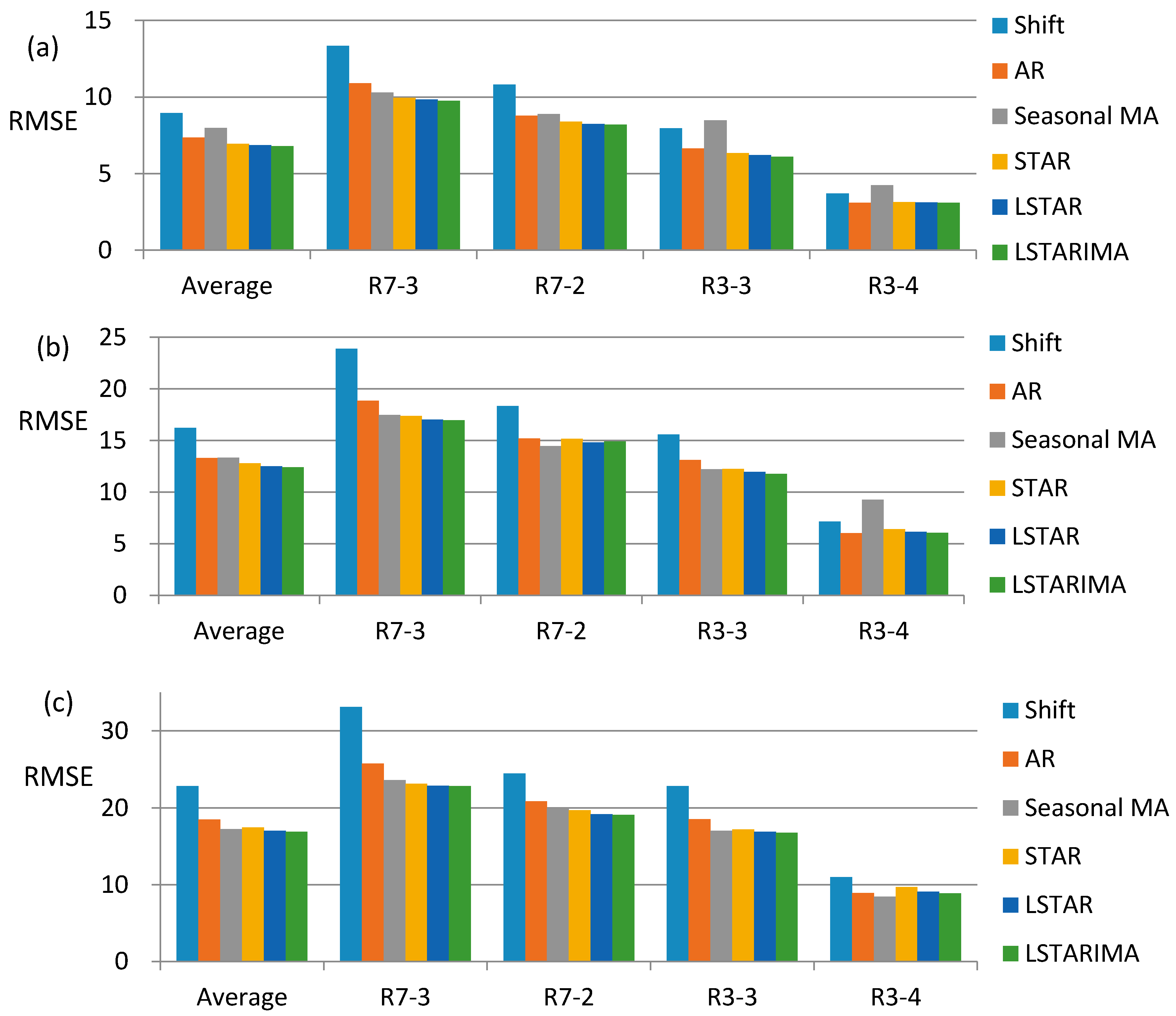
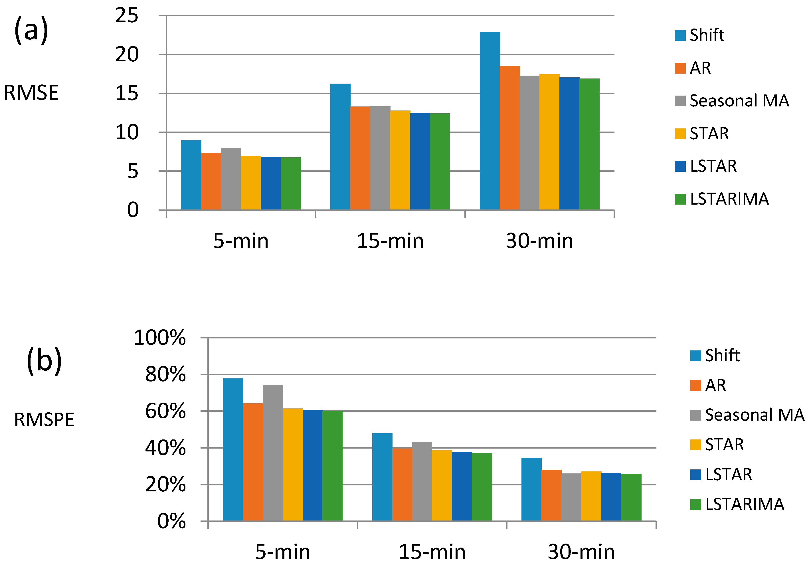
• Related simulations were performed. Through the simulation results, we observed that the prediction accuracy of LSTAR was a bit lower than the LSTARIMA model. However, the computational complexity of the LSTAR model was also lower than the LSTARIMA model. Therefore, there existed a tradeoff between the prediction accuracy and the computational complexity for the two models.

The rest of this paper is organized as follows. In Section 2, state-of-the-art traffic information collection, traffic prediction, and traffic applications are reviewed. In Section 3, we introduce the LSTAR model, the construction of the weight matrix of the LSTAR model, and a new traffic information collection method. In Section 4, parameters estimation methods of the LSTAR model are given and proven. In Section 5, the experimental evaluation is presented. Finally, Section 6 provides the conclusions and identifies future research directions.

2. State-of-the-Art and Related Topics

Traffic information collection provides the data input for traffic prediction, and there are many applications that use traffic prediction results to improve traffic conditions. In this section, the state-of-the-art traffic information collection, traffic prediction, and urban traffic applications are reviewed.

2.1. Traffic Information Collection

As traffic information is the base data of ITS, how to collect traffic information efficiently is an important area of research. Loop detectors are pressure, magnetic, and other sensors buried underground to detect if there are vehicles passing over them. They are widely deployed in urban areas to count the number of vehicles passing through fixed points of roads. Compared to loop detector technology, machine-vision-based traffic monitoring is a state-of-the-art approach with the advantages of easy maintenance, real-time visualization, and high flexibility [14]. With properly installed cameras, traffic information such as speed, volume, and even traffic accidents can be detected. However, it is expensive to establish these systems as well as to maintain a huge number of fixed devices on the road side, and they can only gather the traffic information of fixed points.

With the equipment of global position system (GPS) receivers on vehicles or mobile phones, vehicles can detect their own real-time location and speed. An alternative traffic information collection approach has been proposed to estimate the traffic state by checking the location and speed of some vehicles running on the road [15,16]. These probe vehicles are known as floating vehicles, and are normally buses and taxis. Due to the low cost of GPS receivers, the overall cost of the floating vehicles system is low. The shortcoming of floating vehicles is that their distribution in the urban traffic network is not even in space and time, which means that they may not be able to provide complete traffic states of the whole road network.

Vehicular Ad hoc Networks (VANET) [17,18,19] are an emerging technology developed for traffic security and data transformation [20]. In recent years, many research studies have used VANET to collect traffic information. The first type of system uses VANET to only estimate the traffic density of the road by detecting the number of vehicles in the VANET communication range [21]. The other type of system assumes that each vehicle is also equipped with a GPS receiver so more detailed traffic information can be collected [22,23]. As GPS receivers are more commonly equipped when compared with VANET and GPS can provide more information, more research has focused on the approach with GPS. With the communication capability of VANET, the collected traffic information can be easily shared and used by other ITS applications such as traffic prediction, route planning, and so on.

After traffic information is collected, it can be used as an input to other ITS applications as base data. Since VANET can obtain the traffic information of the whole network without infrastructure and can be easily integrated with other ITS systems, it was used to collect traffic information in our paper. Section 3.3 discussed our traffic information collection method via VANET in detail.

2.2. Traffic Prediction

Short-term traffic prediction is one of the most important topics in ITS research and practice. Aside from the ARIMA series prediction method, there have also been many other methodologies engaged for this purpose.

The Kalman filtering method [24,25], which is based on historical data and present data to predict a future state, has been widely used in the forecasting of traffic flow. However, its computational complexity is too high for complex urban traffic flow prediction. Neural Networks (NNs) models [26,27] have also been utilized to predict traffic flow for their high prediction accuracy. The weak point of NNs is the long model training time. Other research studies have referred to Support Vector Machines (SVM) [28]. However, the error of SVM is high under the circumstance of peak periods and blocking traffic accidents compared with the Bayesian network [29].

The K-NN method (K-nearest neighborhood) [30] performs well in short-term forecasting even when accidents have occurred. However, this algorithm has high complexity and needs a large amount of calculation when searching for class neighbors. Markov-based models [31] have also shown good performance on traffic flow prediction since the traffic condition at the next interval is closely related to the recent states. However, in these models, there are many states to consider. New technologies such as big data [32] and particle filtering [33,34] have also been used in traffic predication and other urban mobility applications.

Although these traffic prediction approaches have provided good prediction results in some scenarios, most of them are too complex or require a long training time. Thus, there have been respectable efforts put towards improving various ARIMA prediction models.

2.3. Urban Traffic Applications

Current traffic information and predicted traffic information are the base data of ITS, but they are meaningless without practical applications. Route planning and vehicle navigation systems are some of the most popular applications that use real-time and predicted traffic information [35]. The first-generation route planning system only considers the static features of the road network to obtain the shortest path. With the development of real-time traffic information collection technology, dynamic route planning has been proposed to re-calculate the new shortest path with the updated real-time data at each intersection. Such a system provides better travel planning when compared with the static route. However, using only current data may lead to frequent route changes in complex traffic conditions. The newest route planning systems use the predicted traffic information to arrive at the best and most stable route to the destination.

The other main applications using current and predicted traffic information are traffic management applications. The most common usage is to display current traffic states, the predicted traveling time to land mark locations, and traveling proposals on the traffic information board. With this information, drivers can re-plan their travel accordingly. Adaptive traffic signal control is the key technology of traffic management. The reactive traffic signaling control system adjusts the signal phase and cycle lengths according to current traffic data. The predictive traffic signal systems retime the traffic sign according to the predicted traffic information. With the predictive approach, the total waiting time of vehicles is reduced and the efficiency of the traffic network is improved [36].

Predicted traffic information is not only used by navigation systems and traffic management systems, but also by other urban applications such as parking management and so on. For the wide usage of traffic prediction, there are continuous research interests in this field.

3. Model and Preliminaries

3.1. LSTAR Model Construction

According to the STARIMA model defined in Reference [11], both space and time are considered.

$$Z_t={{\displaystyle \sum }}_{k=1}^p{{\displaystyle \sum }}_{l=0}^{{\lambda }_k}{\varphi }_{kl}{W}_l{z}_{t-k}-{{\displaystyle \sum }}_{k=1}^q{{\displaystyle \sum }}_{l=0}^{m_k}{\theta }_{kl}{W}_l{\epsilon }_{t-k}+{\epsilon }_t.$$

(1)

$Z_t$ is an N-dimensional column vector of road i, while i = 1, 2,…, N, and $W_l$ is an $N\times N$ matrix with element $w_{ij}^l$. ${\epsilon }_t$ is the residual vector. ${\varphi }_{kl}$, ${\theta }_{kl}$ are the AR and MA parameters, respectively.

Then, the observation of road $i$, $z_i\left(t\right)$ can be described as:

$$z_i\left(t\right)={\displaystyle \sum }_{k=1}^p{\displaystyle \sum }_{l=0}^{{\lambda }_k}{\displaystyle \sum }_{j=1}^N{\varphi }_{kl}{w}_{ij}^{\left(l\right)}{z}_j\left(t-k\right)-{\displaystyle \sum }_{k=1}^q{\displaystyle \sum }_{l=0}^{m_k}{\displaystyle \sum }_{j=1}^N{\theta }_{kl}{w}_{ij}^{\left(l\right)}{\epsilon }_j\left(t-k\right)+{\epsilon }_i\left(t\right).$$

(2)

In 2014, a new space-time model, the localized STARIMA (LSTARIMA) model, was proposed by Cheng et al. [13] to consider spatial heterogeneity and temporal non-stationarity. The model is described by the following form:

$$Z_i\left(t\right)={\displaystyle \sum }_{k=1}^{p_i}{\displaystyle \sum }_{h=0}^{{\lambda }_k\left(t-k,i\right)}{\varphi }_{i,kh}{W}^{\left(h,t-k,i\right)}{Z}_i\left(t-k\right)-{\displaystyle \sum }_{l=1}^{q_i}{\displaystyle \sum }_{h=0}^{n_l\left(t-l,i\right)}{\theta }_{i,lh}{W}^{\left(h,t-l,i\right)}{\epsilon }_i\left(t-l\right)+{\epsilon }_i\left(t\right).$$

(3)

$Z_i\left(t\right)$ is an N-dimensional column vector of the observation value on link 1, …, N with tag $i$ at time $t$, which can be any prediction variable of roads such as speed, traffic flow, density, and so on. The term ${\epsilon }_i\left(t\right)$ is a residual on link 1, …, N at time $t$. The first term in Equation (3) is the AR component, whereas the second term is the MA. The parameters $p_i$ and $q_i$ are the AR and MA orders, respectively. $h$ is the spatial order that represents the order of spatial separation between two locations. The parameters ${\lambda }_k\left(t-k,i\right)$ and $n_l\left(t-l,i\right)$ are the dynamic spatial orders associated with the $k\mathrm{th}$ and $l\mathrm{th}$ temporally lagged terms in the AR and MA components, respectively. They specify the size of the spatial neighborhood that could influence the link of interest $i$ within temporal lags $k$ and $l$. The parameters $W^{\left(h,t–k,i\right)}$ and $W^{\left(h,t–l,i\right)}$ are the dynamic spatial weight matrices $W^{\left(h,t,i\right)}$ pertaining to link $i$ at temporal lags $k$ and $l$. ${\varphi }_{i,kh}$ and ${\theta }_{i,lh}$ are the AR and MA parameters for each link $i \left(i=1, 2, \dots , N\right).$

Although spatial tag $i$ was added to $Z_i\left(t\right)$ in the LSTARIMA model construction, the spatial heterogeneity was not fully considered. As the $Z_i\left(t\right)$ here is an N-dimension column vector which covers all of the roads (road 1, 2, …, N) in the network, all of the roads will share the same ${\varphi }_{i,kh}$ and ${\theta }_{i,lh}$. In this LSTARIMA model, the same matrix W is used for both AR and MA components. As the weight matrix of AR and MA components is not always the same, using only one weight matrix $W$ is not proper.

In this paper, different weight matrices $W$, $U$ were used for AR and MA components and individual road traffic flow observation $z_i\left(t\right)$, according to Equation (2), was defined to allow every road to have its own weight matrix $W_i$, $U_i$ according to spatial location, but not sharing the same weight matrix among all roads, as in Equation (3).

Then, the LSTARIMA can be rewritten as follows:

$$z_i\left(t\right)={\displaystyle \sum }_{k=1}^{p_i}{\displaystyle \sum }_{h=0}^{{\lambda }_{i,k}}{\displaystyle \sum }_{j=1}^{N_i}{\varphi }_{i,kh}{w}_{ij}^{\left(h\right)}\left(t-k\right)z_j\left(t-k\right)-{\displaystyle \sum }_{k=1}^{q_i}{\displaystyle \sum }_{h=0}^{m_{i,k}}{\displaystyle \sum }_{j=1}^{N_i}{\theta }_{i,kh}{u}_{ij}^{\left(h\right)}\left(t-k\right){\epsilon }_j\left(t-k\right)+{\epsilon }_i\left(t\right).$$

(4)

The parameters $w_{ij}^{\left(h\right)}\left(t-k\right)$ and $u_{ij}^{\left(h\right)}\left(t-l\right)$ are the elements of dynamic spatial weight matrices $W_i^{\left(h\right)}\left(t-k\right)$ and $U_i^{\left(h\right)}\left(t-l\right)$ pertaining to link $i$ at temporal lags $k$ and $l$. Like the traditional STARIMA model, LSTARIMA makes use of spatial weight matrices $W$ and $U$ to model the influence of the spatiotemporal neighborhoods. However, it relaxes the globally fixed temporal dependence for all locations by using different AR and MA parameters according to location. Furthermore, it accounts for the temporal non-stationarity by allowing the matrix elements value and size of the spatial neighborhoods to vary with time.

According to Bo [37], the ARMA model can be properly approximated by the high-order AR model. As AR only has one type of parameter to be estimated, ARMA and ARIMA have two or three types of parameters to be estimated, and the parameters estimation of AR is easy even when the order is a little bit higher. There exist plenty of studies that have used a high-order AR model to approximate many processes of interest [37]. Furthermore, traffic flow has complex dynamics and may not exactly match an ARIMA model. In addition, many studies have removed MA and used only different AR models to conduct traffic prediction and obtain good results with limited AR order [38]. For reducing computational complexity and real-time prediction purpose, in this paper, we proposed the LSTAR model for traffic flow prediction.

With the MA component removed, the LSTARIMA prediction model (Equation (4)) is changed into the following LSTAR model:

$$z_i\left(t\right)={\displaystyle \sum }_{k=1}^{p_i}{\displaystyle \sum }_{h=0}^{{\lambda }_{i,k}}{\displaystyle \sum }_{j=1}^{N_i}{\varphi }_{i,kh}{w}_{ij}^{\left(h\right)}\left(t-k\right)z_j\left(t-k\right)+{\epsilon }_i\left(t\right)$$

(5)

where ${\mathsf{\epsilon }}_i\left(t\right)$ is white noise, ${\varphi }_{i,hk}$ is the parameter for each link $i \left(i=1, 2, \dots , N\right)$, and $w_{ij}^{\left(h\right)}\left(t-k\right)$ are the elements of the dynamic spatial weight matrix $W_i^{\left(h\right)}\left(t-k\right)$ pertaining to link $i$ at temporal lag $k$.

3.2. Weight Matrix Construction

Weight matrix construction is an essential topic in STARIMA models. In the STARIMA model, the weight matrix is time invariant and equal for the same neighbor order. In the LSTARIMA model, a time variant weight matrix was introduced to improve traffic prediction accuracy with lower AR and MA orders. Furthermore, the speed difference was used to construct the weight matrix in the LSTARIMA model [13]. The speed of a road is an important character of traffic flow, but is not the essential one in terms of impact to surrounding roads. It is obvious that a road that outputs only one vehicle will not impact neighbor roads at the same level as saturated roads with the same speed. The traffic output amount to the neighbor roads in a time slot has more impact on the future traffic state of neighbor roads. Thus, the output vehicle number during a time slot was used in the weight matrix construction instead of speed in this paper.

For all pairwise road sections $\left(i,j\right)$ with spatial lag $h$, the corresponding $w_{ij}^{\left(h\right)}\left(t\right)$ is defined as follows:

$$w_{ij}^{(h)}(t)=\{\begin{array}{cc}1& h=0,i=j\hfill \\ \frac{Q_{ij}(t)}{\sum Q(t)}& h=1,\sum Q(t)\ne 0\hfill \\ \frac{Q^{(h)}{}_{ij}(t)}{\sum Q^{(h)}(t)}& h\ne 1,\sum Q^{(h)}(t)\ne 0\hfill \\ 0& \sum Q^{(h)}(t)=0\hfill \end{array}$$

(6)

where $Q_{ij}\left(t\right)$ is the number of vehicles running from road $j$ towards road $i$ at time slot $t$ and $\sum Q\left(t\right)$ is the sum of vehicle numbers from directly connected roads to road $i$ at time slot $t$. $Q^{\left(h\right)}{}_{ij}\left(t\right)$ is the number of vehicles on the $h$ order neighbor road $j$ towards $h-1$ order neighbor of road $i$ at time slot $t$, and $Q^{\left(h\right)}{}_{ij}\left(t\right)$ = 0 if $j$ is not the $h$ order neighbor of $i$. $\sum Q^{\left(h\right)}\left(t\right)$ is the sum of $Q^{\left(h\right)}{}_{ij}\left(t\right)$.

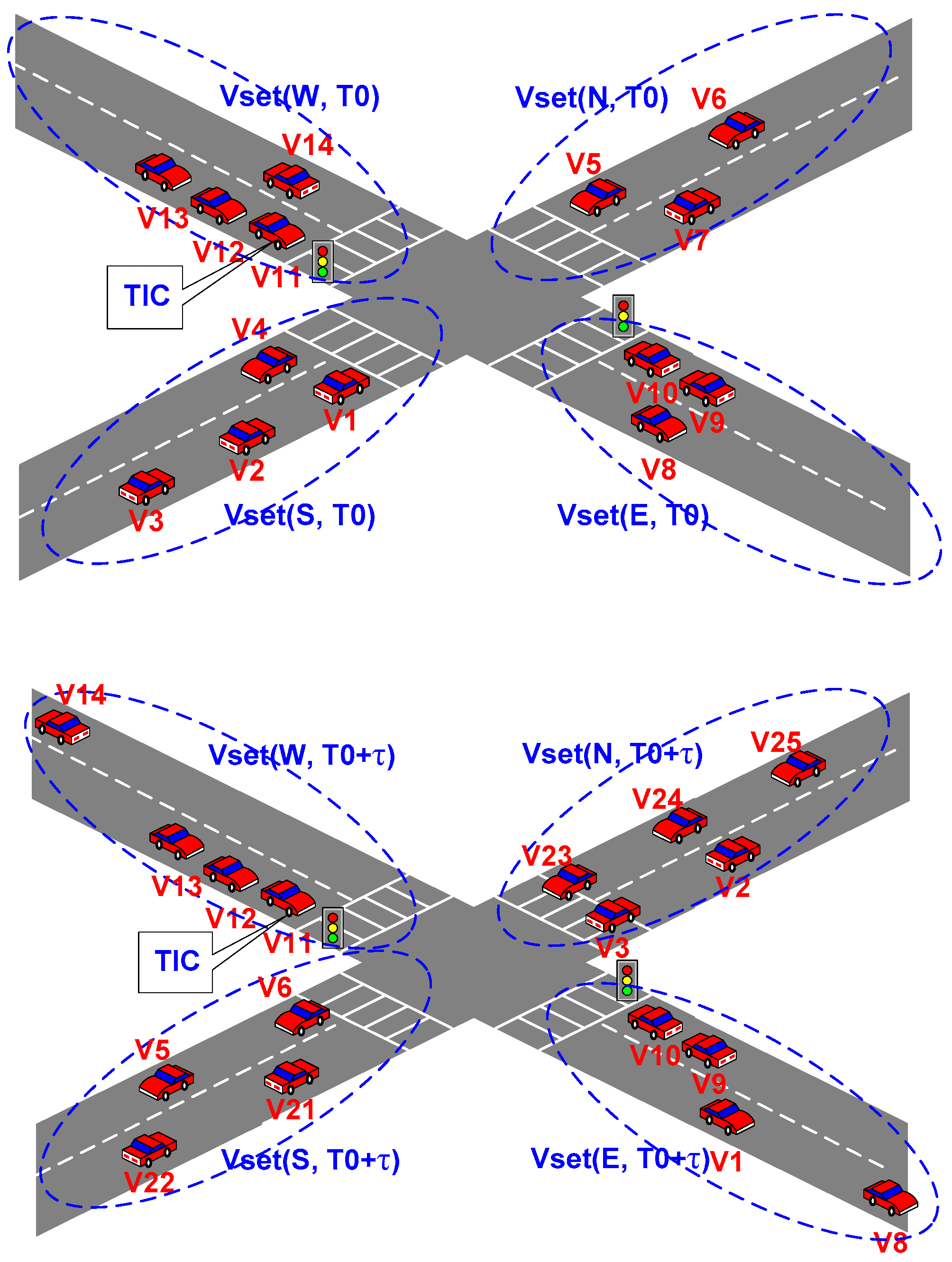
3.3. Traffic Information Collection

In this paper, we proposed a traffic information collection system via VANET for urban areas. In this system, each vehicle was assumed to have a GPS receiver and VANET equipped to report its location. This assumption is reasonable as currently more and more vehicles are equipped with such devices. Considering that there are always traffic lights at the intersection of urban roads, we used vehicles stopped at red lights to collect traffic information by checking the location of all vehicles inside their VANET communication range periodically.

As shown in Figure 1, when the traffic light turned red for the east-west direction, the first vehicle stopped at the west side was selected as the traffic information collector (TIC). If there were no vehicle stops at the west side, the first vehicle stopped at the east side would be the TIC. In the example of Figure 1, vehicle V11 is the TIC and collects the traffic information during the red light period.

Figure 1. Traffic information collection.

Step 1.

When the traffic light turns to red at T0, V11 broadcasts traffic information collection request.

Step 2.

All of the vehicles in the communication range $R$ of V11 will report their locations to V11 after receiving the request from V11.

Step 3.

V11 catalogs the vehicles to four vehicle sets according to the location. They are marked as $Vset\left(E, T0\right)$, $Vset\left(S, T0\right)$, $Vset\left(W, T0\right)$, and $Vset\left(N, T0\right)$.

Step 4.

After time $\tau <R/V_{max}$, V11 collects the traffic information again according to Steps 1–3 and obtains $Vset\left(E, T0+\tau \right)$, $Vset\left(S, T0+\tau \right)$, $Vset\left(W, T0+\tau \right)$, $Vset\left(N, T0+\tau \right)$. $V_{max}$ is the maximum allowed velocity. Time $\tau <R/V_{max}$ will let all vehicles running towards the intersection be detectable at time $T0+\tau$.

For example:

If R = 150 m and $V_{max}=20\mathrm{m}/\mathrm{s}$, $\tau$ = 5 s can be used as $5<\frac{150}{20}=7.5$. The maximal length a vehicle can run during $\tau$ is $\frac{20\mathrm{m}}{\mathrm{s}}\times 5\mathrm{s}=100\mathrm{m}<150\mathrm{m}$. Then, no vehicle entering the intersection at T0 can run outside the communication range of V11 and be detectable at $T0+\tau$.

Step 5.

The vehicles’ set run from road A to road B is calculated by formula: $Vset\left(A\to B, T0+\tau \right)=Vset\left(A, T0\right)\cap Vset\left(B, T0+\tau \right)$.

For example:

As shown in Figure 1, the traffic output from S to E from T0 to $T0+\tau$ is:

$$\begin{gathered} Vset\left(S\to E, T0+\tau \right)=Vset\left(S, T0\right)\cap Vset\left(E, T0+\tau \right) \\ =\left\{V1,V2,V3,V4\right\}\cap \left\{V1,V8,V9,V10\right\}=\left\{V1\right\} \end{gathered}$$

Step 6.

The TIC calculates the traffic output of each road with time interval $\tau$ until the traffic light for the east-west direction turns green. As the traffic light for the south-north direction turns red, the first vehicle stopped at the north or south side will be selected as the TIC and collect traffic information continuously.

As a part of the advance travel information system (ATIS), the TIC will send out the collected traffic information via VANET for applications such as traffic prediction. In normal urban traffic conditions, there should always be vehicles stopped at the red light to act as the TIC. If there is no vehicle stopped at the red light to be the TIC, the traffic information of the last time slot will be used. This is acceptable as it normally happens in very low traffic density cases and real-time traffic information is not important.

With the collected traffic information, the traffic output of each road section j can be calculated by:

$$Q^{\left(h\right)}{}_{ij}\left(t\right)={\displaystyle \sum }_n{\displaystyle \sum }_{m}Vset\left(j\to j_m,T+n\mathsf{\tau }\right),$$

where $T+n\mathsf{\tau }\in \left(t-1,t\right]$, $j$ is the $h$ order neighbor of road $i$, $j_m$ is the $h-1$ order neighbor of road $i$ ($j_m$ is $i$ when $h=1$), $m$ is the total number of $j_m$ which are downstream $j$.

4. Main Results

For the LSTAR model, in this section we discuss how to determine the parameter ${\varphi }_{i,kh}$ with a given weight matrix $W_i^{\left(h\right)}\left(t\right)$. With the determined weight matrix $W_i^{\left(h\right)}\left(t\right)$ and ${\varphi }_{i,kh}$, the future traffic observation $\widehat{z}\left(t\right)$ of road $i$ can be predicted. Normally, $w_{ij}^{\left(h\right)}\left(t\right)$ is time variant. When the traffic flow distribution is stable in the road network, $w_{ij}^{\left(h\right)}\left(t\right)$ will be time invariant since $\frac{Q^{\left(h\right)}{}_{ij}\left(t\right)}{\sum Q^{\left(h\right)}\left(t\right)}$ is constant. Considering the weight matrix differences of being time invariant or not, two theorems are discussed, and the LSTAR parameters estimation can be conducted accordingly.

Definitions 1.

$r_{ij}\left(m\right)$ is the correlation coefficient of road $i$ and $j$, $r_i\left(m\right)=r_{ii}\left(m\right)$ is the autocorrelation coefficient of road $i$. We define ${\Phi }_i={\left[{\varphi }_{i,10},{\varphi }_{i,11},\dots {\varphi }_{i,1{\lambda }_{i,0}},{\varphi }_{i,20},{\varphi }_{i,21},\dots ,{\varphi }_{i,p_i{\lambda }_{i,k}}\right]}^T$, let $n={{\displaystyle \sum }}_{k=1}^{p_i}{\lambda }_{i,k}$ to be the dimension of ${\Phi }_i$. $R_i={\left[r_i\left(0\right),r_i\left(1\right),\dots ,r_i\left(n-1\right)\right]}^T, \Sigma ={\left[{\sigma }_i{}^2,0,\dots ,0\right]}^T, S\left(h,m\right)={{\displaystyle \sum }}_{j=1}^{N_i}{w}_{ij}^{\left(h\right)}{r}_{ij}\left(m\right)$,

$$A=\left[\begin{array}{cccc}S\left(0,1\right)& S\left(1,1\right)& \cdots & S\left({\lambda }_{i,k},p_i\right)\\ S\left(0,0\right)& S\left(1,0\right)& \cdots & S\left({\lambda }_{i,k},p_i-1\right)\\ S\left(0,1\right)& S\left(1,1\right)& \cdots & S\left({\lambda }_{i,k},p_i-2\right)\\ ⋮& ⋮& ⋮& ⋮\\ S\left(0,n-1\right)& S\left(1,n-1\right)& \cdots & S\left({\lambda }_{i,k},n-1-p_i\right)\end{array}\right],\overline{A}=\left[\begin{array}{cc}A& R_i-\Sigma \end{array}\right].$$

Theorem 1 follows:

Theorem 1.

If $W_i^{\left(h\right)}\left(t\right)$ is time invariant and $Rank\left(A\right)=Rank\left(\overline{A}\right)=n$, the LSTAR model can be uniquely determined.

Proof. 

As $W_i^{\left(h\right)}\left(t\right)$ is time invariant, we can observe that $W_i^{\left(h\right)}\left(t\right)=W_i^{\left(h\right)}\left(t-k\right)$ and it can be rewritten to $W_i^{\left(h\right)}$.

The model of Equation (5) will be a time invariant system. Since $z_i\left(t\right)$ is a stationary random signal, Equation (5) will be:

$$z_i\left(t\right)={\displaystyle \sum }_{k=1}^{p_i}{\displaystyle \sum }_{h=0}^{{\lambda }_{i,k}}{\displaystyle \sum }_{j=1}^{N_i}{\varphi }_{i,kh}{w}_{ij}^{\left(h\right)}{z}_j\left(t-k\right)+{\epsilon }_i\left(t\right).$$

(7)

Pre-multiplying both sides of the model (Equation (7)) by $z_i\left(t-m\right)$:

$$z_i\left(t\right)z_i\left(t-m\right)={\displaystyle \sum }_{k=1}^{p_i}{\displaystyle \sum }_{h=0}^{{\lambda }_{i,k}}{\displaystyle \sum }_{j=1}^{N_i}{\varphi }_{i,kh}{w}_{ij}^{\left(h\right)}{z}_j\left(t-k\right)z_i\left(t-m\right)+{\epsilon }_i\left(t\right)z_i\left(t-m\right).$$

(8)

Taking the expected values in both sides, we obtain an equation similar to the Yule-Walker equation:

$$r_i\left(m\right)={\displaystyle \sum }_{k=1}^{p_i}{\displaystyle \sum }_{h=0}^{{\lambda }_{i,k}}{\displaystyle \sum }_{j=1}^{N_i}{\varphi }_{i,kh}{w}_{ij}^{\left(h\right)}{r}_{ij}\left(m-k\right)+{\sigma }_i{}^2\delta \left(m\right)$$

(9)

where the expected value is:

$$E({\epsilon }_i\left(t\right)z_i\left(t-m\right))={\sigma }_i{}^2\delta \left(m\right).$$

(10)

As ${\varphi }_{i,hk}$ does not have tag j, we obtain:

$$r_i\left(m\right)={\displaystyle \sum }_{k=1}^{p_i}{\displaystyle \sum }_{h=0}^{{\lambda }_{i,k}}{\varphi }_{i,kh}{\displaystyle \sum }_{j=1}^{N_i}{w}_{ij}^{\left(h\right)}{r}_{ij}\left(m-k\right)+{\sigma }_i{}^2\delta \left(m\right).$$

(11)

For Equation (11), rewrite ${\varphi }_{i,kh}$ to a column vector as ${\Phi }_i={\left[{\varphi }_{i,10},{\varphi }_{i,11},\dots ,{\varphi }_{i,1{\lambda }_{i,0}},{\varphi }_{i,20},{\varphi }_{i,21},\dots {\varphi }_{i,k{\lambda }_{i,k}}\right]}^T$. In addition, $\mathrm{n}={{\displaystyle {\sum }_{\mathrm{k}=\mathrm{1}}^{{\mathrm{p}}_{\mathrm{i}}}\mathsf{\lambda }}}_{\mathrm{i},\mathrm{k}}$ is the number of parameters ${\varphi }_{i,kh}$ to be estimated.

As $S(h,m)={\displaystyle {\sum }_{j=1}^{N_i}{w}_{ij}^{(h)}}{r}_{i,j}(m)$, we obtain:

$$\left[\begin{array}{c}{r}_i(0)\\ r_i(1)\\ \begin{array}{c}{r}_i(2)\\ ⋮\\ r_i(n-1)\end{array}\end{array}\right]=\left[\begin{array}{cccc}S(0,1)& S(1,1)& \cdots & S({\lambda }_{i,k},p_i)\\ S(0,0)& S(1,0)& \cdots & S({\lambda }_{i,k},p_i-1)\\ S(0,1)& S(1,1)& \cdots & S({\lambda }_{i,k},p_i-2)\\ \begin{array}{c}⋮\\ S(0,n-1)\end{array}& \begin{array}{c}⋮\\ S(1,n-1)\end{array}& \begin{array}{c}⋮\\ \cdots \end{array}& \begin{array}{c}⋮\\ S({\lambda }_{i,k},n-1-p_i)\end{array}\end{array}\right]\left[\begin{array}{c}{\varphi }_{i,10}\\ {\varphi }_{i,11}\\ \begin{array}{c}{\varphi }_{i,12}\\ ⋮\\ {\varphi }_{i,k{\lambda }_{i,k}}\end{array}\end{array}\right]+\left[\begin{array}{c}{\sigma }_i{}^2\\ 0\\ \begin{array}{c}0\\ ⋮\\ 0\end{array}\end{array}\right].$$

(12)

Let $A=\left[\begin{array}{cccc}S\left(0,1\right)& S\left(1,1\right)& \cdots & S\left({\lambda }_{i,k},p_i\right)\\ S\left(0,0\right)& S\left(1,0\right)& \cdots & S\left({\lambda }_{i,k},p_i-1\right)\\ S\left(0,1\right)& S\left(1,1\right)& \cdots & S\left({\lambda }_{i,k},p_i-2\right)\\ ⋮& ⋮& ⋮& ⋮\\ S\left(0,n-1\right)& S\left(1,n-1\right)& \cdots & S\left({\lambda }_{i,k},n-1-p_i\right)\end{array}\right]$, $R_i=\left[\begin{array}{c}{r}_i\left(0\right)\\ \begin{array}{c}{r}_i\left(1\right)\\ r_i\left(2\right)\\ ⋮\end{array}\\ r_i\left(n-1\right)\end{array}\right]$, $\mathrm{\Sigma }=\left[\begin{array}{c}{\sigma }_i{}^2\\ \begin{array}{c}0\\ 0\\ ⋮\\ 0\end{array}\end{array}\right]$.

Then, the augmented matrix of Equation (12) is:

$$\overline{A}=\left[\begin{array}{ccccc}S\left(0,1\right)& S\left(1,1\right)& \cdots & S\left({\lambda }_{i,k},p_i\right)& r_i\left(0\right)-{\sigma }_i{}^2\\ S\left(0,0\right)& S\left(1,0\right)& \cdots & S\left({\lambda }_{i,k},p_i-1\right)& r_i\left(1\right)\\ S\left(0,1\right)& S\left(1,1\right)& \cdots & S\left({\lambda }_{i,k},p_i-2\right)& r_i\left(2\right)\\ ⋮& ⋮& ⋮& ⋮& ⋮\\ S\left(0,n-1\right)& S\left(1,n-1\right)& \cdots & S\left({\lambda }_{i,k},n-1-p_i\right)& r_i\left(n-1\right)\end{array}\right]=\left[\begin{array}{cc}A& R_i\end{array}-\mathrm{\Sigma }\right].$$

If $Rank\left(A\right)=n$, then $Rank\left(\overline{A}\right)=n$ and we will have a unique solution of parameters ${\Phi }_i$:

$${\Phi }_i=A^{-1}\left(R_i-\mathrm{\Sigma }\right)$$

(13)

Then, we can uniquely define the LSTAR model and predict traffic flow with it.

If $R\left(A\right)\ne R\left(\overline{A}\right)$, there is no solution for Equation (12).

If $Rank\left(A\right)=Rank\left(\overline{A}\right)<n$, there are infinite solutions for ${\Phi }_i$.☐

Remark 1.

In case the spatial weight matrix $W_i^{\left(h\right)}\left(t\right)$ is time invariant, we can determine the LSTAR prediction model by the correlation of roads. We can uniquely define the LSTAR model when $Rank\left(A\right)=Rank\left(\overline{A}\right)=n$. When $Rank\left(A\right)=Rank\left(\overline{A}\right)<n$, there will be many solutions for parameter $\Phi$ . This means that we have defined more parameters than are actually needed. We can reduce ${\lambda }_{i,k}$ and/or $p_i$ to obtain a unique LSTAR model.

Definitions 2.

Let $r_i^{\prime }\left(m\right)$ be the autocorrelation coefficient of $ith$ element of $U\left(t\right)=W\left(t\right)Z\left(t\right)$, where the matrix $W\left(t\right)={{\displaystyle \sum }}_{h=0}^{{\lambda }_{i,k}}{W}_i^{\left(h\right)}\left(t\right)$, which combines all spatial effect defined in $W_i^{\left(h\right)}\left(t\right)$ to one matrix, and $Z\left(t\right)={\left[z_1\left(t\right),z_2\left(t\right),\dots , z_{N_i}\left(t\right)\right]}^T$ is the vector form of $z_i\left(t\right)$. We define ${\Phi }_i={\left[{\varphi }_{i,1},{\varphi }_{i,2},\dots ,{\varphi }_{i,p_i}\right]}^T$, ${\overline{R}}_i^{\prime }={\left[{\overline{r}}_i^{\prime }\left(0\right),{\overline{r}}_i^{\prime }\left(1\right),\dots ,{\overline{r}}_i^{\prime }\left(p_i-1\right)\right]}^T$, $\Sigma ={\left[{\sigma }_i{}^2,0,\dots , 0\right]}^T$,

$$A^{\prime }=\left[\begin{array}{cccc}{r}_i^{\prime }\left(1\right)& r_i^{\prime }\left(2\right)& \cdots & r_i^{\prime }\left(p_i\right)\\ r_i^{\prime }\left(0\right)& r_i^{\prime }\left(1\right)& \cdots & r_i^{\prime }\left(p_i-1\right)\\ ⋮& ⋮& ⋮& ⋮\\ r_i^{\prime }\left(p_i-2\right)& r_i^{\prime }\left(p_i-3\right)& \cdots & r_i^{\prime }\left(1\right)\end{array}\right],\overline{A^{\prime }}=\left[\begin{array}{cc}{A}^{\prime }& {\overline{R}}_i^{\prime }-\Sigma \end{array}\right].$$

We then present Theorem 2.

Theorem 2.

If $W_i^{\left(h\right)}\left(t\right)$ is time variant, the combined weight matrix $W\left(t\right)$ is full ranked, and $Rank\left(A^{\prime }\right)=Rank\left(\overline{A^{\prime }}\right)=p_i$, the LSTAR model can be uniquely determined.

Proof. 

According to the weight matrix $W_i^{\left(h\right)}\left(t\right)$ construction in the LSTAR model, the element $w_{ij}^{\left(h\right)}\left(t\right)$ will always be zero when $i$, $j$ is not at spatial order $h$. We combine all of the ${\lambda }_{i,k}$ weight matrix into one weight matrix, $W\left(t\right)$ = ${{\displaystyle \sum }}_{h=0}^{{\lambda }_{i,k}}{W}_i^{\left(h\right)}\left(t\right)$. This simplification is reasonable as (1) time variant $w_{ij}\left(t\right)$ can somehow give an effect similar to spatial order $h$; and (2) $w_{ij}\left(t\right)$ is always equal to the only non-zero $w_{ij}^{\left(h\right)}\left(t\right)$:

$$w_{ij}\left(t\right)=0+0+\dots +w_{ij}^{\left(h\right)}\left(t\right)+\dots +0=w_{ij}^{\left(h\right)}\left(t\right)\mathrm{number}\mathrm{of}\mathrm{zero}\mathrm{is}{\lambda }_{i,k}-1$$

Considering the combined spatial weight matrix $W\left(t\right)={{\displaystyle \sum }}_{h=0}^{{\lambda }_{i,k}}{W}_i^{\left(h\right)}\left(t\right)$, $Z\left(t\right)={\left[z_1\left(t\right),z_2\left(t\right),\dots ,z_{N_i}\left(t\right)\right]}^T$ is an $N_i$ dimension column vector that includes all neighbor roads within the spatial order to be considered by road $i$, and $\Sigma ={\left[{\sigma }_i{}^2,0,\dots ,0\right]}^T$, we can obtain a matrix from the LSTAR model according to Equation (5).

$$Z\left(t\right)={\displaystyle \sum }_{k=1}^{p_i}{\varphi }_{i,k}W\left(t-k\right)Z\left(t-k\right)+\Sigma \left(t\right)$$

(14)

when the rank of $W\left(t\right)$ is $N_i$, Equation (14) can be rewritten as:

$${\left[W\left(t\right)\right]}^{-1}\left[W\left(t\right)Z\left(t\right)\right]={\displaystyle \sum }_{k=1}^{p_i}{\varphi }_{i,k}W\left(t-k\right)\mathrm{Z}\left(t-k\right)+\mathrm{\Sigma }\left(t\right).$$

(15)

Let $U\left(t\right)=\left[W\left(t\right)\mathrm{Z}\left(t\right)\right]$, we obtain:

$${\left[W\left(t\right)\right]}^{-1}U\left(t\right)={\displaystyle \sum }_{k=1}^{p_i}{\varphi }_{i,k}U\left(t-k\right)+\Sigma \left(t\right).$$

(16)

${[W_i^{\left(h\right)}\left(t\right)]}^{-1}$ can be treated as an instantaneous window to $U\left(t\right)$, so $U\left(t\right)$ is stationary in the short term. We have:

$$\overline{U}\left(t\right)={\displaystyle \sum }_{k=1}^{p_i}{\varphi }_{i,k}U\left(t-k\right)+\Sigma \left(t\right).$$

(17)

Let $u_i\left(t\right)$ be the element of $U\left(t\right)$, then:

$${\overline{u}}_i\left(t\right)={\displaystyle \sum }_{k=1}^{p_i}{\varphi }_{i,k}{u}_i\left(t-k\right)+{\epsilon }_i\left(t\right).$$

(18)

Pre-multiplying both sides of Equation (18) by $u_i\left(t-m\right)$:

$${\overline{u}}_i\left(t\right)u_i\left(t-m\right)={\displaystyle \sum }_{k=1}^{p_i}{\varphi }_{i,k}{u}_i\left(t-k\right)u_i\left(t-m\right)+{\epsilon }_i\left(t\right)u_i\left(t-m\right).$$

(19)

Taking expected values in both sides, we obtain:

$${\overline{r}}_i^{\prime }\left(m\right)={\displaystyle \sum }_{k=1}^{p_i}{\varphi }_{i,k}{r}_i^{\prime }\left(m-k\right)+{\sigma }_i{}^2\delta \left(m\right)$$

(20)

where the expected value $r_i^{\prime }\left(m\right)=E\left(u_i\left(t-m\right)u_i\left(t-k\right)\right)$, ${\overline{r}}_i^{\prime }\left(m\right)=E({[W_i^{\left(h\right)}\left(t\right)]}^{-1}{u}_i\left(t\right)u_i\left(t-m\right))$, $E\left({\epsilon }_i\left(t\right)u_i\left(t-m\right)\right)={\sigma }_i{}^2\delta \left(m\right).$

We can then obtain:

$$\left[\begin{array}{c}{\overline{r}}_i^{\prime }\left(0\right)\\ \begin{array}{c}{\overline{r}}_i^{\prime }\left(1\right)\\ ⋮\end{array}\\ {\overline{r}}_i^{\prime }\left(p_i-1\right)\end{array}\right]=\left[\begin{array}{cccc}{r}_i^{\prime }\left(1\right)& r_i^{\prime }\left(2\right)& \cdots & r_i^{\prime }\left(p_i\right)\\ r_i^{\prime }\left(0\right)& r_i^{\prime }\left(1\right)& \cdots & r_i^{\prime }\left(p_i-1\right)\\ ⋮& ⋮& ⋮& ⋮\\ r_i^{\prime }\left(p_i-2\right)& r_i^{\prime }\left(p_i-3\right)& \cdots & r_i^{\prime }\left(1\right)\end{array}\right]\left[\begin{array}{c}{\varphi }_{i,1}\\ {\varphi }_{i,2}\\ \begin{array}{c}⋮\\ {\varphi }_{i,p_i}\end{array}\end{array}\right]+\left[\begin{array}{c}{\sigma }_i{}^2\\ \begin{array}{c}0\\ ⋮\\ 0\end{array}\end{array}\right]$$

(21)

Let ${\Phi }_i=\left[\begin{array}{c}{\varphi }_{i,1}\\ {\varphi }_{i,2}\\ \begin{array}{c}⋮\\ {\varphi }_{i,p_i}\end{array}\end{array}\right]$, $A^{\prime }=\left[\begin{array}{cccc}{r}_i^{\prime }\left(1\right)& r_i^{\prime }\left(2\right)& \cdots & r_i^{\prime }\left(p_i\right)\\ r_i^{\prime }\left(0\right)& r_i^{\prime }\left(1\right)& \cdots & r_i^{\prime }\left(p_i-1\right)\\ ⋮& ⋮& ⋮& ⋮\\ r_i^{\prime }\left(p_i-2\right)& r_i^{\prime }\left(p_i-3\right)& \cdots & r_i^{\prime }\left(1\right)\end{array}\right]$, ${\overline{R}}_i^{\prime }=\left[\begin{array}{c}{\overline{r}}_i^{\prime }\left(0\right)\\ \begin{array}{c}{\overline{r}}_i^{\prime }\left(1\right)\\ ⋮\end{array}\\ {\overline{r}}_i^{\prime }\left(p_i-1\right)\end{array}\right]$, $\mathrm{\Sigma }=\left[\begin{array}{c}{\sigma }_i{}^2\\ \begin{array}{c}0\\ ⋮\\ 0\end{array}\end{array}\right]$.

Then the augmented matrix of Equation (21) is:

$$\overline{A^{\prime }}=\left[\begin{array}{ccccc}{r}_i^{\prime }\left(1\right)& r_i^{\prime }\left(2\right)& \cdots & r_i^{\prime }\left(p_i\right)& {\overline{r}}_i^{\prime }\left(0\right)-{\sigma }_i{}^2\\ r_i^{\prime }\left(0\right)& r_i^{\prime }\left(1\right)& \cdots & r_i^{\prime }\left(p_i-1\right)& {\overline{r}}_i^{\prime }\left(1\right)\\ ⋮& ⋮& ⋮& ⋮& ⋮\\ r_i^{\prime }\left(p_i-2\right)& r_i^{\prime }\left(p_i-3\right)& \cdots & r_i^{\prime }\left(1\right)& {\overline{r}}_i^{\prime }\left(p_i-1\right)\end{array}\right]=\left[\begin{array}{cc}{A}^{\prime }& {\overline{R}}_i^{\prime }-\mathrm{\Sigma }\end{array}\right].$$

If $Rank\left(A^{\prime }\right)=p_i$, then $Rank\left(\overline{A^{\prime }}\right)=p_i$ and we will have a unique solution of parameters $\Phi$:

$${\Phi }_i={\left[A^{\prime }\right]}^{-1}({\overline{R}}_i^{\prime }-\mathrm{\Sigma }).$$

(22)

If $R\left(A^{\prime }\right)\ne R\left(\overline{A^{\prime }}\right)$, there is no solution for Equation (21).

If $Rank\left(A^{\prime }\right)=Rank\left(\overline{A^{\prime }}\right)<p_i$, there are infinite solutions for $\Phi$. ☐

Remark 2.

Unlike $W_i^{\left(h\right)}\left(t\right)$ with most of its elements being zero and normally not being full ranked, most elements of the combined weight matrix $W\left(t\right)$ are not zero. So $W\left(t\right)$ is normally a full rank matrix. For some special cases when $W\left(t\right)$ is not a full rank matrix, we can reduce the size of $W\left(t\right)$ to make it fully ranked. When $W\left(t\right)$ is a full rank matrix, we can uniquely define the LSTAR model when $Rank\left(A\right)=Rank\left(\overline{A}\right)=n$. Similar to Remark 1, we can reduce $p_i$ to obtain a unique LSTAR model if $Rank\left(A\right)=Rank\left(\overline{A}\right)<n$.

In this section, two theorems were given and proven according to the weight matrix determined. When the traffic flow distribution is stable, $W_i^{\left(h\right)}\left(t\right)$ can be treated as time invariant and Theorem 1 can be used. When the traffic flow distribution is not stable, $W_i^{\left(h\right)}\left(t\right)$ is time variant and Theorem 2 should be used. With the measured weight matrix $W_i^{\left(h\right)}\left(t\right)$ and estimated ${\Phi }_i$, future traffic state ${\widehat{z}}_i\left(t+1\right)$ can be predicted according to the LSTAR model (Equation (5)) by one-time slot shifting.

5. Practical Example and Experimental Evaluation

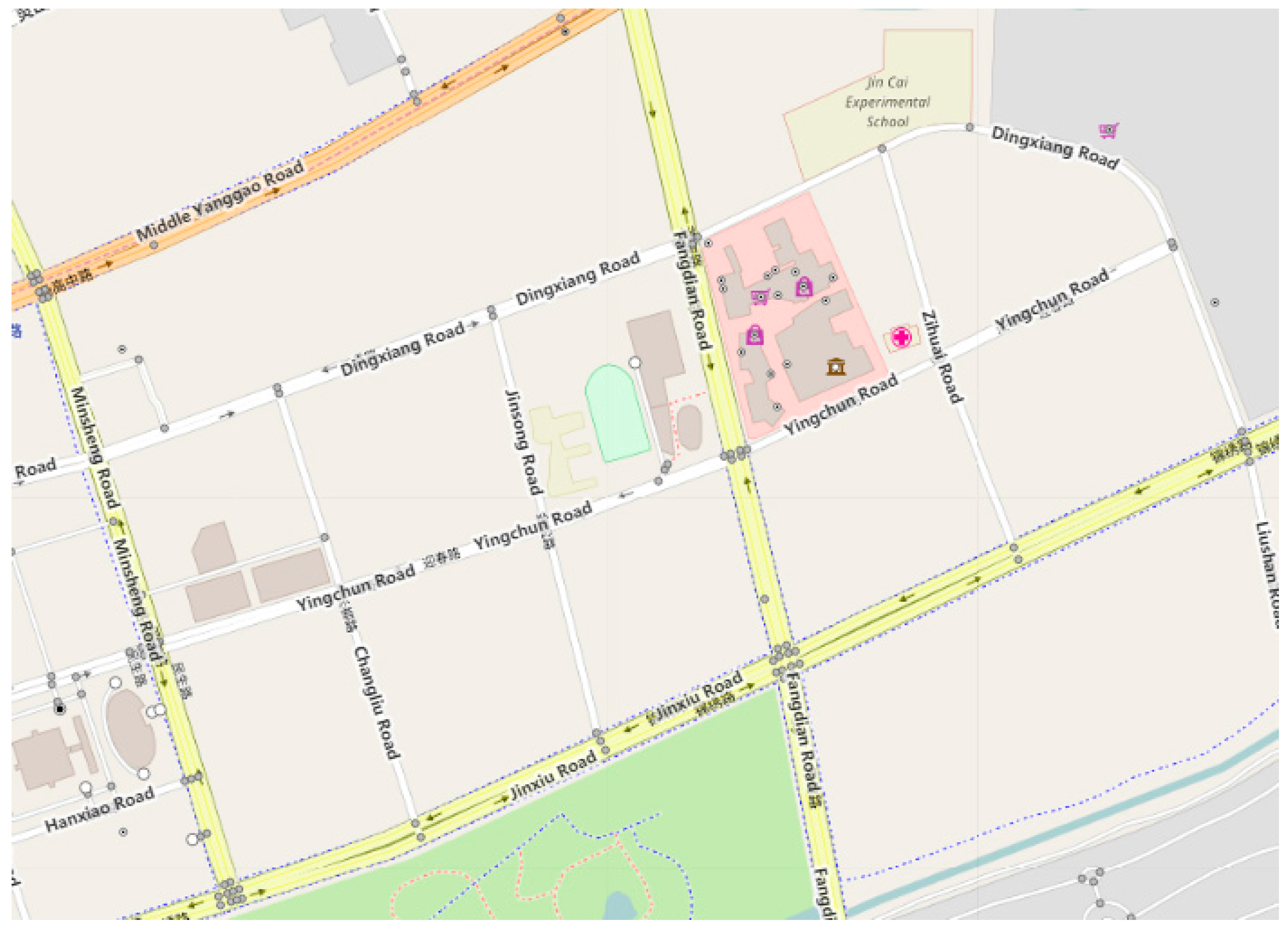
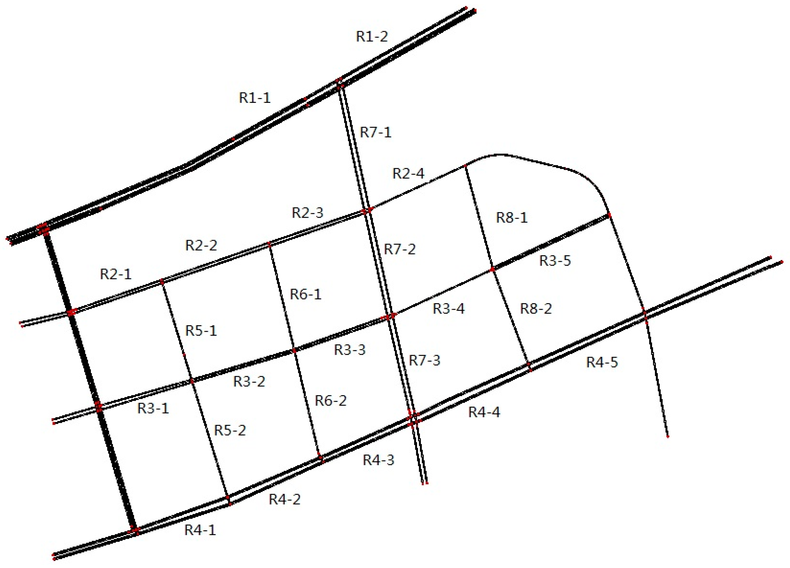
5.1. Practical Example

In this paper, we provide a practical example on how to use our LSTAR model to predict future traffic flow of the Shanghai Century Park area. To evaluate the prediction approach of LSTAR, we adopted the widely used traffic simulation tools Simulation of Urban Mobility (SUMO) [39] and OpenStreetMap (OSM) [40], which are recognized as promising candidates for traffic simulations, and the simulation results are commonly accepted as a replacement of real data. Additionally, plenty of works exist that have adopted SUMO and OSM as tools to generate traffic data for research [41,42].

In this example, we demonstrate the model-building procedure for our proposed LSTAR model in the context of traffic flow prediction on a road network. First, we downloaded the OSM format road network map of the area near Shanghai Century Park, as shown in Figure 2. The OSM format map not only included the geography topology of the road network, but also the road type, lane number, speed limitation, traffic light duration, and so on, according to real-world information. Then, the SUMO NetConvert tool was used to convert the OSM format map to a SUMO format map. SUMO was then used to simulate the traffic flow of this area according to the road network information converted from the OSM map.

Figure 2. OpenStreetMap (OSM) map of Shanghai Century Park area.

In the simulation, trip demands were generated randomly every two seconds according to the edge length. The “Fringe factor” was set to 4, which means that roads with no successor or no predecessor had four times the possibility of being selected as the start or end of a trip when compared to other roads. The speed limitations, traffic light durations of each road, and so on were obtained from the real-world data of the OSM map. The simulation duration was one week. The detailed simulation parameters are listed in Table 1.

Table 1. Simulation parameters.

Parameters	Value
Trip Generation Method	Random
Trip Possibility Weight	Edge Length
New Trip Start Interval	2 s
Fringe Factor	4
Max Vehicle Number	300
Traffic Light Duration	OSM Map data
Speed Limitation	OSM Map data
Simulation Duration	604,800 s (1 Week)

After we obtained traffic flow data generated from SUMO, they were used to conduct traffic flow prediction with different prediction models. The prediction intervals were five minutes, 15 min, and 30 min, as normally a prediction interval over 30 min has less significance to real-time route planning or vehicle navigation.

The SUMO format map converted from the OSM map is shown in Figure 3. The roads were renamed as Rn-m for easy usage in the following discussion. In the following section, road R7-3 in a north-to-south direction was selected as the example road to demonstrate the LSTAR prediction procedure. Furthermore, we conducted traffic flow prediction for roads R7-2, R3-3, and R3-4 with the same procedure used for road R7-3.

Figure 3. Simulation of Urban Mobility (SUMO) road network.

Construction of a Dynamic Spatial Weight Matrix

Step 1. Build a spatial adjacency matrix.

The first step was to build a spatial adjacency matrix based on the topological structure of the network, which appears in Figure 1. In this paper, spatial adjacency matrices of spatial orders up to three were constructed as per Reference [13]. The spatial neighborhood information can be found in Table 2 with the first, second, and third order neighbors separated.

Table 2. The dynamic spatial weights.

Spatial	First			Second							Third
Temporal Order $\mathit{k}$	R7-2	R3-3	R3-4	R7-1	R2-3	R2-4	R3-2	R6-1	R3-5	R8-1	R3-1	R5-1	R2-2	R1-1	R1-2
5	0.74	0.11	0.16	0.48	0.22	0.13	0.13	0.00	0.04	0.00	0.17	0.09	0.22	0.26	0.26
10	0.69	0.31	0.00	0.29	0.21	0.11	0.25	0.07	0.04	0.04	0.43	0.07	0.13	0.33	0.03
15	0.61	0.35	0.04	0.59	0.07	0.07	0.21	0.03	0.00	0.03	0.29	0.13	0.10	0.42	0.06
20	0.65	0.23	0.13	0.49	0.19	0.08	0.16	0.03	0.03	0.03	0.26	0.12	0.06	0.44	0.12
25	0.72	0.07	0.21	0.63	0.13	0.08	0.13	0.00	0.04	0.00	0.43	0.00	0.09	0.35	0.13
30	0.36	0.27	0.36	0.32	0.09	0.09	0.32	0.09	0.05	0.05	0.17	0.08	0.00	0.58	0.17
35	0.38	0.38	0.25	0.59	0.29	0.06	0.00	0.00	0.00	0.06	0.23	0.03	0.16	0.48	0.10
40	0.78	0.11	0.11	0.48	0.14	0.07	0.21	0.03	0.07	0.00	0.36	0.04	0.04	0.48	0.08
45	0.74	0.19	0.07	0.50	0.23	0.08	0.19	0.00	0.00	0.00	0.26	0.07	0.04	0.52	0.11
50	0.71	0.14	0.14	0.49	0.16	0.08	0.19	0.05	0.00	0.03	0.19	0.11	0.08	0.56	0.06
55	0.53	0.33	0.13	0.46	0.17	0.13	0.13	0.04	0.08	0.00	0.11	0.05	0.21	0.58	0.05
60	0.47	0.27	0.27	0.29	0.24	0.05	0.24	0.10	0.10	0.00	0.19	0.24	0.29	0.29	0.00
65	0.55	0.27	0.18	0.39	0.18	0.09	0.12	0.12	0.00	0.09	0.25	0.16	0.19	0.38	0.03
70	0.48	0.33	0.19	0.41	0.19	0.15	0.15	0.00	0.07	0.04	0.26	0.06	0.13	0.52	0.03
75	0.56	0.25	0.19	0.50	0.17	0.08	0.13	0.08	0.04	0.00	0.33	0.06	0.11	0.50	0.00
80	0.71	0.29	0.00	0.43	0.19	0.00	0.33	0.05	0.00	0.00	0.24	0.16	0.12	0.36	0.12
85	0.76	0.10	0.14	0.59	0.09	0.05	0.18	0.05	0.05	0.00	0.29	0.04	0.04	0.54	0.08
90	0.67	0.13	0.20	0.46	0.14	0.07	0.25	0.04	0.04	0.00	0.33	0.00	0.21	0.42	0.04
95	0.23	0.69	0.08	0.40	0.20	0.05	0.15	0.00	0.10	0.10	0.22	0.13	0.04	0.39	0.22
100	0.79	0.10	0.10	0.24	0.19	0.10	0.38	0.05	0.05	0.00	0.13	0.13	0.08	0.65	0.03

Step 2. Determine the dynamic spatial order and weights.

The second step was to determine the dynamical spatial order and weights for every road link with the method proposed in this paper (Section 3.2. Weight Matrix Construction). In this simulation, only road R7-3 in a north-to-south direction was selected to show how the weight matrix was determined. According to weight matrix definition, only upstream road sections of R7-3 in the north-to-south direction were considered. The dynamic spatial weights calculation results of road R7-3 in a north-to-south direction with a five-minute time step are shown in Table 2.

With the dynamic spatial weights estimated in Table 2, we can see that the weights are time variant in this case as the traffic flow was time variant. Then, we used Theorem 2 to conduct a parameters estimation and traffic flow prediction.

After the future traffic states are predicted, the information can be used to conduct route planning or predictive traffic signal control applications, and so on.

5.2. Experimental Evaluation

The traffic flow prediction accuracy results of the different prediction methods by means of Root Mean Square Error (RMSE) are shown in Figure 4. Figure 5 shows the average RMSE and Root Mean Square Percentage Error (RMSPE). The average of Figure 4 and Figure 5 is the average RMSE, RMSPE values of roads R7-3, R7-2, R3-3, and R3-4 per the prediction models. The definition of RMSE and RMSPE are shown below.

$$\mathrm{RMSE}=\sqrt{\frac{{{\displaystyle \sum }}_{i=1}^n{\left(x_i-{\widehat{x}}_i\right)}^2}{n}}$$

(23)

$$\mathrm{RMSPE}=\frac{\sqrt{\frac{{{\displaystyle \sum }}_{i=1}^n{\left(x_i-{\widehat{x}}_i\right)}^2}{n}}}{\frac{{{\displaystyle \sum }}_{i=1}^n{x}_i}{n}}\times 100\%$$

(24)

where n is the prediction interval number, $x_i$ is the actual value, and ${\widehat{x}}_i$ is the prediction value.

Figure 4. Prediction accuracy comparison of different models with: (a) 5-min prediction interval; (b) 15-min prediction interval; and (c) 30-min prediction interval.

Figure 5. Average prediction accuracy comparison of different models: (a) Root Mean Square Error (RMSE); and (b) Root Mean Square Percentage Error (RMSPE).

The average RMSE and RMSPE values of all road sections are shown in Figure 5.

From Figure 4, the results showed that on most roads, the prediction accuracies of the different prediction models were similar for all intervals. The predication accuracy from low to high was Shift, AR, Seasonal MA, STAR, LSTAR, and LSTARIMA, with some exceptions on R3-4 and R3-3. From Figure 5, we can see that the RMSE increased as the prediction intervals increased for all prediction methods, while the RMSPE decreased when the prediction intervals increased. This indicates that although the absolute error increased as the prediction intervals increased, the actual prediction accuracy increased with larger prediction intervals as the percentage form errors decreased. Figure 5 also shows that, regardless of the prediction interval, the average prediction accuracy of LSTAR was always better than Shift, AR, Seasonal MA, and STAR. Moreover, LSTARIMA always had a little higher accuracy when compared to LSTAR in all prediction intervals.

According to Diebold [43], only comparing values such as RMSE is not sufficient to declare that one prediction model is better than another without a statistics significance check. There are many hypothesis tests designed for prediction accuracy comparison and the Diebold-Mariano (DM) test [43] is the most popular one. To further evaluate the prediction performance of LSTAR, the DM test was used to check if LSTAR was better than other statistically significant prediction models. The forecast package of R [44] was used to conduct the DM test for the prediction results of road R7-3. As the DM test can only compare the prediction accuracy of two models, we did the DM test for LSTAR and the other models one by one. The DM test hypothesis was that LSTAR had better performance than all of the other methods subjected to the test. The p-values of each DM test are shown in Table 3.

Table 3. Diebold-Mariano (DM) test results; AR: autoregressive; Seasonal MA: seasonal moving average; STAR: Space-Time AR.

Prediction Model	5 min	15 min	30 min
Shift	0.0000	0.0000	0.0000
AR	0.0351	0.0225	0.0000
Seasonal MA	0.0611	0.0822	0.07814
STAR	0.1023	0.0884	0.0929
LSTARIMA	0.8985	0.7828	0.6797

The DM test results showed that the LSTAR prediction accuracy was significantly better than Shift at p-value < 1%, better than AR at p-value < 5%, and almost better than Seasonal MA and STAR at p-value < 10% (one p-value of STAR > 10%). LSTARIMA was not significantly better than LSTAR at p-value < 10%, as no p-value was greater than 90% with the hypothesis that LSTAR is better than LSTARIMA.

6. Conclusions

This paper discussed the application of a local space-time autoregressive (LSTAR) model for traffic flow prediction. In this paper, we showed the prediction process of the LSTAR model in detail. The LSTAR model appears to be the best model among the Shift, AR, Seasonal MA, and STAR models given its greater parameter flexibility (dynamic spatial neighborhood and dynamic spatial weight). According to the DM test results, the LSTAR prediction accuracy was significantly better than Shift and AR, and was better than seasonal MA and STAR, but not significantly. As LSTARIMA also considers the local spatial and time dynamics and still keeps the MA component, the prediction accuracy was always better than the LSTAR model in the simulation results. However, the decrease in LSTAR prediction accuracy was very minor when compared to LSTARIMA, and was not statically significant. Furthermore, the computational complexity of the LSTAR model was also lower than that of the LSTARIMA model. Therefore, there existed a tradeoff between the prediction accuracy and the computational complexity for the two models.

Future studies will be carried out to assess the performance of the LSTAR model with different real-world traffic data and the usage of prediction data for different urban traffic applications. We will also conduct the simulation and performance evaluation of the traffic information collection via the VANET approach.

References

1. United States Department of Transportation, National Transportation Statistics. Table 1-72: Annual Highway Congestion Cost. 2017. Available online: https://www.rita.dot.gov/bts/sites/rita.dot.gov.bts/files/NTS_Entire_2017Q2.pdf (accessed on 8 January 2018).
2. Alam, M.; Ferreira, J.; Fonseca, J. Introduction to Intelligent Transportation Systems; Springer: Cham, Switzerland, 2016; pp. 552–557. [Google Scholar] [CrossRef]
3. Kong, Q.J.; Xu, Y.; Lin, S.; Wen, D.; Zhu, F.; Liu, Y. UTN-Model-Based Traffic Flow Prediction for Parallel-Transportation Management Systems. IEEE Trans. Intell. Transp. Syst. 2013, 14, 1541–1547. [Google Scholar] [CrossRef]
4. Lighthill, M.J.; Whitham, G.B. On kinematic waves II. A therory of traffic flow on long crowded roads. Proc. R. Soc. A Math. Phys. Eng. Sci. 1955, 229, 317–345. [Google Scholar] [CrossRef]
5. Richards, P.I. Shock Waves on the Highway. Op. Res. 1956, 4, 42–51. [Google Scholar] [CrossRef]
6. Tian, J.F.; Li, G.Y.; Treiber, M.; Jiang, R.; Jia, N.; Ma, S.F. Cellular automaton model simulating spatiotemporal patterns, phase transitions and concave growth pattern of oscillations in traffic flow. Trans. Res. B Methodol. 2016, 93, 560–575. [Google Scholar] [CrossRef]
7. Box, G.E.; Jenkins, G.M. Time Series Analysis: Forecasting and Control; Holden-Day: Oakland, CA, USA, 1976; Volume 31, p. 303. [Google Scholar]
8. Williams, B.M.; Hoel, L.A. Modeling and Forecasting Vehicular Traffic Flow as a Seasonal ARIMA Process: Theoretical Basis and Empirical Results. J. Trans. Eng. 2003, 129, 664–672. [Google Scholar] [CrossRef]
9. Kamarianakis, Y.; Prastacos, P. Forecasting traffic flow conditions in an urban network—Comparison of multivariate and univariate approaches. Trans. Res. Rec. 2003, 74–84. [Google Scholar] [CrossRef]
10. Pfeifer, P.E.; Deutsch, S.J. A Three-Stage Iterative Procedure for Space-Time Modeling. Technometrics 1980, 22, 35–47. [Google Scholar] [CrossRef]
11. Kamarianakis, Y.; Prastacos, P. Space–time modeling of traffic flow. Comput. Geosci. 2005, 31, 119–133. [Google Scholar] [CrossRef]
12. Min, X.; Hu, J.; Chen, Q.; Zhang, T.; Zhang, Y. Short-term traffic flow forecasting of urban network based on dynamic STARIMA model. In Proceedings of the International IEEE Conference on Intelligent Transportation Systems, St. Louis, MO, USA, 4–7 October 2009; pp. 1–6. [Google Scholar] [CrossRef]
13. Cheng, T.; Wang, J.; Haworth, J.; Heydecker, B.; Chow, A. A Dynamic Spatial Weight Matrix and Localized Space—Time Autoregressive Integrated Moving Average for Network Modeling. Geogr. Anal. 2014, 46, 75–97. [Google Scholar] [CrossRef]
14. Wan, Y.; Huang, Y.; Buckles, B. Camera calibration and vehicle tracking: Highway traffic video analytics. Trans. Res. Part C 2014, 44, 202–213. [Google Scholar] [CrossRef]
15. Mehta, V.; Chana, I. Urban Traffic State Estimation Techniques Using Probe Vehicles: A Review. In Computing and Network Sustainability; Vishwakarma, H., Akashe, S., Eds.; Lecture Notes in Networks and Systems; Springer: Singapore, 2017; Volume 12, pp. 273–281. [Google Scholar] [CrossRef]
16. Lai, W.-K.; Kuo, T.-H.; Chen, C.-H. Vehicle Speed Estimation and Forecasting Methods Based on Cellular Floating Vehicle Data. Appl. Sci. 2016, 6, 47. [Google Scholar] [CrossRef]
17. Zhang, G.; Xu, Y.; Wang, X.; Tian, X.; Liu, J.; Gan, X.; Qian, L. Multicast capacity for VANETs with directional antenna and delay constraint. IEEE J. Sel. Areas Commun. 2012, 30, 818–833. [Google Scholar] [CrossRef]
18. Zhang, G.; Liu, J.; Ren, J. Multicast capacity of cache enabled content-centric wireless Ad Hoc networks. China Commun. 2017, 14, 1–9. [Google Scholar] [CrossRef]
19. Ren, J.; Zhang, G.; Li, D. Multicast capacity for VANETs with directional antenna and delay constraint under random walk mobility model. IEEE Access 2017, 5, 3958–3970. [Google Scholar] [CrossRef]
20. Guo, C.; Li, D.; Zhang, G.; Cui, Z. Data delivery delay reduction for VANETs on bi-directional roadway. IEEE Access 2017, 4, 8514–8524. [Google Scholar] [CrossRef]
21. Hussain, R.; Kim, S.; Oh, H. Traffic Information Dissemination System: Extending Cooperative Awareness among Smart Vehicles with Only Single-Hop Beacons in VANET. Wirel. Pers. Commun. 2016, 88, 151–172. [Google Scholar] [CrossRef]
22. Li, D.; Li, Q.; Wang, J. Traffic information collecting algorithms for road selection decision support in vehicle ad hoc networks. Int. J. Simul. Proc. Modell. 2012, 7, 50–56. [Google Scholar] [CrossRef]
23. Darwish, T.; Bakar, A.K. Traffic density estimation in vehicular ad hoc networks: A review. IEICE Trans. Inf. Syst. 2015, 24, 337–351. [Google Scholar] [CrossRef]
24. Guo, J.; Huang, W.; Williams, B.M. Adaptive Kalman filter approach for stochastic short-term traffic flow rate prediction and uncertainty quantification. Transp. Res. Part C Emerg. Technol. 2014, 43, 50–64. [Google Scholar] [CrossRef]
25. Abidin, A.F.; Kolberg, M. Towards improved vehicle arrival time prediction in public transportation: integrating SUMO and Kalman filter models. In Proceedings of the 2015 17th UKSim-AMSS International Conference on Modelling and Simulation (UKSim), Cambridge, UK, 25–27 March 2015; pp. 147–152. [Google Scholar] [CrossRef]
26. Çetiner, B.G.; Sari, M.; Borat, O. A Neural Network Based Traffic-Flow Prediction Model. Math. Comput. Appl. 2010, 15, 269–278. [Google Scholar] [CrossRef]
27. Tang, J.; Liu, F.; Zou, Y.; Zhang, W.; Wang, Y. An Improved Fuzzy Neural Network for Traffic Speed Prediction Considering Periodic Characteristic. IEEE Trans. Intell. Transp. Syst. 2017, 18, 2340–2350. [Google Scholar] [CrossRef]
28. Ma, Y.; Chowdhury, M.; Sadek, A.; Jeihani, M. Integrated Traffic and Communication Performance Evaluation of an Intelligent Vehicle Infrastructure Integration (VII) System for Online Travel-Time Prediction. IEEE Trans. Intell. Transp. Syst. 2012, 13, 1369–1382. [Google Scholar] [CrossRef]
29. Deng, L.; He, Z.; Zhong, R. The Bus Travel Time Prediction Based on Bayesian Networks. In Proceedings of the 2013 International Conference on Information Technology and Applications, Chengdu, China, 16–17 November 2013; pp. 282–285. [Google Scholar] [CrossRef]
30. Yu, B.; Song, X.L.; Guan, F.; Yang, Z.M.; Yao, B.Z. k-Nearest Neighbor Model for Multiple-Time-Step Prediction of Short-Term Traffic Condition. J. Transp. Eng. 2016, 142. [Google Scholar] [CrossRef]
31. Qi, Y.; Ishak, S. A Hidden Markov Model for short term prediction of traffic conditions on freeways. Transp. Res. Part C Emerg. Technol. 2014, 43, 95–111. [Google Scholar] [CrossRef]
32. Lv, Y.; Duan, Y.; Kang, W.; Li, Z.; Wang, F.Y. Traffic Flow Prediction With Big Data: A Deep Learning Approach. IEEE Trans. Intell. Transp. Syst. 2015, 16, 865–873. [Google Scholar] [CrossRef]
33. Dhivyabharathi, B.; Hima, E.S.; Vanajakshi, L. Stream travel time prediction using particle filtering approach. Transp. Lett. Int. J. Transp. Res. 2016, 1–8. [Google Scholar] [CrossRef]
34. Martino, L.; Read, J.; Elvira, V.; Louzada, F. Cooperative parallel particle filters for online model selection and applications to urban mobility. Digit. Signal Proc. 2017, 60, 172–185. [Google Scholar] [CrossRef]
35. Liebig, T.; Piatkowski, N.; Bockermann, C.; Morik, K. Dynamic route planning with real-time traffic predictions. Inf. Syst. 2017, 64, 258–265. [Google Scholar] [CrossRef]
36. Florin, R.; Olariu, S. A survey of vehicular communications for traffic signal optimization. Veh. Commun. 2015, 2, 70–79. [Google Scholar] [CrossRef]
37. Bo, W. Estimation of Autoregressive Moving-Average Models via High-Order Autoregressive Approximations. J. Time 2010, 10, 283–299. [Google Scholar] [CrossRef]
38. Griffith, D.A.; Heuvelink, G.B.M. Deriving Space-Time Variograms from Space-Time Autoregressive (STAR) Model Specifications. In Proceedings of the StatGIS09: Geo Informatics for Environmental Surveillance, Milos, Greece, 17–19 June 2009; Volume 38, pp. 285–303. [Google Scholar] [CrossRef]
39. Behrisch, M.; Bieker, L.; Erdmann, J.; Krajzewicz, D. SUMO—Simulation of Urban Mobility: An Overview; SIMUL: Barcelona, Spain, 2011; pp. 63–68. [Google Scholar]
40. Haklay, M.; Weber, P. OpenStreetMap: User-Generated Street Maps. IEEE Pervasive Comput. 2008, 7, 12–18. [Google Scholar] [CrossRef]
41. Wang, Y.; Jiang, J.; Mu, T. Context-Aware and Energy-Driven Route Optimization for Fully Electric Vehicles via Crowdsourcing. IEEE Trans. Intell. Transp. Syst. 2013, 14, 1331–1345. [Google Scholar] [CrossRef]
42. Griggs, W.M.; Ordóñez-Hurtado, R.H.; Crisostomi, E.; Häusler, F.; Massow, K.; Shorten, R.N. A Large-Scale SUMO-Based Emulation Platform. IEEE Trans. Intell. Transp. Syst. 2015, 16, 3050–3059. [Google Scholar] [CrossRef]
43. Diebold, F.X.; Mariano, R.S. Comparing Predictive Accuracy. J. Bus. Econ. Stat. 1995, 20, 134–144. [Google Scholar] [CrossRef]
44. Coreteam, R. R: A language and environment for statistical computing. Computing 2015, 1, 12–21. [Google Scholar]
Article Metrics
Citations
Article Access Statistics
Multiple requests from the same IP address are counted as one view.