Article

Mathematical Models of Electro-Magnetohydrodynamic Multiphase Flows Synthesis with Nano-Sized Hafnium Particles

1
Department of Mathematics & Statistics, International Islamic University, Islamabad 4400, Pakistan
2
Department of Mathematics, Faculty of Arts and Basic Sciences, Balochistan University of Information Technology, Quetta 87300, Pakistan
3
Fulbright Fellow, Department of Mechanical Engineering, University of California, Riverside, CA 92521, USA
*
Author to whom correspondence should be addressed.
Appl. Sci. 2018, 8(2), 275; https://doi.org/10.3390/app8020275
Submission received: 4 January 2018 / Revised: 28 January 2018 / Accepted: 7 February 2018 / Published: 12 February 2018
(This article belongs to the Special Issue Nanofluids and Their Applications)

Abstract

:

Featured Application

This model can be used to design and engineer for nozzle or diffuser type of injectors in the latest models of automobiles to improve their performance and reduce the consumption of fuel.

Abstract

The multiphase fluid flow under the influence of electro-magnetohydrodynamics (EHD) is investigated in this study. The base fluid contains hafnium particles. Two illustrative models namely fluid phase and particulate phase are considered for three different geometries having great importance in both industrial and mechanical usage. The impact of pertinent parameters from different aspects is illustrated graphically with requisite discussion keeping in view their physical aspects. The stream lines are also erected to highlight their physical importance regarding the flow patterns. In addition, the paper is terminated by making a comparison with the existing literature as a limiting case of considered problem to confirm the validations of achieved results and hence found in excellent agreement. This model can be used to design and engineer for nozzle or diffuser type of injectors in the latest models of automobiles to improve their performance and reduce the consumption of fuel.

Graphical Abstract

1. Introduction

All kinds of natural flows not only contribute to beautifying this planet but some of them have largely been shaping human lives for centuries, one way or another for instance from rivers running down the slopes, sailing of gigantic fleets in the oceans, from gales to churn the wind-mills, propelling gusts helping lofty planes to fly in the air, drilling of underground of crude oil, blood flows in the bodies of living organism are a few examples of single, double, or multiphase flows. A phase is regarded as a distinctive form of matter. Each form of matter such as solid, liquid, and gas is known as a phase. Each of these phases can be distinguished due to their different physical and chemical properties. Flow of entirely one phase is termed as single-phase; e.g., flow of water or air. In this type of flow physical properties of the phase remain same. However, double-phase flow is comprised of both physically and chemically different phases or consisting of such materials which obey chemically different characteristics. The most common examples of double-phase flow are solid–liquid flow, particulate–granular flows, bubbly flows, droplet (multi-component) flow, and steam–water flow. Similarly, from a medical point of view, the plasma–platelet flow in blood flow is the best example of double-phase flow. The preceding examples describe that double-phase flow is the simplest case of multiphase flow.
Many natural and technological systems involve the multiphase flows. Due to different types of new emerging challenges, faced by engineers, applied scientists and researchers engaged to address these issues. In this connection Chamkha et al. [1] have successfully tackled the problem of heated fluid–particulate flow through porous medium. They stick to the numerical approach by addressing the problem with the help of finite difference method (FDM). Khan et al. [2] have examined the Soret and Dufour effects on Jeffery–Hamel flow of second-grade fluid between convergent–divergent channels with stretchable walls. By using similarity variables, nonlinear partial differential equations governing the flow are reduced into the non-dimensional coupled system of ordinary differential equations. The governing problem is tackled analytically and numerically over a prescribed domain. For analytical solution, homotopy analysis method while for numerical once, Runge–Kutta scheme is used after reducing the system of ordinary differential equations into system of first order initial value problem. Thermal performance of hydromagnetic alumina/water nanofluid inside a vertical micro-annular tube is investigated numerically considering different modes of nanoparticle migration in a paper by Malvandi et al. [3]. Misra and Chandra [4] studied electro-osmotic flow of a second-grade fluid analytically, in a porous microchannel under the effects of AC electric fields. However, Nadeem [5] explains the magnetized flow of Williamson fluid both analytically and numerically considering an inclined symmetric and asymmetric channel, at the same time. An exact solution for the hydromagnetic flow through channel of dusty particles is obtained by Chamkha [6]. Splitting approach is adopted by Hank et al. [7]. They considered a hyper-elastic model in their study of multiphase flows. Dong [8] has simulated the wall bounded more than two immiscible fluids featuring different densities and viscosities. Hayat et al. [9] have suggested an analytical solution for the micropolar fluid, having applied uniform magnetic field lines. Their main focus is to study the homogeneous–heterogenous impacts on the magnetic fluid generated by the curved surface which keeps on stretching. Awais et al. used homotopy analysis method and finite difference method are used for the nonlinear problem, one after another, to make a sound judgment prior to recording their obtained findings for magnetized non-Newtonian fluid [10]. Sheikholeslami and Bhatti offered an active method for nanofluid heat transfer enhancement by means of electro-magnetohydrodynamics [11]. They observed that Coulomb force is too beneficial for a low Reynolds number whereas enhancement of the Nusselt number is highest at low lid velocity due to the existence of an electric field. Hassan et al. [12] succeeded in obtaining an analytical solution with the help of HAM based Bvph2 package for heated ferrofluid flow. This work is carried over a rotating disk under the influence of magnetic field lines which are oscillating with the passage of time. A numerical approach has been adopted by Khan et al. [13], as the magnetized Carreau fluid is affected by nonlinear thermal radiation at the boundary. A three-dimensional magnetohydrodynamic flow of Sisko fluid is examined by Hayat et al. [14] analytically. The fluid is suspended with the nanoparticles bounded by a stretchable heated surface. In addition to all above mentioned studies by various researchers with their adopted approaches, several investigations relevant to this presented endeavor have been listed in [15,16,17,18,19,20,21,22,23,24,25,26,27,28].
The magnetic susceptibility and high demand of hafnium in nuclear reactors, as well as its unique characteristics to absorb neutrons and corrosion resistance, are some factors which motivated this research. Moreover, the application of various physical geometries and flows of different phases discussed in the available literature give rise to the present study as well. Applications of presented geometries have had great importance in both industrial and mechanical usage for many decades. With the introduction of ‘nozzle’- or ‘diffuser’-type injectors in the latest models of automobiles, there has been a remarkable change both in performance and fuel consumption. Nevertheless, this unique idea of investigating multiphase flow through diverse geometries will entice and motivate young engineers and scientists to contribute from a different perspective going forward.

2. Mathematical Model

If V ¯ = [ u ¯ ( ξ ¯ , η ¯ )   v ¯ ( ξ ¯ , η ¯ )   w ¯ ( ξ ¯ , η ¯ ) ] —the velocity of a viscous, incompressible, steady, and electrically-conducting Newtonian fluid containing 40% hafnium (Hf) particles—the fluid flow is assumed to pass through three different types of symmetric channels, each of finite length “L”, respectively. A relation mathematically defining each channel along with the respective physical shapes as given below in Figure 1, Figure 2 and Figure 3:
For Geometry. 1:
H ( ξ ¯ ) = { a b 1 cos ( π ξ ¯ λ ) ;   W h e n   11 7 < ξ ¯ < 33 7 , 0.5   a ;                             O t h e r w i s e .
For Geometry. 2:
H ( ξ ¯ ) = { b a ( ξ ¯ 0.5   λ 3.5   λ ) ;       W h e n   0.5   λ < ξ ¯ , 0.5   a ;                         O t h e r w i s e .
For Geometry. 3:
H ( ξ ¯ ) = { a b   S i n 2 ( π ξ ¯ λ ) ;     W h e n   11 7 < ξ ¯ < 33 7 , 0.5   a ;                       O t h e r w i s e .
As the flow is comprised of hafnium particles and water, the velocities in the dimensional form, of both fluid phase and particle phase, are given as
V ¯ f = [ u ¯ f ( ξ ¯ , η ¯ )     v ¯ f ( ξ ¯ , η ¯ )     w ¯ f ( ξ ¯ , η ¯ ) ] ,
V ¯ p = [ u ¯ p ( ξ ¯ , η ¯ )     v ¯ p ( ξ ¯ , η ¯ )     w ¯ p ( ξ ¯ , η ¯ ) ] .
Considering the flow to be entirely in the axial-direction. Then Equations (4) and (5) take the form
V ¯ f = [ u ¯ f ( ξ ¯ , η ¯ )   0     0 ] ,
V ¯ p = [ u ¯ p ( ξ ¯ , η ¯ )   0     0 ] .
Moreover, the fluid also experiences the influences of static transverse magnetic field along with the electrokinetic body force in the axial direction. In view of Equations (6) and (7), the flow governing equations for each phase have been given as:
(i)
For the fluid phase:
u ¯ f ξ ¯ + v ¯ f η ¯ = 0 ,
ρ f ( 1 C ) [ u ¯ f u ¯ f ξ ¯ + v ¯ f u ¯ f η ¯ ] = ( 1 C ) p ¯ ξ ¯ + μ s ( 1 C ) [ 2 u ¯ f ξ ¯ 2 + 2 u ¯ f η ¯ 2 ] + C S ( u ¯ p u ¯ f ) σ B o 2 u ¯ f + [ 2 Φ ¯ ξ ¯ 2 + 2 Φ ¯ η ¯ 2 ] E ξ .
(ii)
For the particle phase:
u ¯ p ξ ¯ + v ¯ p η ¯ = 0 ,
ρ f C [ u ¯ p u ¯ p ξ ¯ + v ¯ p u ¯ p η ¯ ] = C p ¯ ξ ¯ + C S ( u ¯ f u ¯ p ) .
In order to solve the above problem, the following boundary conditions are taken into account
( i ) .   u ¯ f = u ¯ f A t   t h e   w a l l ;               W h e n   η ¯ = H ( ξ ¯ ) ,
( ii ) .   u ¯ f = u ¯ f A t   t h e   w a l l ;             W h e n   η ¯ = H ( ξ ¯ ) .
Since the above problem in consideration needs to be dimensionless so as to study the effects and role of main parameters, contributing to the problem. Therefore, Equation (14) serves the requirement
ξ = ξ ¯ λ ,     η = η ¯ a ,     u f = u ¯ f U o ,     u p = u ¯ p U o ,     v f = v ¯ f δ U o ,     v p = v ¯ p δ U o ,     h ¯ = H a ,     p = a δ p ¯ U o μ s , β = b a ,     Φ = Φ ¯ ζ ,   ψ = ψ ¯ a   U o ,   δ = a λ ,   U H S = ϵ   ζ E ξ U o μ s ,   m = a e z 2   n o ϵ K B T ,     M = a B o σ μ s .
The dimensionless transformed forms of Equations (8)–(13) are given below
u f ξ + v f η = 0 ,
d 2 u f d η 2 ( M 2 1 C ) u f + a 2 C S ( u p u f ) ( 1 C ) μ s ( m 2 U H S 1 C )   Φ ( η ) = d p d ξ .
In the same way, for the particle phase we also have
u p ξ + v p η = 0 ,
μ s a δ λ d p d ξ = S ( u f u p ) .
Boundary conditions in non-dimensionless forms are given as
( i ) .   u f = u f A t   t h e   w a l l ;               W h e n   η = h ¯ ( ξ ) ,
( ii ) .   u f = u f A t   t h e   w a l l ;               W h e n   η = h ¯ ( ξ ) .
It is assumed that the fluid-suspended particulate at the walls of each channel is in the state of complete stagnation. Then the above boundary conditions finally take the form
( i ) .   u f = 0 ;               W h e n   η = h ¯ ( ξ ) ,
( ii ) .   u f = 0 ;               W h e n   η = h ¯ ( ξ ) .
Similarly, the dimensionless form of the relations described in Equations (1)–(3) are presented as
h ¯ ( ξ ) = { 1 β 1 cos ( π ξ ) ;   W h e n   0.5 < ξ < 1.5 , 0.5 ;                             O t h e r w i s e .
h ¯ ( ξ ) = { β ( ξ 0.5 3.5 ) ;                 W h e n   0.5   < ξ , 0.5 ;                                       O t h e r w i s e .
h ¯ ( ξ ) = { 1 β   S i n 2 ( π ξ ) ;       W h e n   0.5 < ξ < 1.5 , 0.5 ;                         O t h e r w i s e .

3. Solution of the Problem

The mathematical expression for electro-osmotic potential function Φ ( η ) , given in Equation (16), after some basic manipulation can finally be obtained as
Φ ( η ) = cosh ( m η ) cosh ( m h ¯ ) .
Using Equation (26) in Equation (16), one can easily obtain the following given expression
d 2 u f d η 2 ( M 2 1 C ) u f + a 2 C S ( u p u f ) ( 1 C ) μ s ( m 2 U H S 1 C )   cosh ( m η ) cosh ( m h ¯ ) = d p d ξ .
From Equation (18), the velocity of the particles can be expressed as
u p = u f ( μ s a   δ   λ   S ) d p d ξ .
Using Equation (28) in Equation (27), yields
d 2 u f d η 2 ( M 2 1 C ) u f = ( 1 a C S ( 1 C ) δ λ S ) d p d ξ + ( m 2 U H S 1 C )   cosh ( m η ) cosh ( m h ¯ ) .
which is a second order and linear ordinary differential equation which can be solved with the help of boundary conditions in Equations (21) and (22) which yields
u f = { { m 2 U H S M 2 + m 2 ( C 1 ) + d p d ξ ( δ λ C ( a + δ λ ) ) δ λ M 2 } cosh ( M η C 1 ) sec h ( M h ¯ C 1 ) d p d ξ ( a C + ( C 1 ) δ λ ) δ λ M 2 m 2 U H S cosh ( m η ) sec h ( m h ¯ ) M 2 + m 2 ( C 1 ) .
which describes the velocity of the base-fluid.
u p = { { m 2 U H S M 2 + m 2 ( C 1 ) + d p d ξ ( δ λ C ( a + δ λ ) ) δ λ M 2 } cosh ( M η C 1 ) sec h ( M h ¯ C 1 ) d p d ξ ( a 2 C S + a S ( C 1 ) δ λ + M 2 μ s ) a δ λ M 2 S m 2 U H S cosh ( m η ) sec h ( m h ¯ ) M 2 + m 2 ( C 1 ) .
However, the above equation represents the velocity of hafnium particles in the suspension. Volumetric flow rate of both fluid and particle phases are, respectively obtained as
Q f = 0 h ¯ u f d η ,
Q p = 0 h ¯ u p d η .
However, the volumetric flow rate for the fluid particle suspension can be obtained as
Q = Q f + Q p ,
Q = { h ¯ { 2 a S ( a C + ( C 1 ) δ λ ) M 2 μ s } d p d ξ a δ λ M 2 S 2 m U H S tanh ( m h ¯ ) M 2 + m 2 ( C 1 ) + 2 C 1 M 3 { d p d ξ ( δ λ C ( a + δ λ ) ) δ λ + m 2 M 2 μ s M 2 + m 2 ( C 1 ) } tanh ( m h ¯ C 1 ) .
One of the most significant features of the concerned fluid problem is pressure gradient. Hence, the separate expression for pressure gradient can be obtained, by solving Equation (35).
d p d ξ = a δ λ M 2 S { 2 m U H S ( m C 1 tan ( M h ¯ C 1 ) M tanh ( m h ¯ ) ) M Q ( M 2 + m 2 ( C 1 ) ) } ( M 2 + m 2 ( C 1 ) ) { M 3 μ s h ¯ + 2 a S ( C 1 tan ( M h ¯ C 1 ) M h ¯ ) ( a C + ( C 1 ) δ λ ) } .

4. Results and Discussion

This portion describes the effects of significant parameters, namely Hartmann number M , Helmholtz–Smoluchowski parameter U H S and electro-osmotic parameter m , in the presence of hafnium and water suspension in three diverse geometries under consideration. In Figure 4, Figure 5, Figure 6, Figure 7, Figure 8 and Figure 9, the velocities of fluid and hafnium particles are sketched for Hartmann number, Helmholtz–Smoluchowski parameter and electro-osmotic parameter for all three geometries. Due to diverse shapes and configurations, velocity behaves altogether differently. In the first two geometries, velocity of fluid particle suspension exhibits a rapid increase and it is because of Bernoulli’s principle of fluid dynamics whereas, the bulging out corrugation at the center of third geometry causes an opposite behavior in velocity as compared to the preceding geometries. Figure 4a–c, indicates the effects of Hartmann number on the velocity profile. A gradual reduction in fluid velocity that emerges corresponding to the Hartmann number is perceived. It is also observed that magnetic fields influence the motion of fluid transversely. It is not unexpected since the induced magnetic field is regarded as the force of hindrance; consequently, it does not permit the fluid to move with its full strength and speed. Figure 5a–c shows the influence of Hartmann number for paramagnetic order of hafnium particles. This figure illustrates that due to the paramagnetic order of hafnium particles along with magnetic susceptibility being greater than zero, the velocity of the particles resists and repels backward. It is mainly due to randomly oriented magnetic movements of the atoms. Figure 6a–c and Figure 7a–c are displayed to see the variation of the velocity for various values of electro-osmotic parameter. Unlike the Hartmann number, M , the flow of fluid and particles is supported by electro-osmotic parameter, m . It is understandable for first two geometries that the velocity of fluid particle suspension would make a rapid upturn in its momentum due to the shapes and configurations of said geometries. However, the velocity of both fluid and particles intensify in the third geometry, despite the bulging out corrugation at the center. This unique pattern of increase in velocity is induced by the electro-kinetic term present in Equation (27). Effects of velocity for fluid and particles are shown in Figure 8a–c and Figure 9a–c, respectively. It is noted that an increase in the velocity for fluid and particles subject to gear up the Helmholtz–Smoluchowski velocity U H S . The variation in Helmholtz–Smoluchowski velocity results alike in all considered geometries regardless of their forms and configurations. One of the most significant features which describes the pattern of the fluid flow can be observed through stream lines. To serve this purpose, stream lines are displayed in Figure 10, Figure 11 and Figure 12 for different values of Hartmann number, M , electro-osmotic parameter, m , and Helmholtz–Smoluchowski velocity, U H S . A virtually decline in velocities of both phases upon the rise in Hartmann number is a vivid indication of hindrance in the course of the flow. As the literature suggested that magnetic field lines resist any sort of fluid flow, therefore, increase in the Hartmann number causes the emergence of some additional stream lines in the geometry (1) and geometry (3) as shown in Figure 10a,b,e,f. On the other hand, the velocity of the fluid rapidly attains the utmost momentum for Geometry 2 as shown in Figure 10c,d. Thus the lines of magnetic fields only manage to compress the stream lines inwards. These graphs reveal the indicatives of reduction in the velocity of fluid–particle suspension. Furthermore, that the magnetic field lines act similar to resistance force is also verified. In Figure 11, stream lines are drawn against the electro-osmotic parameter. It is seen that the impact of the electro-osmotic parameter on stream lines varies in each geometry and features a different behavior altogether. For instance, reduction of stream lines upon the increase of electro-osmotic parameter as shown in Figure 11a,b, identifies that fluid currents get relaxed and find no difficulty making their way out with Geometry 1. It can also established by Figure 11c,d, in which space between every two stream lines has expanded. On the contrary, the electro-osmotic parameter remains effect less to alter stream lines in Geometry 3. It is because of the outward corrugation as specified in Figure 11e,f. To analyze the flow pattern for Helmholtz–Smoluchowski velocity, the stream lines are demonstrated in Figure 12a–f. It is revealed that stream lines do not alter upon varying U H S . It is worth mentioning that all observations are in accordance with the physical expectations.

5. Conclusions

A closed form expression for the velocity distribution of a fully developed flow of hafnium and water ( H F H 2 O ) suspension through different physical shapes of geometries is presented. The influences of magnetic fields and electrokinetics are taken into account. Effects of pertinent parameters such as Hartmann number, M , Helmholtz–Smoluchowski velocity parameter, U H S , and electro-osmotic parameter, m , in all channels such as converging, diverging corrugations, and the bent bellows (nozzle or jet), have also been displayed and examined graphically. The most significant observations enumerated are:
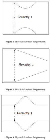
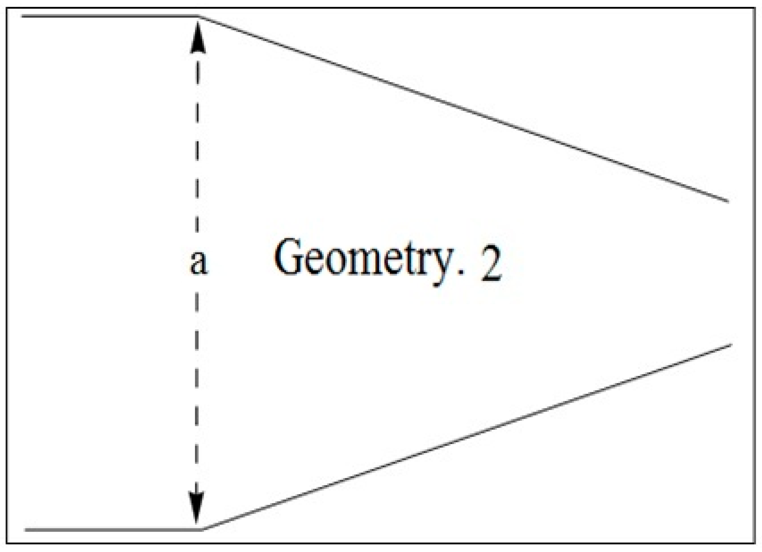
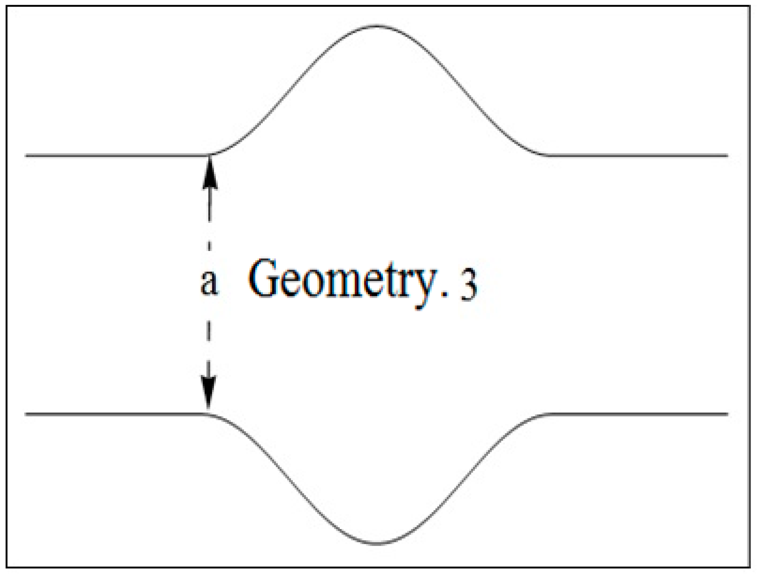
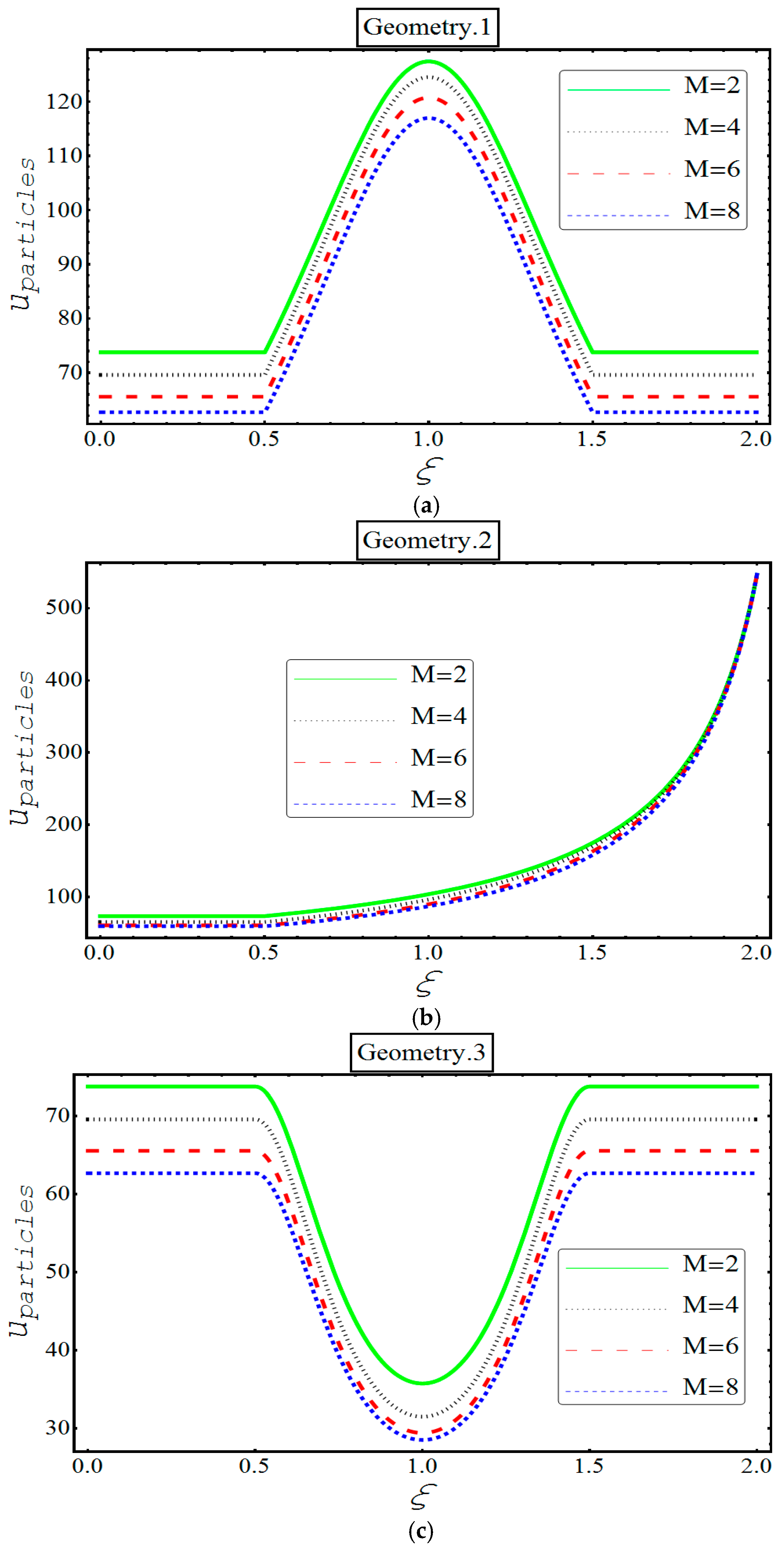
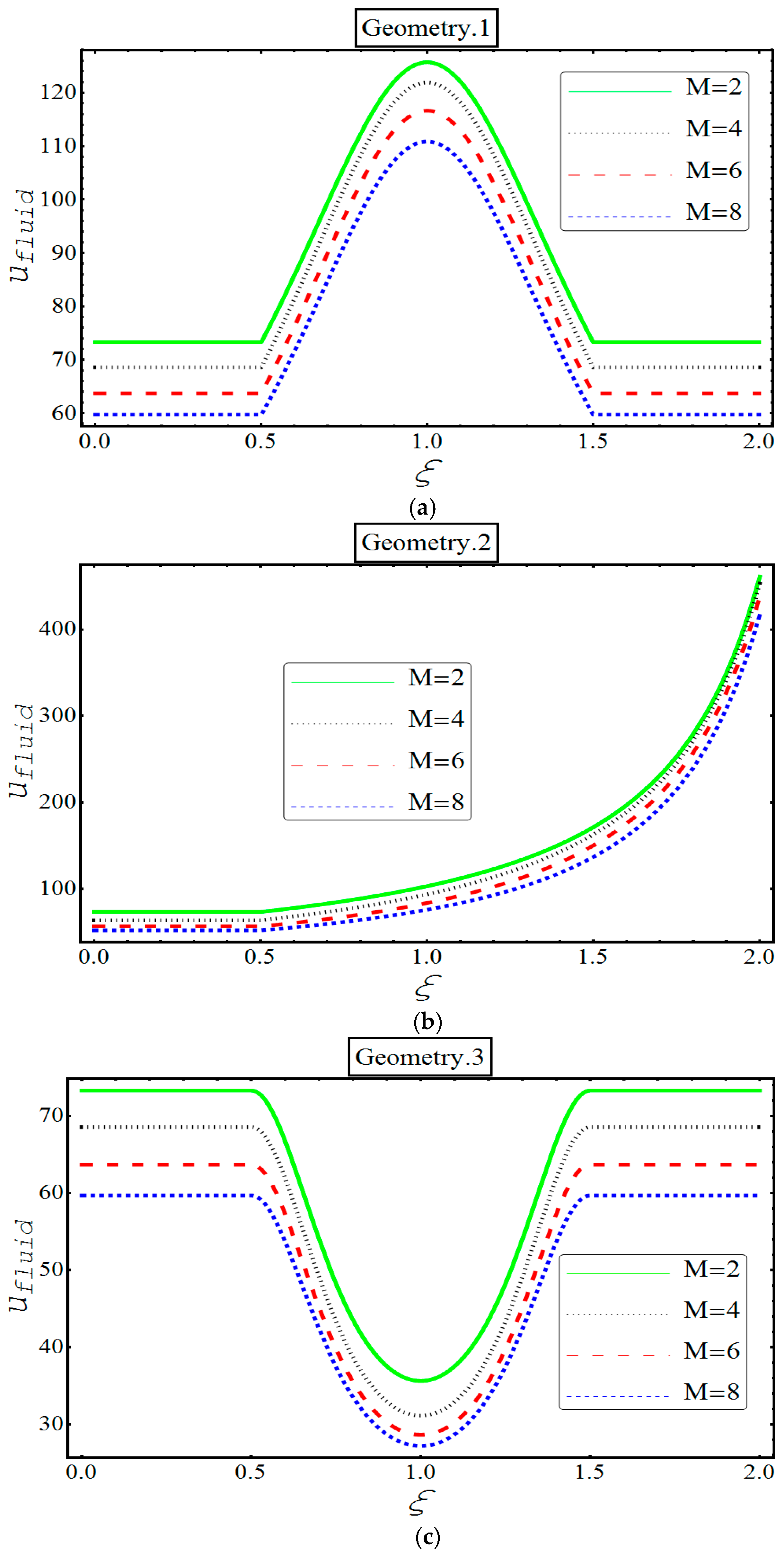
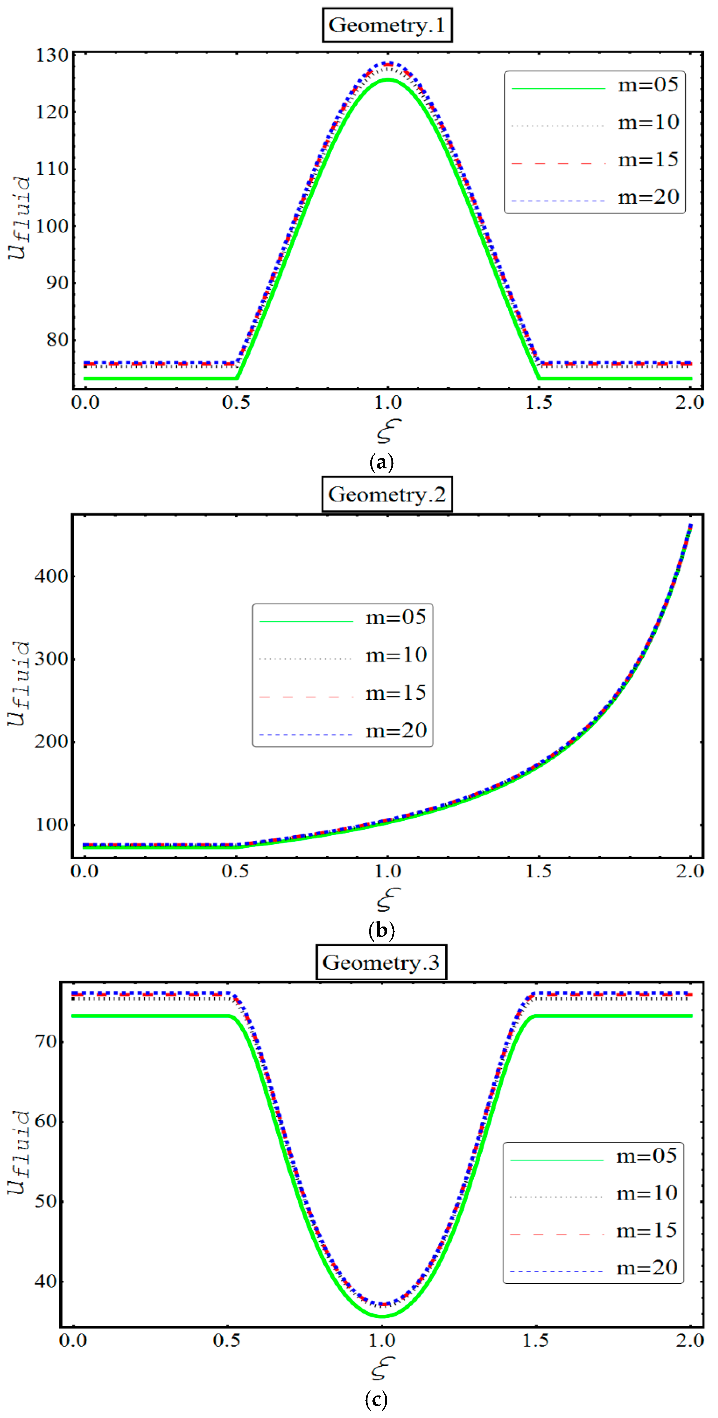
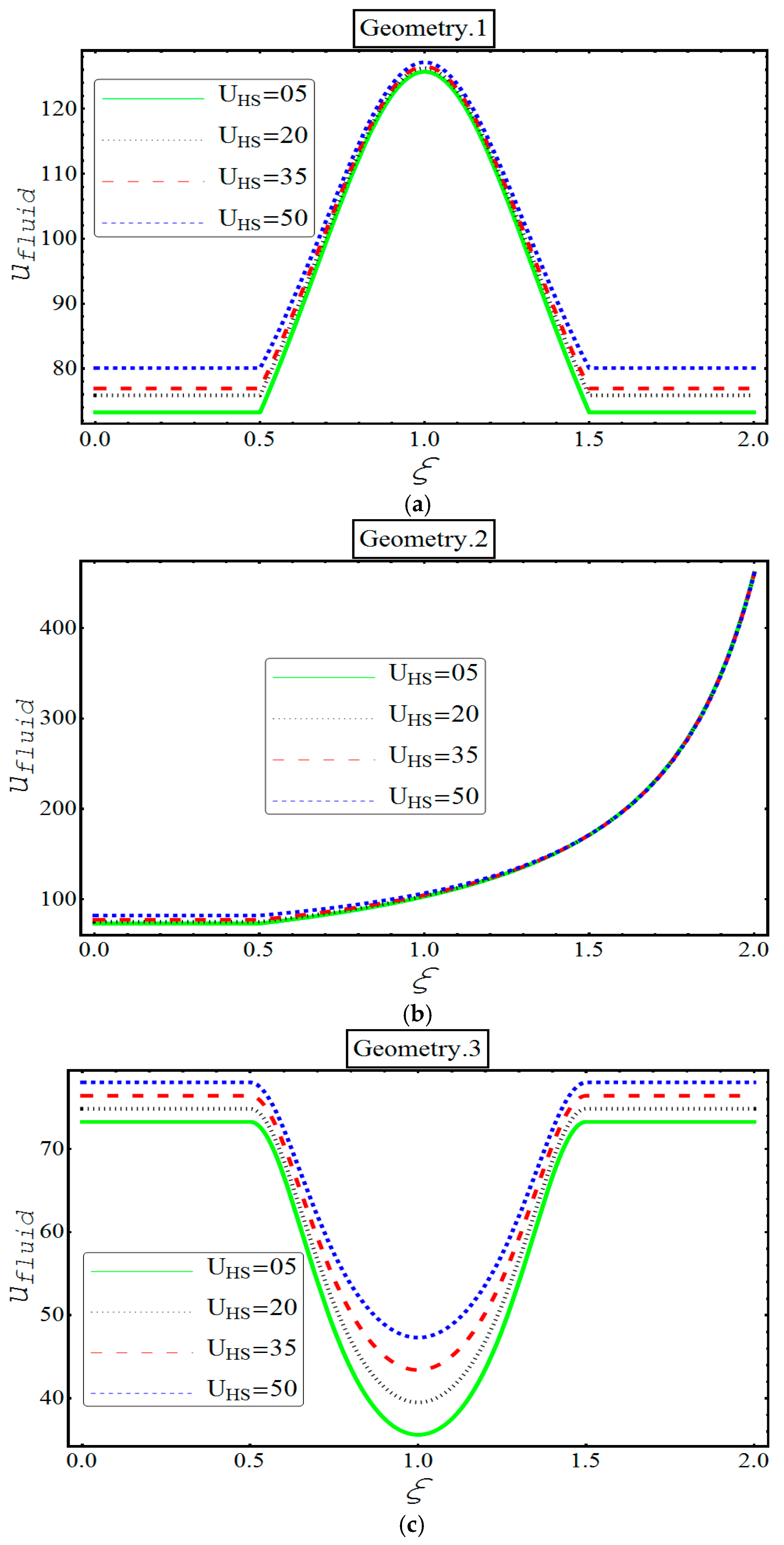
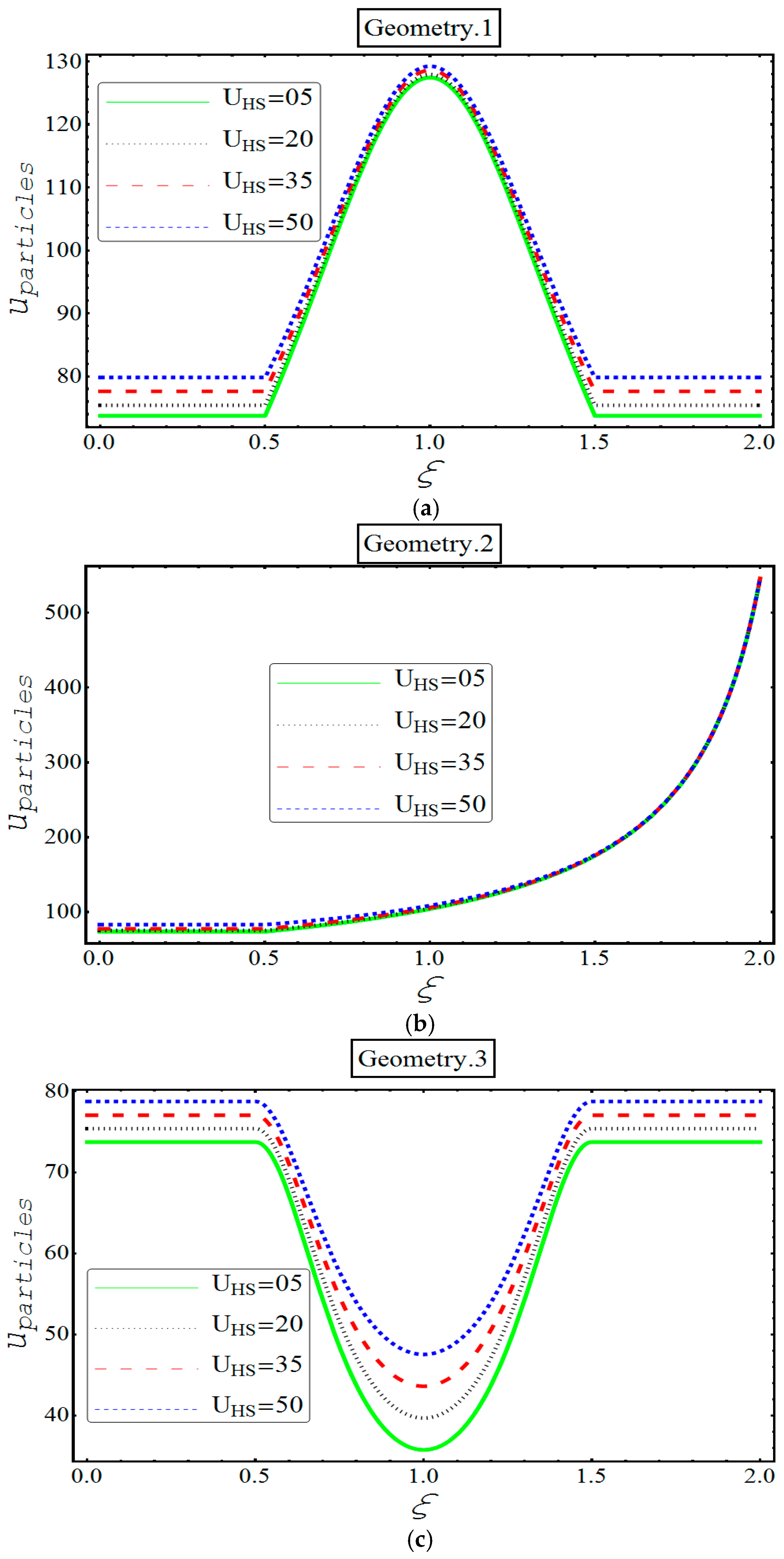
Decrease in the behavior of both fluid and particle velocity, is found in third geometry and it is because of central ‘bulging out’ corrugation.
Velocity of each phase loses its strength for different values of Hartmann number in all geometries.
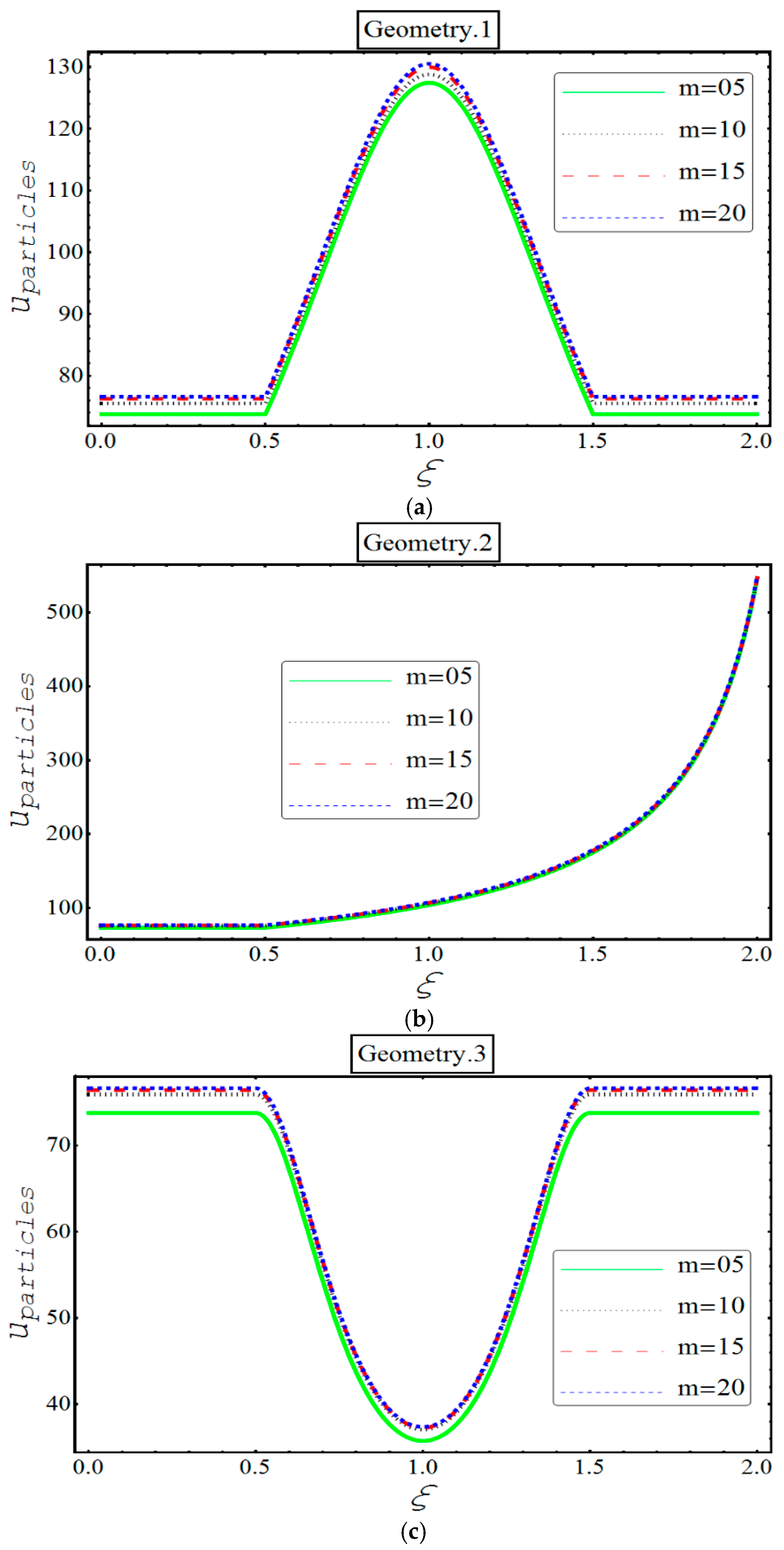
An apparent incline in the velocity of both phases is observed in all three geometries for various values of U H S and m .
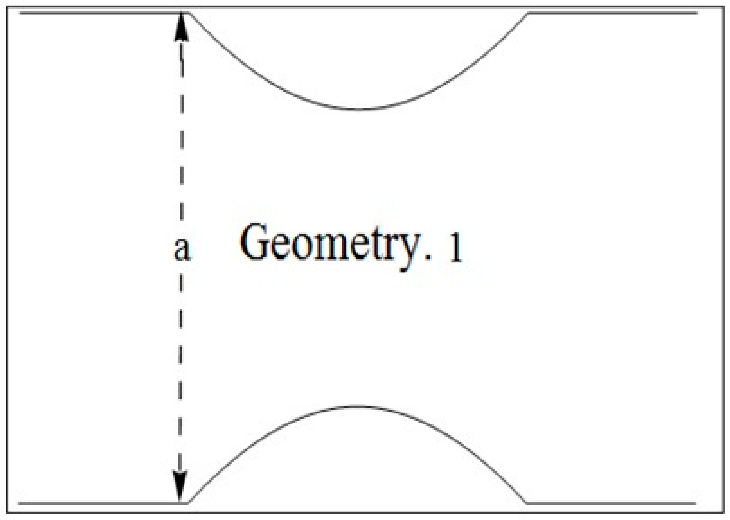
Unlike in other geometries, only in second geometry, the velocity of each phase keeps on increasing indefinitely. This unique feature can be termed because of the bent ‘bellows’ structure of the channel.
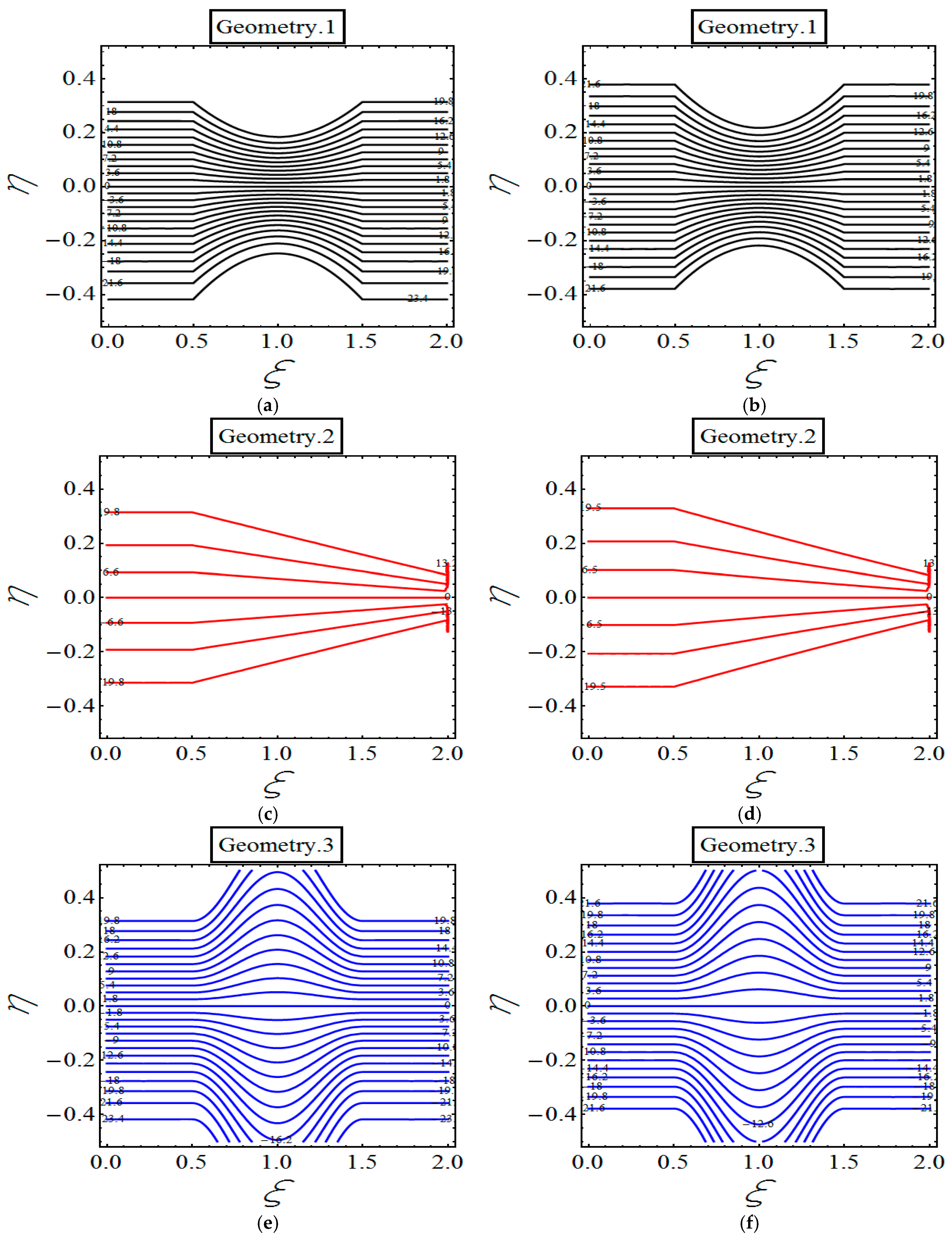
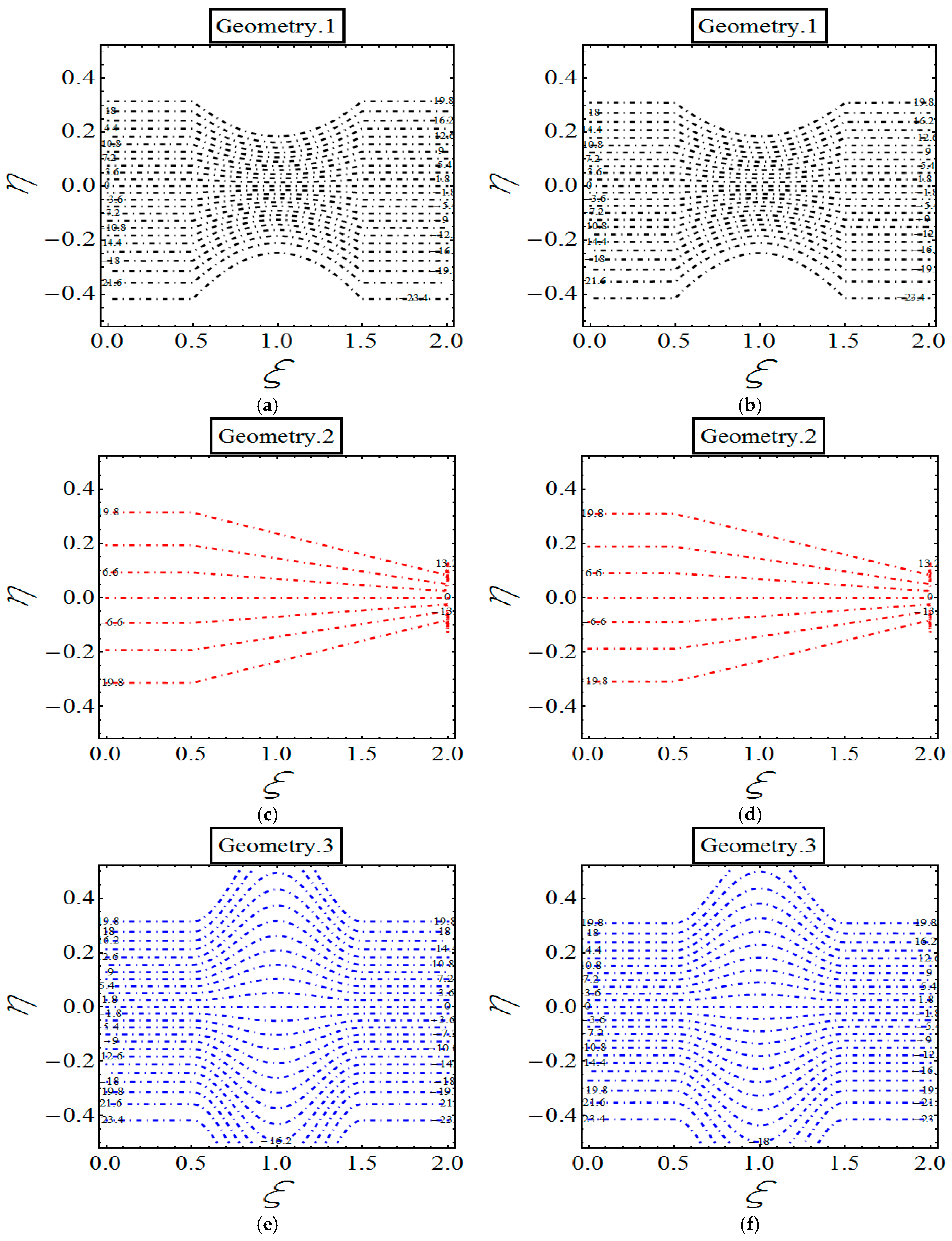
Emergence of extra stream lines in all geometries in response of strengthening the magnetic field.
Reduction in stream lines for m solely observed in first geometry.
In the case of U H S , flow patterns in all geometries remain same.

Acknowledgments

F. Hussain is grateful to the Higher Education Commission (HEC) Pakistan for awarding him indigenous scholarship for his PhD studies.

Author Contributions

This paper is contributed in all respect by all authors equally.

Conflicts of Interest

The authors declare no conflict of interest.

References

  1. Chamkha, A.J. Solutions for fluid-particle flow and heat transfer in a porous channel. Int. J. Eng. Sci. 1996, 34, 1423–1439. [Google Scholar] [CrossRef]
  2. Khan, U.; Adnan, M.; Ahmed, N. Soret and Dufour effects on Jeffery-Hamel flow of second-grade fluid between convergent/divergent channel with stretchable walls. Results Phys. 2017, 7, 361–372. [Google Scholar] [CrossRef]
  3. Malvandi, A.; Ghasemi, A.; Ganji, D. Thermal performance analysis of hydromagnetic Al2O3-water nanofluid flows inside a concentric micro annulus considering nanoparticle migration and asymmetric heating. Int. J. Therm. Sci. 2016, 109, 10–22. [Google Scholar] [CrossRef]
  4. Misra, J.C.; Chandra, S. Electro-osmotic flow of a second-grade fluid in a porous microchannel subject to an AC electric field. J. Hydrodyn. 2013, 25, 309–316. [Google Scholar] [CrossRef]
  5. Nadeem, S.; Akram, S. Influence of inclined magnetic field on peristaltic flow of a Williamson fluid model in an inclined symmetric or asymmetric channel. Math. Comput. Model. 2010, 52, 107–119. [Google Scholar] [CrossRef]
  6. Chamkha, A.J. Hydromagnetic two-phase flow in a channel. Int. J. Eng. Sci. 1995, 33, 437–446. [Google Scholar] [CrossRef]
  7. Hank, S.; Favrie, N.; Massoni, J. Modeling hyperelasticity in non-equilibrium multiphase flows. J. Comput. Phys. 2017, 330, 65–91. [Google Scholar] [CrossRef]
  8. Dong, S. Wall-bounded multiphase flows of immiscible incompressible fluids: Consistency and contact-angle boundary condition. J. Comput. Phys. 2017, 338, 21–67. [Google Scholar] [CrossRef]
  9. Hayat, T.; Sajjad, R.; Ellahi, R.; Alsaedi, A.; Muhammad, T. Homogeneous-heterogeneous reactions in MHD flow of micropolar fluid by a curved stretching surface. J. Mol. Liq. 2017, 240, 209–220. [Google Scholar] [CrossRef]
  10. Awais, M.; Aqsa; Malik, M.Y.; Awan, S.E. Generalized magnetic effects in a Sakiadis flow of polymeric Nano-liquids: Analytic and numerical solutions. J. Mol. Liq. 2017, 241, 570–576. [Google Scholar] [CrossRef]
  11. Sheikholeslami, M.; Bhatti, M.M. Active method for nanofluid heat transfer enhancement by means of EHD. Int. J. Heat Mass Transf. 2017, 109, 115–122. [Google Scholar] [CrossRef]
  12. Hassan, M.; Zeeshan, A.; Majeed, A.; Ellahi, R. Particle shape effects on ferro fluid flow and heat transfer under influence of low oscillating magnetic field. J. Magn. Magn. Mater. 2017, 443, 36–44. [Google Scholar] [CrossRef]
  13. Khan, M.; Hashim; Hussain, M.; Azam, M. Magnetohydrodynamic flow of Carreau fluid over a convectively heated surface in the presence of non-linear radiation. J. Magn. Magn. Mater. 2016, 412, 63–68. [Google Scholar] [CrossRef]
  14. Hayat, T.; Muhammad, T.; Ahmad, B.; Shehzad, S. Impact of magnetic field in three-dimensional flow of Sisko nanofluid with convective condition. J. Magn. Magn. Mater. 2016, 413, 1–8. [Google Scholar] [CrossRef]
  15. Bhatti, M.M.; Abbas, T.; Rashidi, M.M.; Ali, M.E.; Yang, Z. Entropy generation on MHD Eyring-Powell nanofluid through a permeable stretching surface. Entropy 2016, 18, 224. [Google Scholar] [CrossRef]
  16. Daskiran, C.; Liu, I.; Oztekin, A. Computational study of multiphase flows over ventilated translating blades. Int. J. Heat Mass Transf. 2017, 110, 262–275. [Google Scholar] [CrossRef]
  17. Raza, J.; Rohni, A.M.; Omar, Z.; Awais, M. Heat and mass transfer analysis of MHD nanofluid flow in a rotating channel with slip effects. J. Mol. Liq. 2016, 219, 703–708. [Google Scholar] [CrossRef]
  18. Haq, R.U.; Kazmi, S.N.; Mekkaoui, T. Thermal management of water based SWCNTs enclosed in a partially heated trapezoidal cavity via FEM. Int. J. Heat Mass Transf. 2017, 112, 972–982. [Google Scholar] [CrossRef]
  19. Raza, J.; Rohni, A.M.; Omar, Z.; Awais, M. Rheology of the Cu-H2O nanofluid in porous channel with heat transfer: Multiple solutions. Phys. E Low Dimens. Syst. Nanostruct. 2017, 86, 248–252. [Google Scholar] [CrossRef]
  20. Haq, R.U.; Rashid, I.; Khan, Z.H. Effects of aligned magnetic field and CNTs in two different base fluids over a moving slip surface. J. Mol. Liq. 2017, 243, 682–688. [Google Scholar] [CrossRef]
  21. Tripathi, D.; Bhushan, S.; Anwar Beg, O. Transverse magnetic field driven modification in unsteady peristaltic transport with electrical double layer effects. Colloids Surf. A Physicochem. Eng. Asp. 2016, 506, 32–39. [Google Scholar] [CrossRef]
  22. Mohyud-Din, S.T.; Khan, U.; Ahmed, N.; Hassan, S.M. Magnetohydrodynamic flow and heat transfer of nanofluids in stretchable convergent/divergent channels. Appl. Sci. 2015, 5, 1639–1664. [Google Scholar] [CrossRef]
  23. Khan, W.G.; Idrees, T.; Islam, M.; Khan, S.; Dennis, L.C. Thin film Williamson nanofluid flow with varying viscosity and thermal conductivity on a time-dependent stretching sheet. Appl. Sci. 2016, 6, 334. [Google Scholar] [CrossRef]
  24. Sheikholeslami, M.; Ellahi, R. Electrohydrodynamic nanofluid hydrothermal treatment in an enclosure with sinusoidal upper wall. Appl. Sci. 2015, 5, 294–306. [Google Scholar] [CrossRef]
  25. Sheikholeslami, M.; Zia, Q.M.; Ellahi, R. Influence of induced magnetic field on free convection of nanofluid considering Koo-Kleinstreuer-Li (KKL) correlation. Appl. Sci. 2016, 6, 324. [Google Scholar] [CrossRef]
  26. Sekrani, G.; Poncet, S. Further investigation on laminar forced convection of nanofluid flows in a uniformly heated pipe using direct numerical simulations. Appl. Sci. 2016, 6, 332. [Google Scholar] [CrossRef]
  27. Rashidi, S.; Esfahani, J.A.; Ellahi, R. Convective heat transfer and particle motion in an obstructed duct with two side by side obstacles by means of DPM model. Appl. Sci. 2017, 7, 431. [Google Scholar] [CrossRef]
  28. Ellahi, R. Special issue on recent developments of nanofluids. Appl. Sci. 2018, 8, 192. [Google Scholar] [CrossRef]
Figure 1. Physical sketch of the geometry.
Applsci 08 00275 g001
Figure 2. Physical sketch of the geometry.
Applsci 08 00275 g002
Figure 3. Physical sketch of the geometry.
Applsci 08 00275 g003
Figure 4. Variation of velocity u f for various Hartmann numbers.
Applsci 08 00275 g004
Figure 5. Variation of velocity u p for various Hartmann numbers.
Applsci 08 00275 g005
Figure 6. Variation of the velocity u f for various electro-osmotic parameters.
Applsci 08 00275 g006
Figure 7. Variation of the velocity u p for various electro-osmotic parameters.
Applsci 08 00275 g007
Figure 8. Variation of the velocity u f for various Helmholtz–Smoluchowski parameters.
Applsci 08 00275 g008
Figure 9. Variation of the velocity u p for various Helmholtz–Smoluchowski parameters.
Applsci 08 00275 g009
Figure 10. Stream lines for various Hartmann numbers M = 2 (a,c,e) and M = 5 (b,d,f) in three geometries.
Applsci 08 00275 g010
Figure 11. Stream lines for various electro–osmotic parameters m = 2 (a,c,e) and m = 5 (b,d,f) in three geometries.
Applsci 08 00275 g011
Figure 12. Stream lines for various Helmholtz–Smoluchowski velocities U H S = 2 (a,c,e) and U H S = 5 (b,d,f) in three geometries.
Applsci 08 00275 g012

