1. Introduction
For the generation of a digital terrain model (DTM), it is necessary to identify the terrain points on the bare earth surface. Thus, all non-terrain-points such as vegetation, buildings and other constructions above the ground must be removed, which is referred to as filtering in this context [
1].
There are different approaches for filtering laser scanning data. Some examples of basic algorithms, which have been modified in many ways, are mathematical morphology [
2,
3], interpolation-based [
4], and triangulated irregular network (TIN)-densification. By using geometrical values such as distances and angles as filter criteria [
5], algorithms progressively densify the digital terrain model (DTM) to approximate the bare earth [
6,
7].
These common ground modelling methods have been manly developed for airborne laser scanning (ALS) data and are not optimally suited for ground level determination from terrestrial laser scanning (TLS) data.
The intrinsic point cloud densities, scanning distances, the distribution of noise points and the backscattering geometry of TLS data vary significantly when compared to ALS data. As a terrestrial laser scanner is located within the target area, complete occlusion to some viewing directions is highly probable. The spatial distribution of TLS points are heavily concentrated around the immediate vicinity of the scanner, resulting in excessively high point cloud densities near the scanner that become detrimental for the point cloud processing [
8].
Further, many ground filtering techniques are limited in application within challenging topography and experience difficulty coping with some objects such as short vegetation, steep slopes, and so forth. Lastly, due to the large size of point cloud data, operations such as data traversing, multiple iterations, and neighbour searching significantly affect the computation efficiency [
9].
Some methods have been developed especial for TLS data to segment into ground and non-ground points.
Brodu and Lague [
10] present a supervised classification method using multi-scale dimensionality analysis based on the geometric characteristics of the scene. Combining this information from different scales can build signatures of the scene at each point. This signature can then be used to discriminate vegetation from soil for example.
Pirotti et al. [
11] use the information of a multireturn TLS for vegetation mapping. First, the thresholds of the return number and the normalized amplitude of intensity are set to determine possible ground points. Subsequently, a progressive morphological filter is adopted for generating a DTM and digital surface model (DSM) where the maximum and minimum
Z values are used as criteria to apply a dilation and erosion operator.
Lau et al. [
12] separate ground and non-ground of TLS data by using the RGB value.
Liang et al. [
13] developed a scan line continuousness segmentation well suited for trunk detection. The approach is based on the continuity property of the object surface, planar distance and segmentation in horizontal and vertical directions. The one-dimensional segmentations were first performed independently and then combined to groups with similar distances to the scanner.
Che and Olsen [
9] present a fast ground filtering method for TLS data via a Scanline Density Analysis. The process first separates the ground candidates, density features, and unidentified points based on an analysis of point density within each scanline. Then, a region growth using the scan pattern is performed to cluster the ground candidates and further refine the ground points (clusters).
The method of Panholzer and Prokop [
14] and Puttonen et al. [
8] uses a priori information of the TLS configurations and scanner-centred coordinates to determine the ground level. Integrating these coordinates in the filtering process is an important additional filter parameter.
Some of these methods need additional data that are not always available or are made for a special purpose such as tree location mapping. The method presented here is intended to show a way—including new filter information—of distinguishing soil from non-soil points only with basic data (point cloud and coordinates of laser scanner).
2. Materials and Methods
2.1. Preconditions for Filtering Terrestrial Laser Scanning Data
The great difficulty of filtering earth surface point cloud data is that each point is related to some extent to any other point. In the case of Kriging [
15], an attempt is made to take this fact into consideration as far as possible. As soon as a point is removed, it changes the estimated surface model for the points in the closer neighbourhood. The model has to be recalculated under the new, changed conditions. Particularly in the case of non-unambiguous recording areas, a step-by-step elimination of points results in a surface which is plausible for the human observer with certain probability. The process of point cloud filtering must therefore almost necessarily be an iterative process.
The human being can derive when manually filtering point cloud data a certain probability with regard to the correct surface from height values, the distribution, the structure, etc. It is, e.g., very unlikely that there is an abrupt change in the surface. However, in the case of TLS, more than in the case of ALS, it must be taken into account that objects are usually recorded only from one side, resulting in sharp edges as well as larger areas without recorded points (shadows) behind these objects.
The more a point deviates from the surrounding points (e.g., in height), the more likely it is not a ground point. It is difficult to classify these points with a few and unequally distributed neighbouring points. In these areas, the filter process can be at best a rough estimate.
In this extended approach of the HOVE-Wedge-filtering, an attempt was made to simulate the human perceived probability estimates in the form of algorithms by the help of a computer model which is as universally applicable as possible.
2.2. Wedge Iterative (Modified Model)
The work presented is based upon “Wedge-filtering of geomorphologic terrestrial laser scan data” [
14], where the general procedure of the Wedge Absolute method is described. In the following, we explain our modifications that led to the Iterative Method while the basic principle of Wedge Absolute is briefly reproduced for understanding.
In a static terrestrial laser scan, all measured points must be visible from the laser source of the scanner.
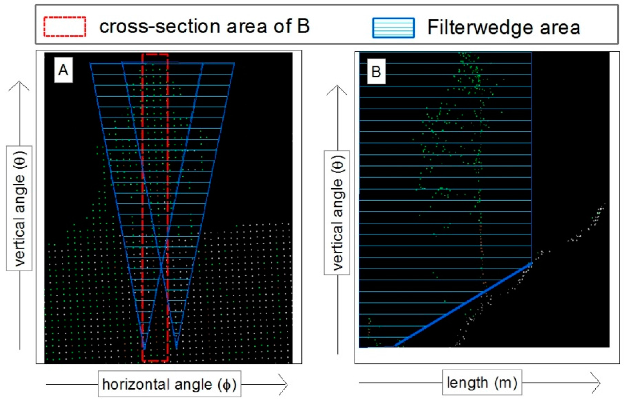
Figure 1A shows a point cloud of terrain from the view of the laser scanner. Connecting each point with the laser source creates a line between the two (blue line in
Figure 1B), given that there were no obstacles along these lines. In the case two connecting lines have the same horizontal angle, the connecting line with the larger vertical angle and smaller measuring distance compared to the connecting line with the smaller vertical angle and greater measuring distance cannot lead to a ground point. Consequently, a point cannot be a ground point if there is a more distant point with a smaller vertical angle in the same direction.
Of course, it is rare that two connection lines have exactly the same direction. Thus, you need to define a threshold. The basic idea is that, for each point, two adjacent points are searched, which are further from the recording point than the point to be checked. The angle is calculated between the connecting line from the recording centre to the recording point and the connecting lines to the adjacent points. The angles are calculated using Equation (1):
where
αli,re is the left or right wedge angle;
∆vert is the difference of the vertical angle; and
∆horz is the difference of the horizontal angle.
For the Wedge Absolute method, if the angular values are greater than a previously defined threshold value, the corresponding recording point is recognized as a non-ground point and will be erased (Equation (2)).
where
αli,re is the left or right wedge angle; and
λTLV is the threshold limit value.
Because the section for the two angle thresholds looks like a wedge (
Figure 1A, blue dashed), we called it the wedge-method. As mentioned in our previous work [
14], this filtering method is not a stand-alone solution for calculating a digital terrain model because it has some weaknesses. The Wedge Absolute method on its own provides satisfactory filtering results only for terrain, without steep inclines.
In contrast to the absolute method in the iterative method, the angle difference to the two adjacent points is calculated for all points. This angle difference is compared with a predefined threshold value. Therefore, an angle difference of 180° means that the point lies precisely in a plane with the two adjacent points. A value greater than 180° indicates that the point is not likely to be deleted. A very small value (acute angle) again indicates a vegetation point. The method to find the two adjacent points is explained in
Section 2.3.3. If the angle difference is less than a certain threshold, the point will be erased (Equation (3)):
where
θdiff is the difference of left (from right adjacent point) and right (from left adjacent point) wedge angle; and
λTLV is the threshold limit value.
2.3. Theory of Filtering over Vertical Horizontal (HOVE) Angular Grid
The method of HOVE grid offers a wide range of possibilities for effective point filtering. Normally, in the case of surface computation, the points are plotted in an X, Y coordinate field. Interpolation then takes place with the inclusion of the Z-coordinate (height). Since the point cloud of terrestrial laser scanners results in a very irregular X, Y coordinate distribution, large areas have to be interpolated or estimated during the generation of height-grid.
A terrestrial laser scanner measures the terrain with a constant angle step in a strip-like manner. If instead of the
X coordinate, we use the horizontal angle (
φ) values and instead of the
Y coordinate, use the vertical angle (
θ) values, an almost perfect, gap-free raster is normally obtained (
Figure 1A). This approach is very similar to the method described by Liang et al. [
13]. An interpolation involving the recording length has several advantages:
The output grid contains no gaps.
It is easier to find terrain structures (e.g., terrain edges).
Quick recalculation of adjacent points is easily computable.
3D filtering is possible.
All information on the search area of the adjacent points can be made in the form of grid spacing, which is normally constant. The grid spacing corresponds to the angle step (θ and φ) of the laser scanner.
The HOVE grid has been used in the following ways.
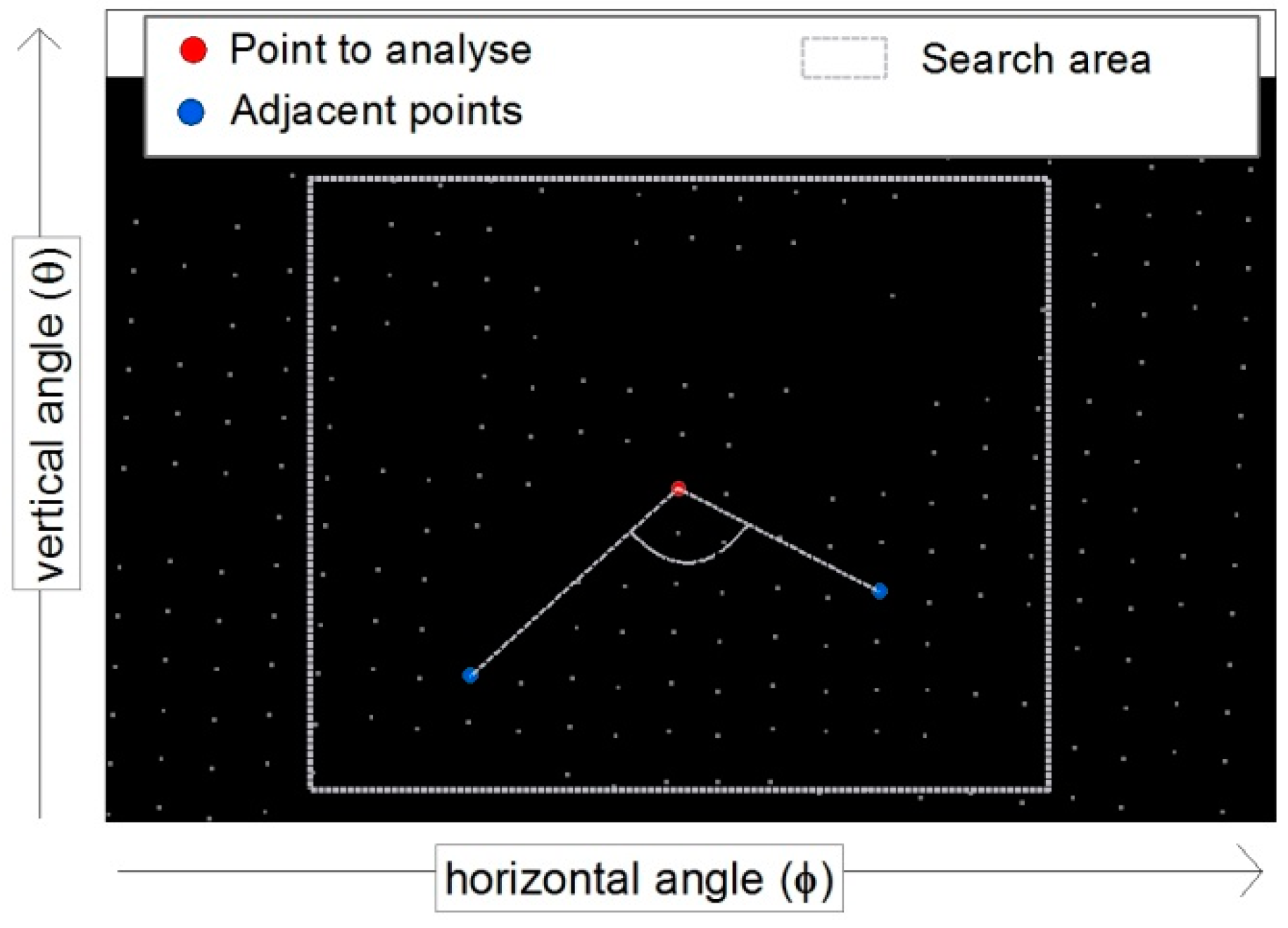
2.3.1. Horizontal and Vertical Angles within the HOVE Grid
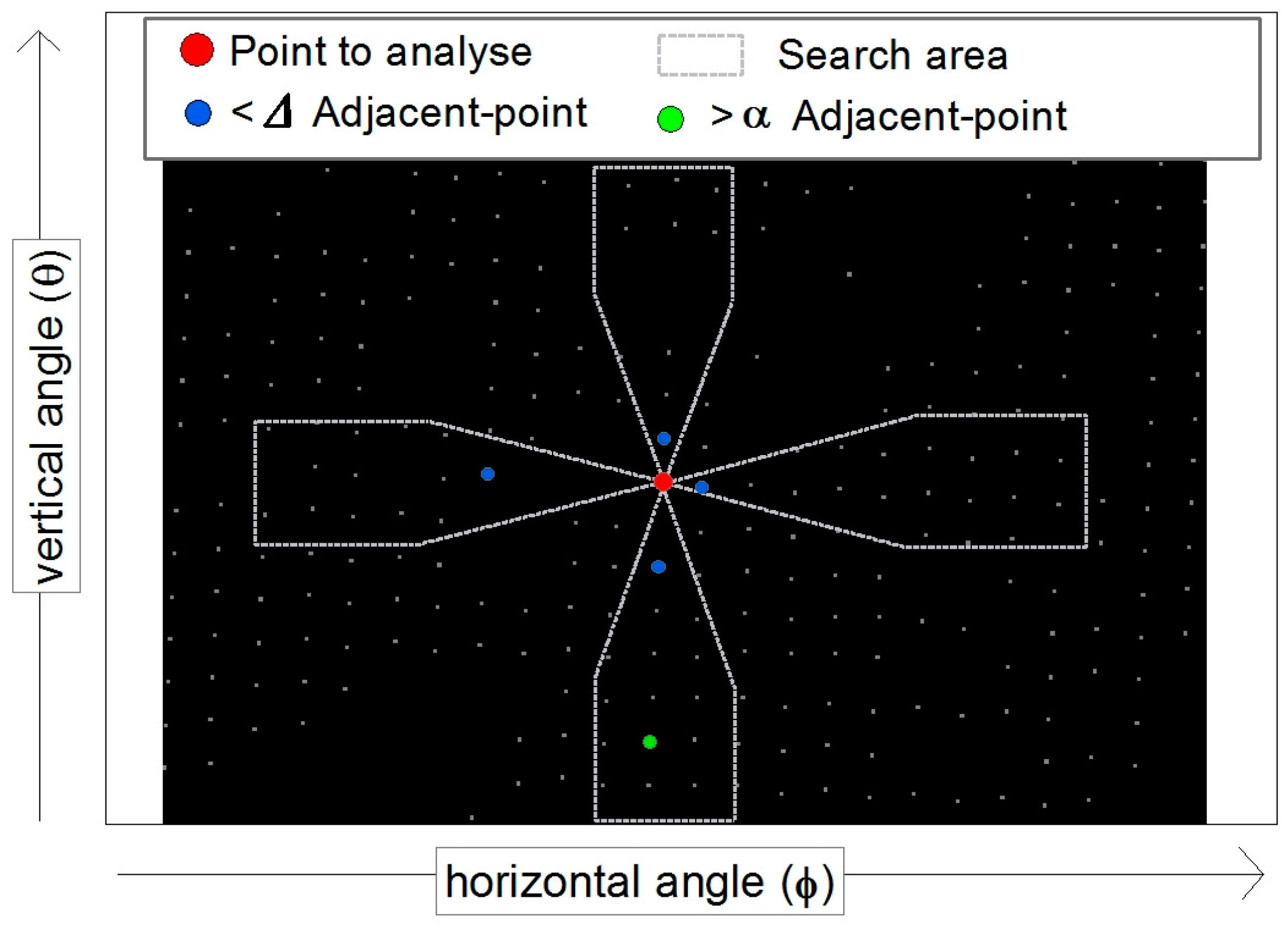
Figure 1A shows a horizontal–vertical angles (HOVE) gird, while
Figure 2 represents a small sector of such a grid. Within the point grid, the closest points above and below as well as to the left and right of the point to be examined are determined (
Figure 2, blue points). For this purpose, the corresponding search area must be defined. Within these search areas, the point with the smallest angular distance to the point to be examined is searched. Subsequently the angle from the examined point to the adjacent points is calculated using Equation (4):
where
αwi is the angle from examined point to adjacent point;
Lpuex is the length from laser scanner to examined point;
Lpuad is the length from laser scanner to adjacent point; and
βpuex is the angle from laser scanner to examined point;
βpuad: angle from laser scanner to adjacent point.
In addition to the closest points, the points with the lowest
αwi below the point to be examined are determined (
Figure 1, green points).
From the angles found, the respective angle difference can be calculated. If no angle could be calculated for one side due to lack of points, the average of the negative angles of the next and after next point on the opposite side was taken for this side. If no closed point angle could be determined fir both sides, the difference of points with the lowest αwi will be used for calculation.
With the help of these angle differences, the following statements on the terrain model can be made.
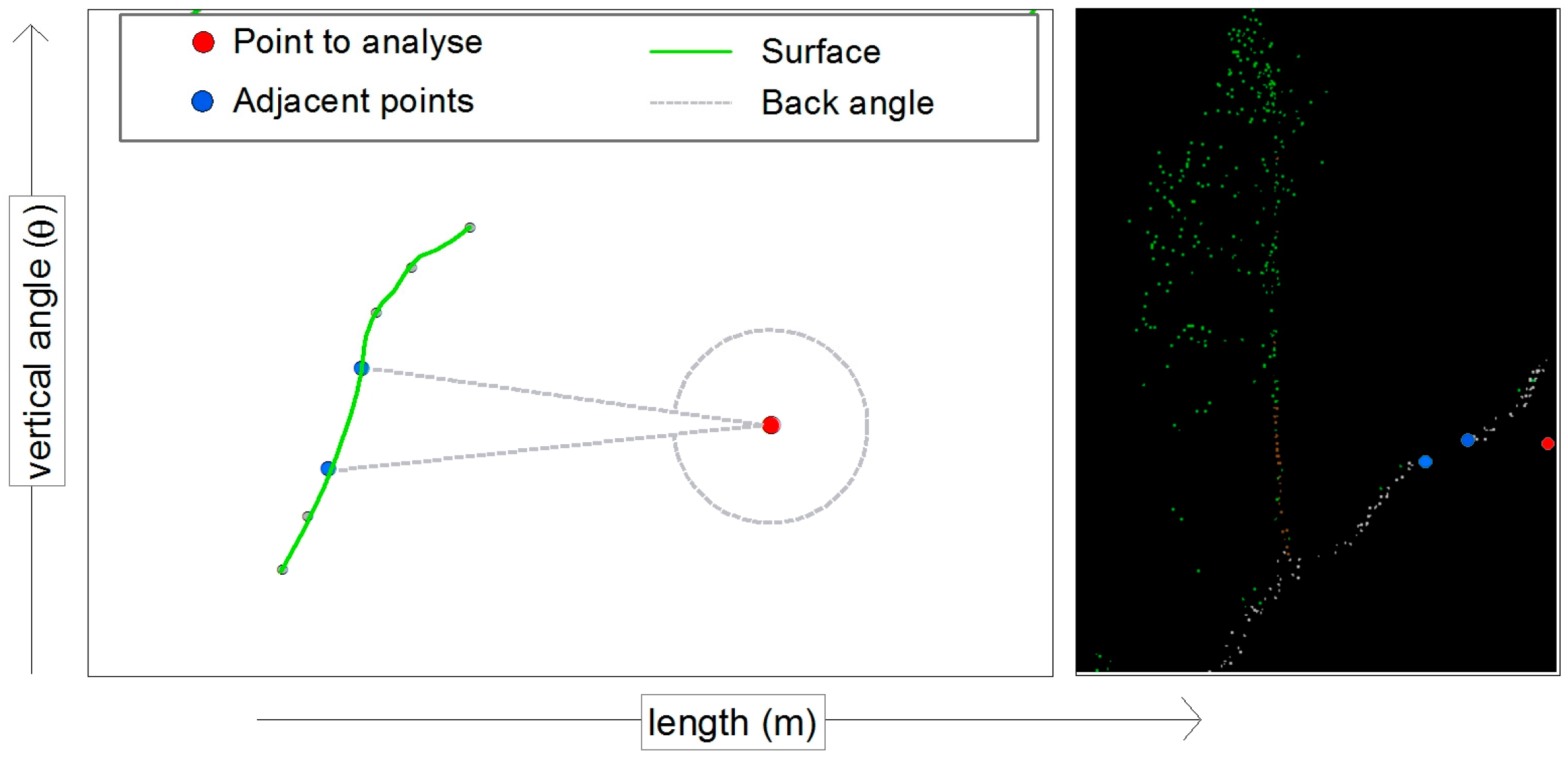
Find Distance Measurement Errors
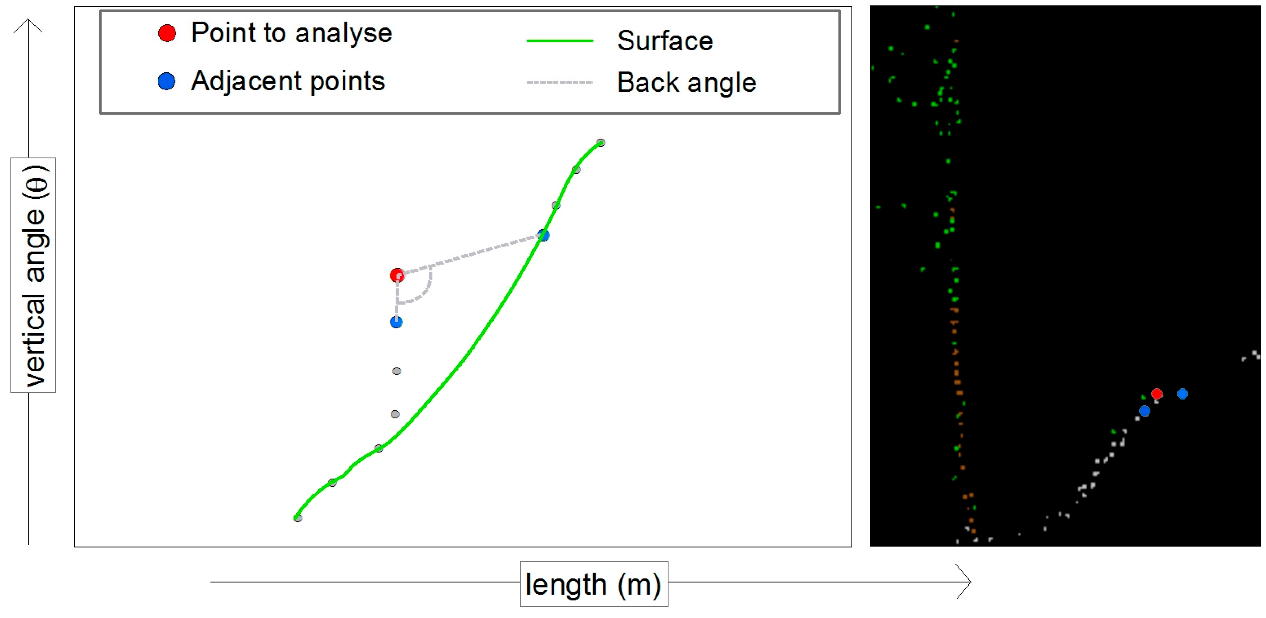
The dataset used includes some points that are obviously measurement errors. Even points which have a remarkably large length must be removed before the ending filtering. These points would otherwise be responsible for removing a lot of correct ground points. To identify these points, in a specific search range for each point, the horizontal as well as vertical back angle-difference to its neighbouring points is calculated. The left side of
Figure 3 shows a schematic representation of the terrain cross-section, where the grey lines correspond with the vertical angles—to the adjacent points above and below the point to analyse—in
Figure 2. The right side should give you an idea how these points could be situated in a cross-section of a measured point cloud.
If this angle difference is greater than a previously defined threshold value, this point is prematurely removed as a measurement error point from the further calculation (Equation (5)):
where
θdive is the difference of the vertical back-angles;
θdiho is the difference of the horizontal back-angles; and
λTLV is the threshold limit value.
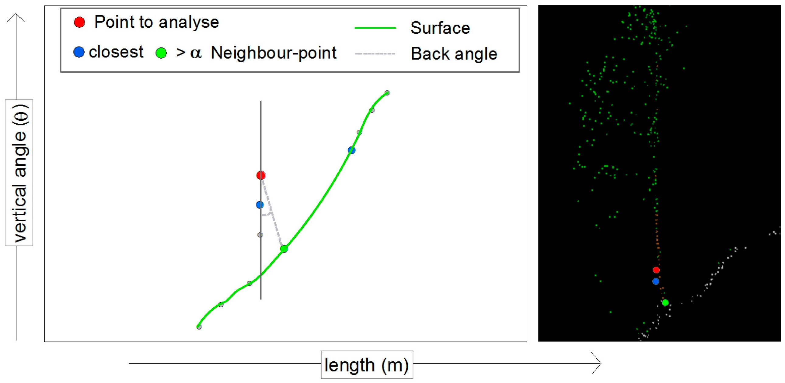
Reduction to a 2.5-Dimensional Terrain
In this step, all points above a connecting line from other points below are removed from a three-dimensional point cloud (
Figure 4). From the remaining points, a 2.5-dimensional terrain can be expected. These points would also be eliminated by Wedge Filtering. Since the filtering is only done iteratively via the wedge angle, the reduction with HOVE grid is more effective.
As described in
Section 2.3.1, beneath the angles to the adjacent points the angle to the point with the lowest α is also calculated. If you take a small cross-section such as the red area in
Figure 1A, points with a higher
θ and shorter length (
Figure 1B) are with high probability vegetation points. The lowest
αwi of such points is less zero. If the angle to the point below with the lowest
αwi is less zero, the examined point will be eliminated:
where
αwi vert below is the angle from examined point to adjacent point below; and
λTLV is the threshold limit value.
Eliminate Vegetation Points
The expected angular difference in flat terrain or a constant steepness is 180°; the smaller this difference angle, the more the relevant point protrudes from its adjacent points. With the decrease in the angle difference, the likelihood of a vegetation point increases correspondingly (
Figure 5).
2.3.2. Determination of the Point Density
The output data form a homogenously distributed grid. Due to the repeated filtering, larger holes are normally occurring in some areas and the initial structure is retained in other areas. Where, after repeated filtering, the initial structure is retained, this indicates a continuous terrain surface without much vegetation. These points should be maintained in the further filtering process. Areas which have large gaps in the grid after some filter repeats, however, indicate that the area is generally flatter and has vegetation. A precise distinction between ground and non-ground point is virtually impossible without precise knowledge of the terrain. An automated algorithm can only calculate with probabilities. The probability of a ground point in areas with low grid point density after few iterative filtering is significantly lower than in areas were high grid point density retained. It therefore makes sense to gradually reduce the threshold value of the Wedge Filtering in these areas depending on the grid point density. A HOVE raster is ideal for determining the point density.
Particularly important is this additional information for small objects, such as hills or edges protruding from the surrounding surface. Such terrain elements are a problem with all filter methods. A remaining high point density after iterative filtering within a certain angular segment and therefore many similar neighbouring points indicates a natural surface even with sharp edges.
Rodriguez-Caballero et al. [
16] propose a method to filter terrestrial laser scanner point clouds using morphological filters and spectral information to conserve surface micro-topography.
2.3.3. Finding the Adjacent Points for Iterative Wedge Filtering
The key point and the great difficulty of wedge filtering are finding the most meaningful neighbours for each point. Within a particular search area of the HOVE grid, all points are determinate which are behind the point to be examined. Therefore, all points with a smaller distance to the recording centre are excluded. Among the remaining points, the right and left sides are searched for the point (
Figure 6) which has the lowest value according to the Equation (7):
minli,re is the minimum value;
∆vert is the difference of the vertical angle (from laser scanner);
∆horz is the difference of the horizontal angle (from laser scanner);
fakt is the factor for
∆horz;
diwi is the average HOVE raster resolution; and
∆len is the difference of length (from laser scanner).
If in the HOVE grid the adjacent point is above the point to be examined (positive vertical difference), the formula value increases. If the neighbouring point lies below the point to be examined (negative vertical difference), the formula value decreases. By the factor, the influence ratio of the horizontal and vertical difference can be weighted. The distance to the point behind is also taken into account by the length difference, whereby the multiplication with the average raster resolution ensures the size adaption to the angle differences.
3. Results
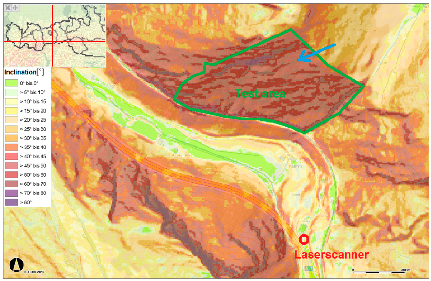
3.1. Description of the Test Area
The test area is located in the hamlet Lueg near the village of Gries am Brenner in Tyrol, Austria. We took measurements of the south-facing slopes of the Padauner Kogel. Below this mountain slope runs the railway track of the Brennerbahn, which is today a part of one of the most important railway connections between Germany and Italy. It connects Munich via Innsbruck with Verona on the shortest route. This section of the track is strongly endangered by rockfall and is protected by numerous protective structures. Due to their rapid evolution, high velocity and impact energy and proximity to infrastructure, mass movements can pose a significant natural hazard. Such mass movements of different types have been surveyed extensively by terrestrial laser scanning in the past [
17,
18,
19]. According to Abellan et al. [
20], the key insights into the use of terrestrial laser scanning (TLS) in rock slope investigations include: (a) the capability of remotely obtaining the orientation of slope discontinuities, which constitutes a great step forward in rock mechanics; and (b) the possibility to monitor rock slopes which allows not only the accurate quantification of rockfall rates across wide areas but also the spatio-temporal modelling of rock slope deformation with an unprecedented level of detail. The purpose of this laser scanning is to be able to carry out an improved risk analysis for this area by means of a very detailed surface model.
In addition to the automated filtering, we manually categorized points into ground and non-ground points. The manually filtered results are therefore suitable for comparison with results from automated filtering methods.
The surveyed slope is approximately 1 km long and has a height difference between valley and mountain tops of approximately 450 m. Most of the area has vegetation, manly the steep parts are rock without vegetation with slope up to 70°. Because of the diverse terrain, automated filtering of laser scanning data is difficult.
Figure 7 shows an inclination map [
21] of the test site. Flat areas have brighter colours as mostly barren slopes with more than 60° inclination. Two significant, large rock formations are on the upper side and at the left below.
3.2. DEM Calculation of the Test Areas Using the Modified Wedge Filtering Method
For the calculation of the new filter method, the VB.NET program mentioned in the article “Wedge-Filtering of Geomorphologic Terrestrial Laser Scan Data” [
14] was further developed.
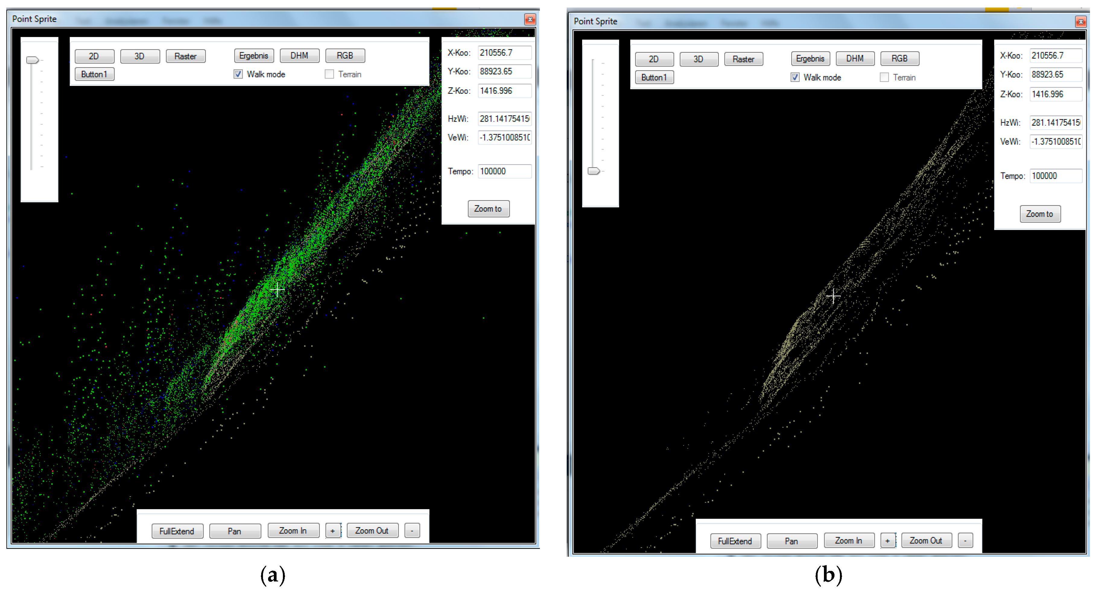
Figure 8a shows a screenshot of the VB.Net program, in which a small section of the test area view is seen from the side (blue arrow in
Figure 7). The vegetation points are still in green colour. In
Figure 8b, these vegetation points are no longer shown for the same section. The points, which are shown in brown colour, remain, which were classified as soil points in the filter process and give a homogeneous surface structure.
Steps of Calculation
Calculate the horizontal and vertical angles as well as the length distances from the recording centre to every single point.
Determine the average raster spacing of the horizontal–vertical angle grid.
Eliminate measuring errors, as described in
Section 2.3.1, Point (a). An angle of 179° was chosen as the threshold value.
Reduce to 2.5D, as described in
Section 2.3.1, Point (b). With this step, approximately 40% of the points are eliminated from the further calculation.
Perform HOVE-Wedge Filtering as described in
Section 2.3. This process is carried out iteratively, until no further point is eliminated. The wedge angles (see
Section 2.3.3), horizontal and vertical angles of the HOVE-grid (see
Section 2.3.1) and point density (points within a certain angular segment, see
Section 2.3.2) have influence in Equation (8):
where
θwedge is the difference of wedge angle;
θvert is the difference of vertical angle from HOVE-Raster;
θhori is the difference of horizontal angle from HOVE-Raster;
F is the weight factors;
λTLV is the threshold limit value; and
density is the value of point-density from HOVE-Raster.
As threshold limit value, we used 200. With the factors, it would be possible to weight the difference. In the calculation, all factors were set to one.
3.3. Calculation and Accuracy of Digital Elevation Model (DEM)
To obtain a digital elevation model (DEM), we interpolate the calculated ground points using ArcGIS by ESRI Inc. (380 New York Street, Redlands, CA 92373, USA). According to ESRI [
22], the Natural Neighbour method is also well suited for distributed point clusters, for example from terrestrial laser scan recordings.
The equation for the Natural Neighbour (NN) interpolation is:
where
G(
x,
y) is the NN estimation at (
x,
y);
n is the number of nearest neighbours used for interpolation;
f(xi,yi) is the observed value at (
xi,
yi); and
wi is the weight associated with
f(
xi,
yi).
Based on the computed results, we calculated a digital elevation model (DEM) with a cell size of one meter. For the evaluation of the results, we used a DEM of the test areas, where the non-ground points had been filtered out manually by optical valuation before. We calculated the difference between the automated filtered DEM and the manually filtered DEM.
In addition to the results of the new filter approach we described, we compared DEMs of the test areas with the results of the automated filter methods described by Prokop and Panholzer [
14].
To evaluate the accuracy to the reference DEMs, we calculated the mean error and the root-mean-square-error (RMSE). According to the ASPRS (American Society for Photogrammetry and Remote Sensing) Guidelines [
23] and Gianinetto and Fassi [
24], the RMSE is often used to assess the accuracy of elevation data and is defined as (10):
where
∆Zi are the elevation residuals (i.e., the differences of the elevation measures with respect to reference data);
n is the number of measures.
Höhle et al. [
25,
26] further recommend using the median, the normalized median absolute (NMAD), the standard deviation, the 68.3% quantile and the 95% quantile of absolute residuals for accuracy assessment of DEMs.
3.4. Results of the Test Area
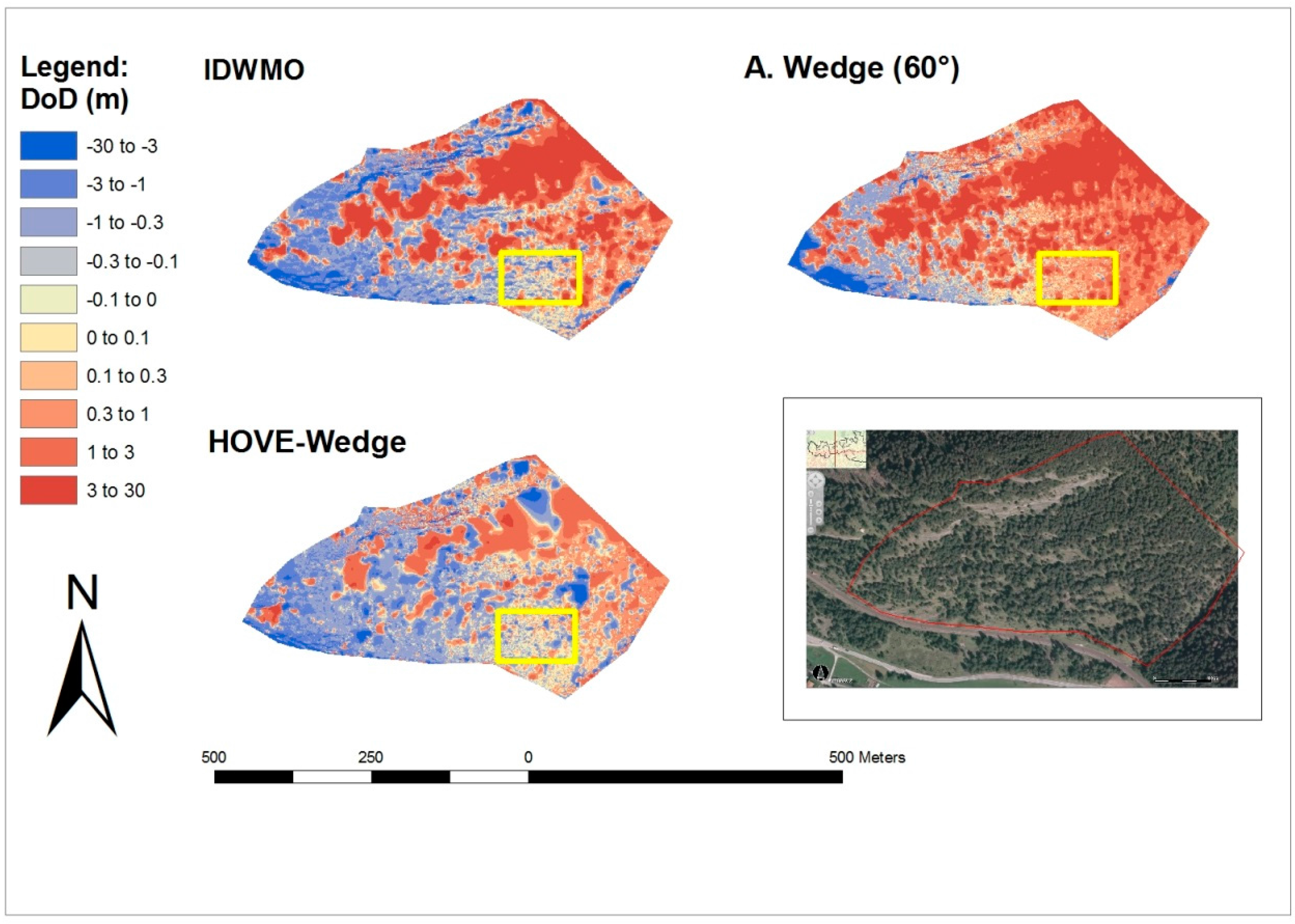
Figure 9 shows the individual differences between the newly calculated DEMs and the manually filtered DEM (DoD = Differences of DEMs). The areas with warm colour indicate a good match between the DEMs. The red areas indicate where the newly calculated DEMs are above the reference model, resulting from an insufficient filter effect. Blue areas indicate where the newly calculated DEM is lower than the reference model due to faulty filtered ground points.
After the manual filtering of the point data, only a few points remained in the centre of the test area. Due to the lack of ground points, the significance of the filter effect in this area is low. Consequently, the statistical values are distorted for the entire recording area. Therefore, we have selected a specific area with a high point density for further analysis. In this area, the statistical inaccuracies are largely avoided and thus more significant results are achieved.
As a result of the HOVE-wedge-filtering, we identified 23,135 ground points and 55,634 non-ground points. The mean error of the two surfaces is −0.07 m with a RMSE of 1.610 and a standard deviation of 1.609 (
Table 1).
Especially in the forested areas near the laser scanner, an area with high point density, we see a better filter effect, as indicated by the larger warm coloured zones in
Figure 9. In the more distant forested areas, the filtering effect is reduced, recognizable by the large red areas in the centre of
Figure 9. In this area, only the highest tops of the trees could be recorded, since it is unlikely that the laser beam penetrates to the ground of such forested areas. Therefore, effective filtering is difficult.
Looking at the figure, we can see that in the part of the HOVE-wedge there are fewer dark red areas than in the other two filtering methods. This indicates that vegetation has been filtered out well.
In
Figure 10, some areas with great optical significance for quality of the filtering were worked out. Detail 1 shows a protruding formation sloping to three sides. In such terrain forms, the filtering is extremely difficult, since high angular differences caused by the terrain edges have influence to the calculation formula. If the threshold value is set too low, this rock ledge is incorrectly removed during filtering. The blue points in Detail 1 show the result at a threshold of 160, the yellow points show the points which are not eliminated with a threshold of 200, the red which are not eliminated at a threshold of 240. For Detail 2, the results from the calculation with a threshold of 160 (blue points) are compared with the results from the calculation with a threshold value of 240 (red points). These points are very difficult to detect as ground points by an automated analysis, since the terrain in this area drops sharply (high angle difference) and only a few neighbouring points are present (small density factor). The optical evaluation classification as probable ground points is only possible with the inclusion of remote environmental parameters. It is difficult to automate an inclusion of such remote environmental parameters because the inclusion of wrong (e.g., not yet properly filtered) point regions would affect the filter result negatively. Hence, the dilemma is, for an optimal filtering of the individual points one needs already filtered and thus meaningful environmental parameters, which at that time but not yet exist. A step-by-step approach to the best result seems therefore necessary. Detail 3 marks a relatively flat, densely wooded section. A very small threshold value would be advantageous as mentioned above. Due to the extremely small number of points, it is not possible to opt for any terrain shapes. A distinction in ground points and non-ground points in this area is often only speculation. An automated analysis with low error probability is thus not possible here.
Detail of Test Area with a High Point Density
The objective of the following assessment is to understand how the wedge filter works under more homogeneous conditions. Therefore, we calculated statistical values for a sample of the first test area (
Figure 9, yellow rectangles). The resulting statistical values are summarized in
Table 2.
When looking at the statistical evaluation, it can be seen that the extent of the qualitative improvement of the results with the HOVE-Wedge method in the area with a high point density is even a little bit higher than in the results of the overall recording. Thus, the standard deviation from 1.537 (Wedge Absolute) or 1.366 (IDWMO) could be reduced to 0.536, which corresponds to an improvement of 186 (Wedge Absolute) or 155 (IDWMO) percent. The percentage improvement of the standard deviation over the entire test area is only 174 percent versus the absolute wedge method and 97 percent versus the IDWMO method.
4. Discussion
The fact that the improvement of the detail area is better than over the entire test area is explained by the fact that the iterative calculation in combination with sufficient environmental information by close neighbouring points can lead to good prediction about the probability of the point status. In areas with few or no neighbouring points and thus poor environmental information, no good predictions can be made. Therefore, many non-ground points are not recognized as such.
The inclusion of the HOVE grid allows additional, valuable conclusions about the real terrain. As mentioned, this approach is very similar to the method described by Liang et al. [
13] where the point cloud data were also plotted with the horizontal angle (
θ) values and the vertical angle (
φ) values. In difference to the HOVE method, where filtering is done with the angles to the adjacent points, the filtering of the tree trunks bases on the principles of scan line segmentation [
27]. The method of scan line segmentation is suitable to find planar objects, but it is difficult to segment uneven surfaces with few points left.
The HOVE method alone can also be used for three-dimensional filtering. While, in the HOVE grid, the angular deviation is calculated from the measuring lengths, the angle calculation in the Wedge method is done using the height value or the Z-coordinates. Since the lengths of the TLS are usually measured from the side, the combination of these two methods provides information from two sides. This leads to more meaningful results. A more accurate analysis of adjacent grid point data to each other in the form of interpolation would be a next step toward increasing accuracy. However, interpolation is not easy in this case. Because of the irregular distribution of the points, a non-directional method (e.g., IDW) is not useful. The spline method would probably be a suitable interpolation method.
Because terrestrial laser scans are usually taken from the side, a HOVE-grid window can contain points of two different terrain formations (e.g., small hill before large mountain). The points of the frontal formation may not be included in the interpolation of the formation behind. A preliminary separation of the points of the respective formation via the recording lengths or automated edge detection is therefore necessary before an interpolation can be made.
A further improvement could be achieved by the combination of point clouds measured from different recording directions. A small change of the recording centre could already lead to a large information gain.
In any case, there is still potential for further development with the HOVE-Wedge method.
5. Conclusions
We have developed a new filtering method for terrestrial laser scanning data. The assumption of the direct line of sight between laser scanner and recorded point and the filtering over the angles to the adjacent points in a Vertical–Horizontal (HOVE) Angular Grid are important additional filter parameters not yet used in other filtering methods. Using these filtering methods, many points can already—with high probability—be classified as non-ground points. The resultant DEM creation could be significantly improved because our new filter was able to classify non-ground points even in areas with few neighbour points and therefore little information of the terrain. We suggest that applications of terrestrial laser scanning data in the field of geomorphology consider using our filter for removing non-ground points.
Acknowledgments
The laser scanning survey was funded by OeBB Infrastruktur Betrieb AG and access to the laser scanner used was provided by Snow Scan GmbH.
Author Contributions
Helmut Panholzer has developed the new filtering approach for terrestrial laser scanning data (HOVE-Wedge), has tested the new method and analysed the results, he also wrote the paper. Alexander Prokop has developed the research project, organised funding for the terrestrial laser scanning survey, executed the terrestrial laser scanning survey and delivered all data used. He also commented on several versions of the paper.
Conflicts of Interest
The authors declare no conflict of interest.
References
- Axelsson, P. Processing of laser scanner data—Algorithms and applications. ISPRS J. Photogramm. Remote Sens. 1999, 54, 138–147. [Google Scholar] [CrossRef]
- Kilian, J.; Haala, N.; Englich, M. Capture and evaluation of airborne laser scanner data. Int. Arch. Photogramm. Remote Sens. Spat. Inf. Sci. 1996, 31, 383–388. [Google Scholar]
- Vosselman, G. Slope-based filtering of laser altimetry data. Int. Arch. Photogramm. Remote Sens. Spat. Inf. Sci. 2000, 33, 935–942. [Google Scholar]
- Pfeifer, N.; Köstli, A.; Kraus, K. Interpolation and filtering of laser scanner data—Implementation and first results. Int. Arch. Photogramm. Remote Sens. Spat. Inf. Sci. 1998, 32, 153–159. [Google Scholar]
- Axelsson, P. DEM generation from Laser Scanner Data Using Adaptive TIN Models. Int. Arch. Photogramm. Remote Sens. Spat. Inf. Sci. 2000, 33, 110–117. [Google Scholar]
- Elmqvist, M. Ground surface estimation from airborne laser scanner data using active shape models. Int. Arch. Photogramm. Remote Sens. Spat. Inf. Sci. 2002, 34, 114–118. [Google Scholar]
- Wack, R.; Wimmer, A. Digital Terrain Models from Airborne Laser scanner Data—A Grid Based Approach. In Proceedings of the 2002 Symposium of ISPRS Commission III, Graz, Austria, 9–13 September 2002; pp. 293–296. [Google Scholar]
- Puttonen, E.; Krooks, A.; Kaartinen, H.; Kaasalainen, S. Ground Level Determination in Forested Environment with Utilization of a Scanner-Centered Terrestrial Laser Scanning Configuration. IEEE Geosci. Remote Sens. Lett. 2015, 12, 616–620. [Google Scholar] [CrossRef]
- Che, E.; Olsen, M.J. Fast ground filtering for TLS data via Scanline Density Analysis. ISPRS J. Photogramm. Remote Sens. 2017, 129, 226–240. [Google Scholar] [CrossRef]
- Brodu, N.; Lague, D. 3D terrestrial lidar data classification of complex natural scenes using a multi-scale dimensionality criterion: Applications in geomorphology. ISPRS J. Photogramm. Remote Sens. 2012, 68, 121–134. [Google Scholar] [CrossRef]
- Pirotti, F.; Guarnieri, A.; Vettore, A. Ground filtering and vegetation mapping using multi-return terrestrial laser scanning. ISPRS J. Photogramm. Remote Sens. 2013, 76, 56–63. [Google Scholar] [CrossRef]
- Lau, C.L.; Halim, S.; Zulkepli, M.; Azwan, A.M.; Tang, W.L.; Chong, A.K. Terrain extraction by integrating terrestrial laser scanner data and spectral information. ISPRS Int. Arch. Photogramm. Remote Sens. Spat. Inf. Sci. 2015, 1, 45–51. [Google Scholar] [CrossRef]
- Liang, X.; Litkey, P.; Hyyppä, J.; Kaartinen, H.; Kukko, A.; Holopainen, M. Automatic plot-wise tree location mapping using single-scan terrestrial laser scanning. Photogramm. J. Finl. 2011, 22, 37–48. [Google Scholar]
- Panholzer, H.; Prokop, A. Wedge-filtering of geomorphologic terrestrial laser scan data. Sensors 2013, 13, 2579–2594. [Google Scholar] [CrossRef] [PubMed]
- Krige, D.G. A statistical approach to some basic mine valuation problems on the Witwatersrand. J. South. Afr. Inst. Min. Metall. 1951, 52, 119–139. [Google Scholar] [CrossRef]
- Rodriguez-Caballero, E.; Afana, A.; Chamizo, S.; Solé-Benet, A.; Canton, Y. A new adaptive method to filter terrestrial laser scanner point clouds using morphological filters and spectral information to conserve surface micro-topography. ISPRS J. Photogramm. Remote Sens. 2016, 117, 141–148. [Google Scholar] [CrossRef]
- Prokop, A.; Schon, P.; Singer, F.; Pulfer, G.; Naaim, M.; Thibert, E.; Soruco, A. Merging terrestrial laser scanning technology with photogrammetric and total station data for the determination of avalanche modeling parameters. Cold Reg. Sci. Technol. 2015, 110, 223–230. [Google Scholar] [CrossRef]
- Prokop, A.; Panholzer, H. Assessing the capability of terrestrial laser scanning for monitoring slow moving landslides. Nat. Hazards Earth Syst. Sci. 2009, 9, 1921–1928. [Google Scholar] [CrossRef]
- Abellán, A.; Oppikofer, T.; Jaboyedoff, M.; Rosser, N.J.; Lim, M.; Lato, M.J. Terrestrial laser scanning of rock slope instabilities. Earth Surf. Process. Landf. 2013, 39, 80–97. [Google Scholar] [CrossRef]
- Abellán, A.; Calvet, J.; Vilaplana, M.; Blanchard, J. Detection and spatial prediction of rockfalls by means of terrestrial laser scanner monitoring. Geomorphology 2010, 119, 162–171. [Google Scholar] [CrossRef]
- Land Tirol. Tiris—Tiroler Rauminformationssystem. Available online: www.tirol.gv.at/tiris (accessed on 18 December 2017).
- Childs, C. Interpolating Surfaces in ArcGIS Spatial Analyst ESRI Education Services. 2005. Available online: http://www.esri.com/news/arcuser/0704/files/interpolating.pdf (accessed on 18 December 2017).
- ASPRS. Guidelines—Vertical Accuracy Reporting for LiDAR Data. American Society for Photogrammetry and Remote Sensing. 2004. Available online: http://www.asprs.org/a/society/committees/lidar/Downloads/Vertical_Accuracy_Reporting_for_Lidar_Data.pdf (accessed on 18 December 2017).
- Gianinetto, M.; Fassi, F. Validation of Cartosat-1 DSM generation for the Salon de Provence test site. ISPRS J. Photogramm. Remote Sens. 2008, 37, 1369–1374. [Google Scholar] [CrossRef]
- Höhle, J.; Höhle, M. Accuracy assessment of digital elevation models by means of robust statistical methods. ISPRS J. Photogramm. Remote Sens. 2009, 64, 398–406. [Google Scholar] [CrossRef]
- Höhle, J.; Potuckova, M. Assessment of the Quality of Digital Terrain Models, Report of EuroSDR. No. 60. 2012. Available online: http://www.eurosdr.net/publications/60.pdf (accessed on 18 December 2017).
- Jiang, X.; Bunke, H. Fast segmentation of range images into planar regions by scan line grouping. Mach. Vis. Appl. 1994, 7, 115–122. [Google Scholar] [CrossRef]
© 2018 by the authors. Licensee MDPI, Basel, Switzerland. This article is an open access article distributed under the terms and conditions of the Creative Commons Attribution (CC BY) license (http://creativecommons.org/licenses/by/4.0/).


