Article

Dissolved Oxygen Control in Activated Sludge Process Using a Neural Network-Based Adaptive PID Algorithm

1
College of Electrical and Information Engineering, Lanzhou University of Technology, Lanzhou 730050, China
2
School of Engineering, Royal Melbourne Institute of Technology (RMIT) University, Melbourne 3000, Australia
3
Key Laboratory of Gansu Advanced Control for Industrial Processes, Lanzhou University of Technology, Lanzhou 730050, China
4
National Demonstration Center for Experimental Electrical and Control Engineering Education, Lanzhou University of Technology, Lanzhou 730050, China
5
Department of Energy and Power Engineering, North China Electric Power University, Baoding 071003, China
*
Author to whom correspondence should be addressed.
Appl. Sci. 2018, 8(2), 261; https://doi.org/10.3390/app8020261
Submission received: 20 December 2017 / Revised: 25 January 2018 / Accepted: 6 February 2018 / Published: 9 February 2018
(This article belongs to the Special Issue Wastewater Treatment and Reuse Technologies)

Abstract

:

Featured Application

This work is currently undergoing field testing at Pingliang Wastewater Treatment Plant situated in Gansu province, China, especially for the control of dissolved oxygen concentration in the activated sludge process of the wastewater treatment. By implementing this control algorithm, we can achieve two goals, namely improving the efficiency of wastewater treatment and reducing the aeration energy. Meanwhile, the method proposed in this work can also be extended to other large- or medium-scale wastewater treatment plants in the future.

Abstract

The concentration of dissolved oxygen (DO) in the aeration tank(s) of an activated sludge system is one of the most important process control parameters. The DO concentration in the aeration tank(s) is maintained at a desired level by using a Proportional-Integral-Derivative (PID) controller. Since the traditional PID parameter adjustment is not adaptive, the unknown disturbances make it difficult to adjust the DO concentration rapidly and precisely to maintain at a desired level. A Radial Basis Function (RBF) neural network (NN)-based adaptive PID (RBFNNPID) algorithm is proposed and simulated in this paper for better control of DO in an activated sludge process-based wastewater treatment. The powerful learning and adaptive ability of the RBF neural network makes the adaptive adjustment of the PID parameters to be realized. Hence, when the wastewater quality and quantity fluctuate, adjustments to some parameters online can be made by RBFNNPID algorithm to improve the performance of the controller. The RBFNNPID algorithm is based on the gradient descent method. Simulation results comparing the performance of traditional PID and RBFNNPID in maintaining the DO concentration show that the RBFNNPID control algorithm can achieve better control performances. The RBFNNPID control algorithm has good tracking, anti-disturbance and strong robustness performances.

1. Introduction

Currently, the activated sludge process is the most widely used process in wastewater treatment plants to reduce the biochemical oxygen demand (BOD), nutrients and to some extent other micro-pollutants such as pharmaceuticals, personal care products and other household chemicals. The concentration of dissolved oxygen (DO) in the aeration tank(s) in an activated sludge process is an important process control parameter that has a great effect on the treatment efficiency, operational cost and system stability. As the DO drops, the quantity of these filamentous microorganisms increases, adversely affecting the settle-ability of the activated sludge. It is important to recognize these early warning signs and make corrections to dissolved-oxygen levels before the quality of the effluent deteriorates. If dissolved oxygen continues to drop, even low dissolved-oxygen filamentous microorganisms will not be present in the mixed liquor, and treatment efficiencies will be seriously affected. At this point, effluent turbidity will increase and treatment will deteriorate rapidly. Higher dissolved oxygen is often a target, but in reality, this is for the assurance of mixing. If dissolved oxygen is 5.0 or higher there is a good chance that dead zones are minimal since normal currents and mixing will transport the oxygenated mixed liquor throughout the reactor. However, if the dissolved oxygen is excessive then there could be problems in the settling of sludge due to shearing of flocs and re-suspension of inert materials. A high DO concentration also makes the denitrification less efficient. Both the above-mentioned factors will lead to waste of energy. On the other hand, a low DO level cannot supply enough oxygen to the microorganisms in the sludge, so the efficiency of organic matter degradation is reduced [1,2]. Therefore, the premise of how the wastewater treatment process can perform stably will depend on how effectively the concentration of DO is be maintained within a reasonable range [3]. Due to the complex nature of microbial activities that are present in an activated sludge process, even a small change introduced to the system (for example, change in flow rate, water quality of the influent, the temperature of the wastewater in the reactors and so on) can affect the concentration of DO. The air supplied to aeration tanks by blowers allows the oxygen to be transferred from the air to the liquid phase (wastewater). The oxygen transfer is a complex process characterized by large time-delays as well as strong nonlinearity, coupling and disturbance, which further increases the difficulty of controlling the concentration of DO [4,5]. A large number of studies have been carried out and achievements have been made by researchers all over the world to control the concentration of DO level; a series of control methods to control the concentration of DO have been put into practice and they have achieved some good effects.
Currently, the proportional–integral (PI) or proportional–integral–derivative (PID) control strategy is widely used in the process control of wastewater treatment plants. It is well known that the control effect might be affected by the unknown, unexpected disturbances and the great changes of operation conditions while using the PI or PID control strategy. In order to improve the dissolved oxygen control performance of the controller in the wastewater treatment process, various solutions are proposed, such as fuzzy adaptive PID, multivariable robust control and model predictive control (MPC) strategy [6,7,8,9]. MPC [2] is an effective way to control DO, not only maintaining the DO concentration at a set value, but also catching up with the real-time changes that occur in the process. Belchior et al. Proposed an adaptive fuzzy control (AFC) strategy for tracking the DO set-points applied to the Benchmark Simulation Model No. 1 (BSM1) [10] that was proposed by International Water Association (IWA) [11]. AFC is a supervised data-driven control method designed with a smooth switching scheme between supervisory and nonsupervisory modes. Results show that it can learn and improve control rules resulting in accurate DO control. Yu et al. simulated intelligent control method and traditional PID control method in combination. Based on their respective advantages, they achieved better control effect when they used the intelligent PID control algorithm into applications of control practice in Haicheng sewage treatment plant, China [12].
Scholars also introduced the neural network into the control of DO in wastewater treatment process, for example, back propagation (BP) neural network [13]. Furthermore, neural network is employed into some control strategies for the wastewater treatment process control. Macnab [14] and Mirghasemi [15] proposed a robust adaptive neural network control strategy and used it to control the dissolved oxygen in activated sludge process application. The proposed method prevented weight drift and associated bursting, without sacrificing performance. They improved the control performance by using the algorithm, Cerebellar Model Arithmetic Computer (CMAC) to estimate the nonlinear behavior of the system. Results showed that it can effectively avoid state error. Ruan et al. proposed an on-line hybrid intelligent control system based on a genetic algorithm (GA) evolving fuzzy wavelet neural network software sensor to control dissolved oxygen (DO) in an anaerobic/anoxic/oxic (AAO) process for treating papermaking wastewater [16]. The results indicate that the reasonable forecasting and control performances were achieved with optimal DO, and the effluent quality was stable at and below the desired values in real time. It can be an effective control method, attaining not only adequate effluent quality but also minimizing the demand for energy, and is easily integrated into a global monitoring system for purposes of cost management [16]. Qiao Junfei et al. proposed a control method based on self-organizing T-S fuzzy neural network (SO-TSFNN), while using its powerful self-learning, fault-tolerant and adaptive abilities of the environment [17]. It realized the real-time control of dissolved oxygen of the BSM1 and achieved better control effect for DO concentration with good adaptability. Li Minghe et al. proposed a neural network predictive control method for dissolved oxygen based on Levenberg-Marquardt (LM) algorithm [18]. It overcomes the shortages of the BP neural network by combining with the LM algorithm to improve the prediction accuracy of neural network and the tracking performance of dissolved oxygen control. Xu et al. proposed a new control strategy of DO concentration based on fuzzy neural network (FNN). The minimum error of the gradient descent method is used to adjust the parameters of the neural network on-line. Simulation results show that the FNN controller is better than other compared methods [19]. Lin and Luo studied the design approach of a neural adaptive control method based on a disturbance observer. A RBF neural network is employed to approximate the uncertain dynamic model of the wastewater treatment process. The effectiveness of the controller is verified by simulation their study [20]. Han et al. proposed a self-organizing RBF neural network model predictive control (SORBF-MPC) method for controlling DO concentration in WWTP. The hidden nodes in RBF neural network can be added or deleted online on the basis of node activity and mutual information to achieve necessary dynamics of the network. The application results of DO concentration control show that SORBF-MPC can effectively control the process of dissolved oxygen [21]. Zhou Hongbiao proposed a self-organizing fuzzy neural network (SOFNN) control method based on. According to the activation strength and mutual information, the algorithm dynamically adds and reduces the number of neurons in the regular layer to meet the dynamic changes of the actual working conditions. At the same time, the gradient descent algorithm is used to optimize the center, width and output weight of the membership function online to ensure the convergence of SOFNN. Finally, experimental verification was carried out in the international benchmark simulation platform BSM1. Experimental results on the BSM1 show that, compared with control strategies of PID, fuzzy logic control (FLC) and FNN with fixed structure, SOFNN has a better performance on tracking accuracy, control stability and adaptive ability [22].
Although there are many studies on how to control the DO concentration in wastewater treatment system by using neural networks and predictive control methods with great outcomes, these kinds of methods have complicated structures and require large amount of computations. They are difficult to implement in practical engineering applications. Basically, most of the existing wastewater treatment plants (WWTPs) are still using PID, a simple and practical control strategy, to control the process. Unfortunately, since the parameters of the PID control algorithm are difficult to set up in advance which are strongly affected by the nonlinearity and large time-delay characters of the wastewater treatment process the control effect maybe unsatisfactory and the key problem is the parameters are not self-adjusted [23]. Therefore, combining intelligent algorithm with the PID algorithm becomes an effective way to realize simple structures and the control requirements of wastewater treatment process in actual WWTPs.
When we use intelligent algorithm into PID, the parameters can be adjusted real-time according to the control effect of current strategy (such as gradient descent method) to avoid the problem of difficult-to-adjust PID parameters. At the same time, they can be adaptively adjusted according to the change of operation environment and dynamic disturbances. There are two ways to improve the control accuracy: one is to improve the accuracy of the measurement equipment of dissolved oxygen concentration, and another is the selection of the center point and the node width of the neural network.
In this paper, a neural network-based adaptive PID control algorithm is proposed. The radial basis function (RBF) neural network is employed which has good generalization ability besides the strong self-learning and adaptive abilities and has a simple network structure. The proposed network already has research and application basis for the control of practical processes in some other areas [24,25,26]. Compared with the traditional PID control algorithm, the proposed RBF neural network-based adaptive PID (RBFNNPID) control algorithm comprises the advantages of these two methods. It is simple, easy to implement and has better control accuracy. More importantly, one does not need to set up the best parameters of PID in advance; that is to say, it can solve the problem of traditional PID controller that has difficulty in adjusting parameters online.
Considering the control problem of DO concentration level in the wastewater treatment process, in this paper, the Benchmark model of BSM1 is introduced and the implementation of the RBF neural network-based adaptive PID control algorithm is discussed. It can be seen from the comparison simulation results that RBFNNPID control algorithm can effectively improve the control accuracy of dissolved oxygen concentration under the Benchmark as opposed to traditional PID.

2. Materials and Methods

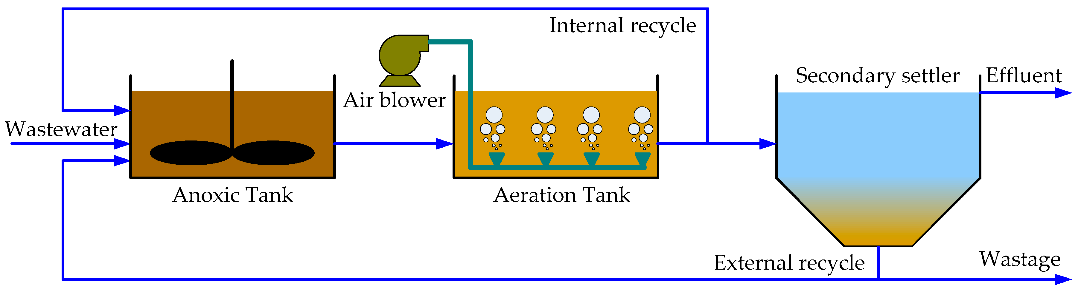
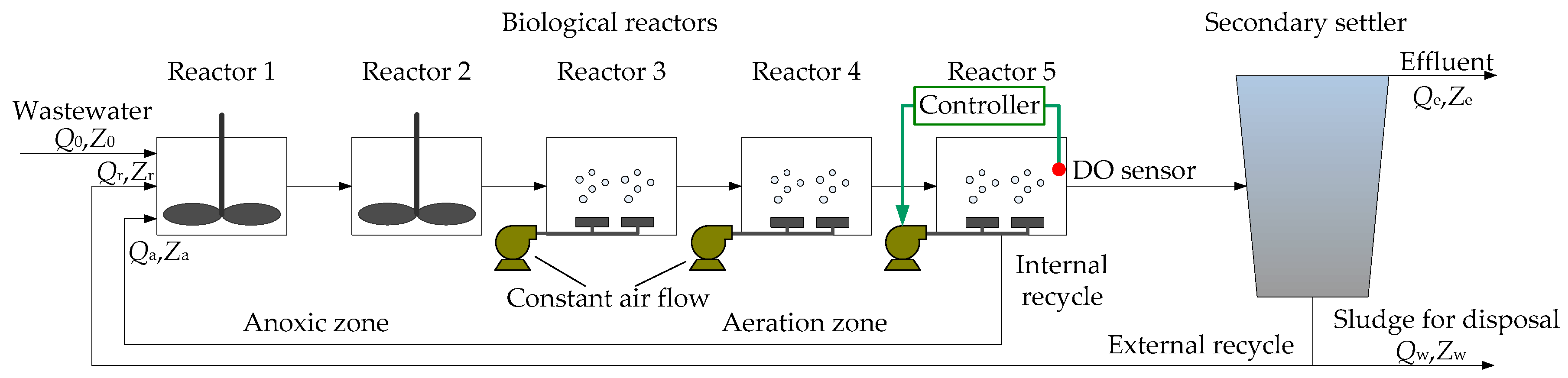
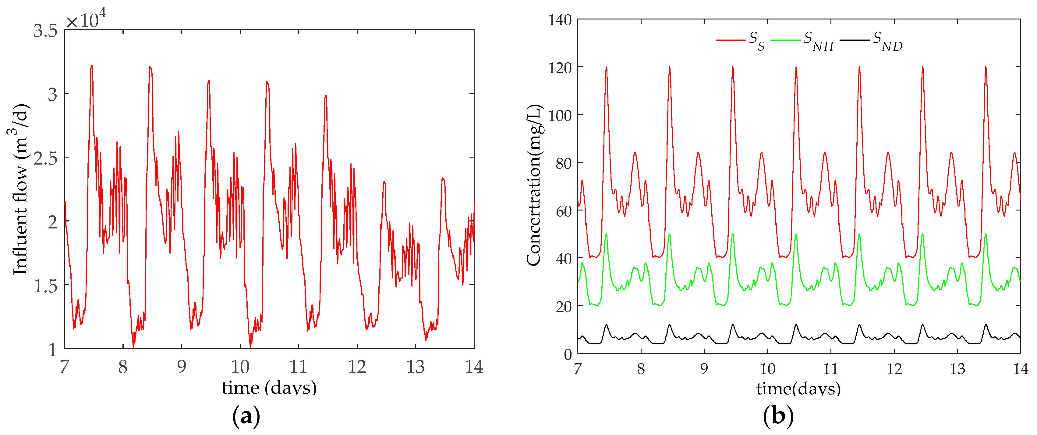
2.1. Activated Sludge Process (ASP) and Benchmark Simulation Model No. 1 (BSM1)

Activated sludge model No. 1 (ASM1) is a mathematical model that is widely accepted and applied in the research and application of activated sludge process (ASP) used in biological wastewater treatment systems. The typical ASP is shown in Figure 1, which includes two parts, the biological (more accurately biochemical) reaction tanks (or aeration tanks) and the secondary settler [27,28]. In the aeration tanks, the microorganisms are divided into active heterotrophic and autotrophic bacteria. The 13 reaction components and 8 reaction processes of the organic matter present in the influent are incorporated into the ASM1 [28,29,30]. In each process, all the organic substances and microorganisms have their own reaction rates and stoichiometry. Since the model has been published, researchers have been using the ASM1 model to verify their new proposed control algorithms of the DO concentration of ASP.
The activated sludge process aims to achieve, at minimum cost, sufficiently low concentrations of biodegradable matter and nutrients in the effluent together with minimal sludge production. In order to achieve this, the process has to be controlled [28]. However, it is difficult to predict the performance of the proposed or applied control strategy based on existing reference, process or location. To enhance the acceptance of innovative control strategies the performance evaluation should be based on a rigorous methodology that includes a simulation model, plant layout, controllers, performance criteria and test procedures.
The first Benchmark Simulation Layout (BSM1), which was based on the ASM1, is relatively a simple layout and is shown in Figure 2. Similar to ASM1, the first part of BSM1 is also a biological (or biochemical) activated sludge reactor, which is comprised of five-compartments, two of them are anoxic tanks and the following three are aerobic tanks; the second part of BSM1 is a secondary settler. Reactors 1 and 2 are unaerated in open-loop, but fully mixed; reactors 3, 4 and 5 are aerated. For the open-loop case, the oxygen transfer coefficients (KLa) are fixed; for reactors 3 and 4 the coefficient (KLa3 and KLa4) is set to a constant at 240 d−1 (10 h−1), which means the air flow rate of the blower is constant; for reactor 5, the coefficient (KLa5) is selected as the control variable (or operational variable) in this paper to be manipulated for maintaining the DO concentration at a level of 2mg/L. Thus, the system can achieve biological nitrogen removal through nitrification in the aeration tanks and pre-denitrification in the anoxic tanks. The model equations to be implemented for the proposed layout, the procedure to test the implementation and the performance criteria to be used are described below along with the description of sensors and control handles [28]. For more information, it can be seen in literature [28,29].
The ASM1 [27] has been selected to describe the biological phenomena taking place in the biological reactor and a double-exponential settling velocity function [31] has been selected to describe the secondary settler which is modeled as a 10 layers non-reactive unit (i.e., no biological reaction). In the activated sludge wastewater treatment system, the concentration of DO in the aeration tank is the most important parameter in the process of nitrogen removal [32]. Actually, the DO concentration has a direct impact on the effluent quality with respect to total nitrogen (Ntot), nitrate nitrogen (SNO) and ammonia (SNH). Therefore, the study of DO control has its important practical significance and prospect for application.
According to the mass balance of the system, the biochemical reactions that take place in each compartment (reactor) can be described as the follows.
Reactor 1
d Z 1 d t = 1 V 1 ( Q a Z a + Q r Z r + Q 0 Z 0 + r 1 V 1 Q 1 Z 1 )
Reactors 2 through 5 (k = 2 to 5)
d Z k d t = 1 V k ( Q k 1 Z k 1 + r k V k Q k Z k )
Special case for oxygen (SO,k)
d S O , k d t = 1 V k ( Q k 1 S O , k 1 Q k 1 S O , k ) ( K L a ) k ( S O * S O , k ) + r k
where, Q is the flow rate, Z is the mass concentration of either substrate or bacterial mass, V is the volume of the reactor, r is the reaction rate, KLa is the oxygen transfer coefficient, SO is the dissolved oxygen concentration. S* is the saturation concentration for oxygen (S* = 8 g/m3 at 15 °C); also Q1 = Qa + Qr + Q0; Qk = Qk−1.

2.2. A Neural Network Based Adaptive PID Algorithm

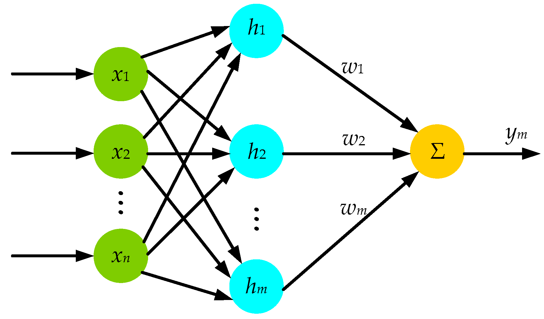
2.2.1. Radial Basis Function (RBF) Neural Network

Artificial neural network (ANN) is an artificial intelligence system to imitate biological neural networks (BNN). It uses nonlinear processing unit to simulate biological neurons for simulating the behavior of biological synapses among neurons by adjusting the variable weights between connected units. The specific topological structure of the network is organized from each processing unit in a certain connected form. Parallel processing ability and distributed storage are the main features of ANN. Furthermore, it has strong fault tolerance and nonlinear mapping ability with self-organization, self-learning and adaptive reasoning ability [33].
BP (backpropagation) network and RBF network are the most widely used forms of ANN. It is easily to be seen in the widely uses of pattern recognition, prediction, automatic control, etc. [34]. BP algorithm, a supervised learning algorithm, is based on gradient descent algorithm. The drawbacks of BP include an easy fall into local optimum, slow convergence speed, and disunity network structure. RBF network is a feedforward network based on the function approximation theory. It has strong global approximation ability, which can guarantee the network to approximation any kind of nonlinear function with arbitrary accuracy. It can fundamentally overcome the problem of local optimum occurs in BP network. The RBF network has the advantages of simple structure, fast convergence speed and strong generalization ability [35].
Radial basis function (RBF) neural network used in this paper is a three-layer forward network, which is a local approximation method of neural networks. The RBF neural network is composed of three layers, the input layer, the hidden layer and the output layer as shown in Figure 3. The mapping of the input layer to the output layer is nonlinear and the mapping of the space from the hidden layer to the output layer is linear. This kind of mapping configuration itself can speed up the learning rate and avoid the problem of local minima [18].
In Figure 3, the input vector of the input layer of the neural network is represented as:
X = [ x 1 , x 2 , , x s , , x n ] T
where, xs = [us(k), ys(k), ys(k − 1)], s = 1, 2, …, n; u(k) is the output of the controller; y(k) is the present (measured) output of the system (or process), that is, the measured value of DO concentration; y(k − 1) is the last measured value of DO concentration output from the process.
The middle layer is the hidden layer. The activation function of the hidden layer is composed of radial basis functions. Each array of computing units of hidden layers is called node. The radial basis vector of the nodes in the RBF neural network is shown in Equation (5).
T = [ h 1 , h 2 , , h j , , h m ] T
where, hj is Gaussian function,
h j = exp ( X C j 2 b j 2 )
where, j = 1, 2, …, m. Cj is the central vector of the first j node of the hidden layer of the RBF neural network,
C j = [ c j 1 , c j 2 , , c j i , , c j n ] T
where, i = 1, 2, …, n.
The basic width vector of the hidden layer node of the RBF neural network is
B = [ b 1 , b 2 , , b j , , b m ] T
where, bj is the parameter of the first j node and j = 1, 2, …, m.
The weight vector of RBF neural network W is given by:
W = [ w 1 , w 2 , , w j , , w m ] T
Then, the estimated output of the RBF network is defined as:
y m = w 1 h 1 + w 2 h 2 + + w m h m
The performance index function of the RBF neural network is set as follows:
E 1 = 1 2 ( y ( k ) y m ( k ) ) 2
where, y(k) is the system output and ym(k) is the estimated output of the RBF network.
From the above analysis, the three most important parameters C, W and B of a RBF neural network need to be obtained by the learning algorithm. In this paper, the gradient descent method is employed to obtain those three parameters of the nodes. The iterative algorithm used is as follows:
w j ( k ) = w j ( k 1 ) + η ( y ( k ) y m ( k ) ) h j + α ( w j ( k 1 ) w j ( k 2 ) )
Δ b j = ( y ( k ) y m ( k ) ) w j h j X C j 2 b j 3
b j ( k ) = b j ( k 1 ) + η Δ b j + α ( b j ( k 1 ) b j ( k 2 ) )
Δ c j i = ( y ( k ) y m ( k ) ) w j x j c j i b j 2
c j i ( k ) = c j i ( k 1 ) + η Δ c j i + α ( c j i ( k 1 ) c j i ( k 2 ) )
and the Jacobian matrix:
y ( k ) u ( k ) y m ( k ) u ( k ) = j = 1 m w j h j c j i x 1 b j 2
in which, η is the learning rate, α is the momentum factor and x1 = ∆u(k) is the control increment which is defined as the first input of the neural network.

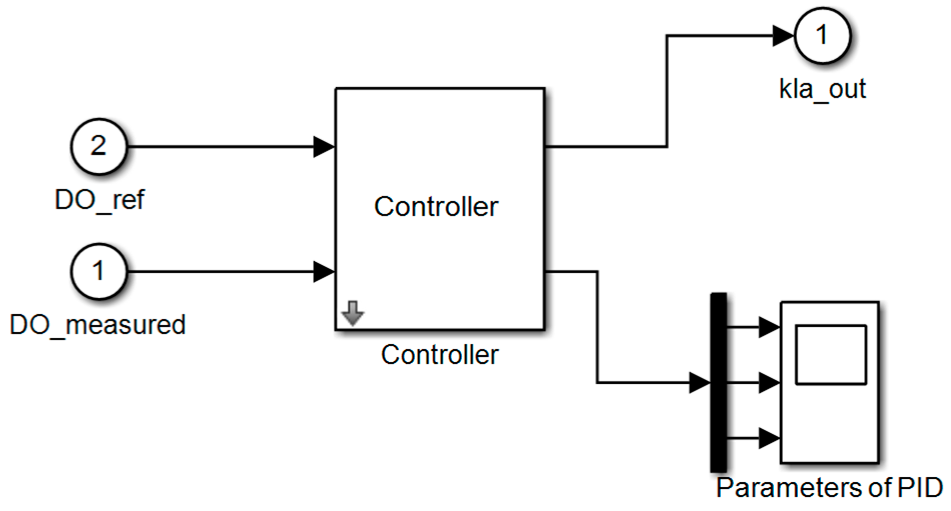
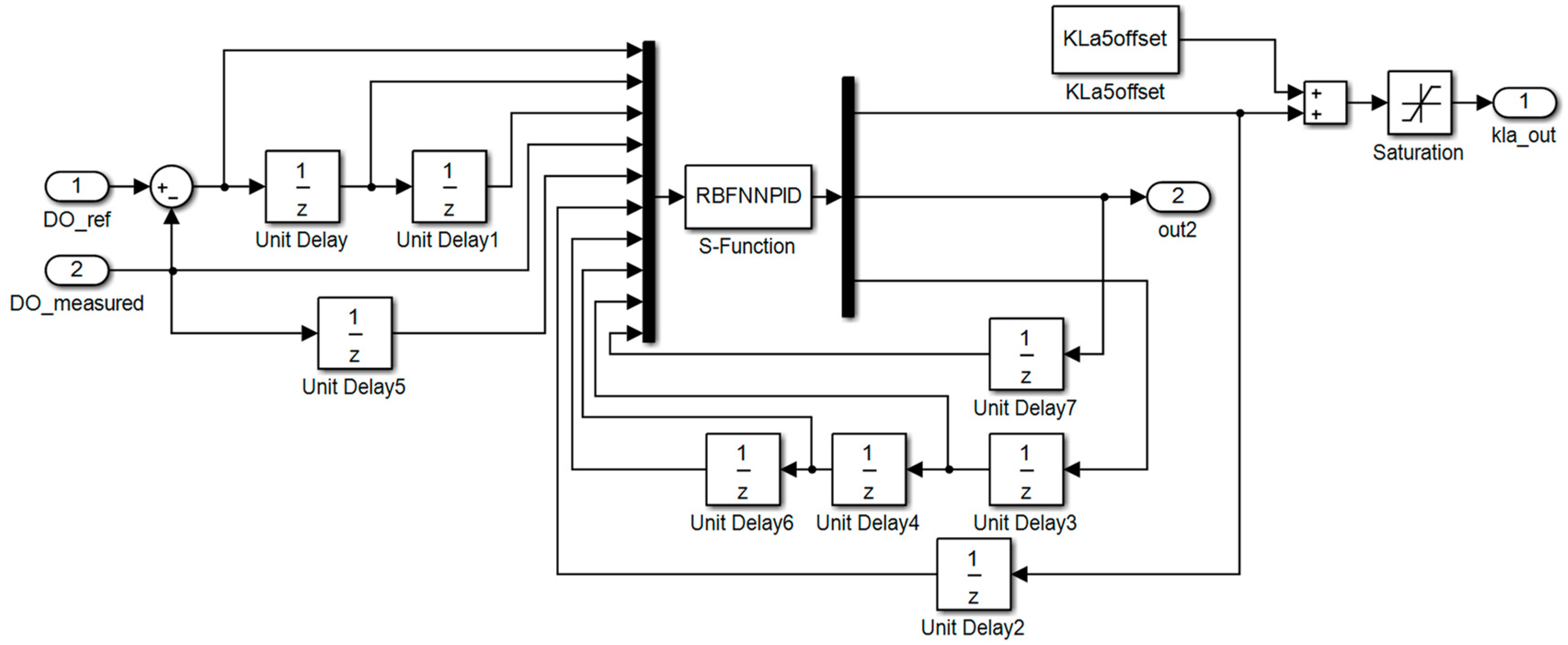
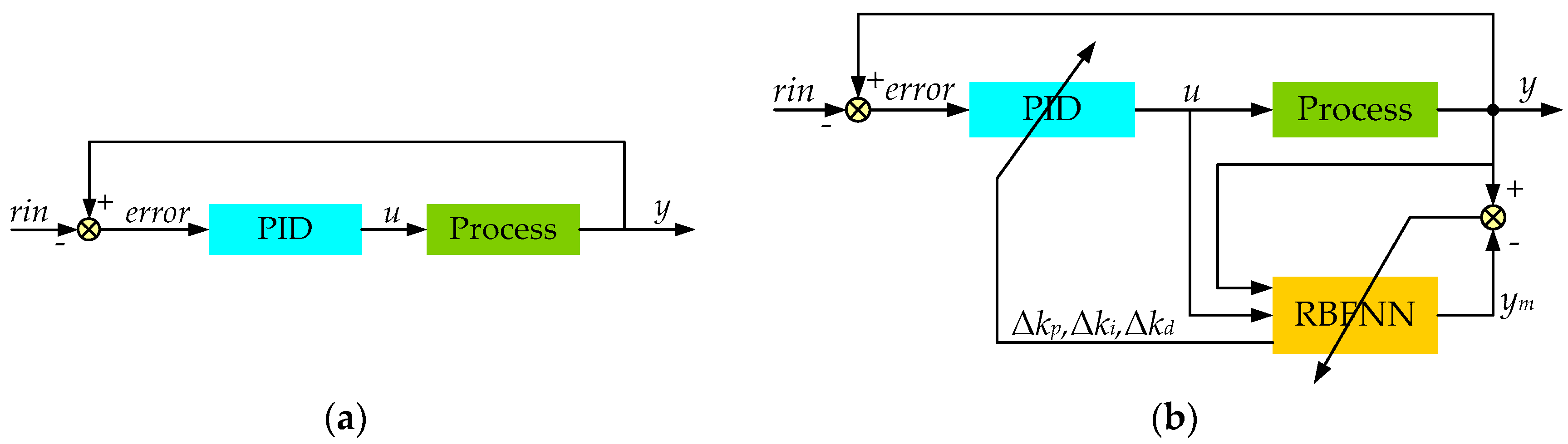
2.2.2. Design of the RBF Neural Network Based Adaptive PID (RBFNNPID) Algorithm

In the past decades, Proportional-Integral-Derivative (PID) is the main control method for DO level [36,37]. However, owing to the WWTP’s time-varying feature, strong nonlinearity, significant perturbations and large uncertainty, a fixed parameter linear controller is not able to maintain a satisfactory tracking performance under the full range of operating conditions [1,37].
The structure of the RBF neural network-based adaptive PID (RBFNNPID) algorithm is shown in Figure 4. The RBF neural network will adaptively calculate weighting coefficient and the parameter gradient information according to the operating state of the dissolved oxygen control system, by its own great learning ability. These results will be used to update the parameters of the PID controller in real time. Hence, such a repeated execution process realizes the adaptive adjustment of PID parameters and achieves the control of DO concentration.
We have adopted the incremental PID controller and the control error is:
e r r o r ( k ) = r i n ( k ) y ( k )
where, rin is the desired process value or setpoint of DO concentration; y(k) is the measured process value of DO.
The input of the PID algorithm is three errors, which are defined as:
x c ( 1 ) = e r r o r ( k ) e r r o r ( k 1 )
x c ( 2 ) = e r r o r ( k )
x c ( 3 ) = e r r o r ( k ) 2 e r r o r ( k 1 ) + e r r o r ( k 2 )
The output of the PID algorithm is:
u ( k ) = u ( k 1 ) + Δ u ( k )
Δ u ( k ) = k p x c ( 1 ) + k i x c ( 2 ) + k d x c ( 3 )
where, kp, ki and kd are the three parameters of the PID controller, which represents the proportion, integration and differentiation. The performance function is defined as:
E ( k ) = 1 2 ( e r r o r ( k ) ) 2
According to the gradient descent method, the adjustment rules of three parameters are given as:
Δ k p = η E k p = η E y y u u k p = η e r r o r ( k ) y u x c ( 1 )
Δ k i = η E k i = η E y y u u k i = η e r r o r ( k ) y u x c ( 2 )
Δ k d = η E k d = η E y y u u k d = η e r r o r ( k ) y u x c ( 3 )
in which, y / u is the identification information for the Jacobian matrix of the controlled object and it can be obtained through the identification process of neural network. The Jacobian matrix reflects the sensitivity of the output of the controlled object to the change of the input of the control.
The steps of the proposed RBFNNPID control strategy are as follows:
Step 1:
Initializing the network parameters, including the number of nodes in input layers and hidden layers, learning rate, inertia coefficient, the base width vector and the weight vector.
Step 2:
Sampling to get input rin and output y, calculating error in terms of Equation (18).
Step 3:
Calculating the output u of regulator according to Equation (22).
Step 4:
Calculating network output ym, adjusting center vector C, base width vector B, weight vector W and the Jacobian matrix in terms of Equations from (10) to (17) to obtain network identification information.
Step 5:
Adjusting parameters of regulator in terms of Equations (25)–(27).
Step 6:
Back to Step 2 and repeat the subsequent steps until the end of the simulation time.
The DO control module and the main codes of the S-function module of RBFNNPID can be found in Appendix A and Appendix B. Appendix C describes the stability and convergence analysis of the proposed RBFNNPID algorithm. An example to verify the convergence of the parameters of the neural network is shown in Appendix D.

3. Results

In order to verify the effectiveness and feasibility of the proposed neural network-based adaptive PID (RBFNNPID) algorithm for DO concentration control of the activated sludge wastewater treatment process, comparison simulation of RBFNNPID and traditional PID are designed in this section, including tracking performance and anti- disturbance performance.
We have selected the BSM1 as the simulation model and the dry weather wastewater data provided by IWA as the source data. The dry weather data contains two weeks long actual operational data of a wastewater treatment system, sampled at every 15 min. Figure 5 shows the dynamic influent data and the changes to the concentrations of some of the components between days 7 and 14.
In the simulation, the three parameters of both the traditional incremental PID algorithm and the proposed RBFNNPID algorithm are set as: kp = 5, ki = 1, kd = 0.5; the learning rate, η of the three parameters of PID is 0.2; the momentum factor α is 0.05; the network sampling period is 0.001 s; the structure of the RBFNN is defined as “3-6-1”, that is to say, the input layer has three nodes, the hidden layer has six nodes and the output layer has one node.

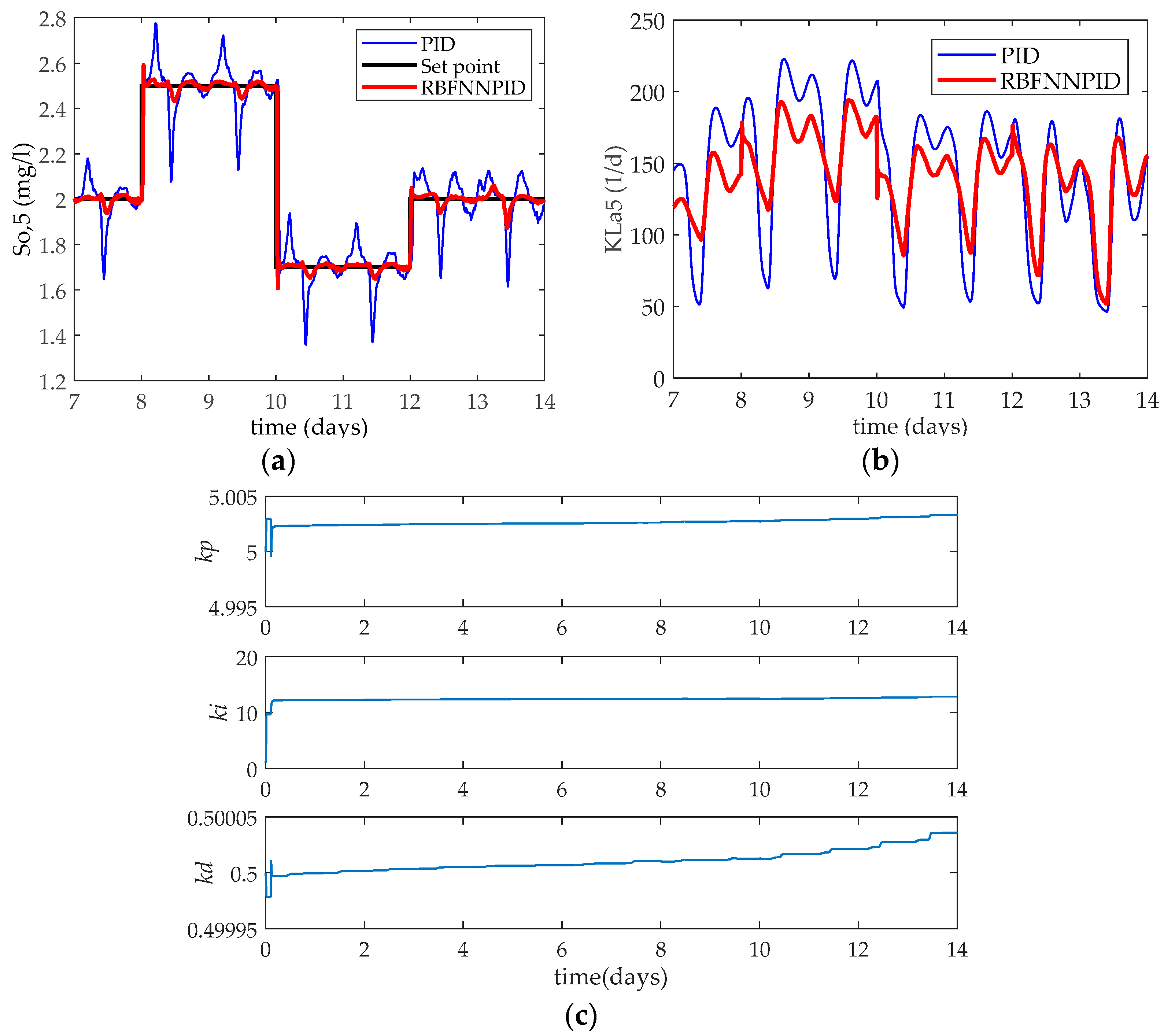
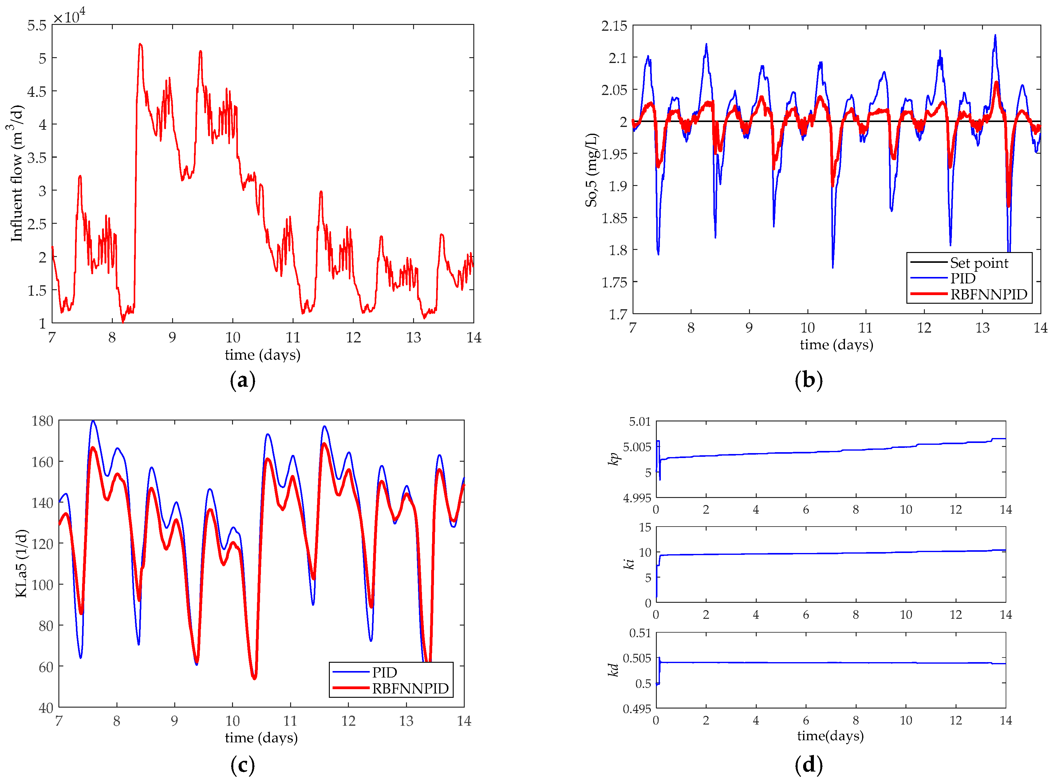
3.1. Tracking Performance Test 1

When the BSM1 wastewater treatment system is operating, due to the dynamic changes in the flow rate and composition of the influent, one need to adjust the oxygen transfer rate (KLa5) in the fifth tank in real-time to maintain the dissolved oxygen concentration in the appropriate range to ensure the effluent water quality meets the discharge standards. Therefore, how to control the DO concentration around the set point during the process is the aim of control algorithm that is being employed. The tracking performance is one of the deterministic criteria to evaluate whether an algorithm can be applied to an actual wastewater treatment system control.
Generally, the effluent water quality is the best when the DO concentration in the aeration tank is kept between 1~3 mg/L. Therefore, the DO concentration is setup to 2 mg/L in this simulation. The simulation results of last seven days are taken to evaluate the performance of the controller, which is shown in Figure 6.

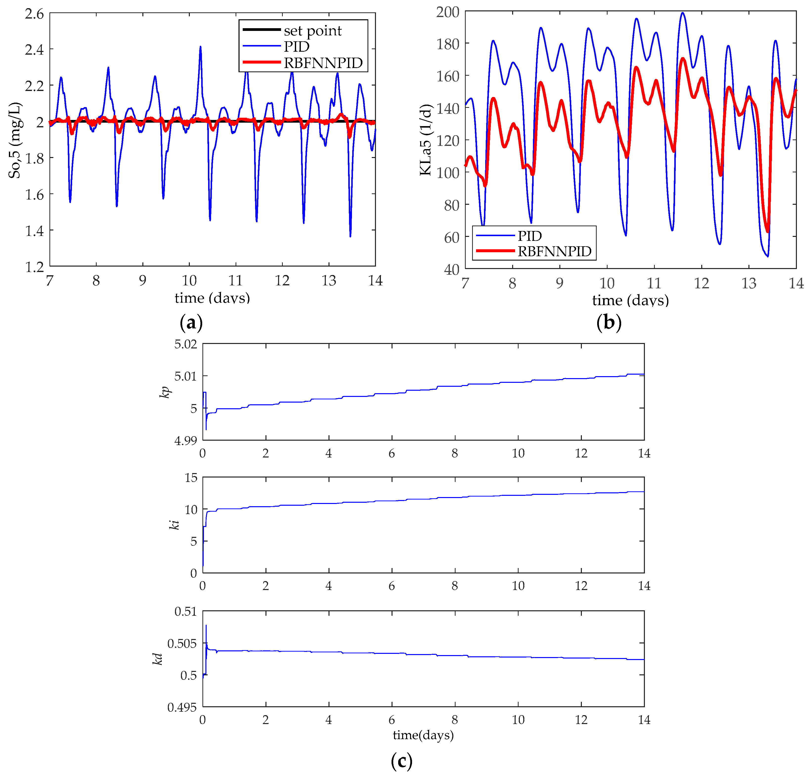
3.2. Tracking Performance Test 2

The set point of DO concentration was changed on days 8, 10 and 12 to 2.5, 1.7 and back to 2 mg/L, respectively to verify the tracking performance of the new proposed RBFNNPID algorithm. Simulation results are shown in Figure 7.

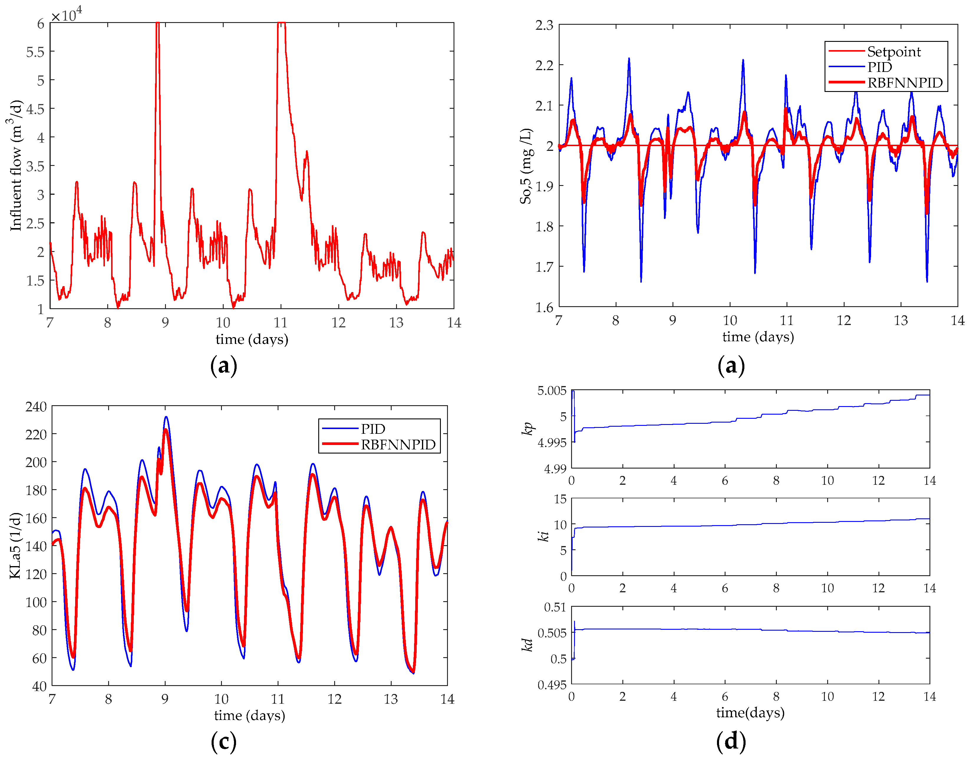
3.3. Anti-Disturbance Performance Test

A good control algorithm should not only have a good tracking performance, but also have a strong anti-disturbance ability. By having these properties, it can be applied to control a complex system such as wastewater treatment process to achieve a precise control effect. To further verify the anti-disturbance ability of the RBFNNPID algorithm, we used the data collected in rain and storm weather to simulate the algorithm. Different weather condition can be looked as different disturbances in the influent. The results are shown in Figure 8 and Figure 9.

3.4. Controller Performance Evaluation Index

There are two main indices for evaluating the performance of the dissolved oxygen controller. One is the assessment of the underlying control strategy. Indices include the integral of absolute error (IAE), the integral of squared error (ISE), the maximal deviation from set point (Devmax) and the variance of error (Vare). The four indices are calculated by Equation (28) through to (31) as shown below.
I A E i = t = 7 t = 14 | e i | d t
I S E i = t = 7 t = 14 e i 2 d t
D e v i max = max | e i |
V a r ( e i ) = I S E i T ( I A E i T ) 2
The aeration cost can be calculated using aeration energy (AE), which will be the economic indicator. AE is mainly used in the last three units of the biochemical reaction tanks. AE can be obtained by using the oxygen transfer function (KLa) of the three units as shown in Equation (32)
A E = S O * T · 1800 t = 7 t = 14 i = 1 i = 5 V i · K L a ( t ) d t
where, S O * is the saturation value of dissolved oxygen, Vi is the volume of each unit, and T is the calculation period of AE, in this case T = 7 days.
Generally, the smaller the value of the above evaluation indices, the better the performance of the controller is. Results of the evaluation indices are shown in Table 1 and Table 2. We can see that, under the different weather conditions, the RBFNNPID control strategy reduced the values of the above evaluation indices, compared with the traditional PID control strategy, indicating that the control performance of the system has been effectively improved, and the cost of aeration has also been reduced.

4. Discussion

PID may fail to achieve the control goal or effect of the process while using the traditional PID control algorithm due to unknown and unexpected disturbances as well as significant changes in operating conditions, such as a significant change in the (i) quality of influent; (ii) weather, etc. Therefore, in general, the parameters of the traditional PID controller need to be adjusted under different operating environments. However, a long period of accumulated experience and several tests are needed in order for the traditional PID to be adjusted to achieve satisfactory results under each operating environment. Clearly, it is not feasible in real time applications and increases the difficulty in applying it in different wastewater treatment plants. Our work will reduce the difficulty of parameter tuning of the traditional PID controller, which is essential to improve the adaptability of the PID control parameters in practice.
The simulation results in Figure 6a, Figure 7a, Figure 8b and Figure 9b show that the DO concentration is difficult to maintain at set point under the control of the conventional incremental PID controller when the influent flow rate and quality changed greatly. On the contrary, RBFNNPID can effectively maintain the DO concentration around the set value with a relatively low error by adjusting the air flow (which can be seen in Figure 6b, Figure 7b, Figure 8c and Figure 9c). It can be seen that the dynamic changes of the manipulated variable KLa5 is smooth under the control of RBFNNPID. This means we can get a more stable status by using less air supply to the aeration tank. Therefore, using RBFNNPID can reduce the aeration cost which is one of the major electrical costs of the wastewater treatment processes. It also can be verified from the results shown in Table 1 and Table 2.
According to the results of the rain weather and storm weather, which can be considered as there has the disturbances of the influent, shown in Figure 8 and Figure 9, compared with the conventional PID controller, the RBFNNPID controller can quickly and accurately track the desired output trajectory values, which means it not only has a good tracking performance, but also has a stronger anti-disturbance ability with the changes to the set points. Figure 6c, Figure 7c, Figure 8d and Figure 9d show the curves of the PID parameters are being adjusted adaptively. Parameters adjusted rapidly at the start of the simulation and small adjustments took place as the simulation goes on.
Applying precise control of the concentration of dissolved oxygen can not only avoid the occurrence of sludge bulking, but also reduce the aeration energy in a wastewater treatment plant. Intermittent aeration can be successfully implemented in a small-scale wastewater treatment plant to reduce the aeration energy while ensuring good effluent water quality [38]; however the same cannot be said in a large-scale wastewater treatment plant such as Pingliang Wastewater Treatment Plant that is situated in Gansu Province, China. In a large-scale wastewater treatment plant, intermittent aeration can reduce only a fraction of aeration energy. However, continuous aeration can effectively reduce the emissions of volatile organic compounds (VOCs) from a wastewater treatment plant, which has been proven as a factor for the increase of haze in some Chinese cities [39].
The characteristics of strong coupling, nonlinearity and large time delay of dissolved oxygen control system in activated sludge wastewater treatment and a control algorithm called RBFNNPID algorithm are discussed in this paper. However, this algorithm has not been applied directly into practice so far as it has certain complexity. We are currently undertaking the following two studies to verify its feasibility, validity, and superiority: (i) Simplifying the algorithm for practical use; (ii) Trialing the algorithm at Pingliang Wastewater Treatment Plant in Gansu Province, China.

5. Conclusions

In this paper, an adaptive PID control algorithm based on RBF neural network is proposed. The RBFNNPID algorithm combines the good learning and adaptive ability of neural networks and the practical advantages of PID algorithm. The gradient descent method is used to adaptively adjust the increment of the three parameters of the PID controller to achieve an optimal control effect on the control of DO concentration. The simulation results show that the RBFNNPID algorithm not only has a better performance of tracking and anti-jamming, but also has a great improvement to the robustness compared to that of the traditional PID. Thus, it can reduce the aeration costs of a wastewater treatment plant employing ASP.

Acknowledgments

China Scholarship Council (CSC) supported the first author to visit RMIT University as visiting scholar while undertaking this work. This work is also supported by the other funding include the National Natural Science Foundation of China (No. 61563032), the Natural Science Foundation of Gansu province (No. 1506RJZA104), University Scientific Research Project of Gansu province (No. 2015B-030), and the Excellent Young Teacher Project of Lanzhou University of Technology (No. Q201408).

Author Contributions

Xianjun Du, Guohua Shi and Junlu Wang conceived and designed the experiments; Junlu Wang performed the experiments; Xianjun Du, Junlu Wang and Veeriah Jegatheesan analyzed the data; Xianjun Du and Veeriah Jegatheesan wrote the paper.

Conflicts of Interest

The authors declare no conflict of interest.

Appendix A

We designed a DO control module in the Matlab Simulink environment which is shown in Figure A1. The output one “kla_out” is used to adjust the air flow of the blower, equipped for reactor 5, to maintain the DO concentration at a level of desired value. The scope is used to monitor the dynamic changes of the three parameters of the controller, which have been shown in Figure 6c, Figure 7c, Figure 8d and Figure 9d. Detail of the inner structure of the controller is shown in Figure A2.
Figure A1. Overview of the DO control module.
Applsci 08 00261 g0a1
Figure A2. Detailed structure of the RBFNNPID controller.
Applsci 08 00261 g0a2

Appendix B

The main codes of the S-function module, shown in Figure A2, are given below:
function [sys, x0, str, ts] = nnrbf_pid(t,x,u,flag,T,nn,K_pid, eta_pid, xite, alfa, beta0, w0)
  switch flag,
    case 0, [sys, x0, str, ts] = mdlInitializeSizes(T,nn);
    case 2, sys = mdlUpdates(u);
    case 3, sys = mdlOutputs(t, x, u, T,nn, K_pid,eta_pid, xite, alfa, beta0, w0);
    case {1, 4, 9}, sys = [];
    otherwise, error (['Unhandled flag = ' , num2str(flag)]);
  end
function [sys,x0,str,ts] = mdlInitializeSizes(T, nn)
  sizes = simsizes;
  sizes. NumContStates = 0;
  sizes.NumDiscStates = 3;
  sizes. NumOutputs = 4 + 5* nn;
  sizes.NumInputs = 9 + 15* nn;
  sizes. DirFeedthrough = 1;
  sizes. NumSampleTimes =1;
  sys = simsizes(sizes) ;
  x0 = zeros(3, 1);
  str = [];
  ts = [T0];
function sys = mdlUpdates(u)
  sys = [ u(1) − u(2); u(1); u(1) + u(3) − 2* u(2)];
function sys = mdlOutputs(t, x, u,T, nn, K_pid, eta_pid, xite, alfa, beta0, w0)
  % Initialization of the radial basis centers
  ci3 = reshape(u(7: 6 + 3* nn), 3, nn);
  ci2 = reshape(u(7 + 5* nn: 6 + 8* nn), 3, nn);
  ci1 = reshape(u(7 + 10* nn: 6 + 13* nn), 3, nn);
  % Initialization of the radial basis width
  bi3 = u(7 + 3* nn: 6 + 4* nn);
  bi2 = u(7 + 8*nn: 6 + 9* nn);
  bi1 = u(7 + 13* nn: 6 + 14* nn);
  % Initialization of the weights
  w3 = u(7 + 4* nn: 6+ 5* nn) ;
  w2 = u(7 + 9* nn: 6+ 10* nn) ;
  w1 = u(7 + 14* nn: 6+ 15* nn) ;
  xx = u([6; 4; 5]);
  if t = 0
    % Initialize the PID parameters
    ci1 = w0(1) * ones(3, nn);
    bi1 = w0(2) *ones(nn, 1);
    w1 = w0(3) * ones(nn, 1);
    K_pid0 = K_pid;
    else
    % Update the PID parameters
    K_pid0 = u(end-2: end);
  end
  for j = 1: nn
    % Gaussian
    h(j, 1) = exp(−norm(xx−ci1( : , j))^2/(2* bi1(j) * bi1(j)));
  end
  % Dynamic of gradient descent method
  dym = u(4) − w1'* h;
  W = w1 + xite* dym* h + alfa* (w1 − w2) + beta0*(w2 − w3) ;
  for j = 1: nn
    dbi(j,1) = xite* dym* w1(j) * h(j) * (bi1(j) ^(−3)) * norm(xx − ci1(:,j))^2;
    dci( : ,j) = xite*dym* w1(j)* h(j) * (xx − ci1(:,j)) * (bi1(j)^(−2));
  end
  bi = bi1 + dbi + alfa* (bi1 − bi2) + beta0*(bi2 − bi3) ;
  ci = ci1 + dci + alfa* (ci1 − ci2) + beta0*(ci2 − ci3) ;
  % Jacobian
  dJac = sum(w.*h.*(−xx (1) + ci (1,:)') ./bi.^2);
  % adjustments of the PID parameters
  KK(1) = K_pid0(1) + u(1) * dJac* eta_pid(1)* x(1);
  KK(2) = K_pid0(2) + u(1) * dJac* eta_pid(2)* x(2);
  KK(3) = K_pid0(3) + u(1) * dJac* eta_pid(3)* x(3);
  sys= [ u(6) + KK* x; KK'; ci( : ) ; bi( : ) ; w( : ) ] ;

Appendix C

This section describes the stability and convergence analysis of the proposed RBFNNPID algorithm.
The basic knowledge of the stability and convergence analysis is Lyapunov theorem, also known as Lyapunov stability.
V ( x 1 , x 2 , K , x N ) is an arbitrary function defined in the neighborhood of the origin Ω, where Ω is a state of equilibrium and x 1 , x 2 , K , x N are variables, then
| x i | H , i = 1 , 2 , K , N
where, H is a positive constant.
Assuming that V is a continuous differentiable function in Ω and V ( 0 , 0 , K , 0 ) = 0 . Such that
(i)
V(x) > 0 is positive definite or V(x) < 0 is negative definite, x ∈ Ω and x ≠ 0;
(ii)
V(x) > 0 is positive semi-definite or V(x) < 0 is negative semidefinite, x ∈ Ω;
Consider an autonomous nonlinear dynamical system
x ˙ = f ( x )
where, f(0) = 0.
Assuming xi = xi(t), (i = 1, 2, K, N) is the solution of the system (A2). We can obtain the derivation
d V d t = V x 1 x 1 t + V x 2 x 2 t + K + V x N x N t
Introducing the gradient vector (Equation (A4)) into Equation (A3)
V ( x ) = [ V x 1 , V x 2 , L , V x N ] T
We will arrive at the final equation as below:
V = [ V ( x ) ] T f ( x ) = ω ( x )
The following conclusions can be made from the above analysis:
(i)
If V(x) is positive (or negative) definite, and if derivation V = ω ( x ) is negative (or positive) semi-definite, the system is said to be Lyapunov stable at the equilibrium of the origin;
(ii)
If V(x) is positive (or negative) definite, and if derivation V = ω ( x ) is negative (or positive) definite, the system is said to be exponentially stable at the equilibrium of the origin;
(iii)
If V(x) is positive (or negative) definite, and if derivation V = ω ( x ) is also positive (or negative) definite, the system is said to be unstable at the equilibrium of the origin;
For the adjustment of the weights of the neural network, we need a parameter called learning rate η. If η is too large, NN will be unstable; but if η is too small, the convergence rate will be too slow. Therefore, the selection of the value of learning rate is crucial to the stability and convergence of the system.
Assuming the indicator function of the RBFNNPID controller
J ( k ) = 1 2 [ y ( k ) y m ( k ) ] 2 = 1 2 e 2 ( k )
where, e(k) is the learning error of the network.
In order to ensure the adjustment of the weight coefficient is carried out in the direction of the negative gradient relative to ω(k), there must be
ω ( k + 1 ) = ω ( k ) η J ( k ) ω ( k )
From Equations (A6) and (A7), we can get
Δ ω ( k ) = J ( k ) ω ( k ) = e ( k ) e ( k ) ω ( k ) = e ( k ) e ( k ) Δ u ( k ) Δ u ( k ) ω ( k )
Defining a Lyapunov function of a discrete-time systems as
v ( k ) = 1 2 e 2 ( k )
As we introduced in the paper, the gradient descent method is used as the change of the network-learning algorithm.
Δ v ( k ) = v ( k + 1 ) v ( k ) = 1 2 e 2 ( k + 1 ) 1 2 e 2 ( k ) = 1 2 Δ e ( k ) [ 2 e ( k ) + Δ e ( k ) ]
where, e(0) = 0, and,
Δ e ( k ) = J ( k ) e ( k ) = e ( k )
It can be obtained from Equation (A8), that
Δ e ( k ) = e ( k ) = ( e ( k ) ω ( k ) ) T Δ ω ( k )
and
Δ ω ( k ) = η J ( k ) ω ( k ) = η e ( k ) e ( k ) Δ u ( k ) Δ u ( k ) ω ( k )
By substituting Equation (A13) into Equation (A12)
Δ e ( k ) = η J ( k ) ω ( k ) 2 e ( k )
Then, substituting Equation (A14) into Equation (A10)
Δ v ( k ) = 1 2 η J ( k ) ω ( k ) 2 e ( k ) [ 2 e ( k ) η J ( k ) ω ( k ) 2 e ( k ) ] = 1 2 η J ( k ) ω ( k ) 2 e 2 ( k ) [ 2 η J ( k ) ω ( k ) 2 ]
Knowing from the Lyapunov stability theory, the system is stable when Δ v < 0 . In addition, because of η > 0 ,
2 η J ( k ) ω ( k ) 2 > 0
That is,
0 < η < 2 J ( k ) ω ( k ) 2
Therefore, the system is stable.
When Δ v < 0 ,
1 2 e 2 ( k + 1 ) < 1 2 e 2 ( k )
lim k e ( k ) = 0
It means, with the increase of k, e(k) gradually reaches to zero, and it guarantees the convergence of the learning algorithm. Based on the above analysis, if the value of η is according to Equation (A17), the system is stable and the learning algorithm will converge.

Appendix D

To verify the convergence of the parameters of the neural network, the dynamic changes of the centers (Figure A3) as well as weights and widths (Figure A4) of the neural network were computed, taking the first neuron of the hidden layer neurons as the example. From those figures, it can be seen that the parameters are converging with adaptive changes while the control process is going on.
Figure A3. Dynamic changes of the centers of the first neuron (of the hidden layer neurons) of the neural network. (Where, ×1, ×2 and ×3 represent the three centers of the first neuron).
Applsci 08 00261 g0a3
Figure A4. Dynamic changes of the weights and widths of the first neuron (of the hidden layer neurons) of the neural network.
Applsci 08 00261 g0a4

References

  1. Bo, Y.C.; Zhang, X. Online adaptive dynamic programming based on echo state networks for dissolved oxygen control. Appl. Soft Comput. 2017. [Google Scholar] [CrossRef]
  2. Holenda, B.; Domokos, E.; Rédey, Á.; Fazakas, J. Dissolved oxygen control of the activated sludge wastewater treatment process using model predictive control. Comput. Chem. Eng. 2008, 32, 1270–1278. [Google Scholar] [CrossRef]
  3. Zhang, P.; Yuan, M.; Wang, H. Study on Dissolved Oxygen Control Method Based on International Evaluation Benchmark. Inf. Control 2007, 36, 199–203. [Google Scholar]
  4. Yu, K.; Muhetaer, A.; Wei, L. Evaluation indexes of sewage stabilization from municipal wastewater treatment plant. China Water Wastewater 2016, 5, 93–97. [Google Scholar]
  5. Chen, C.S. Robust self-organizing neural-fuzzy control with uncertainty observer for MIMO nonlinear systems. IEEE Trans. Fuzzy Syst. 2011, 19, 694–706. [Google Scholar] [CrossRef]
  6. Nascu, I.; Vlad, G.; Folea, S.; Buzdugan, T. Development and application of a PID auto-tuning method to a wastewater treatment process. In Proceedings of the IEEE International Conference on Automation, Quality and Testing, Robotics (AQTR 2008), Cluj-Napoca, Romania, 22–25 May 2008. [Google Scholar]
  7. Ye, H.T.; Li, Z.Q.; Luo, W.G. Dissolved oxygen control of the activated sludge wastewater treatment process using adaptive fuzzy PID control. In Proceedings of the 32nd Chinese Control Conference (CCC2013), Xi’an, China, 26–28 July 2013. [Google Scholar]
  8. Goldar, A.; Revollar, S.; Lamanna, R.; Vega, P. Neural-MPC for N-removal in activated-sludge plants. In Proceedings of the IEEE European Control Conference (ECC 2014), Strasbourg, France, 24–27 June 2014. [Google Scholar]
  9. Goldar, A.; Revollar, S.; Lamanna, R.; Vega, P. Neural NLMPC schemes for the control of the activated sludge process. In Proceedings of the 11th IFAC Symposium on Dynamics and Control of Process Systems Including Biosystems, Trondheim, Norway, 6–8 June 2016. [Google Scholar]
  10. Belchior, C.A.C.; Araújo, R.A.M.; Landeck, J.A.C. Dissolved oxygen control of the activated sludge wastewater treatment process using stable adaptive fuzzy control. Comput. Chem. Eng. 2012, 37, 152–162. [Google Scholar] [CrossRef]
  11. Jeppsson, U.; Rosen, C.; Alex, J.; Copp, J.; Gernaey, K.V.; Pons, M.N.; Vanrolleghem, P.A. Towards a benchmark simulation model for plant-wide control strategy performance evaluation of WWTPs. Water Sci. Technol. 2006, 53, 287–295. [Google Scholar] [CrossRef] [PubMed]
  12. Yu, G.; Zhang, P.; Wei, S.; Fan, M.; Wang, H. Human-simulation intelligent PID control theory and its application for dissolved oxygen in wastewater treatment. Microcomput. Inf. 2006, 22, 13–15. [Google Scholar]
  13. Syu, M.J.; Chen, B.C. Back-propagation neural network adaptive control of a continuous wastewater treatment process. Ind. Eng. Chem. Res. 1998, 37, 3625–3630. [Google Scholar] [CrossRef]
  14. Macnab, C.J.B. Stable Neural-Adaptive Control of Activated Sludge Bioreactors. In Proceedings of the 2014 American Control Conference (ACC2014), Portland, OR, USA, 4–6 June 2014. [Google Scholar]
  15. Mirghasemi, S.; Macnab, C.J.B.; Chu, A. Dissolved oxygen control of activated sludge bioreactors using neural-adaptive control. In Proceedings of the IEEE Symposium on Computational Intelligence in Control and Automation (CICA 2014), Orlando, FL, USA, 9–12 December 2014. [Google Scholar]
  16. Ruan, J.; Zhang, C.; Li, Y.; Li, P.; Yang, Z.; Chen, X.; Huang, M.; Zhang, T. Improving the efficiency of dissolved oxygen control using an on-line control system based on a genetic algorithm evolving FWNN software sensor. J. Environ. Manag. 2017, 187, 550–559. [Google Scholar] [CrossRef] [PubMed]
  17. Qiao, J.; Fu, W.; Han, H. Dissolved oxygen control method based on self-organizing T-S fuzzy neural network. CIESC J. 2016, 67, 960–966. [Google Scholar]
  18. Li, M.; Zhou, L.; Wang, J. Neural network predictive control for dissolved oxygen based on Levenberg-Marquardt algorithm. Trans. Chin. Soc. Agric. Mach. 2016, 47, 297–302. [Google Scholar]
  19. Xu, J.; Yang, C.; Qiao, J. A novel dissolve oxygen control method based on fuzzy neural network. In Proceedings of the 36th Chinese Control Conference (CCC2017), Dalian, China, 26–28 July 2017. [Google Scholar]
  20. Lin, M.J.; Luo, F. Adaptive neural control of the dissolved oxygen concentration in WWTPs based on disturbance observer. Neurocomputing 2016, 185, 133–141. [Google Scholar] [CrossRef]
  21. Han, H.G.; Qiao, J.F.; Chen, Q.L. Model predictive control of dissolved oxygen concentration based on a self-organizing RBF neural network. Control Eng. Pract. 2012, 20, 465–476. [Google Scholar] [CrossRef]
  22. Zhou, H. Dissolved oxygen control of wastewater treatment process using self-organizing fuzzy neural network. CIESC J. 2017, 68, 1516–1524. [Google Scholar]
  23. Huang, M.Z.; Han, W.; Wan, J.Q.; Chen, X. Multi-objective optimization for design and operation of anaerobic digestion using GA-ANN and NSGA-II. J. Chem. Technol. Biotechnol. 2016, 91, 226–233. [Google Scholar] [CrossRef]
  24. Li, Y.; Li, T.; Jiang, Y.; Fan, J.-L. Adaptive PID control of quadrotor based on RBF neural network. Control Eng. China 2016, 23, 378–382. [Google Scholar]
  25. Chamsai, T.; Jirawattana, P.; Radpukdee, T. Robust adaptive PID controller for a class of uncertain nonlinear systems: An application for speed tracking control of an SI engine. Math. Probl. Eng. 2015, 17, 1–12. [Google Scholar] [CrossRef]
  26. Lin, C.M.; Chung, C.C. Fuzzy brain emotional learning control system design for nonlinear systems. Int. J. Fuzzy Syst. 2015, 17, 117–128. [Google Scholar] [CrossRef]
  27. Henze, M.; Grady, C.P.L.; Gujer, W.; Matsuo, T. Activated Sludge Model No. 1; IAWPRC Publishing: London, UK, 1987. [Google Scholar]
  28. Gernaey, K.V.; Jeppsson, U.; Vanrolleghem, P.A.; Copp, J.B. Benchmarking of Control Strategies for Wastewater Treatment Plants; IWA Publishing: London, UK, 2014. [Google Scholar]
  29. Du, X.J.; Hao, X.H.; Li, H.J.; Ma, Y.W. Study on modelling and simulation of wastewater biochemical treatment activated sludge process. Asian J. Chem. 2011, 23, 4457–4460. [Google Scholar]
  30. Simsek, H. Mathematical modeling of wastewater-derived biodegradable dissolved organic nitrogen. Environ. Technol. 2016, 37, 2879–2889. [Google Scholar] [CrossRef] [PubMed]
  31. Takács, I.; Patry, G.G.; Nolasco, D. A dynamic model of the clarification thickening process. Water Res. 1991, 25, 1263–1271. [Google Scholar] [CrossRef]
  32. Olsson, G.; Newell, B. Wastewater Treatment Systems: Modelling, Diagnosis and Control, 1st ed.; IWA Publishing: London, UK, 1999. [Google Scholar]
  33. Maier, H.R.; Dandy, G.C. Neural networks for the prediction and forecasting of water resources variables: A review of modelling issues and applications. Environ. Model. Softw. 2000, 15, 101–124. [Google Scholar] [CrossRef]
  34. Wang, J.; Shi, P.; Jiang, P.; Xiao, P. Application of BP Neural Network Algorithm in Traditional Hydrological Model for Flood Forecasting. Water 2017, 9, 48. [Google Scholar] [CrossRef]
  35. Zebardast, B.; Maleki, I. A New Radial Basis Function Artificial Neural Network based Recognition for Kurdish Manuscript. Int. J. Appl. Evolut. Comput. 2013, 4, 72–87. [Google Scholar] [CrossRef]
  36. Wahab, N.A.; Katebi, R.; Balderud, J. Multivariable PID control design for activated sludge process with nitrification and denitrification. Biochem. Eng. J. 2009, 45, 239–248. [Google Scholar] [CrossRef]
  37. Luo, F.; Hoang, B.L.; Tien, D.N.; Nguyen, P.H. Hybrid PI controller design and hedge algebras for control problem of dissolved oxygen in the wastewater treatment system using activated sludge method. Int. Res. J. Eng. Technol. 2015, 2, 733–738. [Google Scholar]
  38. Sánchezmonedero, M.A.; Aguilar, M.I.; Fenoll, R.; Roig, A. Effect of the aeration system on the levels of airborne microorganisms generated at wastewater treatment plants. Water Res. 2008, 42, 3739–3744. [Google Scholar] [CrossRef] [PubMed]
  39. Chen, W.H. Influences of Aeration and Biological Treatment on the Fates of Aromatic VOCs in Wastewater Treatment Processes. Aerosol Air Qual. Res. 2013, 13, 225–236. [Google Scholar] [CrossRef]
Figure 1. Typical biological (or biochemical) ASP to treat wastewater. ASP: Activated Sludge Process.
Applsci 08 00261 g001
Figure 2. Schematic representation of Benchmark Simulation Model No. 1 (BSM1) model.
Applsci 08 00261 g002
Figure 3. Topology of a radial basis function (RBF) neural network.
Applsci 08 00261 g003
Figure 4. Block diagram comparing two controllers: (a) Block diagram of a traditional PID controller in a feedback loop; (b) Block diagram of proposed RBF neural network-based adaptive PID (RBFNNPID) controller. PID: Proportional-Integral-Derivative.
Applsci 08 00261 g004
Figure 5. Dynamic data for experimental use: (a) Influent flow rate (days 7 to 14); (b) Concentration of some of the chemical species in the influent (days 7 to 14) (SS—readily biodegradable substrate; SNH—ammonium and ammonia nitrogen; SND—soluble biodegradable organic nitrogen).
Applsci 08 00261 g005
Figure 6. Comparison results of the tracking performance (dry weather): (a) DO concentration in the fifth tank; (b) Dynamic changes of the manipulated variable KLa5; (c) Dynamic adaptive adjustments of the three parameters kp, ki, kd of RBFNNPID algorithm.
Applsci 08 00261 g006
Figure 7. Comparison results of the tracking performance (changing set point of DO): (a) DO concentration in the fifth tank; (b) Dynamic changes of the manipulated variable KLa5; (c) Dynamic adaptive adjustments of the three parameters kp, ki, kd of RBFNNPID algorithm.
Applsci 08 00261 g007
Figure 8. Comparison results of the anti-disturbance performance (rain weather): (a) Influent flow rate (days 7 to 14); (b) DO concentration in the fifth tank; (c) Dynamic changes of the manipulated variable KLa5; (d) Dynamic adaptive adjustments of the three parameters kp, ki, kd of RBFNNPID algorithm.
Applsci 08 00261 g008
Figure 9. Comparison results of the anti-disturbance performance (storm weather): (a) Influent flow rate (days 7 to 14); (b) DO concentration in the fifth tank; (c) Dynamic changes of the manipulated variable KLa5; (d) Dynamic adaptive adjustments of the three parameters kp, ki, kd of RBFNNPID algorithm.
Applsci 08 00261 g009
Table 1. Performance of two DO control methods.
WeatherMethodISEIAEDevmaxVare
DryRBFNNPID1.64× 10−22.08× 1011.89× 1012.10× 103
PID4.44× 10−24.03× 1013.43× 1016.30× 103
RainRBFNNPID2.50× 1039.47× 10−26.94× 10−23.53× 104
PID3.59× 10−23.61× 1012.95× 1015.10× 103
StormRBFNNPID5.70× 1031.39× 1011.46× 1018.16× 104
PID1.38× 10−22.27× 1011.97× 1012.00× 103
Table 2. Aeration energy of two control methods.
WeatherPID (kWh/d)RBFNNPID (kWh/d)
Dry7149.97032.1
Rain6955.86805.8
Storm7199.66971.8

