Progress in Forward-Inverse Modeling Based on Radiative Transfer Tools for Coupled Atmosphere-Snow/Ice-Ocean Systems: A Review and Description of the AccuRT Model

Abstract

A tutorial review is provided of forward and inverse radiative transfer in coupled atmosphere-snow/ice-water systems. The coupled system is assumed to consist of two adjacent horizontal slabs separated by an interface across which the refractive index changes abruptly from its value in air to that in ice/water. A comprehensive review is provided of the inherent optical properties of air and water (including snow and ice). The radiative transfer equation for unpolarized as well as polarized radiation is described and solutions are outlined. Several examples of how to formulate and solve inverse problems encountered in environmental optics involving coupled atmosphere-water systems are discussed in some detail to illustrate how the solutions to the radiative transfer equation can be used as a forward model to solve practical inverse problems.

1. Introduction

Reliable, accurate, and efficient modeling of electromagnetic radiation transport in turbid media has important applications in studies of Earth’s climate by remote sensing. For example, such modeling is needed to develop forward-inverse methods used to quantify types and concentrations of aerosol and cloud particles in the atmosphere, as well as dissolved organic and particulate biogeochemical matter in lakes, rivers, coastal water, and open-ocean water, and to simulate the performance of remote sensing detectors deployed on aircraft, balloons, and satellites. Accurate radiative transfer (RT) modeling is also required to compute irradiances and scalar irradiances that are used to compute warming/cooling and photolysis rates in the atmosphere, solar energy deposition in the cryosphere including frozen fresh water (lakes and rivers), sea ice, and glaciers, as well as primary production rates in the water. Finally, RT modeling is needed to compute the Stokes vector describing the polarization state of the radiation field, which is desired in many remote sensing applications.

Accurate, efficient, and easy-to-use radiative transfer (RT) simulation tools are important because they (i) can be used to generate irradiances as well as total and polarized radiances (including degree of polarization) at any location and direction; (ii) will provide accurate results for given input parameters and specified inherent optical properties (IOPs); (iii) will lead to significant progress in research areas such as remote sensing algorithm development, climate research, and other atmospheric and hydrologic applications.

Available tools for atmospheric applications include: (i) SBDART [1], Streamer [2], and LibRadtran (www.libradtran.org), which all apply to the atmosphere only; there is no coupling to an underlying surface consisting of e.g., solid (snow/ice) or liquid water; (ii) Hydrolight, which applies to water only, provides water-leaving radiance, but not top-of-the-atmosphere (TOA) radiance; there is no coupling to the atmosphere (assumed to be a boundary condition). To remedy this situation a new Accurate Radiative Transfer (AccuRT) tool was developed to facilitate well-tested and robust RT simulations in coupled systems consisting of two slabs with different refractive indices. Please note that we here use the word “water” generically to describe the solid phase (i.e., snow and ice) as well as the liquid phase. The AccuRT tool accounts for reflection and transmission at the interface between the two slabs, and allows each slab to be divided into a sufficient number of layers to resolve the variation in the IOPs with depth.

Notation

Radiative transfer practitioners in the atmosphere, liquid water (ocean, lakes, rivers) and cryosphere (snow/ice) communities use different nomenclatures and terminologies. This situation can be confusing and frustrating to students and researchers addressing interdisciplinary problems in environmental optics. In this paper, we will adopt the notation of [3]. Letting z be the vertical position in the plane-parallel medium under consideration, and letting $\mathsf{\Theta }$ be the scattering angle, we will denote the:

• the absorption coefficient [m${}^{-1}$] by the letter $\alpha \left(z\right)$;
• the scattering coefficient [m${}^{-1}$] by the letter $\beta \left(z\right)$;
• the extinction coefficient [m${}^{-1}$] by the letter $\gamma \left(z\right)=\alpha \left(z\right)+\beta \left(z\right)$;
• the single-scattering albedo by $\varpi \left(z\right)=\beta \left(z\right)/\left(\alpha \right(z)+\beta (z\left)\right)$;
• the volume scattering function [m${}^{-1}$sr${}^{-1}$] by $\mathrm{vsf}(z,\cos \mathsf{\Theta },\varphi )$ and the related scattering phase function (dimensionless) by $p(z,\cos \mathsf{\Theta },\varphi )$;
• the scattering phase matrix (dimensionless) by ${\mathbf{P}}_S\left(\mathsf{\Theta }\right)$ in the Stokes vector representation ${\mathbf{I}}_S={[I,Q,U,V]}^T$ and by $\mathbf{P}\left(\mathsf{\Theta }\right)$ in the Stokes vector representation $\mathbf{I}={[I_{\parallel },I_{\perp },U,V]}^T$.

The corresponding notation used in the Ocean Optics community is a instead of $\alpha$, b instead of $\beta$, and c instead of $\gamma$. Since $\alpha ,\beta$, and $\gamma$ are the three first letters in the Greek alphabet it should be easy to recall the connection with a, b, and c.

This tutorial review is organized as follows. In Section 2 the input parameters needed to describe the coupled system are specified. Then in Section 3 we describe the inherent optical properties (IOPs) of the two adjacent coupled slabs, consisting of absorption and scattering coefficients as well as scattering phase functions. In addition, one needs the scattering phase matrix for polarized radiation. For unpolarized radiation only one element of this matrix, namely the scattering phase function, is required. These IOPs appear in the radiative transfer equation (RTE) described in Section 4, where we also review how to formulate and solve the RTE for unpolarized as well as polarized radiation. In Section 5 we provide several examples of how the solution of the forward problem discussed in Section 4 can be used to solve the corresponding inverse problem. In the forward problem, the IOPs are assumed to be known, so that the solution of the RTE provides the total (and polarized) radiances. To solve the inverse problem we ask: given the measured total (and/or polarized) radiances can we determine the IOPs? The inverse problem is generally much more difficult to solve than the forward problem. It can be formulated as a classical, nonlinear minimization problem, which can be solved in an iterative manner. We will also demonstrate how neural networks can be used to help tackle the inverse problem in a reliable and efficient manner. Finally, in Section 6 we briefly discuss some remaining problems in Ocean Optics, while in Section 7 we provide a brief summary.

2. Input and Output Parameters for the Forward Radiative Transfer Problem

2.1. Input Parameters

The following input parameters must be specified (i) the physical properties of each of the two slabs that constitute the coupled system, (ii) the radiative energy input at the top of the upper slab (top-of-the-atmosphere, TOA), and (iii) the boundary conditions at the bottom of the lower slab (water bottom). Each of the two slabs is assumed to be a plane-parallel, vertically stratified structure in which the scattering and absorption properties, i.e., the IOPs are defined in Section 3. To resolve changes in the IOPs as a function of vertical position z, each slab can be divided into several adjacent layers such that the IOPs are constant within each layer, but allowed to vary from one layer to the next. The impact of a wind-roughened air-water interface is described in Section 5.3.

To specify the IOPs, we will use the concept of materials, which are radiatively significant constituents in the atmosphere-water system. Examples of such materials are atmospheric gases, aerosols, clouds, snow, ice, pure water and water impurities. These materials can be designed to account for the wavelength dependence of the IOPs so that all one needs to do is to decide which of them to include in each layer. More specifically the following input parameters must be specified: (i) solar beam irradiance [W·m${}^{-2}$]; (ii) wavelength range, number of center wavelengths and widths [nm]; (iii) solar zenith angle(s) in degrees; (iv) the number of “discrete ordinate streams” used to solve the radiative transfer equation (RTE) as described in Section 4; (v) IOPs of materials used. Specifications required for the upper slab include (i) layer boundaries, ground-level altitude (sea-level is default); (ii) atmospheric type; (iii) aerosol particle types (e.g., a bimodal lognormal volume distribution) for each layer as described in Section 3.4.2; (iv) cloud particles as described in Section 3.4.3; (v) snow particles as described in Section 3.5. Specifications required for the lower slab include (i) layer boundaries; (ii) ice material as described in Section 3.5; (iii) refractive index as a function of wavelength in the lower slab (water)—set to “one” in the upper slab (atmosphere); (iv) water impurities; (v) water bottom albedo.

2.2. Output Parameters

Once the input parameters above have been specified, the solution of the RTE as described in Section 4, will provide two types of output, namely, (i) irradiances and mean intensities (scalar irradiances in Ocean Optics terminology) at specified vertical positions in the coupled system; (ii) total and polarized radiances in desired directions at specified vertical positions in the coupled system.

3. Inherent Optical Properties (IOPs)

3.1. General Definitions

An inherent optical property (IOP) depends only on the medium itself, and is independent of the ambient light field within the medium [4]. An apparent optical property (AOP) depends also on the illumination, i.e., on light propagating in particular directions inside and outside the medium (Apparent optical properties (1) depend both on the medium (the IOPs) and on the geometric (directional) structure of the polarized radiance distribution, and (2) display enough regular features and stability to be useful descriptors of a water body [4]. Hence, a radiance or an irradiance would satisfy only the first part of the definition, while a radiance reflectance or irradiance reflectance, obtained by division of the radiance or the upward irradiance by the downward irradiance, would satisfy also the second part of the definition.).

Two important IOPs are the absorption coefficient $\alpha \left(z\right)$ and the scattering coefficient $\beta \left(z\right)$ defined as [3]

$$\alpha \left(z\right)=\frac{1}{I^i}\left(\frac{d{I}^{\alpha }}{dz}\right),\beta \left(z\right)=\frac{1}{I^i}\left(\frac{d{I}^{\beta }}{dz}\right)\left[{\mathrm{m}}^{-1}\right].$$

(1)

Here $I^i$ is the incident radiance entering a volume element $dV=dAdz$ of the medium of cross sectional area $dA$ and thickness $dz$, and $d{I}^{\alpha }>0$ and $d{I}^{\beta }>0$, respectively, are the radiances that are absorbed and scattered in all directions as the light propagates the distance $dz$ along the direction of the incident light. The extinction coefficient is given by $\gamma \left(z\right)=\alpha \left(z\right)+\beta \left(z\right)$, and the single-scattering albedo is defined as $\varpi \left(z\right)\equiv \beta \left(z\right)/\gamma \left(z\right)$.

The angular distribution of the scattered light is given in terms of the volume scattering function (vsf), which is defined as

$$\mathrm{vsf}(z,{\widehat{\mathsf{\Omega }}}^{\prime },\widehat{\mathsf{\Omega }})=\frac{1}{I^i}\frac{d^2{I}^{\beta }}{dzd\omega }=\frac{1}{I^i}\frac{d}{dz}\left(\frac{d{I}^{\beta }}{d\omega }\right)\left[{\mathrm{m}}^{-1}{\mathrm{sr}}^{-1}\right].$$

(2)

Here ${\widehat{\mathsf{\Omega }}}^{\prime }$ and $\widehat{\mathsf{\Omega }}$ are unit vectors, and $d^2{I}^{\beta }$ is the radiance scattered from an incident direction ${\widehat{\mathsf{\Omega }}}^{\prime }$ into a cone of solid angle $d\omega$ around the direction $\widehat{\mathsf{\Omega }}$ as the light propagates the distance $dz$ along the direction ${\widehat{\mathsf{\Omega }}}^{\prime }$ (see Figure 1). The plane spanned by ${\widehat{\mathsf{\Omega }}}^{\prime }$ and $\widehat{\mathsf{\Omega }}$ is called the scattering plane, and the scattering angle $\mathsf{\Theta }$ is given by $\cos \mathsf{\Theta }={\widehat{\mathsf{\Omega }}}^{\prime }·\widehat{\mathsf{\Omega }}$. Integration of Equation (2) over all scattering directions yields

$$\begin{array}{cc}\hfill \beta \left(z\right)& =\frac{1}{I^i}\frac{d}{dz}{\int }_{4\pi }\left(\frac{d{I}^{\beta }}{d\omega }\right)d\omega =\frac{1}{I^i}\left(\frac{d{I}^{\beta }}{dz}\right)\hfill \\ & ={\int }_{4\pi }\mathrm{vsf}(z,{\widehat{\mathsf{\Omega }}}^{\prime },\widehat{\mathsf{\Omega }})d\omega ={\int }_0^{2\pi }{\int }_0^{\pi }\mathrm{vsf}(z,\cos \mathsf{\Theta },\varphi )\sin \mathsf{\Theta }d\mathsf{\Theta }d\varphi \left[{\mathrm{m}}^{-1}\right]\hfill \end{array}$$

(3)

where $\mathsf{\Theta }$ and $\varphi$ are respectively the polar angle and the azimuth angle in a spherical coordinate system in which the polar axis is along ${\widehat{\mathsf{\Omega }}}^{\prime }$. As indicated in Equation (3), the volume scattering function [$\mathrm{vsf}(z,\cos \mathsf{\Theta },\varphi )$] is generally a function of both $\mathsf{\Theta }$ and $\varphi$, but for randomly oriented scatterers one may assume that the scattering potential is spherically symmetric implying that there is no dependence on azimuth, so that $\mathrm{vsf}=\mathrm{vsf}(z,\cos \mathsf{\Theta })$. Then one finds, with $x=\cos \mathsf{\Theta }$

$$\beta \left(z\right)=2\pi {\int }_0^{\pi }\mathrm{vsf}(z,\cos \mathsf{\Theta })\sin \mathsf{\Theta }d\mathsf{\Theta }=2\pi {\int }_{-1}^1\mathrm{vsf}(z,x)dx\left[{\mathrm{m}}^{-1}\right].$$

(4)

A normalized $\mathrm{vsf}$, denoted by $p(z,\cos \mathsf{\Theta })$ and referred to hereafter as the scattering phase function, may be defined as follows

$$p(z,\cos \mathsf{\Theta })=4\pi \frac{\mathrm{vsf}(z,\cos \mathsf{\Theta })}{{\int }_{4\pi }\mathrm{vsf}(z,\cos \mathsf{\Theta })d\omega }=\frac{\mathrm{vsf}(z,x)}{\frac{1}{2}{\int }_{-1}^1\mathrm{vsf}(z,x)dx}$$

(5)

so that

$$\frac{1}{4\pi }{\int }_{4\pi }p(z,\cos \mathsf{\Theta })d\omega =\frac{1}{2}{\int }_{-1}^{1}p(z,x)dx=1.$$

(6)

The scattering phase function has the following physical interpretation. Given that a scattering event has occurred, $p(z,\cos \mathsf{\Theta })d\omega /4\pi$ is the probability that a light beam traveling in the direction ${\widehat{\mathsf{\Omega }}}^{\prime }$ is scattered into a cone of solid angle $d\omega$ around the direction $\widehat{\mathsf{\Omega }}$.

The scattering phase function [$p(z,\cos \mathsf{\Theta })$] describes the angular distribution of the scattered light, while the scattering coefficient $\beta \left(z\right)$ describes the total amount of scattered light integrated over all scattering directions. A convenient measure of the “shape” of the scattering phase function is the average over all scattering directions (weighted by $p(z,\cos \mathsf{\Theta })$) of the cosine of the scattering angle $\mathsf{\Theta }$, i.e.,

$$\begin{array}{cc}\hfill g\left(z\right)& =\langle \cos \mathsf{\Theta }\rangle =\frac{1}{4\pi }{\int }_{4\pi }p(z,\cos \mathsf{\Theta })\cos \mathsf{\Theta }d\omega \hfill \\ & =\frac{1}{2}{\int }_0^{\pi }p(z,\cos \mathsf{\Theta })\cos \mathsf{\Theta }\sin \mathsf{\Theta }d\mathsf{\Theta }=\frac{1}{2}{\int }_{-1}^{1}p(z,x)xdx.\hfill \end{array}$$

(7)

The average cosine $g\left(z\right)$ is called the asymmetry factor of the scattering phase function. Equation (7) yields complete forward scattering if $g=1$, complete backward scattering if $g=-1$, and $g=0$ if $p(z,\cos \mathsf{\Theta })$ is symmetric about $\mathsf{\Theta }$ = 90${}^{\circ }$. Thus, isotropic scattering also gives $g=0$. Similarly, the probability of scattering into the backward hemisphere, is given by the backscattering ratio (or backscatter fraction) b, defined as

$$b\left(z\right)=\frac{1}{2}{\int }_{\pi /2}^{\pi }p(z,\cos \mathsf{\Theta })\sin \mathsf{\Theta }d\mathsf{\Theta }=\frac{1}{2}{\int }_0^{1}p(z,-x)dx.$$

(8)

The scattering phase function $p(z,\cos \mathsf{\Theta })$ depends on the refractive index as well as the size and shape of the scattering particles, and will thus depend on the physical situation and the practical application of interest. Two different scattering phase functions, which are useful in practical applications, are discussed below.

3.1.1. Rayleigh Scattering Phase Function

When the size d of the scatterers is small compared with the wavelength of light ($d<\frac{1}{10}\lambda$), the Rayleigh scattering phase function gives a good description of the angular distribution of the scattered light. The Rayleigh scattering phase function for unpolarized light is given by

$$p\left(\cos \mathsf{\Theta }\right)=\frac{3}{3+f}(1+f{\cos }^2\mathsf{\Theta })$$

(9)

where the parameter $f=\frac{1-\rho }{1+\rho }$, and $\rho$ is the depolarization ratio, attributed to the anisotropy of the scatterer (molecule) [6,7,8]. Originally this scattering phase function was derived for light radiated by an electric dipole [9]. Since the Rayleigh scattering phase function is symmetric about $\mathsf{\Theta }={90}^{\circ }$, the asymmetry factor is $g=0$. If the Rayleigh scattering phase function is expanded in Legendre polynomials, the expansion coefficients ${\chi }_{\ell }$ [see Equation (117) below] are simply given by ${\chi }_0=1$, ${\chi }_1=0$, ${\chi }_2=\frac{2f}{5(3+f)}$, and ${\chi }_{\ell }=0$ for $\ell >2$.

Using $\rho =0.0286$ for air at 500 nm [10], we get $f=\frac{1-\rho }{1+\rho }=0.944$, and using $\rho =$ 0.039 [11,12] for water, we get $f=\frac{1-\rho }{1+\rho }=$ 0.925. Hence, for Rayleigh scattering, the scattering phase function moments become:

• ${\chi }_0=1$, ${\chi }_1=0$, ${\chi }_2=$ 0.0957 and ${\chi }_{\ell }=0$ for $\ell >2$ for air, and
• ${\chi }_0=1$, ${\chi }_1=0$, ${\chi }_2=0.0943$, and ${\chi }_{\ell }=0$ for $\ell >2$ for water.

3.1.2. Henyey-Greenstein Scattering Phase Function

Henyey and Greenstein [13] proposed the one-parameter scattering phase function given by (oppressing the dependence on the position z)

$$p\left(\cos \mathsf{\Theta }\right)=\frac{1-g^2}{{(1+g^2-2g\cos \mathsf{\Theta })}^{3/2}}$$

(10)

where the parameter g is the asymmetry factor defined in Equation (7). The Henyey–Greenstein (HG) scattering phase function has no physical basis, but is very useful for describing a highly scattering medium, such as turbid water or sea ice, for which the actual scattering phase function is unknown. The HG scattering phase function is convenient for Monte Carlo simulations and other numerical calculations because it has an analytical form. In deterministic plane-parallel RT models it is also very convenient because the addition theorem of spherical harmonics can be used to expand the scattering phase function in a series of Legendre polynomials [3,14], as reviewed in Section 4.1.1. For the HG scattering phase function, the expansion coefficients ${\chi }_{\ell }$ in this series [see Equation (117) below] are simply given by ${\chi }_{\ell }=g^{\ell }$, where $g={\chi }_1$ is the asymmetry factor defined in Equation (7). The HG scattering phase function is useful for scatterers with sizes comparable to or larger than the wavelength of light. Although the HG scattering phase function is easy to use, it is not as realistic as the Fournier-Forand scattering phase function discussed in Section 3.6.1.

3.2. Scattering Phase Matrix

The theoretical development of vector radiative transfer theory may start with the Stokes vector representation $\mathbf{I}={[I_{\parallel },I_{\perp },U,V]}^T$, where the superscript ${}^T$ denotes the transpose. In terms of the complex transverse electric field components of the radiation field $E_{\parallel }=\left|E_{\parallel }\right|{\mathrm{e}}^{-i{ϵ}_1}$ and $E_{\perp }=\left|E_{\perp }\right|{\mathrm{e}}^{-i{ϵ}_2}$, these Stokes vector components are given by:

$$\begin{array}{ccc}\hfill I_{\parallel }& =& E_{\parallel }{E}_{\parallel }^{*}\hfill \\ \hfill I_{\perp }& =& E_{\perp }{E}_{\perp }^{*}\hfill \\ \hfill U& =& 2|E_{\parallel }\left|\right|E_{\perp }|\cos \delta \hfill \\ \hfill V& =& 2|E_{\parallel }\left|\right|E_{\perp }|\sin \delta \hfill \end{array}$$

(11)

where $\delta ={ϵ}_1-{ϵ}_2$. The connection between this Stokes vector representation, $\mathbf{I}={[I_{\parallel },I_{\perp },U,V]}^T$, and the more commonly used representation ${\mathbf{I}}_S={[I,Q,U,V]}^T$, where $I=I_{\parallel }+I_{\perp }$ and $Q=I_{\parallel }-I_{\perp }$, is given by:

$$\begin{array}{ccc}\hfill {\mathbf{I}}_S& =& \mathbf{D}\mathbf{I}\hfill \end{array}$$

(12)

where

$$\begin{array}{c}\hfill \mathbf{D}=\left(\begin{array}{cccc}1& 1& 0& 0\\ 1& -1& 0& 0\\ 0& 0& 1& 0\\ 0& 0& 0& 1\end{array}\right),{\mathbf{D}}^{-1}=\frac{1}{2}\left(\begin{array}{cccc}1& 1& 0& 0\\ 1& -1& 0& 0\\ 0& 0& 2& 0\\ 0& 0& 0& 2\end{array}\right).\end{array}$$

(13)

The degree of polarization is defined as

$$p={[Q^2+U^2+V^2]}^{1/2}/I$$

(14)

so that $0\le p\le 1$, where $p=1$ corresponds to completely polarized light and $p=0$ to natural (unpolarized) light. The degree of circular polarization is defined as

$$p_c=V/I$$

(15)

the degree of linear polarization as

$$p_l={[Q^2+U^2]}^{1/2}/I$$

(16)

and alternatively, when $U=0$ as

$$p_l=\frac{\left|Q\right|}{I}=\frac{|I_{\perp }-I_{\parallel }|}{I_{\perp }+I_{\parallel }}.$$

(17)

The transverse electric field vector ${[E_{\parallel },E_{\perp }]}^T$ of the scattered field can be obtained in terms of the transverse field vector ${[E_{\parallel 0},E_{\perp 0}]}^T$ of the incident field by a linear transformation:

$$\left(\begin{array}{c}{E}_{\parallel }\\ E_{\perp }\end{array}\right)=\mathbf{A}\left(\begin{array}{c}{E}_{\parallel 0}\\ E_{\perp 0}\end{array}\right)$$

where $\mathbf{A}$ is a $2\times 2$ matrix, referred to as the amplitude scattering matrix, which includes a $1/r$ dependence of the scattered field. The corresponding linear transformation connecting the Stokes vectors of the incident and scattered fields in the scattering plane is called the Mueller matrix (in the case of a single scattering event). For scattering by a small volume containing an ensemble of particles, the ensemble-averaged Mueller matrix is referred to as the Stokes scattering matrix $\mathbf{F}$. Finally, when transforming from the scattering plane to a fixed laboratory frame, the corresponding matrix is referred to as the scattering phase matrix $\mathbf{P}$.

3.2.1. Stokes Vector Representation ${\mathbf{I}}_S={[I,Q,U,V]}^T$

The scattering geometry is illustrated in Figure 1. The plane $\mathbf{AOB}$, defined as the scattering plane, is spanned by the directions of propagation of the incident parallel beam with Stokes vector ${\mathbf{I}}_S^{\mathrm{inc}}$ and the scattered parallel beam with Stokes vector ${\mathbf{I}}_S^{\mathrm{sca}}$. Here the subscript S pertains to the Stokes vector representation ${\mathbf{I}}_S={[I,Q,U,V]}^T$. The scattered radiation, represented by the Stokes vector ${\mathbf{I}}_S^{\mathrm{sca}}$, is related to the incident radiation, represented by the Stokes vector ${\mathbf{I}}_S^{\mathrm{inc}}$, by a 4×4 scattering matrix [see Equations (18) and (19) below] and two rotations are required to properly connect the two Stokes vectors as explained below. We describe the Stokes vector of the incident beam in terms of two unit vectors ${\widehat{\ell }}^{\prime }$ and ${\widehat{\mathbf{r}}}^{\prime }$, which are normal to one another and to the unit vector ${\widehat{\mathsf{\Omega }}}^{\prime }={\widehat{\mathbf{r}}}^{\prime }\times {\widehat{\ell }}^{\prime }$ along the propagation direction of the incident beam. Similarly, we describe the Stokes vector of the scattered beam in terms of two unit vectors $\widehat{\ell }$ and $\widehat{\mathbf{r}}$, which are normal to one another and to the unit vector $\widehat{\mathsf{\Omega }}$ = $\widehat{\mathbf{r}}$ × $\widehat{\ell }$ along the propagation direction of the scattered beam. The unit vector ${\widehat{\ell }}^{\prime }$ is along the direction of ${\mathbf{E}}_{\parallel }^{\prime }$ of the incident beam and lies in the meridian plane of that beam, which is defined as the plane $\mathbf{OAC}$ in Figure 1. Similarly, the unit vector $\widehat{\ell }$ is along the direction of ${\mathbf{E}}_{\parallel }$ of the scattered beam and lies in the meridian plane of that beam, which is defined as the plane $\mathbf{OBC}$ in Figure 1. For the incident beam, the unit vector ${\widehat{\ell }}^{\prime }$, may be defined to be tangent at the point $\mathbf{A}$ to the unit circle passing through the points $\mathbf{A}$ and $\mathbf{C}$ in Figure 1. For the scattered beam, the unit vector $\widehat{\ell }$ may be defined to be tangent at the point $\mathbf{B}$ to the unit circle passing through the points $\mathbf{B}$ and $\mathbf{C}$ in Figure 1. For either beam, its meridian plane acts as a plane of reference for the Stokes vector, so that the point $\mathbf{A}$ in Figure 1 is the starting point for the unit vector ${\widehat{\mathsf{\Omega }}}^{\prime }={\widehat{\mathbf{r}}}^{\prime }\times {\widehat{\ell }}^{\prime }$ along the direction of propagation of the incident beam, and the point $\mathbf{B}$ in Figure 1 is the starting point for the unit vector $\widehat{\mathsf{\Omega }}=\widehat{\mathbf{r}}\times \widehat{\ell }$ along the direction of propagation of the scattered beam.

As explained above, the Mueller matrix describes scattering by a single particle, and for scattering by a small volume of particles, the ensemble-averaged Mueller matrix is referred to as the Stokes scattering matrix ${\mathbf{F}}_S$. If any of the following conditions are fulfilled [15] (i) each particle in the volume element has a plane of symmetry, and the particles are randomly oriented, (ii) each volume element contains an equal number of particles and their mirror particles in random orientation, (iii) the particles are much smaller than the wavelength of the incident light, then the Stokes scattering matrix in the ${\mathbf{I}}_S={[I,Q,U,V]}^T$ representation has the following form

$${\mathbf{F}}_S\left(\mathsf{\Theta }\right)=\left[\begin{array}{cccc}{a}_1\left(\mathsf{\Theta }\right)& b_1\left(\mathsf{\Theta }\right)& 0& 0\\ b_1\left(\mathsf{\Theta }\right)& a_2\left(\mathsf{\Theta }\right)& 0& 0\\ 0& 0& a_3\left(\mathsf{\Theta }\right)& b_2\left(\mathsf{\Theta }\right)\\ 0& 0& -b_2\left(\mathsf{\Theta }\right)& a_4\left(\mathsf{\Theta }\right)\end{array}\right].$$

(18)

Each of the six independent matrix elements in Equation (18) depends on the scattering angle $\mathsf{\Theta }$, and will in general also depend on the position in the medium. For spherical particles, the matrix in Equation (18) simplifies, since $a_1=a_2$ and $a_3=a_4$, so that only four independent elements remain.

As already mentioned, two rotations are required to connect the Stokes vector of the scattered radiation to that of the incident radiation. As illustrated in Figure 1, the first rotation is from the meridian plane $\mathbf{OAC}$, associated with the Stokes vector ${\mathbf{I}}_S^{\mathrm{inc}}$, into the scattering plane $\mathbf{OAB}$, whereas the second rotation is from the scattering plane $\mathbf{OAB}$ into the meridian plane $\mathbf{OBC}$, associated with the Stokes vector ${\mathbf{I}}_S^{\mathrm{sca}}$. Hence, the Stokes vector for the scattered radiation is given by [16]

$${\mathbf{I}}_S^{\mathrm{sca}}={\mathbf{R}}_S(\pi -i_2){\mathbf{F}}_S\left(\mathsf{\Theta }\right){\mathbf{R}}_S(-i_1){\mathbf{I}}_S^{\mathrm{inc}}\equiv {\mathbf{P}}_S\left(\mathsf{\Theta }\right){\mathbf{I}}_S^{\mathrm{inc}}.$$

(19)

The matrix ${\mathbf{R}}_S$ is called the Stokes rotation matrix. It represents a rotation in the clockwise direction with respect to an observer looking into the direction of propagation, and can be written as ($0\le \omega \le 2\pi$)

$${\mathbf{R}}_S\left(\omega \right)=\left[\begin{array}{cccc}1& 0& 0& 0\\ 0& \cos \left(2\omega \right)& -\sin \left(2\omega \right)& 0\\ 0& \sin \left(2\omega \right)& \cos \left(2\omega \right)& 0\\ 0& 0& 0& 1\end{array}\right].$$

(20)

Hence, according to Equation (19), the scattering phase matrix, which connects the Stokes vector of the scattered radiation to that of the incident radiation, is obtained from the Stokes scattering matrix ${\mathbf{F}}_S\left(\mathsf{\Theta }\right)$ in Equation (18) by

$${\mathbf{P}}_S({\theta }^{\prime },{\varphi }^{\prime };\theta ,\varphi )={\mathbf{R}}_S(\pi -i_2){\mathbf{F}}_S\left(\mathsf{\Theta }\right){\mathbf{R}}_S(-i_1)={\mathbf{R}}_S(-i_2){\mathbf{F}}_S\left(\mathsf{\Theta }\right){\mathbf{R}}_S(-i_1)$$

(21)

where ${\mathbf{R}}_S$ is the rotation matrix described in Equation (20) [16], and ${\mathbf{R}}_S(\pi -i_2)={\mathbf{R}}_S(-i_2)$ since the rotation matrix is periodic with a period $\pi$.

According to Equation (19) (see also Figure 1), the Stokes vector ${\mathbf{I}}_S^{\mathrm{inc}}$ of the incident parallel beam must be multiplied by the rotation matrix ${\mathbf{R}}_S(-i_1)$ before it is multiplied by the Stokes scattering matrix ${\mathbf{F}}_S\left(\mathsf{\Theta }\right)$, whereafter it must be multiplied by the rotation matrix ${\mathbf{R}}_S(\pi -i_2)$. These matrix multiplications are carried out explicitly in some radiative transfer (RT) models including Monte Carlo simulations, while they are implicitly taken care of in other RT models such as the adding-doubling method [17] and the discrete ordinate method [18,19] which use the expansion of the scattering phase matrix in generalized spherical functions [20,21] as discussed in Section 3.2.3.

Carrying out the matrix multiplications in Equation (21) one finds:

$${\mathbf{P}}_S\left(\mathsf{\Theta }\right)=\left[\begin{array}{cccc}{a}_1& b_1{C}_1& -b_1{S}_1& 0\\ b_1{C}_2& C_2{a}_2{C}_1-S_2{a}_3{S}_1& -C_2{a}_2{S}_1-S_2{a}_3{C}_1& -b_2{S}_2\\ b_1{S}_2& S_2{a}_2{C}_1+C_2{a}_3{S}_1& -S_2{a}_2{S}_1+C_2{a}_3{C}_1& -b_2{C}_2\\ 0& -b_2{S}_1& -b_2{C}_1& a_4\end{array}\right]$$

(22)

where $a_i=a_i\left(\mathsf{\Theta }\right),i=1,\dots ,4$, $b_i=b_i\left(\mathsf{\Theta }\right),i=1,2$, and

$$\begin{array}{ccc}\hfill C_1& =& \cos 2i_1,C_2=\cos 2i_2\hfill \end{array}$$

(23)

$$\begin{array}{ccc}\hfill S_1& =& \sin 2i_1,S_2=\sin 2i_2.\hfill \end{array}$$

(24)

A comparison of Equations (18) and (22) shows that only the corner elements of ${\mathbf{F}}_S\left(\mathsf{\Theta }\right)$ remain unchanged by the rotations of the reference planes. The (1,1)-element of the scattering phase matrix ${\mathbf{P}}_S\left(\mathsf{\Theta }\right)$ (and of the Stokes scattering matrix ${\mathbf{F}}_S\left(\mathsf{\Theta }\right)$) is the scattering phase function. Since also the (4,4)-element of the scattering phase matrix remains unchanged by the rotations, the state of circular polarization of the incident light does not affect the intensity of the scattered radiation after one scattering event.

To compute ${\mathbf{P}}_S({\theta }^{\prime },{\varphi }^{\prime };\theta ,\varphi )$ given by Equation (21) we must relate the angles ${\theta }^{\prime }$, ${\varphi }^{\prime }$, $\theta$, and $\varphi$ on the left side with the angles $i_1$, $i_2$, and $\mathsf{\Theta }$ on the right side. Using spherical geometry, we may apply the cosine rule for $\mathsf{\Theta }$, $\theta$, and ${\theta }^{\prime }$ successively, in Figure 1, to obtain ($u=\cos \theta ,u^{\prime }=\cos {\theta }^{\prime }$) [5]

$$\begin{array}{ccc}\hfill \cos \mathsf{\Theta }& =& u{u}^{\prime }+{(1-u^2)}^{1/2}{(1-u^{\prime 2})}^{1/2}\cos ({\varphi }^{\prime }-\varphi )\hfill \end{array}$$

(25)

$$\begin{array}{ccc}\hfill \cos i_1& =& \frac{-u+u^{\prime }\cos \mathsf{\Theta }}{{(1-u^{\prime 2})}^{1/2}{(1-{\cos }^2\mathsf{\Theta })}^{1/2}}\hfill \end{array}$$

(26)

$$\begin{array}{ccc}\hfill \cos i_2& =& \frac{-u^{\prime }+u\cos \mathsf{\Theta }}{{(1-u^2)}^{1/2}{(1-{\cos }^2\mathsf{\Theta })}^{1/2}}.\hfill \end{array}$$

(27)

The trigonometric functions for the double angles can be obtained by using

$$\cos 2i=2{\cos }^{2}i-1$$

(28)

and

$$\sin 2i=2\sin i\cos i$$

(29)

or

$$\begin{array}{ccc}\hfill \sin 2i& =& \left\{\begin{array}{ccc}2{(1-{\cos }^{2}i)}^{1/2}\cos i& \mathrm{if}\hfill & 0<{\varphi }^{\prime }-\varphi <\pi \hfill \\ -2{(1-{\cos }^{2}i)}^{1/2}\cos i& \mathrm{if}\hfill & \pi <{\varphi }^{\prime }-\varphi <2\pi \hfill \end{array}\right.\hfill \end{array}$$

(30)

where i is $i_1$ or $i_2$. We now have all the information needed to compute the scattering phase matrix [see Equation (21)] as a function of the three variables u, $u^{\prime }$ and ${\varphi }^{\prime }-\varphi$:

$${\mathbf{P}}_S(u^{\prime },u,{\varphi }^{\prime }-\varphi )={\mathbf{R}}_S(-i_2){\mathbf{F}}_S\left(\mathsf{\Theta }\right){\mathbf{R}}_S(-i_1).$$

If there is no difference in azimuth (i.e. ${\varphi }^{\prime }-\varphi =0$), then the meridian planes of the incident and scattered beams in Figure 1 coincide with the scattering plane. Hence there is no need to rotate the reference planes ($\mathbf{R}(-i_2)$ and $\mathbf{R}(-i_1)$ both reduce to the identity matrix), so that

$${\mathbf{P}}_S(u^{\prime },u,0)={\mathbf{P}}_S(u^{\prime },u,\pi )={\mathbf{F}}_S\left(\mathsf{\Theta }\right).$$

(31)

It follows from Equation (25) that the phase matrix is invariant to three basic changes in the polar angles $u^{\prime }$ and u and azimuthal angles ${\varphi }^{\prime }$ and $\varphi$ which leave the scattering angle unaltered: (i) changing the signs of u and $u^{\prime }$ simultaneously: ${\mathbf{P}}_S(-u^{\prime },-u,{\varphi }^{\prime }-\varphi )={\mathbf{P}}_S(u^{\prime },u,{\varphi }^{\prime }-\varphi )$, (ii) interchange of u and $u^{\prime }$: ${\mathbf{P}}_S(u^{\prime },u,{\varphi }^{\prime }-\varphi )={\mathbf{P}}_S(u,u^{\prime },{\varphi }^{\prime }-\varphi )$ (iii) interchange of $\varphi$ and ${\varphi }^{\prime }$: ${\mathbf{P}}_S(u^{\prime },u,{\varphi }^{\prime }-\varphi )={\mathbf{P}}_S(u^{\prime },u,\varphi -{\varphi }^{\prime })$. Also, if the $b_2$-element in Equation (22) is zero, the circular polarization component decouples from the other three components. Then, the Stokes parameter V is scattered independently of the others, according to the phase function $a_4\left(\mathsf{\Theta }\right)$, and the remaining part of the scattering phase matrix referring to I, Q, and U becomes a $3\times 3$ matrix:

$${\mathbf{P}}_S\left(\mathsf{\Theta }\right)=\left[\begin{array}{ccc}{a}_1& b_1{C}_1& -b_1{S}_1\\ b_1{C}_2& C_2{a}_2{C}_1-S_2{a}_3{S}_1& -C_2{a}_2{S}_1-S_2{a}_3{C}_1\\ b_1{S}_2& S_2{a}_2{C}_1+C_2{a}_3{S}_1& -S_2{a}_2{S}_1+C_2{a}_3{C}_1\end{array}\right].$$

(32)

Finally, in a plane-parallel or slab geometry, there is no azimuth-dependence for light beams traveling in directions perpendicular to the slab (either up or down). Thus, if either the incident or the scattered beam travels in a perpendicular direction, we may use the meridian plane of the other beam as a reference plane for both beams. Since this plane coincides with the scattering plane, Equation (31) applies in this situation too.

3.2.2. Stokes Vector Representation $\mathbf{I}={[I_{\left|\right|},I_{\perp },U,V]}^T$

The Stokes vector $\mathbf{I}={[I_{\left|\right|},I_{\perp },U,V]}^T$ is related to ${\mathbf{I}}_S={[I,Q,U,V]}^T$ by

$${\mathbf{I}}_S=\mathbf{D}\mathbf{I}$$

(33)

where $\mathbf{D}$ is given by Equation (13), so that $I=I_{\left|\right|}+I_{\perp }$, and $Q=I_{\left|\right|}-I_{\perp }$. Denoting the Stokes vector obtained after a rotation by

$${\mathbf{I}}_S^{\prime }={\mathbf{R}}_S\left(\omega \right){\mathbf{I}}_S$$

(34)

we find

$${\mathbf{I}}^{\prime }={\mathbf{D}}^{-1}{\mathbf{I}}_S^{\prime }={\mathbf{D}}^{-1}{\mathbf{R}}_S\left(\omega \right){\mathbf{I}}_S={\mathbf{D}}^{-1}{\mathbf{R}}_S\left(\omega \right)\mathbf{D}\mathbf{I}=\mathbf{R}\left(\omega \right)\mathbf{I}.$$

(35)

Hence, the rotation matrix for the Stokes vector in the representation $\mathbf{I}={[I_{\left|\right|},I_{\perp },U,V]}^T$ becomes:

$$\mathbf{R}\left(\omega \right)={\mathbf{D}}^{-1}{\mathbf{R}}_S\left(\omega \right)\mathbf{D}=\left[\begin{array}{cccc}{\cos }^2\omega & {\sin }^2\omega & -\frac{1}{2}\sin \left(2\omega \right)& 0\\ {\sin }^2\omega & {\cos }^2\omega & \frac{1}{2}\sin \left(2\omega \right)& 0\\ \sin \left(2\omega \right)& -\sin \left(2\omega \right)& \cos \left(2\omega \right)& 0\\ 0& 0& 0& 1\end{array}\right].$$

(36)

The scattering phase matrix $\mathbf{P}\left(\mathsf{\Theta }\right)$ in the Stokes vector representation $\mathbf{I}={[I_{\left|\right|},I_{\perp },U,V]}^T$ is related to scattering phase matrix ${\mathbf{P}}_S\left(\mathsf{\Theta }\right)$ in the Stokes vector representation ${\mathbf{I}}_S={[I,Q,U,V]}^T$ by

$$\mathbf{P}\left(\mathsf{\Theta }\right)={\mathbf{D}}^{-1}{\mathbf{P}}_S\left(\mathsf{\Theta }\right)\mathbf{D}.$$

(37)

Similarly, the Stokes scattering matrix $\mathbf{F}\left(\mathsf{\Theta }\right)$ associated with the Stokes vector representation $\mathbf{I}={[I_{\left|\right|},I_{\perp },U,V]}^T$ is related to the Stokes scattering matrix ${\mathbf{F}}_S\left(\mathsf{\Theta }\right)$ in Equation (18) by

$$\mathbf{F}\left(\mathsf{\Theta }\right)={\mathbf{D}}^{-1}{\mathbf{F}}_S\left(\mathsf{\Theta }\right)\mathbf{D}=\left(\begin{array}{cccc}\frac{1}{2}(a_1+a_2+2b_1)& \frac{1}{2}(a_1-a_2)& 0& 0\\ \frac{1}{2}(a_1-a_2)& \frac{1}{2}(a_1+a_2-2b_1)& 0& 0\\ 0& 0& a_3& b_2\\ 0& 0& -b_2& a_4\end{array}\right).$$

(38)

For Rayleigh scattering with parameter $f=\frac{1-\rho }{1+\rho }$, where $\rho$ is the depolarization factor defined in Equation (43), the Stokes scattering matrix in the Stokes vector representation ${\mathbf{I}}_S={[I,Q,U,V]}^T$ is given by [16,22]

$${\mathbf{F}}_S\left(\mathsf{\Theta }\right)=\frac{3}{3+f}\left[\begin{array}{cccc}1+f{\cos }^2\mathsf{\Theta }& -f{\sin }^2\mathsf{\Theta }& 0& 0\\ -f{\sin }^2\mathsf{\Theta }& f(1+{\cos }^2\mathsf{\Theta })& 0& 0\\ 0& 0& 2f\cos \mathsf{\Theta }& 0\\ 0& 0& 0& (3f-1)\cos \mathsf{\Theta }\end{array}\right].$$

(39)

For the first scattering event of unpolarized light, only the (1,1)-element of Equation (39) matters, and leads to the scattering phase function given by Equation (9).

In the Stokes vector representation $\mathbf{I}={[I_{\left|\right|},I_{\perp },U,V]}^T$, the corresponding Stokes scattering matrix for Rayleigh scattering becomes (using Equations (38) and (39) [16]):

$$\mathbf{F}\left(\mathsf{\Theta }\right)=\frac{3}{2(1+2\zeta )}\left(\begin{array}{cccc}{\cos }^2\mathsf{\Theta }+\zeta {\sin }^2\mathsf{\Theta }& \zeta & 0& 0\\ \zeta & 1& 0& 0\\ 0& 0& (1-\zeta )\cos \mathsf{\Theta }& 0\\ 0& 0& 0& (1-3\zeta )\cos \mathsf{\Theta }\end{array}\right)$$

(40)

where $\zeta =\rho /(2-\rho )=\frac{1-f}{1+3f}$.

From Equation (40) we see that for an incident beam of natural unpolarized light given by ${\mathbf{I}}^{\mathrm{inc}}={[I_{\parallel }^{\mathrm{inc}},I_{\perp }^{\mathrm{inc}},U^{\mathrm{inc}},V^{\mathrm{inc}}]}^T={[\frac{1}{2}{I}^{\mathrm{inc}},\frac{1}{2}{I}^{\mathrm{inc}},0,0]}^T$, the scattered intensities in the plane parallel and perpendicular to the scattering plane are obtained by carrying out the multiplication ${\mathbf{I}}^{\mathrm{sca}}=\mathbf{F}\left(\mathsf{\Theta }\right){\mathbf{I}}^{\mathrm{inc}}$:

$$\begin{array}{ccc}\hfill I_{\parallel }^{\mathrm{sca}}& \propto & \frac{3}{4(1+2\zeta )}[2\zeta +(1-\zeta ){\cos }^2\mathsf{\Theta }]I^{\mathrm{inc}}\hfill \end{array}$$

(41)

$$\begin{array}{ccc}\hfill I_{\perp }^{\mathrm{sca}}& \propto & \frac{3}{4(1+2\zeta )}\left[(1+\zeta )\right]I^{\mathrm{inc}}.\hfill \end{array}$$

(42)

Thus, for unpolarized incident light, the scattered light at right angles ($\mathsf{\Theta }={90}^{\circ }$) to the direction of incidence defines the depolarization ratio:

$$\rho \equiv {\left(\frac{I_{\parallel }^{\mathrm{sca}}}{I_{\perp }^{\mathrm{sca}}}\right)}_{\mathsf{\Theta }={90}^{\circ }}=\frac{2\zeta }{1+\zeta }$$

(43)

whereas the degree of linear polarization becomes [Equation (17)]:

$$p_l=\frac{I_{\perp }-I_{\parallel }}{I_{\perp }+I_{\parallel }}=\frac{(1-\zeta )(1-{\cos }^2\mathsf{\Theta })}{1+3\zeta +(1-\zeta ){\cos }^2\mathsf{\Theta }}\to \frac{1-\zeta }{1+3\zeta }=\frac{1-\rho }{1+\rho }=f\mathrm{as}\mathsf{\Theta }\to {90}^{\circ }.$$

3.2.3. Generalized Spherical Functions—The “Greek Constants”

For unpolarized radiation, only the $a_1\left(\mathsf{\Theta }\right)$ element of the Stokes scattering matrix Equation (18) is relevant, and this element is the scattering phase function given by Equation (5) in general, and by Equation (9) for Rayleigh scattering. As discussed below, the scattering phase function can be expanded in Legendre polynomials (see Equation (116)), enabling one to express it as a Fourier cosine series (see Equation (115)).

In a similar manner, the scattering phase matrix can be expanded in generalized spherical functions. In the Stokes vector representation ${\mathbf{I}}_S={[I,Q,U,V]}^T$, the scattering phase matrix is ${\mathbf{P}}_S\left(\mathsf{\Theta }\right)={\mathbf{P}}_S(u^{\prime },u;{\varphi }^{\prime }-\varphi )$ with $u=\cos \theta$, $\theta$ being the polar angle after scattering, and $u^{\prime }=\cos {\theta }^{\prime }$, ${\theta }^{\prime }$ being the polar angle prior to scattering. Similarly, $\varphi$ and ${\varphi }^{\prime }$ are the azimuth angles after and prior to scattering, respectively. To accomplish the expansion in generalized spherical functions, the scattering phase matrix is first expanded in a $(M+1)$-term Fourier series in the azimuth angle difference ($\Delta \varphi ={\varphi }^{\prime }-\varphi$):

$${\mathbf{P}}_S(u^{\prime },u;\Delta \varphi )=\sum _{m=0}^M\{{\mathbf{P}}_c^m(u^{\prime },u)\cos m(\Delta \varphi )+{\mathbf{P}}_s^m(u^{\prime },u)\sin m(\Delta \varphi )\}$$

(44)

where ${\mathbf{P}}_c^m(u^{\prime },u)$ and ${\mathbf{P}}_s^m(u^{\prime },u)$ are the coefficient matrices of the cosine and sine terms, respectively, of the Fourier series.

An addition theorem for the generalized spherical functions can be used to express the Fourier expansion coefficient matrices directly in terms of the expansion coefficients of the Stokes scattering matrix ${\mathbf{F}}_S\left(\mathsf{\Theta }\right)$ [see Equation (18)] as follows [20,21,23]:

$$\begin{array}{ccc}\hfill {\mathbf{P}}_c^m(u^{\prime },u)& =& {\mathbf{A}}^m(u^{\prime },u)+{\Delta }_{3,4}{\mathbf{A}}^m(u^{\prime },u){\Delta }_{3,4}\hfill \end{array}$$

(45)

$$\begin{array}{ccc}\hfill {\mathbf{P}}_s^m(u^{\prime },u)& =& {\mathbf{A}}^m(u^{\prime },u){\Delta }_{3,4}-{\Delta }_{3,4}{\mathbf{A}}^m(u^{\prime },u)\hfill \end{array}$$

(46)

where ${\Delta }_3=\mathrm{diag}(1,1,-1,1)$. The matrix ${\mathbf{A}}^m(u^{\prime },u)$ is given by:

$${\mathbf{A}}^m(u^{\prime },u)=\sum _{\ell =m}^M{\mathbf{P}}_{\ell }^m\left(u\right){\mathsf{\Lambda }}_{\ell }{\mathbf{P}}_{\ell }^m\left(u^{\prime }\right)$$

(47)

where

$$\begin{array}{ccc}\hfill {\mathsf{\Lambda }}_{\ell }& =& \left(\begin{array}{cccc}{\alpha }_{1,\ell }& {\beta }_{1,\ell }& 0& 0\\ {\beta }_{1,\ell }& {\alpha }_{2,\ell }& 0& 0\\ 0& 0& {\alpha }_{3,\ell }& {\beta }_{2,\ell }\\ 0& 0& -{\beta }_{2,\ell }& {\alpha }_{4,\ell }\end{array}\right)\hfill \end{array}$$

(48)

and

$$\begin{array}{ccc}\hfill a_1\left(\mathsf{\Theta }\right)& =& \sum _{\ell =0}^M{\alpha }_{1,\ell }{P}_{\ell }^{0,0}\left(\cos \mathsf{\Theta }\right)\hfill \end{array}$$

(49)

$$\begin{array}{ccc}\hfill a_2\left(\mathsf{\Theta }\right)+a_3\left(\mathsf{\Theta }\right)& =& \sum _{\ell =2}^M({\alpha }_{2,\ell }+{\alpha }_{3,\ell })P_{\ell }^{2,2}\left(\cos \mathsf{\Theta }\right)\hfill \end{array}$$

(50)

$$\begin{array}{ccc}\hfill a_2\left(\mathsf{\Theta }\right)-a_3\left(\mathsf{\Theta }\right)& =& \sum _{\ell =2}^M({\alpha }_{2,\ell }-{\alpha }_{3,\ell })P_{\ell }^{2,-2}\left(\cos \mathsf{\Theta }\right)\hfill \end{array}$$

(51)

$$\begin{array}{ccc}\hfill a_4\left(\mathsf{\Theta }\right)& =& \sum _{\ell =0}^M{\alpha }_{4,\ell }{P}_{\ell }^{0,0}\left(\cos \mathsf{\Theta }\right)\hfill \end{array}$$

(52)

$$\begin{array}{ccc}\hfill b_1\left(\mathsf{\Theta }\right)& =& \sum _{\ell =2}^M{\beta }_{1,\ell }{P}_{\ell }^{0,2}\left(\cos \mathsf{\Theta }\right)\hfill \end{array}$$

(53)

$$\begin{array}{ccc}\hfill b_2\left(\mathsf{\Theta }\right)& =& \sum _{\ell =2}^M{\beta }_{2,\ell }{P}_{\ell }^{0,2}\left(\cos \mathsf{\Theta }\right).\hfill \end{array}$$

(54)

Here the so-called “Greek constants” ${\alpha }_{j,\ell }$ and ${\beta }_{j,\ell }$ are expansion coefficients, and $a_j\left(\mathsf{\Theta }\right)$ and $b_j\left(\mathsf{\Theta }\right)$ are the elements of the Stokes scattering matrix ${\mathbf{F}}_S\left(\mathsf{\Theta }\right)$ in Equation (18). An example of Greek constants for Rayleigh scattering is provided in

Table 1. Expansion Coefficients for Rayleigh Scattering.

ℓ	${\mathit{\alpha }}_{1,\mathit{\ell }}$	${\mathit{\alpha }}_{2,\mathit{\ell }}$	${\mathit{\alpha }}_{3,\mathit{\ell }}$	${\mathit{\alpha }}_{4,\mathit{\ell }}$	${\mathit{\beta }}_{1,\mathit{\ell }}$	${\mathit{\beta }}_{2,\mathit{\ell }}$
0	1	0	0	0	0	0
1	0	0	0	$3d/2$	0	0
2	$c/2$	$3c$	0	0	$\sqrt{3/2}c$	0

(see [24]):

where

$$c=\frac{2(1-\rho )}{2+\rho }d=\frac{2(1-2\rho )}{2+\rho }$$

and $\rho$ is the depolarization ratio given by Equation (43).

The matrix ${\mathbf{P}}_{\ell }^m\left(u\right)$ occurring in Equation (47) is defined as:

$$\begin{array}{ccc}\hfill {\mathbf{P}}_{\ell }^m\left(u\right)& =& \left(\begin{array}{cccc}{P}_{\ell }^{m,0}\left(u\right)& 0& 0& 0\\ 0& P_{\ell }^{m,+}\left(u\right)& P_{\ell }^{m,-}\left(u\right)& 0\\ 0& P_{\ell }^{m,-}\left(u\right)& P_{\ell }^{m,+}\left(u\right)& 0\\ 0& 0& 0& P_{\ell }^{m,0}\left(u\right)\end{array}\right)\hfill \end{array}$$

(55)

where

$$P_{\ell }^{m,\pm }\left(u\right)=\frac{1}{2}[P_{\ell }^{m,-2}\left(u\right)\pm P_{\ell }^{m,2}\left(u\right)]$$

(56)

and the functions $P_{\ell }^{m,0}\left(u\right)$ and $P_{\ell }^{m,\pm 2}\left(u\right)$ are the generalized spherical functions. More details about these functions and how they are computed are available in Appendix B of the book by Hovenier et al. [5].

We note that in the scalar (unpolarized) case all the components of the Stokes scattering matrix ${\mathbf{F}}_S\left(\mathsf{\Theta }\right)$ [see Equation (18)] are zero except for $a_1\left(\mathsf{\Theta }\right)$, and:

$$a_1\left(\mathsf{\Theta }\right)=\sum _{\ell =0}^M{\alpha }_{1,\ell }\left(\tau \right)P_{\ell }^{0,0}\left(\cos \mathsf{\Theta }\right)\equiv p(\tau ,\cos \mathsf{\Theta })\approx \sum _{\ell =0}^M(2\ell +1){\chi }_{\ell }\left(\tau \right)P_{\ell }\left(\cos \mathsf{\Theta }\right)$$

(57)

since $P_{\ell }^{0,0}\left(\cos \mathsf{\Theta }\right)\equiv P_{\ell }\left(\cos \mathsf{\Theta }\right)$, where $P_{\ell }\left(\cos \mathsf{\Theta }\right)$ is the Legendre polynomial of order ℓ, and ${\alpha }_{1,\ell }\left(\tau \right)\equiv (2\ell +1){\chi }_{\ell }\left(\tau \right)$. Note also that the expansion coefficients given above are for the scattering phase matrix ${\mathbf{P}}_S\left(\mathsf{\Theta }\right)$, which relates the incident and scattered Stokes vectors in the representation ${\mathbf{I}}_S={[I,Q,U,V]}^T$.

3.3. IOPs for a Size Distribution of Particles

Particles encountered in nature consist of a variety of chemical compositions, sizes, and shapes. The chemical composition determines the refractive index of the particle, and unless the composition is the same throughout the particle, the refractive index will depend on location inside the particle. The computation of IOPs for such a collection of particles requires solutions of Maxwell’s equations for electromagnetic radiation interacting with an inhomogeneous, non-spherical particle of a given size. Then one needs to integrate over size and shape for particles of a given chemical composition, and finally average over the particle composition. To avoid having to deal with this complexity it is frequently assumed that the particles are homogeneous with a constant refractive index, and that the shape can be taken to be spherical. Even with these assumptions, one still needs to deal with the variety of particles sizes encountered in nature.

For a spherical particle with a specified radius and refractive index, Mie theory (and its numerical implementation) may be used to generate IOPs for a single particle. Thus, if we have computed the IOPs for a single spherical particle with specified refractive index and a given size, we may compute the absorption and scattering coefficients and the scattering phase function for a polydispersion of particles by integrating over the particle size distribution (PSD):

$${\alpha }_p\left(\lambda \right)={\int }_{r_{min}}^{r_{max}}{\alpha }_n(\lambda ,r)n\left(r\right)dr={\int }_{r_{min}}^{r_{max}}\pi r^2{Q}_{\alpha }^{\prime }(\lambda ,r)n\left(r\right)dr$$

(58)

$${\beta }_p\left(\lambda \right)={\int }_{r_{min}}^{r_{max}}{\beta }_n(\lambda ,r)n\left(r\right)dr={\int }_{r_{min}}^{r_{max}}\pi r^2{Q}_{\beta }^{\prime }(\lambda ,r)n\left(r\right)dr$$

(59)

$$p_p(\lambda ,\mathsf{\Theta })=\frac{{\int }_{r_{min}}^{r_{max}}p(\lambda ,\mathsf{\Theta },r)n\left(r\right)dr}{{\int }_{r_{min}}^{r_{max}}n\left(r\right)dr}$$

(60)

where $n\left(r\right)$ is the PSD and ${\alpha }_n(\lambda ,r)$, ${\beta }_n(\lambda ,r)$, and $p(\lambda ,\mathsf{\Theta },r)$ are the absorption cross section, the scattering cross section, and the scattering phase function per particle of radius r. The absorption or scattering “efficiency”, $Q_{\alpha }^{\prime }\left(r\right)$ or $Q_{\beta }^{\prime }\left(r\right)$, is defined as the ratio of the absorption or scattering cross section for a spherical particle of radius r to the geometrical cross section $\pi r^2$. The scattering phase function $p(\lambda ,\mathsf{\Theta },r)$ in Equation (60) is the $a_1\left(\mathsf{\Theta }\right)$ element of the Stokes scattering matrix [Equation (18)]. Since a Mie code can be used to compute all elements of the Stokes scattering matrix in Equation (18), we may use an expression analogous to Equation (60) to carry out the integration over the PSD for each of the matrix elements.

IOPs for a Mixture of Different Particle Types

Consider a particle mixture consisting of a total of N particles per unit volume in a layer of thickness $\Delta z$, and let $N={\sum }_i{n}_i$ and $f_i=n_i/N$, where $n_i$ is the concentration and $f_i$ the fraction of homogeneous particles (with fixed chemical composition or refractive index) of type labeled i. To compute IOPs for the mixture of particles, we define ${\beta }_{n,i}=$ scattering cross section, ${\alpha }_{n,i}=$ absorption cross section, ${\gamma }_{n,i}={\beta }_{n,i}+{\alpha }_{n,i}=$ extinction cross section, and ${\varpi }_i={\beta }_{n,i}{n}_i/{\gamma }_{n,i}{n}_i={\beta }_i/{\gamma }_i=$ single-scattering albedo, where the subscript i stands for particle type. Weighting by number concentration may be used to create IOPs for the particle mixture. Thus, by combining the absorption and scattering cross sections, and the moments of the scattering phase matrix elements, one obtains the following IOPs for the mixture (subscript m stands for mixture):

$$\begin{array}{ccc}\hfill \Delta {\tau }_m& =& \Delta z\sum _i{n}_i{\gamma }_{n,i}=\Delta z\sum _i{\gamma }_i={\gamma }_m\Delta z\hfill \end{array}$$

(61)

$$\begin{array}{ccc}\hfill {\varpi }_m& =& \frac{{\beta }_m}{{\gamma }_m}=\frac{{\sum }_i{\beta }_{n,i}{n}_i}{{\sum }_i{\gamma }_{n,i}{n}_i}=\frac{{\sum }_i{\beta }_i}{{\sum }_i{\gamma }_i}=\frac{{\sum }_i{\varpi }_i{\gamma }_{n,i}{f}_i}{{\sum }_i{\gamma }_{n,i}{f}_i}\hfill \end{array}$$

(62)

$$\begin{array}{ccc}\hfill {\chi }_{m,\ell }& =& \frac{{\sum }_i{\beta }_{n,i}{n}_i{\chi }_{i,\ell }}{{\sum }_i{\beta }_{n,i}{n}_i}=N\frac{{\sum }_i{\beta }_{n,i}{f}_i{\chi }_{i,\ell }}{{\beta }_m}=\frac{{\sum }_i{f}_i{\varpi }_i{\gamma }_{n,i}{\chi }_{i,\ell }}{{\sum }_i{f}_i{\beta }_{n,i}}\hfill \end{array}$$

(63)

where $\Delta {\tau }_m=$ layer optical depth; ${\beta }_m=$ total scattering coefficient; ${\gamma }_m=$ total extinction coefficient; ${\varpi }_m=$ single-scattering albedo; and ${\chi }_{m,\ell }=$ scattering phase function expansion coefficient for the particle mixture. A mixing rule similar to Equation (63) may be used for each element of the scattering phase matrix.

3.4. Atmosphere IOPs

The stratified vertical structure of the bulk properties of an atmosphere is a consequence of hydrostatic balance. By equating pressure forces and gravitational forces and invoking the ideal gas law, one may derive the barometric law for the pressure $p\left(z\right)$ as function of altitude z above the surface $z_0$ [14]:

$$p\left(z\right)=p\left(z_0\right)\exp \left[-{\int }_{z_0}^{z}d{z}^{\prime }/H\left(z^{\prime }\right)\right]$$

(64)

where $H\left(z\right)=kT\left(z\right)/\overline{M}g$ is the atmospheric scale height, $\overline{M}$ is the mean molecular weight, k is is Boltzmann’s constant, g is the acceleration due to gravity, and $T\left(z\right)$ is the temperature. The ideal gas law allows one to write similar expressions for the bulk density $\rho \left(z\right)$ and the bulk concentration $n\left(z\right)$. Clearly, from a knowledge of the surface pressure $p\left(z_0\right)$ and the variation of the scale height $H\left(z\right)$ with height z, Equation (64) allows us to determine the bulk gas properties at any height. Equation (64) applies to well-mixed gases, but not to short-lived species such as ozone, which is chemically created and destroyed, or water, which undergoes phase changes on short time scales.

3.4.1. Gases in the Earth’s Atmosphere

The total number of air molecules in a 1 m${}^2$ wide vertical column extending from sea level to the top of the atmosphere is about 2.15 × ${10}^{29}$. In comparison, the total amount of ozone (a trace gas) in the same vertical column is about 1.0 × ${10}^{23}$. Anderson et al. [25] compiled six model atmospheres including, (i) the US Standard atmosphere 1976, (ii) tropical, (iii) midlatitude summer, (iv) midlatitude winter, (v) subarctic summer, and (vi) subarctic winter (see Appendix U of [14] for a numerical tabulation of these models). These atmospheric models contain profiles of temperature, pressure, and the concentrations of the main atmospheric constituents, molecular nitrogen (${\mathrm{N}}_2$) and molecular oxygen (${\mathrm{O}}_2$). In addition, they contain profiles of the concentrations of several trace gases including water vapor (${\mathrm{H}}_2\mathrm{O}$), ozone O${}_3$, carbon dioxide (${\mathrm{CO}}_2$), methane (${\mathrm{CH}}_4$), nitrous oxide (${\mathrm{N}}_2\mathrm{O}$), and the chlorofluoromethanes (CFCs) in the Earth’s atmosphere.

The clear atmosphere (no clouds or aerosols) molecular (Rayleigh) scattering coefficient can be expressed as

$${\sigma }_{\mathrm{Ray}}(\lambda ,z)\equiv {\sigma }_{\mathrm{Ray},\mathrm{n}}n\left(z\right)=\frac{32{\pi }^3{(m_{\mathrm{r}}-1)}^2}{3{\lambda }^{4}n\left(z\right)}\left[{\mathrm{m}}^{-1}\right]$$

(65)

where $n\left(z\right)$ is the bulk air concentration (see Equation (64)), $m_{\mathrm{r}}$ is the real part of the refractive index, and ${\sigma }_{\mathrm{Ray},\mathrm{n}}$ is the Rayleigh scattering cross section. Please note that since $m_{\mathrm{r}}$ depends on wavelength, the Rayleigh scattering coefficient does not have an exact ${\lambda }^{-4}$ dependence. For air, a convenient numerical formula for the Rayleigh scattering cross section (accurate to 0.3%) is given by [14]

$${\sigma }_{\mathrm{Ray},\mathrm{n}}={\lambda }^{-4}\sum _{i=0}^3{a}_i{\lambda }^{-2i}\times {10}^{-28}\left[{\mathrm{cm}}^2\right](0.205<\lambda <1.05\mu \mathrm{m})$$

where the coefficients are $a_0=3.9729066$, $a_1=4.6547659\times {10}^{-2}$, $a_2=4.5055995\times {10}^{-4}$, and $a_3=2.3229848\times {10}^{-5}$. The scattering phase function is given by Equation (9).

Computer codes like MODTRAN [26,27] have been developed to provide atmospheric transmittance and thereby absorption coefficients for all important atmospheric trace gases for a large variety of atmospheric conditions. In AccuRT we use a band model based on MODTRAN [28] to generate absorption coefficients and optical depths due to atmospheric gases including O${}_2$, H${}_2$O, CO${}_2$, O${}_3$, CH${}_4$, and NO${}_2$. An example of how to use this approach to deal with gaseous absorption in shortwave near infrared bands for an atmosphere overlying a snow surface is provided in [29].

3.4.2. Aerosol IOPs

If we know the size distribution and the refractive index of the aerosol particles, we may use available aerosol models to generate aerosol IOPs. For example, one may use the aerosol models employed in the Sea-viewing Wide Field-of-view Sensor (SeaWiFS) Database Analysis System (SeaDAS), and described by Ahmad et al. [30]. Alternatively, we may use the OPAC models [31]. For atmospheric correction of ocean color imagery, it is customary to assume a lognormal distribution of aerosol sizes [32]. Based on AERONET data [33,34], Ahmad et al. [30] adopted a bimodal lognormal volume size distribution:

$$v\left(r\right)=\frac{dV\left(r\right)}{dr}=\frac{1}{r}\frac{dV\left(\ln r\right)}{d\ln r}=\sum _{i=1}^2\frac{V_i}{\sqrt{2\pi }{\sigma }_i}\frac{1}{r}\exp \left[-{\left(\frac{\ln r-\ln r_{\mathrm{v}i}}{\sqrt{2}{\sigma }_i}\right)}^2\right]$$

(66)

where the subscript i represents the mode, $V_i$ is the total volume of particles with mode i, $r_{\mathrm{v}i}$ is the mode radius, also called the volume geometric mean radius, and ${\sigma }_i$ is the geometric standard deviation. Please note that since the numerator in the exponential of Equation (66), $\ln (r/r_{\mathrm{v}i})$, is dimensionless, so is ${\sigma }_i$. Since

$${\int }_0^{\infty }\frac{dr}{\sqrt{2\pi }\sigma }\frac{1}{r}\exp \left[-{\left(\frac{\ln r-\ln r_{\mathrm{v}}}{\sqrt{2}\sigma }\right)}^2\right]=1$$

integration over all sizes for both modes, yields:

$${\int }_0^{\infty }v\left(r\right)dr=V_1+V_2=V.$$

In terms of the number density (concentration), Equation (66) becomes

$$n\left(r\right)=\frac{dN\left(r\right)}{dr}=\frac{1}{r}\frac{dN\left(r\right)}{d\left(\ln r\right)}=\sum _{i=1}^2\frac{N_i}{\sqrt{2\pi }{\sigma }_i}\frac{1}{r}\exp \left[-{\left(\frac{\ln r-\ln r_{\mathrm{n}i}}{\sqrt{2}{\sigma }_i}\right)}^2\right]$$

(67)

where the number of particles $N_i$ and the mean geometric (or mode) radius $r_{\mathrm{n}i}$ are related to $V_i$ and $r_{\mathrm{v}i}$ as follows

$$\begin{array}{c}\ln r_{\mathrm{n}i}=\ln r_{\mathrm{v}i}-3{\sigma }_i^2\end{array}$$

(68)

$$\begin{array}{c}{N}_i=\frac{V_i}{\frac{4}{3}\pi r_{\mathrm{n}i}^3}\exp (-4.5{\sigma }_i^2)\end{array}$$

(69)

and integration over all sizes for both modes, yields:

$${\int }_0^{\infty }n\left(r\right)dr=N_1+N_2=N.$$

If we use the subscript $i=f$ to denote the fine mode, and the subscript $i=c$ to denote the coarse mode, we have $V_{}=V_f+V_c$, and the volume fraction of fine mode particles becomes $f_v=V_f/V_{}$.

Relationship between Effective Radius and Mode Radius 

The particle size distribution may also be characterized by an effective radius

$$r_{\mathrm{eff}}=\frac{{\int }_{r_{\min }}^{r_{\max }}n\left(r\right)r^{3}dr}{{\int }_{r_{\min }}^{r_{\max }}n\left(r\right)r^{2}dr}$$

(70)

and an effective variance

$$v_{\mathrm{eff}}=\frac{{\int }_{r_{\min }}^{r_{\max }}{(r-r_{\mathrm{eff}})}^{2}n\left(r\right)r^{2}dr}{r_{\mathrm{eff}}^2{\int }_{r_{\min }}^{r_{\max }}n\left(r\right)r^{2}dr}$$

(71)

where $r_{\mathrm{eff}}^2$ is included in the denominator of Equation (71) to make $v_{\mathrm{eff}}$ dimensionless [35]. The effective radius, $r_{\mathrm{eff}}$, can be used to describe the IOPs in an approximate manner as will be discussed below for cloud as well as snow/ice materials. For a single mode, the lognormal size distribution is given by [see Equation (67)]

$$n\left(r\right)=\frac{dN\left(r\right)}{dr}=\frac{N_{}}{\sqrt{2\pi }\sigma }\frac{1}{r}\exp \left[-{\left(\frac{\ln r-\ln r_{\mathrm{n}}}{\sqrt{2}\sigma }\right)}^2\right]$$

where $r_{\mathrm{n}}$ is the mode radius, $n\left(r\right)$ is the number density or PSD in units of [${\mathrm{m}}^{-3}·{\mathrm{m}}^{-1}$] and $N={\int }_0^{\infty }n\left(r\right)dr$ [m${}^{-3}$] is the total number of particles per unit volume since

$${\int }_0^{\infty }\frac{dr}{\sqrt{2\pi }\sigma }\frac{1}{r}\exp \left[-{\left(\frac{\ln r-\ln r_n}{\sqrt{2}\sigma }\right)}^2\right]=1.$$

(72)

With the change of variable $x=\frac{\ln (r/r_{\mathrm{n}})}{\sqrt{2}\sigma }$, Equation (72) becomes

$$\frac{1}{\sqrt{\pi }}{\int }_{-\infty }^{+\infty }\exp (-x^2)dx=1$$

(73)

and it can be shown that [35]:

$$r_{\mathrm{eff}}=r_{\mathrm{n}}\exp \left[2.5{\sigma }^2\right],$$

(74)

and

$$v_{\mathrm{eff}}=\exp \left[{\sigma }^2\right]-1$$

(75)

(see [3] for details).

Impact of Relative Humidity 

A change in the relative humidity (RH) will affect bot the size and refractive index of a particle. The particle radius can be parameterized as a function of RH from the wet-to-dry mass ratio:

$$r\left(a_{\mathrm{w}}\right)=r_0{\left[1+\rho \frac{m_{\mathrm{w}}\left(a_{\mathrm{w}}\right)}{m_0}\right]}^{1/3}$$

(76)

where the water activity $a_{\mathrm{w}}$ of a soluble aerosol at radius r [$\mu$m] can be expressed as

$$a_{\mathrm{w}}=\mathrm{RH}\exp \left[\frac{-2\sigma V_m}{R_{\mathrm{w}}T}\frac{1}{r\left(a_{\mathrm{w}}\right)}\right].$$

(77)

Here $r_0$ is the dry particle radius (RH = 0), $\rho$ is the particle density relative to that of water, $m_{\mathrm{w}}\left(a_{\mathrm{w}}\right)$ is the mass of condensed water, $m_0$ is the dry particle mass (RH = 0), $\sigma$ is the surface tension on the wet surface, $V_m$ is the specific volume of water, $R_{\mathrm{w}}$ is the gas constant for water vapor, and T is the absolute temperature [K] [36]. Similarly, the change in refractive index with RH can be determined from [36]

$${\tilde{m}}_{\mathrm{c}}={\tilde{m}}_{\mathrm{c},\mathrm{w}}+({\tilde{m}}_{\mathrm{c},0}-{\tilde{m}}_{\mathrm{c},\mathrm{w}}){\left[\frac{r_0}{r_{\mathrm{RH}}}\right]}^3$$

(78)

where ${\tilde{m}}_{\mathrm{c},\mathrm{w}}$ and ${\tilde{m}}_{\mathrm{c},0}$ are the complex refractive indices of water and dry aerosols, respectively, and $r_0$ and $r_{\mathrm{RH}}$ are the radii of the aerosols in the dry state and at the given RH, respectively. From these formulas we note that the magnitude of the particle growth and the change of refractive index with increasing RH depend on the size $r_0$ of the dry aerosol but also on the type of aerosol through the water uptake [the ratio $m_{\mathrm{w}}\left(a_{\mathrm{w}}\right)/m_0$ in Equation (76)] [36,37,38].

A Mie code [39] is needed to compute the IOPs of aerosol particles [$Q_{\alpha }^{\prime }\left(r\right),Q_{\beta }^{\prime }\left(r\right)$, and $p_{\mathrm{p}}(\lambda ,\mathsf{\Theta },r)$ in Equations (58)–(60)], and numerical integration is required to evaluate the integrals over the lognormal size distributions to obtain ${\alpha }_{\mathrm{p}}\left(\lambda \right),{\beta }_{\mathrm{p}}\left(\lambda \right)$, and $p_{\mathrm{p}}(\lambda ,\mathsf{\Theta })$. For polarized radiation all elements of the scattering phase matrix as well as the Greek constants appearing in Equation (48) must be computed. For a bimodal lognormal volume size distribution [Equation (66)] one must specify the fine mode volume fraction $f_v=V_f/V$, where $V=V_f+V_c$, the volume mode radii $r_{\mathrm{v}f}$ and $r_{\mathrm{v}c}$ as well as the corresponding standard deviations ${\sigma }_f$ and ${\sigma }_c$ in addition to the refractive index of the particles relative to air.

In analogy to the liquid water content (see Equation (81) below), we may introduce the aerosol mass content (AMC) for each mode defined as

$$\mathrm{AMC}={\rho }_{\mathrm{a}}{\int }_{r_{\min }}^{r_{\max }}\left(\frac{4\pi }{3}\right)r^{3}n\left(r\right)dr\equiv {\rho }_{\mathrm{a}}{f}_{\mathrm{V}}[\mathrm{kg}·{\mathrm{m}}^{-3}]$$

(79)

where $n\left(r\right)$ is the aerosol size distribution [${\mathrm{m}}^{-3}·{\mathrm{m}}^{-1}$], ${\rho }_{\mathrm{a}}$ is the bulk aerosol density [$\mathrm{kg}·{\mathrm{m}}^{-3}$], and $f_{\mathrm{V}}$ is the aerosol volume fraction (not to be confused with the fine mode volume fraction, $f_v$) given by:

$$f_{\mathrm{V}}\equiv {\int }_{r_{\min }}^{r_{\max }}\left(\frac{4\pi }{3}\right)r^{3}n\left(r\right)dr=\mathrm{AMC}/{\rho }_{\mathrm{a}}\left(\mathrm{dimensionless}\right).$$

(80)

Typical values of atmospheric aerosol densities are ${\rho }_{\mathrm{a}}\approx 1\mathrm{g}·{\mathrm{cm}}^{-3}=1\times {10}^6\mathrm{g}·{\mathrm{m}}^{-3}$. Hence, an AMC value of ${10}^{-6}\mathrm{g}·{\mathrm{m}}^{-3}$ would yield $f_{\mathrm{V}}={10}^{-12}$.

3.4.3. Cloud IOPs

Clouds consist of liquid water droplets or ice (frozen water) particles. While liquid water droplets can be assumed to have spherical shape, ice crystals can have a variety of non-spherical shapes. If we assume for simplicity that all cloud particles consist of spherical water droplets or spherical ice particles, (For ice crystals, a spherical model may be unrealistic. For a good introduction to this topic, see the textbook by Wendisch and Yang [40].) we can use a Mie code to compute their IOPs because their refractive index is known. Hence, we may use Equations (58)–(60) to compute ${\alpha }_{\mathrm{p}}\left(\lambda \right),{\beta }_{\mathrm{p}}\left(\lambda \right)$, and $p_{\mathrm{p}}(\lambda ,\mathsf{\Theta })$.

The real part of the refractive index of pure water needed in the Mie computations may be taken from [41], while the imaginary part ${\tilde{m}}_{i,\mathrm{w}}$ is calculated from the absorption coefficient (${\alpha }_{\mathrm{w}}\left(\lambda \right)=4\pi {\tilde{m}}_{i,\mathrm{w}}/\lambda$) obtained from published data [42,43,44] for wavelengths between 340 and 700 nm, and from another source [45] for wavelengths between 720 and 900 nm.

It is customary to introduce the liquid water content (LWC) defined as

$$\mathrm{LWC}\equiv {\rho }_{\mathrm{w}}{\int }_{r_{\min }}^{r_{\max }}\left(\frac{4\pi }{3}\right)r^{3}n\left(r\right)dr\equiv {\rho }_{\mathrm{w}}{f}_{\mathrm{V}}[\mathrm{kg}·{\mathrm{m}}^{-3}]$$

(81)

where $n\left(r\right)$ is the cloud droplet size distribution [${\mathrm{m}}^{-3}·{\mathrm{m}}^{-1}$] and ${\rho }_{\mathrm{w}}$ is the liquid water mass density [$\mathrm{kg}·{\mathrm{m}}^{-3}$] and $f_{\mathrm{V}}$ stands for the dimensionless liquid (cloud) particle volume fraction defined in a similar manner as AMC in Equation (80), i.e., $f_{\mathrm{V}}=\mathrm{LWC}/{\rho }_{\mathrm{w}}$. For a liquid water cloud, a typical value for LWC is about 0.5 g · m${}^{-3}$, implying that $f_{\mathrm{V}}=5\times {10}^{-7}$ for ${\rho }_{\mathrm{w}}={10}^3$ kg · m${}^{-3}$. In Equation (70) for the effective radius, the numerator is proportional to the concentration or LWC, while the denominator is related to the scattering coefficient:

$${\beta }_c={\int }_0^{\infty }dr\left(\pi r^2\right)Q_{\beta }\left(r\right)n\left(r\right)dr\left[{\mathrm{m}}^{-1}\right].$$

If the size of the droplet is large compared to the wavelength $\lambda$, then $Q_{\beta }\left(r\right)\to 2$. Therefore, in the visible spectral range where $2\pi r/\lambda \gg 1$, we find:

$${\beta }_c\approx \frac{3}{2}\frac{1}{{\rho }_{\mathrm{w}}}\frac{\mathrm{LWC}}{r_{\mathrm{eff}}}=\frac{3}{2}\frac{f_{\mathrm{V}}}{r_{\mathrm{eff}}}\left[{\mathrm{m}}^{-1}\right].$$

(82)

For ice cloud particles assumed to be spherical in shape a similar expression for the scattering coefficient is obtained with $f_{\mathrm{V}}$ being the ice particle volume fraction. For a liquid water cloud with $f_{\mathrm{V}}=5\times {10}^{-7}$ and $r_{\mathrm{eff}}=5\times {10}^{-6}\mathrm{m}$, we get ${\beta }_c=\frac{3}{2}\frac{f_{\mathrm{V}}}{r_{\mathrm{eff}}}=0.15{\mathrm{m}}^{-1}$, and hence an optical thickness of 15 for a 100 m thick cloud layer.

3.5. Snow and Ice IOPs

3.5.1. General Approach

Assuming that snow grains and sea ice inclusions have spherical shape, we may obtain their IOPs from Mie computations, which require the refractive index and the size distribution of the particles as input. Then, the IOPs, i.e., the absorption and scattering coefficients and the scattering phase function, ${\alpha }_{\mathrm{p}}\left(\lambda \right),{\beta }_{\mathrm{p}}\left(\lambda \right)$, and $p_{\mathrm{p}}(\lambda ,\mathsf{\Theta })$, can be obtained from Equations (58)–(60). This approach leads to computed snow albedo values that agree surprisingly well with available observations [46,47]. The following reasons why large errors are not incurred by assuming spherical shape have been advocated by Craig Bohren as quoted elsewhere [48]: The orientationally averaged extinction cross section of a convex particle that is large compared with the wavelength is one-half its surface area. The absorption cross section of a large, nearly transparent particle is proportional to its volume almost independent of its shape. The closer the real part of the particle’s refractive index is to 1, the more irrelevant the particle shape. The asymmetry parameter of a large particle is dominated by near-forward scattering, which does not depend greatly on particle shape.

Hence, we may assume that snow grains and ice inclusions (air bubbles and brine pockets) consist of homogeneous spheres with a single-mode lognormal volume size distribution [see Equation (66)], and use the refractive index data base for ice compiled by [49]. Specifying the effective radius $r_{\mathrm{eff}}$ and the width of the distribution $\sigma$, one obtains the geometrical mean radius $r_{\mathrm{n}}$ from Equation (74). Since the complex refractive index is prescribed, $r_{\mathrm{n}}$ and $\sigma$ constitute the only input required for a Mie code (see Section 3.4.2), which can be used to compute absorption and scattering coefficients as well the scattering phase function. One may choose to use only the first moment of the scattering phase function in conjunction with the Henyey-Greenstein scattering phase function because the Mie scattering phase function is unrealistic for non-spherical snow grains and ice inclusions.

3.5.2. Fast, yet Accurate Parameterization of Snow/Ice IOPs

Building on previous work [50,51,52], Stamnes et al. [53] created a generic tool for computing snow/ice IOPs ($\tau$, $\varpi$, and g). This tool can be used to generate wavelength-dependent ice/snow IOPs from ice/snow physical parameters: real and imaginary parts of the ice/snow refractive index, brine pocket concentration and effective size (sea ice), air bubble concentration and effective size (sea ice), volume fraction and absorption coefficient of sea ice impurities, asymmetry factors for scattering by snow grains, brine pockets, and air bubbles, and sea ice thickness. We can compute $Q_{\alpha }^{\prime }\left(r\right)$, $Q_{\beta }^{\prime }\left(r\right)$, and $p_{\mathrm{p}}(\lambda ,\mathsf{\Theta },r)$ using a Mie code, but evaluation of Equations (58)–(60) requires knowledge of the particle size distribution $n\left(r\right)$, which is usually unknown. Equations (58)–(60) can be considerably simplified by making the following assumptions [53]:

• The particle distribution is characterized by an effective radius [Equation (70)], which obviates the need for an integration over r.
• The particles are weakly absorbing, so that [51]

  $$Q_{\alpha }^{\prime }\left(r\right)\equiv Q_{\alpha }^{\prime }\approx \frac{16\pi r_{\mathrm{eff}}{\tilde{m}}_{i,\mathrm{p}}}{3\lambda }\frac{1}{m_{\mathrm{rel}}}[m_{\mathrm{rel}}^3-{(m_{\mathrm{rel}}^2-1)}^{3/2}]$$

  (83)

  where ${\tilde{m}}_{i,\mathrm{p}}$ is the imaginary part of the refractive index of the particle, $\lambda$ is the wavelength in vacuum, and $m_{\mathrm{rel}}={\tilde{m}}_{r,\mathrm{p}}/{\tilde{m}}_{r,\mathrm{med}}$ is the ratio of the real part of the refractive index of the particle (${\tilde{m}}_{r,p}$) to that of the surrounding medium (${\tilde{m}}_{r,\mathrm{med}}$).
• The particles are large compared to the wavelength ($2\pi r/\lambda \gg 1$) which implies

  $$Q_{\beta }^{\prime }\left(r\right)\equiv Q_{\beta }^{\prime }=2.$$

  (84)
  The scattering phase function may be represented by the one-parameter Henyey-Greenstein scattering phase function [see Equation (10)], which depends only on the asymmetry factor defined in Equation (7).

With these assumptions, Equations (58)–(59) become:

$$\begin{array}{cc}\hfill {\alpha }_{\mathrm{p}}\left(\lambda \right)& =\alpha \left(\lambda \right)\frac{1}{m_{\mathrm{rel}}}\left[1-{(m_{\mathrm{rel}}^2-1)}^{3/2}\right]f_{\mathrm{V}}\hfill \end{array}$$

(85)

$$\begin{array}{cc}\hfill {\beta }_{\mathrm{p}}\left(\lambda \right)& =\frac{3}{2}\frac{f_{\mathrm{V}}}{r_{\mathrm{eff}}}.\hfill \end{array}$$

(86)

Here $\alpha \left(\lambda \right)=4\pi {\tilde{m}}_{i,\mathrm{p}}/\lambda$ is the absorption coefficient of the material of which the particle is composed, and $f_{\mathrm{V}}\equiv \frac{4\pi }{3}\int n\left(r\right)r^{3}dr\approx \frac{4}{3}\pi r_{\mathrm{eff}}^3{n}_{\mathrm{e}}$, where $n_{\mathrm{e}}=$ number of particles per unit volume with radius $r_{\mathrm{eff}}$. Since Equation (86) is identical to Equation (82), it is clear that $f_{\mathrm{V}}$ represents the volume fraction of the particles as defined in Equation (80).

For wavelengths $\lambda \le$ 1.2 $\mathsf{\mu }$m, the absorption and scattering efficiency for snow grains, brine inclusions in sea ice, and air bubbles in ice may be parameterized by Equations (83) and (84), and the asymmetry factor g can be held constant with wavelength and set equal to 0.85, 0.89, and 0.997 for air bubbles, snow grains, and brine pockets, respectively. To extend the validity to NIR wavelengths, we may use the following modified parameterizations [53]:

$$Q_{\alpha }=0.94[1-\exp (-Q_{\alpha }^{\prime }/0.94)];Q_{\beta }=2-Q_{\alpha };g=g_0^{{(1-Q_{\alpha })}^{0.6}}$$

(87)

where $Q_{\alpha }^{\prime }$ is given by Equation (83). Here g is the asymmetry factor of the scattering phase function, and $g_0$ is the asymmetry factor for non-absorbing particles. For large particles ($r>\sim$ 50 $\mathsf{\mu }$m) $g_0$ depends only on the real part of the refractive index. For a medium consisting of several absorbing and scattering constituents the total absorption and scattering efficiencies are just the sum of those due to the separate constituents. The optical thickness $\tau$ and single-scattering albedo $\varpi$ for a slab of thickness h become [53]:

$$\tau =\pi r_{\mathrm{eff}}^{2}Nh(Q_{\alpha }+Q_{\beta });\varpi =\frac{Q_{\beta }}{Q_{\alpha }+Q_{\beta }}$$

(88)

where N is the total number of particles per unit volume, and $Q_{\alpha }$ and $Q_{\beta }$ are the total absorption and scattering efficiencies, each equal to the sum of those due to the separate constituents. These modified parameterizations work well for all wavelengths for $Q_{\alpha }$, while for $Q_{\beta }$ and g they work well for wavelengths shorter than about 2.8 $\mathsf{\mu }$m, but deviate significantly from predictions by Mie theory for longer wavelengths. Thus, for wavelengths longer than 2.8 $\mathsf{\mu }$m one should preferably use results from the computationally less efficient Mie theory. Note that for wavelengths shorter than 2.8 $\mathsf{\mu }$m, where the parameterizations work well, the variations in ${\tilde{m}}_{r,\mathrm{p}}$ and ${\tilde{m}}_{i,\mathrm{p}}$ are large. Thus, one would expect these parameterizations to be valid for most types of large particles [53].

3.5.3. Impurities, Air Bubbles, Brine Pockets, and Snow

If the volume fraction of impurities within a snow grain or brine pocket is not too large, which is the case for typical situations occurring in nature, scattering by impurities can be ignored, so that their effects can be included by simply adding the imaginary part ${\tilde{m}}_{i,\mathrm{imp}}$ of the refractive index for impurities to ${\tilde{m}}_{i,\mathrm{p}}$ in Equation (83). For typical impurities in snow and ice, the wavelength dependence of ${\tilde{m}}_{i,\mathrm{imp}}$ can be parameterized as [53]

$${\tilde{m}}_{i,\mathrm{imp}}\left(\lambda \right)={\tilde{m}}_{i,\mathrm{imp}}\left({\lambda }_0\right){\left({\lambda }_0/\lambda \right)}^{\eta }$$

(89)

where $\eta$ would be close to zero for black carbon, but larger for other impurities, and ${\tilde{m}}_{i,\mathrm{imp}}({\lambda }_0=440\mathrm{nm})$ has values that depend on the type of impurity. Equation (89) is based on the observation that the absorption coefficient $\alpha$ of non-algal impurities tend to have a smooth increase towards shorter wavelengths [54,55,56,57], and $\alpha$ is connected to the imaginary part of the refractive index through $\alpha =4\pi {\tilde{m}}_{i,\mathrm{imp}}/\lambda$. For snow, the number of snow grain particles per unit volume is $N=\frac{1}{\frac{4}{3}\pi r_{\mathrm{eff}}^3}\frac{{\rho }_{\mathrm{s}}}{{\rho }_{\mathrm{i}}}$, where $r_{\mathrm{eff}}$ is the effective particle radius, while ${\rho }_{\mathrm{s}}$ and ${\rho }_{\mathrm{i}}$ are the mass densities of snow and pure ice, respectively. The optical thickness and the single-scattering albedo can be calculated from Equations (87) and (88), using the refractive indices of pure ice [49] and impurities [Equation (89)].

We assume that sea ice consists of pure ice with embedded brine pockets, air bubbles, and impurities. To include the effects of the embedded components, we first calculate the absorption coefficient $\alpha$ for sea ice [53]

$$\alpha =\pi r_{\mathrm{br}}^2{N}_{\mathrm{br}}{Q}_{\alpha ,\mathrm{br}}+\left[1-\frac{4}{3}\pi r_{\mathrm{br}}^3{N}_{\mathrm{br}}-\frac{4}{3}\pi r_{\mathrm{bu}}^3{N}_{\mathrm{bu}}\right]\frac{4\pi ({\tilde{m}}_{i,\mathrm{p}}+f_{\mathrm{imp}}{\tilde{m}}_{i,\mathrm{imp}})}{\lambda }$$

(90)

where $f_{\mathrm{imp}}$ is the volume fraction of impurities, $N_{\mathrm{br}}$ and $N_{\mathrm{bu}}$ are the number concentrations of brine pockets and air bubbles, respectively, $r_{\mathrm{br}}$ and $r_{\mathrm{bu}}$ are the corresponding effective radii, and $Q_{\alpha ,\mathrm{br}}$ is the absorption efficiency for brine pockets. The two terms on the right side of Equation (90) represent the absorption coefficients of brine pockets and surrounding ice (including impurities), respectively. In Equation (90), we have used the general relation $\alpha =4\pi {\tilde{m}}_{i,\mathrm{p}}/\lambda$, where $\lambda$ is the wavelength in vacuum, and the expression inside the square brackets is the volume fraction of the ice surrounding all brine pockets and bubbles.

The air bubbles were assumed to be non-absorbing ($Q_{\alpha ,\mathrm{bu}}$ = 0), and the impurities were assumed to be uniformly distributed in the ice with ${\tilde{m}}_{i,\mathrm{p}}$ and ${\tilde{m}}_{i,\mathrm{imp}}$ being the imaginary parts of the refractive indices for pure ice and impurities, respectively. For brine pockets, which are in the liquid phase, the refractive index of sea water was used. The volume fraction $f_{\mathrm{imp}}$ of impurities typically lies in the range between 1 × ${10}^{-7}$ and 1 × ${10}^{-5}$. The scattering coefficient $\beta$ of sea ice is given by [53]

$$\beta ={\beta }_{\mathrm{br}}+{\beta }_{\mathrm{bu}};{\beta }_{\mathrm{br}}=\pi r_{\mathrm{br}}^2{N}_{\mathrm{br}}{Q}_{\beta ,\mathrm{br}};{\beta }_{\mathrm{bu}}=\pi r_{\mathrm{bu}}^2{N}_{\mathrm{bu}}{Q}_{\beta ,\mathrm{bu}}$$

(91)

where ${\beta }_{\mathrm{br}}$ and ${\beta }_{\mathrm{bu}}$ are the scattering coefficients for brine pockets and air bubbles, respectively, and $Q_{\beta ,\mathrm{br}}$ and $Q_{\beta ,\mathrm{bu}}$ are the corresponding scattering efficiencies. Here we have ignored the scattering coefficient for pure sea ice because it is very small compared to either ${\beta }_{\mathrm{br}}$ or ${\beta }_{\mathrm{bu}}$. The optical thickness $\tau$, the single-scattering albedo $\varpi$, and the asymmetry factor g for sea ice now become

$$\tau =(\alpha +\beta )h;\varpi =\frac{\beta }{\alpha +\beta };g=\frac{{\beta }_{\mathrm{br}}{g}_{\mathrm{br}}+{\beta }_{\mathrm{bu}}{g}_{\mathrm{bu}}}{{\beta }_{\mathrm{br}}+{\beta }_{\mathrm{bu}}}$$

(92)

where h is the sea ice thickness.

The merit of these IOP parameterizations have been provided by comparisons with field measurements and laboratory data [50,51,52,53].

3.6. Ocean IOPs—Bio-Optical Models

In open ocean water, it is customary to assume that the IOPs of particulate matter can be parameterized in terms of the chlorophyll concentration. In coastal water, the IOPs will depend on the presence of “impurities” consisting of inorganic (mineral) particles, organic (algae) particles, and Colored Dissolved Organic Matter (CDOM) in addition to pure water. Due to the complexity of coastal water, we introduce three bio-optical models that have been adopted to represent different types of water. The CoastColour Round Robin (CCRR) model [58] is a useful proxy for turbid coastal water frequently observed in estuary areas, where suspended sediment (i.e., mineral) particles have a strong influence on water IOPs. The Santa Barbara Channel (SBC) and Garver-Siegel-Maritorena (GSM) bio-optical models described below provide useful representations of clean to moderately turbid water, where the IOPs are primarily dominated by algae. By varying the slope parameter S that describe the CDOM spectral absorption (see Equation (109) below), the GSM model may be used to represent CDOM dominated water.

As mentioned in Section 3.4.3, for pure water we may adopt the real part of the refractive index of pure water from [41], and we use the absorption coefficient ${\alpha }_{\mathrm{w}}\left(\lambda \right)$ based on published data [42,43,44] for wavelengths between 340 and 700 nm, and other data [45] for wavelengths between 720 and 900 nm. Pure water scattering coefficients ${\beta }_{\mathrm{w}}\left(\lambda \right)$ are based on published data [7], and the Rayleigh scattering phase function is given by Equation (9) with depolarization ratio $\rho =0.039$, and thus $f=(1-\rho )/(1+\rho )=0.925$ (see Section 3.1.1).

3.6.1. The CCRR Water Impurity IOPs

Here we first describe a bio-optical model used in the CoastColour Round Robin (CCRR) effort [58]. The CCRR bio-optical model consists of the three input parameters chlorophyll concentration (CHL), mineral concentration (MIN), and ${\alpha }_{\mathrm{CDOM}}\left(443\right)$, which are allowed to vary. According to this decomposition into three basic components, the “mineral particle” component can include also non-algae particles whose absorption does not covary with that of the algae particles [58].

Mineral Particle IOPs 

The absorption coefficient for mineral particles at 443 nm is given by [59] (Note on units: ${\alpha }_{\mathrm{MIN}}\left(\lambda \right)/\mathrm{MIN}=0.041$ has units [m${}^2$·g${}^{-1}$], so that if MIN has units of [g·m${}^{-3}$], then the units of ${\alpha }_{\mathrm{MIN}}\left(\lambda \right)$ will be [m${}^{-1}$].):

$${\alpha }_{\mathrm{MIN}}\left(443\right)=0.041\times 0.75\times \mathrm{MIN}$$

and its spectral variation is described by [58,59]:

$${\alpha }_{\mathrm{MIN}}\left(\lambda \right)={\alpha }_{\mathrm{MIN}}\left(443\right)\left[\exp (-0.0123(\lambda -443))\right].$$

(93)

The scattering coefficient at 555 nm is given by [60]

$${\beta }_{\mathrm{MIN}}\left(555\right)=0.51\times \mathrm{MIN}$$

and the spectral variation of the attenuation coefficient is

$${\gamma }_{\mathrm{MIN}}\left(\lambda \right)={\gamma }_{\mathrm{MIN}}\left(555\right)\times {(\lambda /{\lambda }_0)}^{-c};c=0.3749,{\lambda }_0=555\mathrm{nm}$$

(94)

where

$$\begin{array}{cc}\hfill {\gamma }_{\mathrm{MIN}}\left(555\right)& ={\alpha }_{\mathrm{MIN}}\left(555\right)+{\beta }_{\mathrm{MIN}}\left(555\right)\hfill \\ & =[0.041\times 0.75\exp (-0.0123(555-443))+0.51]\times \mathrm{MIN}\hfill \\ & =0.52\times \mathrm{MIN}.\hfill \end{array}$$

The spectral variation of the scattering coefficient for mineral particles follows from

$${\beta }_{\mathrm{MIN}}\left(\lambda \right)={\gamma }_{\mathrm{MIN}}\left(\lambda \right)-{\alpha }_{\mathrm{MIN}}\left(\lambda \right).$$

(95)

The average Petzold phase function with a backscattering ratio of 0.019 [4], may be used to describe the scattering phase function for mineral particles.

Algae Particle IOPs 

The absorption coefficient for pigmented particles (algae particles or phytoplankton) can be written [61]:

$${\alpha }_{\mathrm{pig}}\left(\lambda \right)=A_{\varphi }\left(\lambda \right)\times {\left[\mathrm{CHL}\right]}^{E_{\varphi }\left(\lambda \right)}$$

(96)

where $A_{\varphi }\left(\lambda \right)$ and $E_{\varphi }\left(\lambda \right)$ are given by [61], and where CHL is the chlorophyll concentration, which represents the concentration of pigmented particles (algae particles or phytoplankton).

The attenuation coefficient for pigmented particles at 660 nm is given by [62]:

$${\gamma }_{\mathrm{pig}}\left(660\right)={\gamma }_0\times {\left[\mathrm{CHL}\right]}^{\eta };{\gamma }_0=0.407;\eta =0.795$$

and its spectral variation is taken to be [63]:

$${\gamma }_{\mathrm{pig}}\left(\lambda \right)={\gamma }_{\mathrm{pig}}\left(660\right)\times {(\lambda /660)}^{\nu }$$

(97)

where

$$\nu =\left\{\begin{array}{cc}0.5\times [{\log }_{10}\mathrm{CHL}-0.3]\hfill & 0.02<\mathrm{CHL}<2.0\hfill \\ 0\hfill & \mathrm{CHL}>2.0.\hfill \end{array}\right.$$

The spectral variation of the scattering coefficient for pigmented particles follows from the difference:

$${\beta }_{\mathrm{pig}}\left(\lambda \right)={\gamma }_{\mathrm{pig}}\left(\lambda \right)-{\alpha }_{\mathrm{pig}}\left(\lambda \right).$$

(98)

The scattering phase function for pigmented particles may be described by the Fournier-Forand phase function (see below) with a backscattering ratio equal to 0.006 [63,64].

CDOM IOPs 

The absorption by CDOM is given by [60]:

$${\alpha }_{\mathrm{CDOM}}\left(\lambda \right)={\alpha }_{\mathrm{CDOM}}\left(443\right)\times \exp [-S(\lambda -443)];S=0.0176.$$

(99)

The total absorption and scattering coefficients due to water impurities for the CCRR IOP model are given by:

$$\begin{array}{cc}\hfill {\alpha }_{\mathrm{tot}}\left(\lambda \right)& ={\alpha }_{\mathrm{MIN}}\left(\lambda \right)+{\alpha }_{\mathrm{pig}}\left(\lambda \right)+{\alpha }_{\mathrm{CDOM}}\left(\lambda \right)\hfill \end{array}$$

(100)

$$\begin{array}{cc}\hfill {\beta }_{\mathrm{tot}}\left(\lambda \right)& \equiv {\beta }_{\mathrm{p}}\left(\lambda \right)={\beta }_{\mathrm{MIN}}\left(\lambda \right)+{\beta }_{\mathrm{pig}}\left(\lambda \right).\hfill \end{array}$$

(101)

Scattering Phase Function for Particles 

Measurements have shown that the particle size distribution (PSD) function in oceanic water can be accurately described by an inverse power law (Junge distribution) $F\left(r\right)=C_r/r^{\xi }$, where $F\left(r\right)$ is the number of particles per unit volume per unit bin width, and r [$\mu$m] is the radius of the assumed spherical particle. $C_r$ [${\mathrm{cm}}^{-3}·\mathsf{\mu }{\mathrm{m}}^{\xi -1}$] is the Junge coefficient, and $\xi$ is the PSD slope, which typically varies between 3.0 and 5.0 [65,66]. By assuming an inverse power law (Junge distribution) for the PSD, [67] derived an analytic expression for the scattering phase function of oceanic water (hereafter referred to as the FF scattering phase function), given by [64]

$$\begin{array}{ccc}\hfill p_{\mathrm{FF}}\left(\mathsf{\Theta }\right)& =& \frac{1}{4\pi {(1-\delta )}^2{\delta }^{\nu }}\left\{\nu (1-\delta )-(1-{\delta }^{\nu })+\frac{4}{u^2}[\delta (1-{\delta }^{\nu })-\nu (1-\delta )]\right\}\hfill \\ & & +\frac{1-{\delta }_{180}^{\nu }}{16\pi ({\delta }_{180}-1){\delta }_{180}^{\nu }}[3{\cos }^2\mathsf{\Theta }-1]\hfill \end{array}$$

(102)

where $\nu =0.5(3-\xi )$, $u=2\sin (\mathsf{\Theta }/2)$, $\delta \equiv \delta \left(\mathsf{\Theta }\right)=\frac{u^2}{3{({\tilde{m}}_{\mathrm{r}}-1)}^2}$, ${\delta }_{180}=\delta (\mathsf{\Theta }={180}^{\circ })=\frac{4}{3{({\tilde{m}}_{\mathrm{r}}-1)}^2}$, $\mathsf{\Theta }$ is the scattering angle, and ${\tilde{m}}_{\mathrm{r}}$ is the real part of the refractive index.

Integrating $p_{\mathrm{FF}}\left(\mathsf{\Theta }\right)$ over the backward hemisphere (setting $x=\cos \mathsf{\Theta }$), one obtains the backscattering ratio or backscatter fraction defined in Equation (8) [64]

$$\begin{array}{cc}\hfill b_{\mathrm{FF}}& =\frac{1}{2}{\int }_{\pi /2}^{\pi }{p}_{\mathrm{FF}}\left(\cos \mathsf{\Theta }\right)\sin \mathsf{\Theta }d\mathsf{\Theta }=\frac{1}{2}{\int }_0^1{p}_{\mathrm{FF}}(-x)dx\hfill \\ & =1-\frac{1-{\delta }_{90}^{\nu +1}-0.5(1-{\delta }_{90}^{\nu })}{(1-{\delta }_{90}){\delta }_{90}^{\nu }}\hfill \end{array}$$

(103)

where ${\delta }_{90}=\delta (\mathsf{\Theta }={90}^{\circ })=\frac{4}{3{({\tilde{m}}_{\mathrm{r}}-1)}^2}{\sin }^2\left({45}^{\circ }\right)=\frac{2}{3{({\tilde{m}}_{\mathrm{r}}-1)}^2}$. Equation (103) can be solved for $\nu$ in terms of $b_{\mathrm{FF}}$ and ${\delta }_{90}$, implying that $\nu$ and thus $\xi$ can be determined if the real part of the refractive index ${\tilde{m}}_{\mathrm{r}}$ and the backscatter ratio $b_{\mathrm{FF}}$ are specified. As a consequence, the FF scattering phase function can be evaluated from a measured value of $b_{\mathrm{FF}}$ if the real part of the refractive index ${\tilde{m}}_{\mathrm{r}}$ is known.

As already mentioned, in the CCRR bio-optical model, the Petzold scattering phase function with a backscattering ratio of 0.019 is used to represent mineral (non-algal) particles. These scattering phase functions are shown in Figure 2 together with the Rayleigh scattering phase function, which represents scattering by water molecules.

A moment-fitting program [68] may be used to create Legendre expansion coefficients ${\chi }_{\ell ,\mathrm{PET}}$ and ${\chi }_{\ell ,FF}$ for the Petzold and FF scattering phase functions. Hence, the total scattering phase function Legendre expansion coefficients are given by:

$${\chi }_{\ell }=\frac{{\beta }_{\mathrm{pig}}\left(\lambda \right){\chi }_{\ell ,\mathrm{FF}}+{\beta }_{\mathrm{MIN}}\left(\lambda \right){\chi }_{\ell ,\mathrm{PET}}+{\beta }_{\mathrm{w}}\left(\lambda \right){\chi }_{\ell ,\mathrm{water}}}{{\beta }_{\mathrm{pig}}\left(\lambda \right)+{\beta }_{\mathrm{MIN}}\left(\lambda \right)+{\beta }_{\mathrm{w}}\left(\lambda \right)}.$$

(104)

Thus, to use the CCRR bio-optical model one must specify the three input parameters CHL, MIN, and ${\alpha }_{\mathrm{CDOM}}\left(443\right)$.

3.6.2. The SBC and GSM Bio-Optical Models

Based on field measurements conducted in the Santa Barbara Channel and compiled in the NOMAD data base [69], Li et al. [70] constructed a local bio-optical model representative for the SBC coastal waters. Another frequently used bio-optical model is the GSM model [71,72], which is included in NASA’s SeaDAS software package. GSM is a global model which has the same structure as the SBC model, but with different coefficients.

In the SBC model, the water body, in addition to pure water, is assumed to be described by three parameters that can be varied: (i) the chlorophyll concentration [CHL] (a proxy for the concentration of pigmented particles), the CDOM absorption coefficient at 443 nm [${\alpha }_{\mathrm{CDOM}}\left(443\right)$], and the total scattering coefficient at 443 nm [${\beta }_{\mathrm{tot}}\left(443\right)$]. The IOPs of the SBC model are described by:

$$\begin{array}{cc}\hfill {\alpha }_{\mathrm{pig}}^{\mathrm{SBC}}\left(\lambda \right)& =a_1^{\mathrm{SBC}}\left(\lambda \right){\left[\mathrm{CHL}\right]}^{a_2\left(\lambda \right)}\hfill \end{array}$$

(105)

$$\begin{array}{cc}\hfill {\alpha }_{\mathrm{CDOM}}^{\mathrm{SBC}}\left(\lambda \right)& ={\alpha }_{\mathrm{CDOM}}^{\mathrm{SBC}}\left(443\right)\exp [-S(\lambda -443)];S=0.012\hfill \end{array}$$

(106)

$$\begin{array}{cc}\hfill {\beta }_{\mathrm{tot}}^{\mathrm{SBC}}\left(\lambda \right)& ={\beta }_{\mathrm{tot}}^{\mathrm{SBC}}\left(443\right)(\lambda /443).\hfill \end{array}$$

(107)

Similarly, for the GSM model the IOPs are described by

$$\begin{array}{cc}\hfill {\alpha }_{\mathrm{pig}}^{\mathrm{GSM}}\left(\lambda \right)& =a_1^{\mathrm{GSM}}\left(\lambda \right)\left[\mathrm{CHL}\right]\hfill \end{array}$$

(108)

$$\begin{array}{cc}\hfill {\alpha }_{\mathrm{CDOM}}^{\mathrm{GSM}}\left(\lambda \right)& ={\alpha }_{\mathrm{CDOM}}^{\mathrm{GSM}}\left(443\right)\exp [-S(\lambda -443)];S=0.0206\hfill \end{array}$$

(109)

$$\begin{array}{cc}\hfill {\beta }_{\mathrm{tot}}^{\mathrm{GSM}}\left(\lambda \right)& ={\beta }_{\mathrm{tot}}^{\mathrm{GSM}}\left(443\right){(\lambda /443)}^{1.0337}.\hfill \end{array}$$

(110)

Please note that the wavelength dependent factors $a_1^{\mathrm{SBC}}\left(\lambda \right)$ and $a_2\left(\lambda \right)$ in Equation (105) as well as $a_1^{\mathrm{GSM}}\left(\lambda \right)$ in Equation (108) are determined from field measurements compiled in the NOMAD data base. For simplicity we will assume here that ${\alpha }_{\mathrm{pig}}^{\mathrm{SBC}}\left(\lambda \right)={\alpha }_{\mathrm{pig}}^{\mathrm{GSM}}\left(\lambda \right)\equiv {\alpha }_{\mathrm{pig}}^{\mathrm{CCRR}}\left(\lambda \right)$, so that the difference between the three models lies in the treatment of scattering and CDOM absorption.

For both the SBC and GSM models, CDOM represents a combination of colored dissolved organic matter and mineral particles. Hence, values of ${\alpha }_{\mathrm{CDOM}}^{\mathrm{SBC}}\left(443\right)$ in Equation (106) and ${\alpha }_{\mathrm{CDOM}}^{\mathrm{GSM}}\left(443\right)$ in Equation (109) should be compared to the sum ${\alpha }_{\mathrm{CDOM}}^{\mathrm{CCRR}}\left(443\right)+0.041\times 0.75\mathrm{MIN}$. The total suspended particle scattering coefficient is ${\beta }_{\mathrm{tot}}^{\mathrm{SBC}}\left(\lambda \right)$ and ${\beta }_{\mathrm{tot}}^{\mathrm{GSM}}\left(\lambda \right)$ in the SBC and GSM model, respectively, each being comparable to ${\beta }_{\mathrm{tot}}\left(\lambda \right)={\beta }_{\mathrm{MIN}}\left(\lambda \right)+{\beta }_{\mathrm{pig}}\left(\lambda \right)$ in the CCRR model.

The most significant difference between these three models is that the SBC and GSM models do not separately include mineral particles although the total scattering coefficient does include the total suspended particle scattering. Another difference is that the CCRR model is based on three different reference wavelengths, namely 443 nm for ${\alpha }_{\mathrm{MIN}}$, 555 nm for ${\gamma }_{\mathrm{MIN}}$, and 660 nm for ${\alpha }_{\mathrm{pig}}$, while the SBC and the GSM models are based only on 443 nm as a reference wavelength. In the SBC and GSM models one may use the FF scattering phase function for pigments, but other scattering phase functions, such as the Petzold scattering phase function may work better in coastal areas.

4. Radiative Transfer in Coupled Atmosphere-Water (Including Snow/ice) Systems

4.1. Radiative Transfer Equation—Unpolarized Radiation

In the AccuRT computational tool, one considers a coupled system consisting of two adjacent slabs (atmosphere overlying a water body) separated by a plane, horizontal interface. The refractive index changes abruptly across this interface from a value ${\tilde{m}}_{c,1}$ in the upper slab (hereafter slab${}_1$, the atmosphere) to a value ${\tilde{m}}_{c,2}$ in the lower slab (hereafter slab${}_2$, a water body). If the IOPs in each of the two slabs vary only in the vertical direction denoted by z, where z increases upward, the corresponding vertical optical depth, denoted by $\tau \left(z\right)$, is defined by

$$\tau \left(z\right)={\int }_z^{\infty }[\alpha \left(z^{\prime }\right)+\beta \left(z^{\prime }\right)]d{z}^{\prime }$$

(111)

where the absorption and scattering coefficients $\alpha$ and $\beta$ are defined in Equations (1). Please note that the vertical optical depth is defined to increase downward from $\tau (z=\infty )=0$ at the top of the atmosphere. In either of the two slabs, assumed to be in local thermodynamic equilibrium so that they emit radiation according to the local temperature $T\left(\tau \right(z\left)\right)$, the diffuse radiance distribution $I(\tau ,u,\varphi )$ can be described by the radiative transfer equation (RTE)

$$\mu \frac{dI(\tau ,u,\varphi )}{d\tau }=I(\tau ,u,\varphi )-S(\tau ,u^{\prime },{\varphi }^{\prime })$$

(112)

where

$$S(\tau ,u^{\prime },{\varphi }^{\prime })=S^{*}(\tau ,u^{\prime },{\varphi }^{\prime })+[1-\varpi \left(\tau \right)]B\left(\tau \right)+\frac{\varpi \left(\tau \right)}{4\pi }{\int }_0^{2\pi }d{\varphi }^{\prime }{\int }_{-1}^{1}p(\tau ,u^{\prime },{\varphi }^{\prime };u,\varphi )I(\tau ,u^{\prime },{\varphi }^{\prime })d{u}^{\prime }.$$

(113)

Here u is the cosine of the polar angle $\theta$, $\varphi$ is the azimuth angle, $\varpi \left(\tau \right)=\beta \left(\tau \right)/\left[\alpha \right(\tau )+\beta (\tau \left)\right]$ is the single-scattering albedo, $p(\tau ,u^{\prime },{\varphi }^{\prime };u,\varphi )$ is the scattering phase function defined by Equation (5), and $B\left(\tau \right)$ is the thermal radiation field given by the Planck function. The differential vertical optical depth is (see Equation (111))

$$d\tau \left(z\right)=-\left[\alpha \right(\tau )+\beta (\tau \left)\right]dz$$

(114)

where the minus sign indicates that $\tau$ increases in the downward direction, whereas z increases in the upward direction, as noted above. The scattering angle $\mathsf{\Theta }$ and the polar and azimuth angles are related by (see Equation (25))

$${\widehat{\mathsf{\Omega }}}^{\prime }·\widehat{\mathsf{\Omega }}=\cos \mathsf{\Theta }=\cos \theta \cos {\theta }^{\prime }+\sin {\theta }^{\prime }\sin \theta \cos ({\varphi }^{\prime }-\varphi ).$$

By definition, $\theta ={180}^{\circ }$ is directed toward nadir (straight down) and $\theta =0^{\circ }$ toward zenith (straight up). Thus, $u=\cos \theta$ varies in the range $[-1,1]$ (from nadir to zenith). For cases of oblique illumination of the system, $\varphi ={180}^{\circ }$ is defined to be the azimuth angle of the incident light.

4.1.1. Isolation of Azimuth Dependence

The azimuth dependence in Equation (112) may be isolated by expanding the scattering phase function in Legendre polynomials, $P_{\ell }\left(\cos \mathsf{\Theta }\right)$, and making use of the addition theorem for spherical harmonics [14]

$$p\left(\cos \mathsf{\Theta }\right)=p(u^{\prime },{\varphi }^{\prime };u,\varphi )=\sum _{m=0}^{2N-1}(2-{\delta }_{0,m})p^m(u^{\prime },u)\cos m({\varphi }^{\prime }-\varphi )$$

(115)

where ${\delta }_{0,m}$ is the Kronecker delta, i.e., ${\delta }_{0,m}=1$ for $m=0$ and ${\delta }_{0,m}=0$ for $m\ne 0$, and

$$p^m(u^{\prime },u)=\sum _{\ell =m}^{2N-1}(2l+1){\chi }_{\ell }{\mathsf{\Lambda }}_{\ell }^m\left(u^{\prime }\right){\mathsf{\Lambda }}_{\ell }^m\left(u\right).$$

(116)

Here

$${\chi }_{\ell }=\frac{1}{2}{\int }_{-1}^1{P}_{\ell }\left(\cos \mathsf{\Theta }\right)p\left(\cos \mathsf{\Theta }\right)d\left(\cos \mathsf{\Theta }\right)$$

(117)

is an expansion coefficient and ${\mathsf{\Lambda }}_{\ell }^m\left(u\right)$ is given by

$${\mathsf{\Lambda }}_{\ell }^m\left(u\right)\equiv \sqrt{\frac{(\ell -m)!}{(\ell +m)!}}{P}_{\ell }^m\left(u\right)$$

(118)

where $P_{\ell }^m\left(u\right)$ is an associated Legendre polynomial of order m. Expanding the radiance in a similar way,

$$I(\tau ,u,\varphi )=\sum _{m=0}^{2N-1}{I}^m\left(\tau ,u\right)\cos m(\varphi -{\varphi }_0)$$

(119)

where ${\varphi }_0$ is the azimuth angle of the incident light, one finds that each Fourier component satisfies the following RTE (see [14] for details)

$$\mu \frac{d{I}^m(\tau ,u)}{d\tau }=I^m(\tau ,u)-\frac{\varpi \left(\tau \right)}{2}{\int }_{-1}^1{p}^m(\tau ,u^{\prime },u)I^m(\tau ,u)d\mu -S^{*m}(\tau ,u)$$

(120)

where $m=0,1,2,\dots ,2N-1$ and $p^m({\mu }^{\prime },\mu )$ is given by Equation (116).

4.1.2. The Interface between the Two Slabs—Calm (Flat) Water Surface

When a beam of light is incident upon a plane interface between two slabs of different refractive indices, one fraction of the incident light will be reflected and another fraction will be transmitted or refracted. For unpolarized light incident upon the interface between the two slabs, the Fresnel reflectance ${\rho }_{\mathrm{F}}$ is given by

$${\rho }_{\mathrm{F}}=\frac{1}{2}({\rho }_{\perp }+{\rho }_{\parallel })$$

(121)

where ${\rho }_{\perp }$ is the reflectance for light polarized with the electric field perpendicular to the plane of incidence, and ${\rho }_{\parallel }$ is the reflectance for light polarized with the electric field parallel to the plane of incidence [3,14,73,74]. Thus, one finds

$${\rho }_{\mathrm{F}}=\frac{1}{2}\left[{\left|\frac{{\mu }_1-m_{\mathrm{rat}}{\mu }_t}{{\mu }_1+m_{\mathrm{rat}}{\mu }_2}\right|}^2+{\left|\frac{{\mu }_2-m_{\mathrm{rat}}{\mu }_1}{{\mu }_2+m_{\mathrm{rat}}{\mu }_1}\right|}^2\right]$$

(122)

where ${\mu }_1\equiv {\mu }_{\mathrm{air}}=\cos {\theta }_1$, ${\theta }_1$ being the angle of incidence, ${\mu }_2\equiv {\mu }_{\mathrm{ocn}}=\cos {\theta }_2$, ${\theta }_2$ being the angle of refraction determined by Snell’s law (${\tilde{m}}_{\mathrm{r},1}\sin {\theta }_1$ = ${\tilde{m}}_{\mathrm{r},2}\sin {\theta }_2$), and $m_{\mathrm{rat}}={\tilde{m}}_{c,2}/{\tilde{m}}_{c,1}$. Similarly, the Fresnel transmittance becomes

$${\mathcal{T}}_{\mathrm{F}}=2m_{\mathrm{rel}}{\mu }_i{\mu }_t\left[{\left|\frac{1}{{\mu }_i+m_{\mathrm{rat}}{\mu }_t}\right|}^2+{\left|\frac{1}{{\mu }_t+m_{\mathrm{rat}}{\mu }_i}\right|}^2\right]$$

(123)

where $m_{\mathrm{rel}}={\tilde{m}}_{\mathrm{r},2}/{\tilde{m}}_{\mathrm{r},1}$.

4.1.3. A Wind-Blown (Rough) Air-Water Interface—Pseudo-Two-Dimensional BRDF Treatment

A calm (flat) atmosphere-water interface occurs only for very low wind speeds. A wind-roughened water surface occurs more frequently and is therefore more realistic.

Consider a Cartesian coordinate system ($x,y,z$) in which z is the vertical coordinate. To calculate the slope distribution, $p(z_x,z_y)$, we consider a plane wave incident on a rough surface characterized by a Gaussian random height distribution $z=f(x,y)=f\left({\mathbf{r}}_{\perp }\right)$ where $f\left({\mathbf{r}}_{\perp }\right)=f(x,y)$ with mean height $\langle z\rangle =\langle f(x,y)\rangle \equiv \langle f\left({\mathbf{r}}_{\perp }\right)\rangle =0$. We now focus on a particular tilted surface facet that makes a polar angles ${\theta }_n$ with respect to the vertical direction and a relative azimuth angle $\alpha$. Let the incident solar radiance $I_i$ be at a zenith angle ${\theta }_0$, the reflected radiance $I_r$ be at zenith angle $\theta$, and the relative azimuth between $I_i$ and $I_r$ be at angle $\Delta \varphi$. Then the slope of the tilted surface facet has components $z_x$ and $z_y$ defined by:

$$z_x=\frac{\partial z}{\partial x}=\frac{\partial f(x,y)}{\partial x}=\sin \alpha \tan {\theta }_n{z}_y=\frac{\partial z}{\partial y}=\frac{\partial f(x,y)}{\partial y}=\cos \alpha \tan {\theta }_n.$$

For an anisotropic distribution of slope components (dependent on the wind direction), we define new slope components as follows:

$$z_x^{\prime }=\cos \left(\chi \right)z_x+\sin \left(\chi \right)z_y{z}_y^{\prime }=-\sin \left(\chi \right)z_x+\cos \left(\chi \right)z_y$$

where $\chi ={\varphi }_s-{\varphi }_W=$ rotation from the sun-observation system ($x,y,z$) and ${\varphi }_W=$ the wind direction. The slope distribution can be written as a Gram-Charlier series [75]:

$$p(z_x^{\prime },z_y^{\prime })=\frac{1}{2\pi {\sigma }_x{\sigma }_y}\exp [-\frac{1}{2}(\frac{{z_x^{\prime }}^2}{{\sigma }_x^2}+\frac{{z_y^{\prime }}^2}{{\sigma }_y^2})]\left[1-\Delta (\xi ,\eta )\right]$$

(124)

where $\xi =\frac{z_x^{\prime }}{{\sigma }_x}$, $\eta =\frac{z_y^{\prime }}{{\sigma }_y}$, ${\sigma }_x^2$ and ${\sigma }_y^2$ are variances of $z_x^{\prime }$ and $z_y^{\prime }$, and the function $\Delta (\xi ,\eta )$ represents the departure of the slope distribution from a strict two-dimensional (2D) Gaussian due to skewness and peakedness.

Please note that in the absence of skewness and peakedness ($\Delta (\xi ,\eta )=0$) the Gram-Charlier series reduces to a 2D Gaussian distribution:

$$p(z_x^{\prime },z_y^{\prime })=\frac{1}{2\pi {\sigma }_x{\sigma }_y}\exp [-\frac{1}{2}(\frac{{z_x^{\prime }}^2}{{\sigma }_x^2}+\frac{{z_y^{\prime }}^2}{{\sigma }_y^2})].$$

(125)

Furthermore, for an isotropic slope distribution $\chi =0$ so that $z_x^{\prime }=z_x$ and $z_y^{\prime }=z_y$, ${\sigma }_x={\sigma }_y$. Therefore ${\sigma }^2={\sigma }_x^2+{\sigma }_y^2=2{\sigma }_x^2=2{\sigma }_x{\sigma }_y$, and hence

$$\frac{1}{2}(\frac{{z_x^{\prime }}^2}{{\sigma }_x^2}+\frac{{z_y^{\prime }}^2}{{\sigma }_y^2})]=\frac{z_x^2+z_y^2}{2{\sigma }_x{\sigma }_y}=\frac{z_x^2+z_y^2}{{\sigma }^2};\mathrm{and}{z}_x^2+z_y^2={\tan }^2{\theta }_n({\sin }^2\alpha +{\cos }^2\alpha )={\tan }^2{\theta }_n$$

since $z_x=\sin \alpha \tan {\theta }_n\mathrm{and}{z}_y=\cos \alpha \tan {\theta }_n$. Thus, we obtain a 1D Gaussian:

$$p({\mu }_n,\sigma )=p(z_x,z_y)=\frac{1}{\pi {\sigma }^2}\exp (-\frac{z_x^2+z_y^2}{{\sigma }^2})=\frac{1}{\pi {\sigma }^2}\exp (-\frac{{\tan }^2{\theta }_n}{{\sigma }^2})=\frac{1}{\pi {\sigma }^2}\exp (-\frac{1-{\mu }_n^2}{{\sigma }^2{\mu }_n^2}).$$

(126)

where

$$\begin{array}{ccc}\hfill {\mu }_n=\cos {\theta }_n& =& \frac{\mu +{\mu }^{\prime }}{\sqrt{2(1-\cos \mathsf{\Theta })}}\hfill \end{array}$$

(127)

$$\begin{array}{ccc}\hfill \cos \mathsf{\Theta }& =& -\mu {\mu }^{\prime }+\sqrt{1-{\mu }^2}\sqrt{1-{\mu }^{\prime 2}}\cos (\Delta \varphi ).\hfill \end{array}$$

(128)

A Pseudo Two-Dimensional (Wind-Direction Dependent) Treatment of the BRDF 

At the bottom of the atmosphere ($\tau ={\tau }_{\mathrm{atm}}$), the upward reflected radiance $I_{\mathrm{refl}}^{+}({\tau }_{\mathrm{atm}},{\mu }^{\prime },{\varphi }^{\prime })$ is connected to the downward incident diffuse radiance $I_{\mathrm{inc}}^{-}({\tau }_{\mathrm{atm}},\mu ,\varphi )$ and the attenuated direct radiance $F_0{e}^{-{\tau }_{\mathrm{atm}}/{\mu }_0}$ through the sea surface reflection that is described by the BRDF $\rho (\mu ,{\mu }^{\prime },\Delta \varphi )$:

$$I_{\mathrm{refl}}^{+}({\tau }_{\mathrm{atm}},{\mu }^{\prime },{\varphi }^{\prime })={\mu }_0\rho ({\mu }_0,{\mu }^{\prime },{\varphi }^{\prime })F_0{e}^{-{\tau }_{\mathrm{atm}}/{\mu }_0}+{\int }_0^{2\pi }{\int }_0^1\mu \rho (\mu ,{\mu }^{\prime },\Delta \varphi )I_{\mathrm{inc}}^{-}({\tau }_{\mathrm{atm}},\mu ,\varphi )d\mu d\varphi$$

(129)

where $\Delta \varphi ={\varphi }^{\prime }-\varphi$, and the solar azimuth angle was set to ${\varphi }_0=0^{\circ }$ so that $\Delta \varphi ={\varphi }^{\prime }-{\varphi }_0={\varphi }^{\prime }$ for the direct beam reflection $\rho ({\mu }_0,{\mu }^{\prime },{\varphi }^{\prime })$.

The 1D BRDF $\rho (\mu ,{\mu }^{\prime },\Delta {\varphi }^{\prime })$ can be written as:

$$\begin{array}{cc}\hfill \rho (\mu ,{\mu }^{\prime },\Delta \varphi )& =\frac{1}{4{\mu }^{\prime }\mu {\left({\mu }_{\mathrm{n}}\right)}^4}·p({\mu }_{\mathrm{n}},\sigma )·{\rho }_{\mathrm{F}}·s(\mu ,{\mu }^{\prime },\sigma )\hfill \end{array}$$

(130)

$$\begin{array}{cc}\hfill {\mu }_n& =\frac{\mu +{\mu }^{\prime }}{\sqrt{2(1-\cos \mathsf{\Theta })}}\hfill \end{array}$$

(131)

$$\begin{array}{cc}\hfill \cos \mathsf{\Theta }& =-\mu {\mu }^{\prime }+\sqrt{1-{\mu }^2}\sqrt{1-{\mu }^{\prime 2}}\cos (\Delta \varphi ).\hfill \end{array}$$

(132)

Here $\mu =\cos \theta$, $\theta$ being the view zenith angle for the incident light, ${\mu }^{\prime }=\cos {\theta }^{\prime }$, ${\theta }^{\prime }$ being the view zenith angle for the reflected light, $\Delta \varphi$ is the relative azimuth angle, and $\mathsf{\Theta }$ is the scattering angle. In Equation (130), ${\rho }_{\mathrm{F}}$ is the Fresnel reflectance (see Equation (121)), $s(\mu ,{\mu }^{\prime },\sigma )$ describes the effect of shadowing, and $p({\mu }_{\mathrm{n}},\sigma )$ is the surface slope distribution (Equation (126)).

In a plane-parallel (1D) geometry, the radiance and the BRDF depend only on the difference $\Delta \varphi ={\varphi }^{\prime }-\varphi$ in azimuth between the direction of incidence (${\theta }^{\prime },{\varphi }^{\prime }$) and observation ($\theta ,\varphi$). Hence, in a strict plane-parallel geometry, it is impossible to model a wind-direction dependent (azimuthally-asymmetric) BRDF. As a consequence, most treatments of water surface roughness effects are limited to a 1D treatment [76,77].

In the 1D discrete ordinate method, the radiance $I(\tau ,\mu ,\varphi )$ and the BRDF $\rho (\mu ,{\mu }^{\prime },\Delta \varphi )$ are expanded into a Fourier cosine series to isolate the azimuth dependence [14]. The pseudo two-dimensional treatment of the BRDF employs a 2D BRDF to compute the direct beam reflectance, but a 1D (Fourier expanded) BRDF to compute the reflectance due to diffuse, multiply scattered light. A post-processing step, which corrects the direct beam reflectance (1D → 2D), is used for implementation. This post-processing method is similar to the Nakajima-Tanaka (NT) single-scattering correction [78], which retains the multiply scattered radiance, but corrects the singly scattered radiance without considering boundary reflection. In DISORT3, Lin et al. [79] improved the NT procedure by adding a BRDF correction and the same strategy was used to add a 2D BRDF correction [80]. Hence, the correction term for radiance $I_{\mathrm{ss}\mathrm{corr}}(\widehat{\tau },\pm \mu ,\varphi )$ can be written as:

$$I_{\mathrm{ss}\mathrm{corr}}^{\pm }(\widehat{\tau },\mu ,\varphi )=I_{\mathrm{ss}}^{\pm *}(\widehat{\tau },\mu ,\varphi )-{\tilde{I}}_{\mathrm{ss}}^{\pm *}(\widehat{\tau },\mu ,\varphi )+{\mu }_0{F}_0\left\{{\rho }_{2\mathrm{D}}(\mu ,\varphi ;-{\mu }_0,{\varphi }_0)-{\rho }_{1\mathrm{D}}(\mu ,\varphi ;-{\mu }_0,{\varphi }_0)\right\}{e}^{-\frac{{\widehat{\tau }}_b}{{\mu }_0}+\frac{\widehat{\tau }-{\widehat{\tau }}_b}{\mu }}.$$

(133)

Here $\widehat{\tau }$ and ${\widehat{\tau }}_b$ are the scaled optical thicknesses at the height of interest and the lower boundary, respectively [78,79]. On the right hand side of Equation (133), $I_{\mathrm{ss}}^{\pm *}(\widehat{\tau },\mu ,\varphi )-{\tilde{I}}_{\mathrm{ss}}^{\pm *}(\widehat{\tau },\pm \mu ,\varphi )$ is the original NT correction [78], ${\rho }_{2\mathrm{D}}(\mu ,\varphi ;-{\mu }_0,{\varphi }_0)$ is the new 2D BRDF used to compute the 2D single-scattering contribution, ${\rho }_{1\mathrm{D}}(\mu ,\varphi ;-{\mu }_0,{\varphi }_0)$ is the 1D (Fourier expanded) BRDF used to compute the approximate multiple scattering contribution, and $e^{-\frac{{\widehat{\tau }}_b}{{\mu }_0}+\frac{\widehat{\tau }-{\widehat{\tau }}_b}{\mu }}$ is the beam attenuation coefficient.

For multiply scattered light, we use a 1D Gaussian surface slope distribution given by Equation (126), which is widely used in remote sensing applications to represent the slope statistics of water waves with the numerical value of the slope variance parameterized in terms of the wind speed [75]. The 1D BRDF given by Equations (130)–(132) and (126) is suitable for describing “skyglint”, that is, the reflectance of downward diffuse light from a rough water surface, because multiple scattering in the atmosphere has made the radiation field approximately 1D, implying that 2D BRDF effects become relatively unimportant for the reflected diffuse skylight [76,77]. Similarly, the slope distribution for a 2D Gaussian surface is given by Equation (125). It will be shown in Section 5.3 that a 2D BRDF treatment is required in RT models to reproduce detailed measurements of the BRDF [80].

4.2. Radiative Transfer Equation—Polarized Radiation

To generalize Equation (112) to apply to polarized radiation, we note that the multiple scattering term $S^{\mathrm{ms}}(\tau ,u,\varphi )=\frac{\varpi \left(\tau \right)}{4\pi }{\int }_0^{2\pi }d{\varphi }^{\prime }{\int }_{-1}^{1}d{u}^{\prime }p(\tau ,u^{\prime },{\varphi }^{\prime };u,\varphi )I(\tau ,u^{\prime },{\varphi }^{\prime })$ in Equation (113) must be replaced by

$${\mathbf{S}}^{\mathrm{ms}}(\tau ,u,\varphi )=\frac{\varpi \left(\tau \right)}{4\pi }\underset{0}{\overset{2\pi }{\int }}d{\varphi }^{\prime }\underset{-1}{\overset{1}{\int }}d{u}^{\prime }\mathbf{P}(\tau ,u^{\prime },{\varphi }^{\prime };u,\varphi )\mathbf{I}(\tau ,u^{\prime },{\varphi }^{\prime })$$

(134)

where $\mathbf{I}(\tau ,u^{\prime },{\varphi }^{\prime })$ is the Stokes vector, and $\mathbf{P}(\tau ,u^{\prime },{\varphi }^{\prime };u,\varphi )$ is the scattering phase matrix (see Section 3.2). The first element of the vector ${\mathbf{S}}^{\mathrm{ms}}(\tau ,u,\varphi )$ represents the energy per unit solid angle, per unit frequency interval, and per unit time that is scattered by a unit volume in the direction $(u=\cos \theta ,\varphi )$. Hence, in a plane-parallel (slab) geometry, the integro-differential equation for polarized radiative transfer is expressed in terms of a Stokes vector $\mathbf{I}(\tau ,u,\varphi )$ as

$$\begin{array}{ccc}\hfill u\frac{d\mathbf{I}(\tau ,u,\varphi )}{d\tau }& =& \mathbf{I}(\tau ,u,\varphi )-\mathbf{S}(\tau ,u,\varphi )\hfill \end{array}$$

(135)

where the source vector is

$$\begin{array}{ccc}\hfill \mathbf{S}(\tau ,u,\varphi )& =& \frac{\varpi \left(\tau \right)}{4\pi }{\int }_0^{2\pi }d{\varphi }^{\prime }{\int }_{-1}^{1}d{u}^{\prime }\mathbf{P}(\tau ,u^{\prime },{\varphi }^{\prime };u,\varphi )\mathbf{I}(\tau ,u^{\prime },{\varphi }^{\prime })\hfill \\ & & +\mathbf{Q}(\tau ,u,\varphi ).\hfill \end{array}$$

(136)

In the upper slab (slab${}_1$, atmosphere), the source term $\mathbf{Q}(\tau ,u,\varphi )$, due to thermal and beam sources, is given by:

$$\begin{array}{ccc}\hfill {\mathbf{Q}}_1(\tau ,u,\varphi )& =& \frac{\varpi \left(\tau \right)}{4\pi }\mathbf{P}(\tau ,-{\mu }_0,{\varphi }_0;u,\varphi ){\mathbf{S}}_b{e}^{-\tau /{\mu }_0}+[1-\varpi \left(\tau \right)]{\mathbf{S}}_t\left(\tau \right)\hfill \\ & +& \frac{\varpi \left(\tau \right)}{4\pi }\mathbf{P}(\tau ,{\mu }_0,{\varphi }_0;u,\varphi ){\mathbf{R}}_{\mathrm{F}}(-{\mu }_0,m_{\mathrm{rel}}){\mathbf{S}}_b{e}^{-\frac{(2{\tau }_a-\tau )}{{\mu }_0}}.\hfill \end{array}$$

(137)

The first term on the right hand side of Equation (137) describes the incident beam ${\mathbf{S}}_b$ in direction $(-{\mu }_0,{\varphi }_0)$, which is attenuated at depth $\tau$ by a factor $e^{-\tau /{\mu }_0}$ and undergoes single scattering into the direction $(u,\varphi )$. For an unpolarized incident beam ${\mathbf{S}}_b$ has the form

$${\mathbf{S}}_b={[I_0/2,I_0/2,0,0]}^T\mathrm{or}{[I_0,0,0,0]}^T$$

(138)

where the first or second expression corresponds to the choice of Stokes vector representation, ${[I_{\parallel },I_{\perp },U,V]}^T$ or ${[I,Q,U,V]}^T$. The second term on the right hand side of Equation (137) is due to thermal emission, which is unpolarized, and ${\mathbf{S}}_t\left(\tau \right)$ is given by

$${\mathbf{S}}_t\left(\tau \right)={[B\left(T\left(\tau \right)\right)/2,B\left(T\left(\tau \right)\right)/2,0,0]}^T\mathrm{or}{[B\left(T\left(\tau \right)\right),0,0,0]}^T$$

(139)

where B is the Planck function, and where the first or second expression corresponds to the choice of Stokes vector representation. We have set ${\mu }_0\equiv |u_0|\equiv |\cos {\theta }_0|$, where ${\theta }_0$ is the polar angle of the incident light beam. The third term on the right hand side of Equation (137) describes radiation due to the incident beam ${\mathbf{S}}_b$ that has been attenuated by the factor $e^{-{\tau }_a/{\mu }_0}$ before reaching the air-water interface, undergoing Fresnel reflection given by the reflection matrix ${\mathbf{R}}_{\mathrm{F}}(-{\mu }_0,m_{\mathrm{rel}})$, attenuated by the factor $e^{-({\tau }_a-\tau )/{\mu }_0}$ to reach the level $\tau$ in the atmosphere, and finally singly scattered from direction $({\mu }_0,{\varphi }_0)$ into direction $(u,\varphi )$ described by the factor $\frac{\varpi \left(\tau \right)}{4\pi }\mathbf{P}(\tau ,{\mu }_0,{\varphi }_0;u,\varphi )$. Thus, the incident beam propagates though the entire atmosphere and a portion of it is reflected upwards by the interface to reach depth $\tau$ in the atmosphere, which explains the factor $e^{-(2{\tau }_a-\tau )/{\mu }_0}$.

In the lower slab (slab${}_2$, water), the source term becomes

$$\begin{array}{ccc}\hfill {\mathbf{Q}}_2(\tau ,u,\varphi )& =& \frac{\varpi \left(\tau \right)}{4\pi }\mathbf{P}(\tau ,-{\mu }_0^w,{\varphi }_0;u,\varphi ){\mathbf{S}}_b{e}^{-{\tau }_a/{\mu }_0}\hfill \\ & & \times {\mathbf{T}}_{\mathrm{F}}(-{\mu }_0,m_{\mathrm{rel}})\frac{{\mu }_0}{{\mu }_0^w}{e}^{-(\tau -{\tau }_a)/{\mu }_0^w}\hfill \\ & & +[1-\varpi \left(\tau \right)]{\mathbf{S}}_t\left(\tau \right)\hfill \end{array}$$

(140)

where ${\mathbf{T}}_{\mathrm{F}}(-{\mu }_0,m_{\mathrm{rel}})$ is the Fresnel transmission matrix. The first term in Equation (140) is due to the incident beam ${\mathbf{S}}_b$ that has been attenuated through the atmosphere by the factor $e^{-{\tau }_a/{\mu }_0}$, transmitted into the water by the factor ${\mathbf{T}}_{\mathrm{F}}(-{\mu }_0,m_{\mathrm{rel}})\frac{{\mu }_0}{{\mu }_0^w}$, further attenuated by the factor $e^{-(\tau -{\tau }_a)/{\mu }_0^w}$ to reach depth $\tau$ in the water, and singly scattered from the direction ($-{\mu }_0^w,{\varphi }_0$) into the direction ($u,\varphi$) which explains the factor $\frac{\varpi \left(\tau \right)}{4\pi }\mathbf{P}(\tau ,-{\mu }_0^w,{\varphi }_0;u,\varphi )$. The second term in Equation (140) is due to thermal emission in the water.

Isolation of Azimuth Dependence

We start by expanding the scattering phase matrix in a Fourier series:

$$\mathbf{P}(u^{\prime },u;{\varphi }^{\prime }-\varphi )=\sum _{m=0}^M\left\{{\mathbf{P}}_{\mathrm{c}}^m(u^{\prime },u)\cos m({\varphi }^{\prime }-\varphi )+{\mathbf{P}}_{\mathrm{s}}^m(u^{\prime },u)\sin m({\varphi }^{\prime }-\varphi )\right\}.$$

(141)

To isolate the azimuth dependence of the radiation field we expand the Stokes vector $\mathbf{I}(\tau ,u,\varphi )$ in Equation (135) and the source term ${\mathbf{Q}}_1(\tau ,u,\varphi )$ in Equation (137) or ${\mathbf{Q}}_2(\tau ,u,\varphi )$ in Equation (140) in a Fourier series in a manner similar to the expansion of the scattering phase matrix in Equation (141):

$$\mathbf{I}(\tau ,u,\varphi )=\sum _{m=0}^M\left\{{\mathbf{I}}_{\mathrm{c}}^m(\tau ,u)\cos m({\varphi }_0-\varphi )+{\mathbf{I}}_{\mathrm{s}}^m(\tau ,u)\sin m({\varphi }_0-\varphi )\right\}$$

(142)

$${\mathbf{Q}}_p(\tau ,u,\varphi )=\sum _{m=0}^M\left\{{\mathbf{Q}}_{\mathrm{c}\mathrm{p}}^m(\tau ,u)\cos m({\varphi }_0-\varphi )+{\mathbf{Q}}_{\mathrm{s}\mathrm{p}}^m(\tau ,u)\sin m({\varphi }_0-\varphi )\right\}$$

(143)

where the subscript $\mathrm{s}$ or $\mathrm{c}$ denotes sine or cosine mode and the subscript $\mathrm{p}$ indicates the slab, $\mathrm{p}=1$ for slab${}_1$, and $\mathrm{p}=2$ for slab${}_2$. Using these expansions it can be shown that we obtain the following equations for the Fourier components (see [3] for details)

$$\begin{array}{ccc}\hfill u\frac{d{\mathbf{I}}_{\mathrm{c}}^m(\tau ,u)}{d\tau }& =& {\mathbf{I}}_{\mathrm{c}}^m(\tau ,u)-\frac{\varpi \left(\tau \right)}{4}{\int }_{-1}^{1}d{u}^{\prime }\{{\mathbf{P}}_{\mathrm{c}}^m(\tau ,u^{\prime },u){\mathbf{I}}_{\mathrm{c}}^m(\tau ,u^{\prime })(1+{\delta }_{0m})\hfill \\ & & -{\mathbf{P}}_{\mathrm{s}}^m(\tau ,u^{\prime },u){\mathbf{I}}_{\mathrm{s}}^m(\tau ,u^{\prime })\}-{\mathbf{Q}}_{\mathrm{c}}^m(\tau ,u)\hfill \end{array}$$

(144)

$$\begin{array}{ccc}\hfill u\frac{d{\mathbf{I}}_{\mathrm{s}}^m(\tau ,u)}{d\tau }& =& {\mathbf{I}}_{\mathrm{s}}^m(\tau ,u)-\frac{\varpi \left(\tau \right)}{4}{\int }_{-1}^{1}d{u}^{\prime }\{{\mathbf{P}}_{\mathrm{c}}^m(\tau ,u^{\prime },u){\mathbf{I}}_{\mathrm{s}}^m(\tau ,u^{\prime })\hfill \\ & & +{\mathbf{P}}_{\mathrm{s}}^m(\tau ,u^{\prime },u){\mathbf{I}}_{\mathrm{c}}^m(\tau ,u^{\prime })\}-{\mathbf{Q}}_{\mathrm{s}}^m(\tau ,u).\hfill \end{array}$$

(145)

The discrete ordinate method consists of replacing the integration over $u^{\prime }$ by a discrete sum using Gaussian quadrature points $u_j$ (the discrete ordinates) and corresponding weights $w_j$. One obtains for each Fourier component:

$$\begin{array}{c}{\displaystyle u_i\frac{d{\mathbf{I}}_{\mathrm{c}}^m(\tau ,u_i)}{d\tau }={\mathbf{I}}_{\mathrm{c}}^m(\tau ,u_i)}\hfill \\ -\frac{\varpi \left(\tau \right)}{4}\sum _{\genfrac{}{}{0pt}{}{j=-N}{j\ne 0}}^N{w}_j\{(1+{\delta }_{0m}){\mathbf{P}}_{\mathrm{c}}^m(\tau ,u_j,u_i){\mathbf{I}}_{\mathrm{c}}^m(\tau ,u_j)\hfill \\ -{\mathbf{P}}_{\mathrm{s}}^m(\tau ,u_j,u_i){\mathbf{I}}_{\mathrm{s}}^m(\tau ,u_j)\}-{\mathbf{Q}}_{\mathrm{c}}^m(\tau ,u_i),i=\pm 1,\dots ,\pm N\hfill \end{array}$$

(146)

$$\begin{array}{c}{\displaystyle u_i\frac{d{\mathbf{I}}_{\mathrm{s}}^m(\tau ,u_i)}{d\tau }={\mathbf{I}}_{\mathrm{s}}^m(\tau ,u_i)}\hfill \\ -\frac{\varpi \left(\tau \right)}{4}\sum _{\genfrac{}{}{0pt}{}{j=-N}{j\ne 0}}^N{w}_j\{{\mathbf{P}}_{\mathrm{c}}^m(\tau ,u_j,u_i){\mathbf{I}}_{\mathrm{s}}^m(\tau ,u_j)\hfill \\ +{\mathbf{P}}_{\mathrm{s}}^m(\tau ,u_j,u_i){\mathbf{I}}_{\mathrm{c}}^m(\tau ,u_j)\}-{\mathbf{Q}}_{\mathrm{s}}^m(\tau ,u_i),i=\pm 1,\dots ,\pm N.\hfill \end{array}$$

(147)

The convention for the indices of the quadrature points is such that $u_j<0$ for $j<0$, and $u_j>0$ for $j>0$. These points are distributed symmetrically about zero, i.e., $u_{-j}=-u_j$. The corresponding weights are equal, i.e., $w_{-j}=w_j$.

Each of the two slabs (atmosphere and water) is divided into several adjacent layers, large enough to resolve vertical changes in the IOPs of each slab. Equations (147) and (148) apply in each layer in the atmosphere or water. As described in some detail elsewhere [3] the solution involves the following steps:

• the homogeneous version of Equations (147) and (148) with ${\mathbf{Q}}_{\mathrm{c}}^m={\mathbf{Q}}_{\mathrm{s}}^m=0$ yields a linear combination of exponential solutions (with unknown coefficients) obtained by solving an algebraic eigenvalue problem;
• analytic particular solutions are found by solving a system of linear algebraic equations;
• the general solution is obtained by adding the homogeneous and particular solutions;
• the solution is completed by imposing boundary conditions at the top of the atmosphere and the bottom of the water;
• the solutions are required to satisfy continuity conditions across layer interfaces in the atmosphere and the water, and last but not least to satisfy Fresnel’s equations and Snell’s law at the atmosphere-water interface, where there is an abrupt change in the refractive index;
• the application of boundary, layer interface, and atmosphere-water interface conditions leads to a sparse system of linear algebraic equations, and the numerical solution of this system of equations yields the unknown coefficients in the homogenous solutions.

4.3. Summary of AccuRT

We have described a computational tool, AccuRT, for radiative transfer simulations in a coupled system consisting of two adjacent horizontal slabs with different refractive indices. The computer code accounts for reflection and transmission at the interface between the two slabs, and allows for each slab to be divided into a sufficiently large number of layers to resolve the variation in the IOPs, described in Section 3, with depth in each slab.

The user interface of AccuRT is designed to make it easy to specify the required input including wavelength range, solar forcing, and layer-by-layer IOPs in each of the two slabs as well as the two types of desired output:

• irradiances and mean radiances (scalar irradiances) at desired vertical positions in the coupled system;
• total radiances and polarized radiances (including degree of polarization) in desired directions and vertical positions in the coupled system.

5. Examples of Forward-Inverse Modeling

5.1. Introduction

A primary goal in remote sensing of the Earth from space is to retrieve information about atmospheric and surface properties from measurements of the radiation emerging at the top-of-the-atmosphere (TOA) at several wavelengths [24,81]. These retrieval parameters (RPs), including cloud phase and optical depth, aerosol type and loading, and concentrations of aquatic constituents in an open ocean or coastal water area, depend on the inherent optical properties (IOPs) of the atmosphere and the water. If there is a model providing a link between the RPs and the IOPs, a forward radiative transfer (RT) model can be used to compute how the measured TOA radiation field should respond to changes in the RPs, and an inverse RT problem can be formulated and solved to derive information about the RPs [3,82]. A forward RT model, employing IOPs that describe how atmospheric and aquatic constituents absorb and scatter light, can be used to compute the multiply scattered light field in any particular direction (with specified polar and azimuth angles) at any particular depth level (including the TOA) in a vertically stratified medium, such as a coupled atmosphere-water system [83]. In order to solve the inverse RT problem it is important to have an accurate and efficient forward RT model. Accuracy is important in order to obtain reliable and robust retrievals, and efficiency is an issue because standard iterative solutions of the nonlinear inverse RT problem require executing the forward RT model repeatedly to compute the radiation field and its partial derivatives with respect to the RPs (the Jacobians) [82].

In addition to scalar forward RT models, vector RT models that consider polarization are important (see Section 4). Numerous RT models that include polarization effects are available (see Zhai et al. [84] and references therein for a list of papers), and the interest in applications based on vector RT models that apply to coupled atmosphere-water systems is growing. Examples of vector RT modeling pertinent to a coupled atmosphere-water system include applications based on the doubling-adding method [85,86,87], the successive order of scattering method [84,88,89], the matrix operator method [90,91], and Monte Carlo methods [92,93].

The purpose of this section is not provide a comprehensive review of forward-inverse methodology, but rather to provide a few examples of how RT modeling involving coupled atmosphere-water systems described in the previous sections can be used to solve the inverse problem with an emphasis of how machine learning techniques (neural networks) can be used to our advantage.

5.2. Bidirectional Reflectance of Water—Why Is It Important?

The Bidirectional Reflectance Distribution Function (BRDF) is defined as the ratio of the reflected radiance to the incident power per unit surface area:

$$\rho (\mu ,\varphi ;-{\mu }^{\prime },{\varphi }^{\prime })=\frac{d{I}_{\mathrm{refl}}({\tau }^{*},\mu ,\varphi )}{I({\tau }^{*},-{\mu }^{\prime },{\varphi }^{\prime }){\mu }^{\prime }d{\mu }^{\prime }d{\varphi }^{\prime }}.$$

(148)

Here $d{I}_{\mathrm{refl}}({\tau }^{*},\mu ,\varphi )$ is the reflected radiance in direction $(\mu ,\varphi )$, while $I({\tau }^{*},-{\mu }^{\prime },{\varphi }^{\prime })$ is the incident radiance in direction $(-{\mu }^{\prime },{\varphi }^{\prime })$. Understanding bidirectional effects including sunglint is important for several reasons [63,94]:

• correct interpretation of ocean color data;
• comparing consistency of spectral radiance data derived from space observations with a single instrument for a variety of illumination and viewing conditions;
• merging data collected by different instruments operating simultaneously.

The BRDF defined in Equation (148) has unit per steradian [sr${}^{-1}$]. The remote sensing reflectance defined as $R_{\mathrm{rs}}=I(0^{+},\mu ,\varphi )/F^{-}\left(0^{+}\right)$, where $0^{+}$ refers the level just above the air-water interface, and $F^{-}\left(0^{+}\right)$ is the downward irradiance, also has unit [sr${}^{-1}$]. It should be noted that the frequently used bidirectional reflectance factor defined as BRF = $\pi R_{\mathrm{rs}}$ is dimensionless, because $\pi$ has unit [sr].

A BRDF correction algorithm [63] (denoted as MAG02) was developed for application to open ocean water based on the following expression for the normalized water-leaving radiance $n{L}_w$

$$n{L}_w=L_w\times \frac{{\mathfrak{R}}_{\mathfrak{0}}}{\mathfrak{R}}\times \frac{f_0({\tau }_a,W,\mathrm{IOP})}{Q_0({\tau }_a,W,\mathrm{IOP})}\times {\left[\frac{f({\theta }_0,\theta ,\Delta \varphi ,{\tau }_a,W,\mathrm{IOP})}{Q({\theta }_0,\theta ,\Delta \varphi ,{\tau }_a,W,\mathrm{IOP})}\right]}^{-1}$$

where W is the wind speed, and the function $\mathfrak{R}$ accounts for refraction and reflection effects when radiances propagate through the air-water interface. The function f relates the irradiance reflectance ($R=F^{+}/F^{-}$) to the IOPs, and the function Q is a bidirectional function, defined as $Q({\theta }_0,{\theta }^{\prime },\Delta \varphi )=F^{+}\left(0^{-}\right)/I^{+}(0^{-},{\theta }_0,{\theta }^{\prime },\Delta \varphi )$. The subscripts “0” on ${\mathfrak{R}}_0$, $f_0$ and $Q_0$ are the values of the three functions evaluated in the nadir direction.

However, the MAG02 algorithm requires knowledge of CHL to derive the $f/Q$ correction factor, and it does not work well in turbid (coastal) water. To remedy these shortcomings, Fan et al. [95] developed a neural network method to correct for bidirectional effects in water-leaving radiances for both clear (open ocean) and turbid (coastal) water. This neural network algorithm directly derives the entire spectral nadir remote sensing reflectances $R_{\mathrm{rs}}({\lambda }_i,{\theta }_0)$ from the angular values $R_{\mathrm{rs}}({\lambda }_i,{\theta }_0,\theta ,\Delta \varphi )$, without any prior knowledge of the water IOPs. Based on AccuRT simulations, Fan et al. [95] showed that differences in spectral $R_{\mathrm{rs}}$ values are significant between clear (open ocean) and turbid (coastal) water, but relatively small between nadir- and slant-viewing directions for a given water type. Consequently, a trained Radial Basis Function Neural Network (RBF-NN) can be used to convert the spectral $R_{\mathrm{rs}}$ values from the slant- to the nadir-viewing direction.

To this end, AccuRT was used to simulate $R_{\mathrm{rs}}$ values at both nadir- and slant-viewing directions for a 13-layer atmosphere with aerosols added in the bottom 0–2 km layer, by randomly selecting aerosol models based on fraction of small-mode aerosol particles ($f_a$) and relative humidity (RH). The CCRR bio-optical model, parameterized in terms of CHL, CDOM, and MIN as described above, was used to represent the water IOPs. To obtain the water-leaving radiance, the upward radiance was computed just above the ocean surface twice using AccuRT. Assuming the ocean to be black, i.e., totally absorbing (no scattering), the upward radiance was first computed just above the ocean surface, $I_{\mathrm{black}}^{+}(0^{+},\lambda ,{\theta }_0,\theta ,\Delta \varphi )$, which includes the radiance due to Fresnel reflection of direct attenuated sunlight and skylight by the air-water interface, but no radiance from the water. The second time the ocean with water and its embedded constituents, was included and the radiance $I^{+}(0^{+},\lambda ,{\theta }_0,\theta ,\Delta \varphi )$ was computed. Hence, $I^{+}(0^{+},\lambda ,{\theta }_0,\theta ,\Delta \varphi )$ included the water-leaving radiance as well as the Fresnel reflected direct attenuated sunlight and skylight. Then the water-leaving radiance was obtained from the difference

$$L_{\mathrm{w}}(0^{+},\lambda ,{\theta }_0,\theta ,\Delta \varphi )=I^{+}(0^{+},\lambda ,{\theta }_0,\theta ,\Delta \varphi )-I_{\mathrm{black}}^{+}(0^{+},\lambda ,{\theta }_0,\theta ,\Delta \varphi ).$$

(149)

To work satisfactorily, a neural network must be properly trained. For this purpose AccuRT was used to generate a training dataset containing 30,000 data points of $I^{+}(0^{+},\lambda ,{\theta }_0,\theta ,\Delta \varphi )$ and $I_{\mathrm{black}}^{+}(0^{+},\lambda ,{\theta }_0,\theta ,\Delta \varphi )$ at seven wavelengths, 412, 443, 490, 510, 560, 620, and 665 nm, which are similar to the wavelengths used in the MAG02 algorithm. The synthetic dataset was generated by randomly selecting 5000 combinations of the aerosol optical depths at 865 nm (${\tau }_a\left(865\right)$), the fraction of small aerosol particles ($f_a$), the relative humidity (RH), and the three ocean parameters: CHL, MIN, and CDOM. To cover a wide range of water and atmospheric IOPs, these six parameters were randomly sampled logarithmically from the following ranges: (i) ${\tau }_a\left(865\right)$: 0.001–0.5, (ii) $f_a$: 1–95 [%], (iii) RH: 30–95 [%], (iv) CHL: 0.01–100 [mg·m${}^{-3}$], (v) MIN: 0.01–100 [g·m${}^{-3}$], (vi) CDOM: 0.001–10 [m${}^{-1}$]. Then for each case in the 5000 combinations, six combinations of the Sun-sensor geometry were randomly selected in the following ranges: (i) ${\theta }_0$: 0–80 [${}^{\circ }$], (ii) $\theta$: 0–70 [${}^{\circ }$], (iii) $\Delta \varphi$: 0–180 [${}^{\circ }$]. The downward irradiance just above the ocean surface ($F^{-}(\lambda ,0^{+})$) was also computed for each case as well as the remote sensing reflectance:

$$R_{\mathrm{rs}}(\lambda ,{\theta }_0,\theta ,\Delta \varphi )=\frac{L_{\mathrm{w}}(0^{+},\lambda ,{\theta }_0,\theta ,\Delta \varphi )}{F^{-}(\lambda ,0^{+})}$$

(150)

where $L_{\mathrm{w}}(0^{+},\lambda ,{\theta }_0,\theta ,\Delta \varphi )$ is given by Equation (149).

The remote sensing reflectances were arranged into two groups: (i) one consisting of all the angle-dependent remote sensing reflectances $R_{\mathrm{rs}}({\lambda }_i,{\theta }_0,\theta ,\Delta \varphi )$, the other consisting of the the corresponding nadir remote sensing reflectances, $R_{\mathrm{rs}}({\lambda }_i,{\theta }_0)$. Then a neural network with two hidden layers was created. The first layer used RBFs as neurons, while the second layer used a linear function as neurons.

The input to the neural network training was the three geometry angles ${\theta }_0,\theta ,\Delta \varphi$ plus the angle-dependent remote sensing reflectances $R_{\mathrm{rs}}({\lambda }_i,{\theta }_0,\theta ,\Delta \varphi )$, while the output consisted of the corresponding nadir remote sensing reflectances, $R_{\mathrm{rs}}({\lambda }_i,{\theta }_0)$. After the training, the nadir remote sensing reflectances can be derived from a single equation:

$$R_{\mathrm{rs}}({\lambda }_i,{\theta }_0)=\sum _{j=1}^N{a}_{ij}\exp [-b^2\sum _{k=1}^{N_{\mathrm{in}}}{(p_k-c_{jk})}^2]+d_i$$

(151)

where N is the number of neurons, b and $c_{jk}$ are the bias and weight in the first layer, $a_{ij}$ and $d_i$ are the weight and bias in the second layer. These weights and biases are optimized from the training procedure to minimize the error between the neural network derived $R_{\mathrm{rs}}({\lambda }_i,{\theta }_0)$ and the actual $R_{\mathrm{rs}}({\lambda }_i,{\theta }_0)$ values in the training dataset. $N_{\mathrm{in}}$ is the number of input parameters, which in our neural network equals 10: three geometry angles plus seven wavelengths. The input parameters are denoted by $p_k$, which in this case are the three geometry angles and the angle-dependent remote sensing reflectances, $R_{\mathrm{rs}}(\lambda ,{\theta }_0,\theta ,\Delta \varphi )$, at each of the seven wavelengths.

As discussed by Fan et al. [95], this neural network approach to convert remote sensing reflectances from actual slant-viewing to nadir-viewing directions was tested using synthetic data as well as field measurements. The results can be summarized as follows (see [95] for details):

• The generally anisotropic remote sensing reflectance of oceanic water must be corrected in remote sensing applications that make use of the nadir water-leaving radiance (or remote sensing reflectance) to derive ocean color products.
• The standard MAG02 correction method [63], based on the open ocean assumption, is unsuitable for turbid waters, such as rivers, lakes, and coastal water. The MAG02 method requires the chlorophyll concentration as an input, which is a drawback in remote sensing applications, because the chlorophyll concentration is generally produced from the corrected remote sensing reflectance.
• To meet the need for a correction method that works for water that may be dominated by turbidity or CDOM, Fan et al. [95] developed a neural network method that directly converts the remote sensing reflectance from the slant-viewing to the nadir-viewing direction.
• The neural network was trained using remote sensing reflectances at slant and nadir directions generated by a radiative transfer model (AccuRT), in which scattering phase functions for algal and non-algal particles were adopted. Therefore, the remote sensing reflectance implicitly contains information about the shape of the scattering phase function which affects the BRDF.
• This method uses spectral remote sensing reflectances as input. Hence, it does not require any prior knowledge of the water constituents or their optical properties.
• Tests based on synthetic data show that this method is sound and accurate. Validation using field measurements [96] shows that this neural network method works equally well compared to the standard method [63] for open ocean or chlorophyll-dominated water. For turbid coastal water a significant improvement over the standard method was found, especially for water dominated by sediment particles.

5.3. Sunglint: A Nuisance or Can Can It Be Used to Our Advantage?

For clarity, we should note that “glint” here refers only to Fresnel reflectance from the (calm or “wind-roughened”) water surface. In the presence of glint, satellite remote sensing remains a challenging problem [97]. The contribution from glint to the TOA radiance is large enough to dominate the signals received by sensors deployed in space. Algorithms developed for current satellite sensors such as the Sea-viewing Wide Field of view Sensor (SeaWiFS), the MODerate-resolution Imaging Spectroradiometer (MODIS), the MEdium Resolution Imaging Spectrometer (MERIS), the Polarization and Directionality of Earth Reflectances (POLDER) instrument, and the Global Imager (GLI), use different correction algorithms [77,98,99] based on the same principle: estimate the glint contribution inferred from a statistical glint model and a direct beam reflectance and then remove its contribution from the signal received by the sensor.

To analyze remotely sensed radiances obtained by instruments such as SeaWiFS, MODIS, and MERIS, NASA has developed a comprehensive data analysis software package (SeaWiFS Data Analysis System, SeaDAS), which performs several tasks, including cloud screening and calibration, required to convert the raw satellite signals into calibrated TOA radiances. The SeaDAS software package also has tools aimed at quantifying and removing the atmospheric contribution to the TOA radiance (atmospheric correction) as well as contributions from whitecaps and sunglint due to reflections from the ocean surface [81].

In the SeaDAS algorithm (and similar algorithms) a sunglint flag is activated to mask out pixels for which the reflectance or BRDF, exceeds a certain threshold. If the reflectance for a given pixel is above the threshold, the signal is not processed. If the reflectance is below the threshold, a directly transmitted radiance (DTR) approach is used to calculate the TOA sunglint radiance in the SeaDAS algorithm. Thus, it is computed assuming that the direct beam and its reflected portion only experience exponential attenuation through the atmosphere [77], that is

$$I_{\mathrm{glint}}^{\mathrm{TOA}}({\mu }_0,\mu ,\Delta \varphi )=F_0\left(\lambda \right)T_0\left(\lambda \right)T\left(\lambda \right)I_{GN}$$

(152)

$$T_0\left(\lambda \right)T\left(\lambda \right)=\exp \left\{-[{\tau }_M\left(\lambda \right)+{\tau }_A\left(\lambda \right)]\left(\frac{1}{{\mu }_0}+\frac{1}{\mu }\right)\right\}$$

(153)

where ${\mu }_0$ and $\mu$ are cosines of the solar zenith angle and polar viewing angle, respectively, and the normalized sunglint radiance $I_{GN}$ is the radiance that would result for a transparent atmosphere if the incident solar irradiance were $F_0\left(\lambda \right)=1$. The Rayleigh (molecular) and aerosol optical thicknesses are denoted ${\tau }_M\left(\lambda \right)$ and ${\tau }_A\left(\lambda \right)$, respectively. The downward diffuse incident light (sunlight being multiply scattered by atmospheric molecules and aerosols before hitting the rough sea surface) also contributes to the upward reflectance. In the SeaDAS algorithm, such diffuse light reflectance that accounts for the effect of ocean surface roughness has been included only in the Rayleigh lookup tables [100].

Radiative transfer (RT) simulations may provide a more complete look at the glint problem [87]. An RT model can be used for accurate quantification of contributions not only from direct sunglint, but also from skyglint due to multiply scattered light [101]. Hence, RT simulations can be used to test current correction methods and explore the potential for extending remote sensing into strong glint situations masked out by the current SeaDAS algorithm.

As alluded to in Section 4.1.3, plane parallel RT models assume that the BRDF depends only on the difference in azimuth between the sun-sensor directions. Therefore, they are intrinsically one-dimensional, and cannot be used to simulate the directional dependence of realistic slope distributions that require a wind-direction dependent (hereafter referred to as 2D BRDF) treatment. Also, few studies have focussed on validation of realistic 2D BRDF implementations due to the general lack of a complete set of reflectance measurements that would be suitable for testing purposes.

To enable more realistic simulations of ocean glint reflectance, Lin et al. [80] developed a RT model with a 2D BRDF to mimic the nature of actual sea surface slope distributions (see Section 4.1.3 for details). Reflectance measurements obtained by an instrument deployed on a National Aeronautics and Space Administration (NASA) aircraft were used for validation. The goal was to match simulated reflectances with those measured by the instrument deployed on the NASA airplane, and to use RT simulations as a forward model to invert the measured reflectance in order to retrieve wind direction, sea surface slopes in the crosswind and upwind directions, and aerosol optical thickness. These parameters are important for atmospheric correction, which is the largest source of error and uncertainty in determining water-leaving radiance from space.

5.3.1. BRDF Measurements

NASA CAR Instrument 

The measurements used by Lin et al. [80] were obtained under clear sky conditions from the NASA Cloud Absorption Radiometer (CAR) deployed aboard the University of Washington Convair 580 (CV-580) research aircraft [102]. The CAR is an airborne multi-wavelength scanning radiometer that measures scattered light in 14 spectral bands between 0.34 and 2.30 $\mathsf{\mu }$m. To measure BRDFs, the airplane flew in a circle about 3 km in diameter, taking roughly 2–3 min to complete an orbit about 200 m above the surface. A servo control system is installed to allow the instrument to point at any angle from zenith to nadir, and to compensate for variations in airplane roll angle down to a fraction of a degree. Multiple circular orbits were acquired over a selected surface so that average BRDFs would be smooth. Radiometric calibration was performed at Goddard Space Flight Center prior to and just after the field experiment and a linear change between them is assumed. For more details about the BRDF measurements, see [102] and the official NASA link (http://car.gsfc.nasa.gov/).

CAR measurements provide accurate BRDFs for all geometry angles including zenith viewing angles from the nadir ($\theta =0^{\circ }$) to the horizon direction ($\theta ={90}^{\circ }$) over all relative azimuth angles (0–360${}^{\circ }$). The resolution for both polar and azimuth angles is $1^{\circ }$. The BRDF measurements are also accompanied by concurrent measurements of atmospheric aerosol optical thickness above the airplane and wind speeds from the NOAA Marine Environmental Buoy Database.

5.3.2. Radiative Transfer Simulations

The DISORT code [103] implemented in AccuRT provides accurate computations of singly and multiply scattered radiances in a turbid medium. The DISORT code has been used in a great variety of studies including remote sensing applications. Lin et al. [79] developed an upgraded version called DISORT3 with improved BRDF capabilities. The DISORT3 code can be obtained from the following web site: http://lllab.phy.stevens.edu/disort/. DISORT3 was further modified and optimized [80] to simulate the 2D (wind-direction dependent) nature of the surface reflectance.

Atmospheric Input & Output 

To minimize the influence of light backscattered from the water, we used a near infrared wavelength at 1036 nm, with significant water absorption, and adopted two atmospheric layers: one Rayleigh (molecular) layer (2–10 km) and one layer with aerosols and molecules homogeneously mixed (0–2 km). Based on the US standard atmosphere [104], the single-scattering albedo at 1036 nm is ${\varpi }_{\mathrm{mol}}=0.9610$ in the upper layer (molecular scattering and water vapor absorption, no aerosols) and the upper layer optical thickness is ${\tau }_{\mathrm{mol}}=0.00645$. In the lower layer, we adopted an aerosol model implemented in SeaDAS [30]. The inherent optical properties (IOPs) of aerosols and molecules were then combined to give a “mixed” single-scattering albedo ${\varpi }_{\mathrm{mix}}=({\beta }_{\mathrm{mol}}+{\beta }_{\mathrm{aer}})/({\gamma }_{\mathrm{mol}}+{\gamma }_{\mathrm{aer}})=0.9772$, where ${\beta }_{\mathrm{mol}}$ and ${\beta }_{\mathrm{aer}}$ are scattering coefficients, and ${\gamma }_{\mathrm{mol}}$ and ${\gamma }_{\mathrm{aer}}$ are extinction coefficients for molecules and aerosols, respectively.

The simulated atmospheric output is the radiance $I(\tau ,\mu ,\varphi )$ in arbitrary directions $(\mu ,\varphi )$. However, for comparison with measurements, we used the bidirectional reflectance factor defined as BRF$(\tau ,\mu ,\varphi )=\pi I(\tau ,\mu ,\varphi )/{\mu }_0{F}_0$, where $\mu =\cos \theta$, $\theta$ is the zenith view angle, $\varphi$ is the azimuth angle, $\tau$ is the optical thickness (at aircraft altitude), ${\mu }_0=\cos {\theta }_0$, ${\theta }_0$ being the solar zenith angle, and $F_0$ is the extraterrestrial solar irradiance. Please note that this BRF is defined such that it would represent the reflected irradiance normalized by the TOA incident irradiance ${\mu }_0{F}_0$ if the radiance were to be isotropic.

5.3.3. Comparison between Measured and Simulated Reflectances

Retrieval Surface Roughness and Aerosol Parameters 

Although the variances in the crosswind and upwind directions, ${\sigma }_{\mathrm{c}}^2$ and ${\sigma }_{\mathrm{u}}^2$, can be parameterized in terms of wind speed and direction [75], they may instead be considered to be model input parameters describing the 2D surface slope distribution. For a 1D surface, the slope variance is then automatically given as ${\sigma }^2={\sigma }_{\mathrm{u}}^2+{\sigma }_{\mathrm{c}}^2$. This approach has the advantage that the slope variances do not depend on parameterizations in terms of wind speed, which provides more freedom to reproduce the measured 2D glint pattern by varying ${\sigma }_{\mathrm{c}}$ and ${\sigma }_{\mathrm{u}}$.

In addition to reflection from Gaussian surface slope facets, multiple surface reflections, shadowing [see Equation (130)], and polarization effects also influence the glint signal [105,106]. Since multiple reflections and shadowing become important only for very low solar elevations and polarization effects are relatively unimportant at 1035 nm due to weak molecular (and aerosol) scattering, these effects can be ignored [80].

To determine the optimum match between model-simulated and CAR-measured reflectances, we need to invert the measurements to find the best estimate of the model parameters described by the state vector $\mathbf{x}={[{\sigma }_{\mathrm{c}}^2,{\sigma }_{\mathrm{u}}^2,{\varphi }_{\mathrm{wind}},{\tau }_{\mathrm{mix}}]}^T$ including the four retrieval parameters: (i) the slope variance in the crosswind direction, ${\sigma }_{\mathrm{c}}^2$, (ii) the slope variance in the upwind direction, ${\sigma }_{\mathrm{u}}^2$, (iii) the wind direction, ${\varphi }_{\mathrm{wind}}$, and (iv) the optical thickness ${\tau }_{\mathrm{mix}}$ of the layer with a mixed population of aerosols and molecules. To this end, [80] used a Gauss-Newton/Levenberg-Marquardt non-linear inversion algorithm, in which the residual between reflectances produced by the RT forward model $\mathbf{F}\left(\mathbf{x}\right)$ and the CAR measurements, stored in the vector $\mathbf{y}$, is minimized. The $k^{\mathrm{th}}$ iteration of $\mathbf{x}$ yields:

$$\begin{array}{c}\hfill {\mathbf{x}}_{k+1}={\mathbf{x}}_k+\left[{\mathbf{J}}_k^T{\mathbf{J}}_k+{\gamma }_k\mathbf{I}\right]{\mathbf{J}}_k^T(\mathbf{F}\left({\mathbf{x}}_k\right)-{\mathbf{y}}_k)\end{array}$$

(154)

where the vector $\mathbf{J}$ contains the Jacobians of the forward model, $\mathbf{I}$ is identity matrix, and the parameter ${\gamma }_k$ ($0\le {\gamma }_k\le \infty$) is chosen at each step of the iteration to minimize the residual. If ${\gamma }_k=0$ we have a classic Gauss-Newton method, while if ${\gamma }_k$ is large we have a steepest descent method.

Figure 3 shows a comparison of model-simulated and measured reflectances at 1036 nm on 20 July 2001. Clearly, model-simulated results agree very well with the measurements, reproducing the main characteristics of the glint pattern. Both the shape of the simulated glint ellipse and its tilt are generally well matched with the measurements.

The shape of the elliptical glint pattern in Figure 3 is determined by the crosswind and upwind slope variances (${\sigma }_{\mathrm{c}}^2$ and ${\sigma }_{\mathrm{u}}^2$), while the wind direction is determined from the tilt angle. Such a titled ellipse indicates that use of the 2D asymmetric Gaussian BRDF is needed to fit the angular distribution of the reflectance measurements, and that a 1D Gaussian is insufficient because it averages those slopes (${\sigma }^2={\sigma }_{\mathrm{c}}^2+{\sigma }_{\mathrm{u}}^2$) to give only a circular glint pattern. Figure 4 shows a comparison of 1D and 2D results for the case shown in Figure 3. It is clear that model simulations based on a 1D Gaussian BRDF are unable to match the measured tilted elliptical glint pattern. Hence, employing a 2D BRDF in the data analysis is essential.

Since the surface roughness parameters (${\sigma }_{\mathrm{c}}^2$, ${\sigma }_{\mathrm{u}}^2$, ${\sigma }^2$, and wind direction) inferred from the channel at 1036 nm are independent of wavelength, this information can be applied at shorter wavelengths (472, 672, and 870 nm) to improve the ocean color retrieval in the sun-glint area. The aerosol and ocean parameters can be retrieved from radiances outside the glint region (viewing angles 20–60 degrees and relative azimuth angles 120–240 degrees) using multi-angle reflectances in three CAR channels at 472, 682, and 870 nm. For this purpose, Lin et al. [80] used AccuRT, a RTM for the coupled atmosphere-ocean system (described in Section 2, Section 3 and Section 4) combined with an optimization technique [see Equation (154)] to retrieve aerosol and water constituent parameters simultaneously [70,107]. The Ahmad et al. aerosol model [30] and the CCRR bio-optical model [58] were used in AccuRT for this retrieval.

In this case, the retrieved aerosol optical depth at 870 nm was 0.086, the Ångstrøm coefficient (472 to 870 nm) was 1.463, the chlorophyll concentration was 0.67 mg·m${}^{-3}$, the colored dissolved organic matter (CDOM) absorption coefficient at 443 nm was 0.07 m${}^{-1}$, and the mineral particle concentration (MIN) was 0.009 g·m${}^{-3}$. When these retrieval results were applied to the BRDF simulation, a very good match to the CAR measurements were obtained, especially in the glint area [80]. Hence, the glint information retrieved from the channel at 1.036 nm can be used in ocean color remote sensing to estimate the glint contribution at visible and NIR ocean color channels.

5.3.4. Summary of Glint Issues

The results discussed above may be summarized as follows:

• A wind-direction dependent Gaussian surface BRDF that uses (1) a 2D slope distribution for singly scattered light, and (2) a 1D slope distribution for multiply scattered light, can be used to successfully simulate BRDF measurements obtained by NASA’s Cloud Absorption Radiometer (CAR) at the 1036 nm wavelength.
• Upwind and crosswind slope variances, wind direction, and aerosol optical depth, can be accurately retrieved through forward-inverse modeling.
• The glint parameters (slope variances and wind direction) can be applied to estimate the glint contribution at visible and NIR wavelengths, resulting in a very good match between model-simulated and measured reflectances.
• An advantage of RT simulations of glint reflectance is its inclusion of contributions from the diffuse or multiply scattered light due to scattering by atmospheric molecules and aerosols. The diffuse light reflectance (“skyglint”) gives an additional glint signal in addition to “sunglint” resulting from the direct beam reflectance.
• Simulations show that the diffuse glint may contribute more than $4\%$ at 472 nm for a wind speed of 2 m/s, and more than $8\%$ when the wind speed increases to 8 m/s. Hence, the diffuse light reflectance should be considered in the visible bands, especially for large wind speeds.
• A simplified version of the pseudo 2D BRDF and glint reflectance method described above has been implemented in the AccuRT model for the coupled atmosphere-ocean system.

5.4. Retrievals of Atmosphere-Water Parameters from Geostationary Platforms: Challenges and Opportunities

Simultaneous retrieval of aerosol and surface properties by means of inverse techniques based on a coupled atmosphere-surface radiative transfer model and optimal estimation can yield improved retrieval accuracy in complex aquatic environments compared with traditional methods. At high latitudes low solar elevations is a problem, and if one desires to do satellite remote sensing from a geostationary platform in order to study diurnal variations, then large solar zenith and viewing angles become important issues to be resolved.

Satellite remote sensing for such complex situations/environments represents specific challenges due to:

• (i) the complexity of the atmosphere and water inherent optical properties,
• (ii) the unique bidirectional dependence of the water-leaving radiance, and
• (iii) the desire to do retrievals for large solar zenith and viewing angles.

Hence, one needs to consider challenges related to how

• atmospheric gaseous absorption, absorbing aerosols, and turbid waters can be addressed by using a coupled forward model in the retrieval process,
• corrections for bidirectional effects will be accomplished,
• the curvature of the atmosphere will be taken into account, and
• uncertainty assessments and error budgets will be dealt with.

The generic problem is illustrated in Figure 5 and Figure 6, which show that

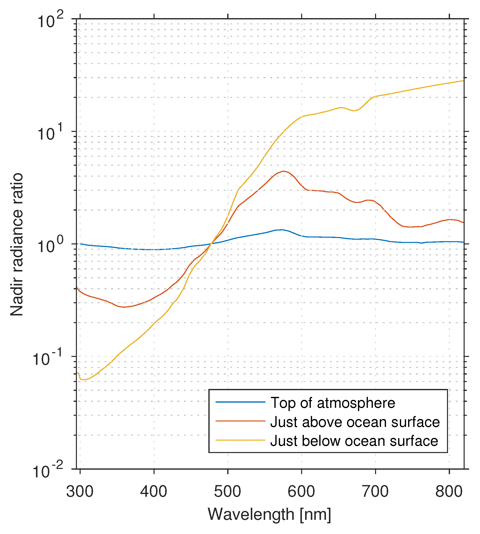
• there is a significant change in sub-surface color with increasing chlorophyll concentration, while at the same time
• there is only a slight change in color at the TOA, where the spectra are dominated by light from atmospheric scattering.

Most ocean color algorithms consist of two steps:

• First, one does an “atmospheric correction” (assuming the water to be black at NIR wavelengths) to determined the water-leaving radiance.
• Second, one retrieves the desired aquatic parameters from the water-leaving radiance.

In the visible, up to 90% of the radiance measured by a satellite sensor typically comes from the atmosphere implying that:

• Atmospheric correction becomes a very challenging task unless the near-infrared (NIR) black-pixel approximation (BPA) is valid.
• Estimation of diffuse transmittance is also important, but difficult because it depends on the angular distribution of the radiance just beneath the water surface.

Also, accurate characterization of the atmosphere is important because:

• a small uncertainty in the atmospheric correction may lead to a big error in the inferred aquatic parameters, and
• aerosol optical properties vary considerably in space and time.

5.4.1. The OC-SMART Optimal Estimation Approach

To address this situation, the OC-SMART (Ocean Color—Simultaneous Marine and Aerosol Retrieval Tool) approach was developed. The goal was to improve retrieval accuracy by use of AccuRT forward modeling and Optimal Estimation/Levenberg-Marquardt (OE/LM) inversion [108]:

• AccuRT: accurate discrete-ordinates radiative transfer model for the coupled atmosphere-ocean system; delivers a complete set of simulated radiances and Jacobians (weighting functions).
• OE/LM inversion: is an iterative, nonlinear least squares cost function minimization with a priori and Levenberg-Marquardt regularization.
• For retrievals of aerosol and aquatic parameters from Ocean Color data, we define a 5-element state vector:

  $$\mathbf{x}=\{{\tau }_{865},f_a,\mathbf{CHL},\mathbf{CDM},\mathbf{BBP}\}$$

  consisting of

  -

  2 aerosol parameters (${\tau }_{865}=$ optical depth at 865 nm and $f_a=$ bimodal fraction of particles),

  -

  3 marine parameters (chlorophyll concentration, CHL, combined absorption by detrital and dissolved material at 443 nm, CDM, and backscattering coefficient at 443 nm, BBP).

At each iteration step, the next estimate of the state vector is given by the OE/LM inversion [70]

$${\mathbf{x}}_{n+1}={\mathbf{x}}_n+{[(1+{\gamma }_n){\mathbf{S}}_a^{-1}+{\mathbf{J}}_n^T{\mathbf{S}}_m^{-1}{\mathbf{J}}_n]}^{-1}\{{\mathbf{J}}_n^T{\mathbf{S}}_m^{-1}({\mathbf{y}}_{\mathbf{m}}-{\mathbf{y}}_n)-({\mathbf{x}}_n-{\mathbf{x}}_a)\}.$$

(155)

In Equation (155) ${\mathbf{y}}_m$ is the vector of measured TOA radiances; ${\mathbf{y}}_n=\mathrm{F}({\mathbf{x}}_n,\mathit{b})$ is the vector of simulated TOA radiances generated by the AccuRT forward model; ${\mathbf{y}}_n$ is a (non-linear) function of the state vector ${\mathbf{x}}_n$ of retrieval elements, and $\mathit{b}$ represents model parameters; ${\mathbf{J}}_n$ is a matrix of simulated radiance partial derivatives with respect to the state vector elements ${\mathbf{x}}_n$ (the Jacobians); ${\mathbf{x}}_a$ and ${\mathbf{S}}_a$ are the a priori state vector and covariance matrix, respectively, and ${\mathbf{S}}_m$ is the measurement error covariance matrix. ${\gamma }_n$ is the Levenberg-Marquardt (LM) regularization parameter, When ${\gamma }_n\to 0$ Equation (155) becomes the standard Gauss-Newton Optimal Estimation (OE), and when ${\gamma }_n\to \infty$ it tends to the steepest descent method. AccuRT returns simulated radiances (${\mathbf{y}}_n$) and Jacobians (${\mathbf{J}}_n$) required to update the state vector estimate (${\mathbf{x}}_n$) according to Equation (155) above.

One issue with the OC-SMART approach is that it is relatively slow due to the need to call the forward AccuRT model repeatedly in the iterative inversion to compute radiances and Jacobians. To deal with that problem, one could use AccuRT instead to create a training ensemble in order to construct a Radial Basis Function Neural Network. This approach typically leads to an increase in computational speed by a factor of about 1000. In this way one replaces the AccuRT forward model (thousands of lines of code) with the following single equation (similar to Equation (151)):

$$I_i=\sum _{j=1}^N{a}_{ij}\exp [-b\sum _{k=1}^K{(P_k-c_{jk})}^2]+d_i$$

where $I_i$ it the TOA radiance in channel $i=1,\dots ,8$, $K=$ # of input parameters, and $a_{i,j},b,c_{j,k},d_i$ are the coefficients to be optimized in the network training.

The Jacobians (partial derivatives) $\mathbf{J}$ are also required for the non-linear optimal estimation using Equation (155). These Jacobians can be calculated by taking partial derivatives of $I_i$ respect to each input parameter:

$$J_{ik}=\frac{\partial I_i}{\partial P_k}=-2\sum _{j=1}^N{a}_{ij}{b}^2(P_k-c_{jk})\exp \{\sum _{k=1}^K{(P_k-c_{jk})}^2\}.$$

(156)

Fan et al. [107] applied the OC-SMART algorithm to a MODIS image obtained on 18 April 2014 over a Norwegian coastal area and compared retrieval results with the standard SeaDAS retrievals as shown in Figure 7 with OC-SMART results at the top and SeaDAS results at the bottom. From left to right, the columns are ${\tau }_{869}$, $f_a$, CHL, CDOM and $b_{bp}$, respectively. The first two columns are retrieved aerosol parameters. Our results are very similar to the SeaDAS retrievals, which makes sense because the two algorithms share the same aerosol model. However, the marine parameters show some differences and we should point out that in OC-SMART, we used the GSM bio-optical model when we retrieved the ocean parameters. The SeaDAS CHL retrieval shown in Figure 7 is from the OC4v6 algorithm. SeaDAS failed when using the GSM model due to negative water-leaving radiances resulting from an incorrect atmospheric correction, which is a common issue in traditional atmospheric correction algorithms. The aerosol optical depths was determined at a near infrared (NIR) wavelength (${\tau }_{869}$) and then extrapolated to shorter wavelengths. Since the water-leaving radiance is only a small fraction of the TOA radiance measured by the satellite instrument, a small error in the aerosol retrieval may cause the water-leaving radiance to become negative. We also found the OC-SMART results to be close to the field measurements. The CHL value was 0.56 [$\mathrm{mg}/{\mathrm{m}}^3$] while the field measurements showed an average of 0.86 ± 0.34 [$\mathrm{mg}/{\mathrm{m}}^3$] in the spring season. The CDOM absorption coefficient was 0.15 [${\mathrm{m}}^{-1}$] and the field measurements show an average of 0.14 ± 0.06 [${\mathrm{m}}^{-1}$].

5.4.2. The OC-SMART Multilayer Neural Network Approach

In open ocean areas where the water IOPs are correlated with pigmented particles, standard atmospheric correction (AC) algorithms seem to work reasonably well. However, in turbid coastal water areas the IOPs of suspended inorganic particles, and colored dissolved organic matter (CDOM) may vary independently of pigmented particles. Therefore, in turbid coastal waters standard AC algorithms often exhibit large inaccuracies that may lead to highly uncertain and frequently negative water-leaving radiances ($L_{\mathrm{w}}$) or remote sensing reflectances ($R_{\mathrm{rs}}$ values). To address this problem, Fan et al. [109] introduced a new atmospheric correction algorithm for coastal water areas based on a multilayer neural network (MLNN) method. A coupled atmosphere-ocean radiative transfer model (AccuRT) was used to simulate the Rayleigh-corrected radiance ($L_{\mathrm{rc}}$) at the TOA and the $R_{\mathrm{rs}}$ just above the surface simultaneously, and to train a MLNN to derive the aerosol optical depth (AOD) and $R_{\mathrm{rs}}$ values directly from the TOA $L_{\mathrm{rc}}$. The method was validated using both a synthetic dataset and Aerosol Robotic Network–Ocean Color (AERONET–OC) measurements.

Extensive testing has shown that this MLNN approach has several advantages [109]:

• It significantly improved the quality of retrieved remote sensing reflectances (compared to the SeaDAS NIR algorithm) by reducing the average percentage difference (APD) between MODIS retrievals and ground-truth (AERONET-OC) validation data.
• In highly absorbing coastal water, such as the Baltic Sea, it provides reduction of the APD by more than 60%, and in highly scattering water, such as the Black Sea, it provides reduction of the APD by more than 25%.
• It is robust and resilient to contamination due to sunglint and adjacency effects of land and cloud edges.
• It is applicable in extreme conditions such as those encountered for heavily polluted continental aerosols, extreme turbid water, and dust storms.
• It does not require shortwave infrared (SWIR) bands, and is therefore suitable for all ocean color sensors.
• It is very fast and suitable for operational use.

Recent addition of training data to make it representative for a variety of water types has shown that this approach can produce a seamless (smooth) transition between turbid coastal water areas and clean open ocean areas.

5.4.3. Issues Specific to Geostationary Platforms

Low Solar Elevations 

With geostationary platforms one has the opportunity to investigate diurnal variations in water properties. Hence, there is a desire to obtain useful observations throughout the day from sunrise to sunset. However, for solar zenith angles larger than about 75${}^{\circ }$ (and large viewing angles) the plane-parallel approximation (PPA) becomes invalid, and we need to take Earth curvature into account, as discussed in a recent paper [110]. An approximate way to deal with this problem is the so-called pseudo-spherical approximation (PSA), in which the direct beam single scattering (solar pseudo-source) term is treated in spherical geometry: $e^{-\tau /{\mu }_0}\to e^{-\tau Ch\left({\mu }_0\right)}$, where the Chapman function $Ch\left({\mu }_0\right)$ takes curvature into account [14,110], while the multiple scattering term is treated using the PPA. Hence, in the PSA the RTE becomes:

$$\begin{array}{ccc}\hfill u\frac{dI(\tau ,u,\varphi )}{d\tau }& =& I(\tau ,u,\varphi )-\stackrel{\mathrm{multiple}\mathrm{scattering}}{\overbrace{\frac{\varpi \left(\tau \right)}{4\pi }{\int }_0^{2\pi }d{\varphi }^{\prime }{\int }_{-1}^{1}d{u}^{\prime }p(\tau ,u^{\prime },{\varphi }^{\prime };u,\varphi )I(\tau ,u^{\prime },{\varphi }^{\prime })}}\hfill \\ & & -\stackrel{\mathrm{single}\mathrm{scattering}}{\overbrace{\frac{\varpi \left(\tau \right)}{4\pi }p(\tau ,-{\mu }_0,{\varphi }_0;u,\varphi )F_0{e}^{-\tau Ch\left({\mu }_0\right)}}}.\hfill \end{array}$$

(157)

It should be pointed out that low solar elevations is generally a problem at high latitudes also for polar-orbiting platforms.

Surface Roughness Considerations 

As alluded to above, it would be worthwhile considering the advantage gained by using a 2D rather than a 1D slope distribution to deal with a wind-roughened surface (see Figure 4). Hence, one should consider using

• a 2D Gaussian surface slope distribution for singly scattered light, and
• a 1D Gaussian surface slope distribution for multiply scattered light.

Such an approach may be quite successful, as demonstrated in Figure 3, because a 2D BRDF simulates sunglint very well, while a 1D BRDF is sufficient to simulate the smoother (more directionally uniform) skylight.

Use of Vector (Polarized) RT Simulations 

Analysis of polarization measurements require vector RT modeling [111], and retrieval results from radiance-only measurements are likely to be improved by employing a vector (polarized) forward RT model to compute the radiances and Jacobians used in the inversion step, particularly for modeling the radiance due to scattering by small aerosol particles at short wavelengths. Also, the increased information from polarization measurements can lead to significant improvements in atmospheric correction due to aerosols [112]. Hence, for ocean color retrievals from geostationary platforms, we should explore the advantage of using the pseudo-spherical approximation combined with

• polarized (vector) radiative transfer simulations,
• a 2D Gaussian distribution of surface slopes,

and neural networks and optimal estimation for

• simultaneous retrieval of atmospheric and marine parameters from multi-spectral as well as hyperspectral measurements of total and polarized (if available) radiances, and
• assessments of retrieval accuracy and error budgets.

6. Remaining Problems

6.1. 3-D Radiative Transfer: The LiDAR Problem

Although we have mostly considered plane-parallel systems so far with an emphasis on the coupling between the atmosphere and the underlying surface consisting of a water body or a snow/ice surface, there are many applications that require a three-dimensional (3-D) RT treatment. For a clear (cloud- and aerosol-free) atmosphere, 3-D effects are related to the impact of the Earth’s curvature on the radiation field as discussed briefly in Section 5.4.3. To include Earth curvature effects it may be sufficient to employ a “pseudo-spherical” treatment, in which the direct solar beam illumination is treated in spherical geometry [110,113], whereas multiple scattering is treated in plane-parallel geometry. In fact, this pseudo-spherical approach has been implemented in many RT codes [114,115]. Also, there is a large body of literature on 3-D RT modeling with applications to broken clouds, and readers interested in this topic may want to consult [116] or visit the web-site http://i3rc.gsfc.nasa.gov/.

Finally, 3-D RT modeling may also be important for analysis and interpretation of LiDAR data. The classical “searchlight problem” [117], which considers the propagation of a laser beam through a turbid medium, is relevant in this context. Long-range propagation of a LiDAR beam has been studied both theoretically and experimentally [118]. Monte Carlo simulations are well suited for such studies [119], and use of deterministic models such the discrete-ordinate method, briefly discussed in Section 4, have also been pursued to investigate this problem [120,121].

6.2. Time-Dependent Radiative Transfer

Most studies of radiative transfer in the ocean have been concerned with understanding the propagation of sunlight through natural water bodies [3,4,14,122]. For such applications, the transient or time-dependent term in the RTE can be ignored, because changes in the incident illumination are much slower than the changes imposed by light propagation through the coupled atmosphere-water system. While this assumption is satisfied for solar illumination, LiDAR systems can use pulses that are shorter than the attenuation distance of seawater divided by the speed of light in water. Also, it has been pointed out [123] that due to multiple light scattering, understanding the LiDAR signal requires a solution of the time-dependent RTE. The transient RT problem can be reduced to solving a series of time-independent RT problems [124].

6.3. Other Issues

Although inelastic scattering processes (Raman and Brillouin) certainly can be very important and indeed essential in some atmospheric [125,126,127] and aquatic [128,129] applications, we have limited our discussion to elastic scattering. In fact, inelastic scattering effects can become important for very clear water and sky conditions.

Forward radiative transfer models need accurate IOPs as input. Therefore, in situ measurements are needed of the scattering phase function of hydrosols in clear as well as turbid (coastal) water, including measurements at a scattering angle close to 180${}^{\circ }$. The 180${}^{\circ }$-backscatter angle is of particular interest for LiDAR applications. In view of the growing interest in applications based on RT models for coupled systems [84,86,87,90,91,92,93], there is also a need for systematic and sustained measurements of the scattering phase (or Muller) matrix, since not much work has been done after the 1984 Voss and Fry publication [130].

To process hyperspectral data one needs algorithms that can handle large data volumes and deal with measurement uncertainties in a proper manner. In general, better bio-optical models are also needed. For example, the approximation that the spectral slope $\nu =0$ for CHL > 2.0 in Equation (97) is problematic. Hyperspectral (and potentially polarimetric) measurements are needed to construct more generally applicable bio-optical models.

In Section 5.4.2 we discussed how a forward-inverse modeling approach, based on AccuRT simulations for the coupled atmosphere-water system combined with a multilayer neural network (MLNN), can be used to infer accurate remote sensing reflectances ($R_{\mathrm{rs}}$ values) from clear as well as turbid water [109]. The logical next step is to use these $R_{\mathrm{rs}}$ values to infer water IOPs. In fact, several semi-analytic algorithms have been developed for this purpose including the generalized IOP (GIOP) algorithm described by Werdell and colleagues [131].

This GIOP approach is currently the default algorithm used by NASA for processing of MODIS ocean color data. First, the $R_{\mathrm{rs}}$ values are obtained after an atmospheric correction step using NIR channels. Ocean IOP parameters are then retrieved from the approximate $R_{\mathrm{rs}}$ values (based on many assumptions) by performing a non-linear inversion. The QAA algorithm [132] is another semi(quasi)-analytic algorithm, similar to the GIOP, that performs better than the GIOP in some situations. The GIOP and QAA algorithms generally perform well over the open ocean, but can have significant issues in coastal water because the atmospheric correction method produces inaccurate $R_{\mathrm{rs}}$ values that lead to large errors in derived IOPs. Furthermore, the performance of the atmospheric correction is worse the farther the extrapolation is taken from the NIR to shorter wavelengths, which is a problem for ocean color sensors with UV channels. Also, particle size distribution and scattering phase function constitute a priori information in the semi-analytic algorithms that cannot be retrieved. These limitations make them unsuitable for application to new sensors with increased information content, such as hyperspectral ocean color sensors. Instruments that can measure the polarization of light will also be extremely useful for improving aerosol retrievals and thus atmospheric correction capabilities. The next generation of sensors composed of hyperspectral polarimeters and ocean-capable LiDAR instruments will enable the use of more advanced retrieval algorithms to more accurately quantify and monitor the atmosphere-ocean system, particularly in coastal areas. Nevertheless, use of accurate $R_{\mathrm{rs}}$ values, obtained from new and improved AC methods, such as the MLNN algorithm [109], in existing semi-analytic algorithms (like GIOP and QAA) is expected to significantly enhance their performance when applied to current ocean color sensor data obtained over turbid water.

7. Summary

A review has been provided of forward and inverse radiative transfer modeling in coupled systems consisting of two adjacent, horizontal slabs with different indices of refraction and a rough interface characterized by a Gaussian distribution of surface slopes in one or two dimensions. Such a configuration can be used to simulate radiative transfer in coupled atmosphere-snow/ice-ocean systems. Input and output parameters including boundary conditions for the forward radiative transfer problem were introduced in Section 2, while in Section 3 a review was provided of inherent optical properties (IOPs) of the atmosphere, snow/ice and ocean water. These IOPs are required inputs to the radiative transfer equation introduced in Section 4 both for unpolarized (scalar) and polarized (vector) radiative transfer. Examples of how to solve inverse problems occurring in remote sensing of the environment employing optimization techniques as well as the unique power of machine learning (neural networks) for convenience and efficiency were provided in Section 5. Finally, in Section 6 some remaining radiative transfer problems were discussed.

References

1. Ricchiazzi, P.; Yang, S.; Gautier, C.; Sowle, D. SBDART: A research and teaching software tool for plane-parallel radiative transfer in the Earth’s atmosphere. Bull. Am. Meteorol. Soc. 1998, 79, 2101–2114. [Google Scholar] [CrossRef]
2. Key, J.R.; Schweiger, A.J. Tools for atmospheric radiative transfer: Streamer and FluxNet. Comput. Geosci. 1998, 24, 443–451. [Google Scholar] [CrossRef] [Green Version]
3. Stamnes, K.; Stamnes, J.J. Radiative Transfer in Coupled Environmental Systems; Wiley-VCH: Weinheim, Germany, 2015. [Google Scholar]
4. Mobley, C.D. Light and Water; Academic Press: Cambridge, MA, USA, 1994. [Google Scholar]
5. Hovenier, J.W.; der Mee, C.D.V.; Domke, H. Transfer of Polarized Light in Planetary Atmospheres; Kluwer Academic Publsihers: Dordrecht, The Netherlands, 2004. [Google Scholar]
6. Rayleigh, L. A re-examination of the light scattered by gases in respect of polarization. II. Experiments on helium and argon. Proc. R. Soc. 1920, 98, 57–64. [Google Scholar] [CrossRef]
7. Morel, A. Optical properties of pure water and pure seawater. In Optical Aspects of Oceanography; Jerlov, N.G., Nielsen, E.S., Eds.; Academic Press: Cambridge, MA, USA, 1974; pp. 1–24. [Google Scholar]
8. Morel, A.; Gentili, B. Diffuse reflectance of oceanic waters: its dependence on sun angle as influenced by the molecular scattering contribution. Appl. Opt. 1991, 30, 4427–4437. [Google Scholar] [CrossRef] [PubMed]
9. Rayleigh, L. On the light from the sky, its polarization and colour. Philos. Mag. 1871, 41, 107–120, 274–279, 447–454. [Google Scholar]
10. Bodhaine, B.; Wood, N.; Dutton, E.; Slusser, J. On Rayleigh optical depth calculations. J. Atmos. Ocean. Technol. 1999, 16, 1854–1861. [Google Scholar] [CrossRef]
11. Farinato, R.S.; Rowell, R.L. New values of the light scattering depolarization and anisotropy of water. J. Chem. Phys. 1976, 65, 593–595. [Google Scholar] [CrossRef]
12. Zhang, X.; Hu, L. Estimating scattering of pure water from density fluctuation of the refractive index. Opt. Express 2009, 17, 1671–1678. [Google Scholar] [CrossRef] [PubMed]
13. Henyey, L.C.; Greenstein, J.L. Diffuse radiation in the galaxy. Astrophys. J. 1941, 93, 70–83. [Google Scholar] [CrossRef]
14. Stamnes, K.; Thomas, G.E.; Stamnes, J.J. Radiative Transfer in the Atmosphere and Ocean, 2nd ed.; Cambridge University Press: Cambridge, UK, 2017. [Google Scholar]
15. Hovenier, J.W.; van der Mee, C.V.M. Fundamental relationships relevant to the transfer of polarized light in a scattering atmosphere. Astron. Astrophys. 1983, 128, 1–16. [Google Scholar]
16. Chandrasekhar, S. Radiative Transfer; Dover Publications: Mineola, NY, USA, 1960. [Google Scholar]
17. De Haan, J.; Bosma, P.; Hovenier, J. The adding method for multiple scattering calculations of polarized light. Astron. Astrophys. 1987, 183, 371–391. [Google Scholar]
18. Siewert, C. A discrete-ordinates solution for radiative-transfer models that include polarization effects. J. Quant. Spectrosc. Radiat. Transf. 2000, 64, 227–254. [Google Scholar] [CrossRef] [Green Version]
19. Cohen, D.; Stamnes, S.; Tanikawa, T.; Sommersten, E.R.; Stamnes, J.J.; Lotsberg, J.K.; Stamnes, K. Comparison of Discrete Ordinate and Monte Carlo Simulations of Polarized Radiative Transfer in two Coupled Slabs with Different Refractive Indices. Opt. Express 2013, 21, 9592–9614. [Google Scholar] [CrossRef] [PubMed]
20. Siewert, C.E. On the equation of transfer relevant to the scattering of polarized light. Astrophys. J. 1981, 245, 1080–1086. [Google Scholar] [CrossRef]
21. Siewert, C.E. On the phase matrix basic to the scattering of polarized light. Astron. Astrophys. 1982, 109, 195–200. [Google Scholar]
22. Sommersten, E.R.; Lotsberg, J.K.; Stamnes, K.; Stamnes, J.J. Discrete ordinate and Monte Carlo simulations for polarized radiative transfer in a coupled system consisting of two media with different refractive indices. J. Quant. Spectrosc. Radiat. Transf. 2010, 111, 616–633. [Google Scholar] [CrossRef]
23. Mishchenko, M.I. Light scattering by randomly oriented rotationally symmetric particles. J. Opt. Soc. Am. A 1991, 8, 871–882. [Google Scholar] [CrossRef]
24. Mishchenko, M.I.; Travis, L.D. Satellite retrieval of aerosol properties over the ocean using polarization as well as intensity of reflected sunlight. J. Geophys. Res. 1997, 102, 16989–17013. [Google Scholar] [CrossRef] [Green Version]
25. Anderson, G.P.; Clough, S.A.; Kneizys, F.X.; Chetwynd, J.H.; Shettle, E.P. AFGL Atmospheric Constituent Profiles (0–120 km), AFGL-TR-86-0110 (OPI); Optical Physics Division, Air Force Geophysics Laboratory Hanscom AFB: Bedford, MA, USA, 1986. [Google Scholar]
26. Berk, A.; Anderson, G.P.; Acharya, P.K.; Bernstein, L.S.; Muratov, L.; Lee, J.; Fox, M.; Adler-Golden, S.M.; Chetwynd, J.H.; Hoke, M.L.; et al. MODTRAN 5: A Reformulated Atmospheric Band Model with Auxiliary Species and Practical Multiple Scattering Options: Update; Defense and Security, International Society for Optics and Photonics: Orlando, FL, USA, 2005; pp. 662–667. [Google Scholar]
27. Berk, A.; Conforti, P.; Kennett, R.; Perkins, T.; Hawes, F.; van den Bosch, J. MODTRAN6: A Major Upgrade of the MODTRAN Radiative Transfer Code; SPIE Defense+ Security, International Society for Optics and Photonics: Orlando, FL, USA, 2014; p. 90880H. [Google Scholar]
28. Kneizys, F.X.; Abreu, L.W.; Anderson, G.; Chetwynd, J.; Shettle, E.; Berk, A.; Bernstein, L.; Roberson, D.; Acharya, P.; Rothman, L.; et al. MODTRAN2/3 Report and LOWTRAN 7 Model; Technical Report; Phillips Laboratory, Hanscom AFB: Bedford, MA, USA, 1996. [Google Scholar]
29. Chen, N.; Li, W.; Tanikawa, T.; Hori, M.; Shimada, R.; Aoki, T.; Stamnes, K. Fast yet accurate computation of radiances in shortwave infrared satellite remote sensing channels. Opt. Express 2017, 25, A649–A664. [Google Scholar] [CrossRef] [PubMed]
30. Ahmad, Z.; Franz, B.A.; McClain, C.R.; Kwiatkowska, E.J.; Werdell, J.; Shettle, E.P.; Holben, B.N. New aerosol models for the retrieval of aerosol optical thickness and normalized water-leaving radiances from the SeaWiFS and MODIS sensors over coastal regions and open oceans. Appl. Opt. 2010, 49, 5545–5560. [Google Scholar] [CrossRef] [PubMed]
31. Hess, M.; Koepke, P.; Schult, I. Optical properties of aerosols and clouds: The software package OPAC. Bull. Am. Met. Soc. 1998, 79, 831–844. [Google Scholar] [CrossRef]
32. Davies, C.N. Size distribution of atmospheric particles. J. Aerosol Sci. 1974, 5, 293–300. [Google Scholar] [CrossRef]
33. Holben, B.N.; Eck, T.F.; Slutsker, I.; Tanre, D.; Buis, J.P.; Setzer, A.; Vermote, E.; Reagan, J.A.; Kaufman, Y.; Nakajima, T.; et al. AERONET—A federated instrument network and data archive for aerosol characterization. Remote Sens. Environ. 1998, 66, 1–16. [Google Scholar] [CrossRef]
34. Holben, B.N.; Tanre, D.; Smirnov, A.; Eck, T.F.; Slutsker, I.; Abuhassan, N.; Newcomb, W.W.; Schafer, J.; Chatenet, B.; Lavenue, F.; et al. An emerging ground-based aerosol climatology: aerosol optical depth from AERONET. J. Geophys. Res. 2001, 106, 12067–12097. [Google Scholar] [CrossRef]
35. Hansen, J.E.; Travis, L.D. Light scattering in planetary atmospheres. Space Sci. Rev. 1974, 16, 527–610. [Google Scholar] [CrossRef]
36. Hänel, G. The properties of atmospheric aerosol particles as functions of the relative humidity at thermodynamic equilibrium with the surrounding moist air. In Advances in Geophysics; Landsberg, H.E., Miehem, J.V., Eds.; Elsevier: New York, NY, USA, 1976; Volume 19. [Google Scholar]
37. Shettle, E.P.; Fenn, R.W. Models for the Aerosols of the Lower Atmosphere and the Effects of Humidity Variations on their Optical Properties; Air Force Geophysics Laboratory, Hanscomb AFB: Bedford, MA, USA, 1979. [Google Scholar]
38. Yan, B.; Stamnes, K.; Li, W.; Chen, B.; Stamnes, J.J.; Tsay, S.C. Pitfalls in atmospheric correction of ocean color imagery: How should aerosol optical properties be computed? Appl. Opt. 2002, 41, 412–423. [Google Scholar] [CrossRef] [PubMed]
39. Du, H. Mie-scattering calculation. Appl. Opt. 2004, 43, 1951–1956. [Google Scholar] [CrossRef] [PubMed]
40. Wendisch, M.; Yang, P. Theory of Atmospheric Radiative Transfer; John Wiley & Sons: Hoboken, NJ, USA, 2012. [Google Scholar]
41. Segelstein, D.J. The Complex Refractive Index of Water. Mater’s Thesis, Department of Physics, University of Missouri, Kansas City, MO, USA, 1981. [Google Scholar]
42. Smith, R.C.; Baker, K.S. Optical properties of the clearest natural waters (200–800 nm). Appl. Opt. 1981, 36, 177–184. [Google Scholar] [CrossRef] [PubMed]
43. Sogandares, F.M.; Fry, E.S. Absorption spectrum (340–640 nm) off pure water. I. Photothermal measurements. Appl. Opt. 1997, 36, 8699–8709. [Google Scholar] [CrossRef] [PubMed]
44. Pope, R.M.; Fry, E.S. Absorption spectrum (380–700 nm) of pure water, II Integrating cavity measurements. Appl. Opt. 1997, 36, 8710–8723. [Google Scholar] [CrossRef] [PubMed]
45. Kou, L.; Labrie, D.; Chylek, P. Refractive indices of water and ice in the 0.65 μm to 2.5 μm spectral range. Appl. Opt. 1993, 32, 3531–3540. [Google Scholar] [CrossRef] [PubMed]
46. Wiscombe, W.J.; Warren, S.G. A Model for the Spectral Albedo of Snow. I: Pure Snow. J. Atmos. Sci. 1980, 37, 2712–2733. [Google Scholar] [CrossRef] [Green Version]
47. Warren, S.G.; Wiscombe, W.J. A Model for the Spectral Albedo of Snow. II: Snow Containing Atmospheric Aerosols. J. Atmos. Sci. 1980, 37, 2734–2745. [Google Scholar] [CrossRef] [Green Version]
48. Grenfell, T.S.; Warren, S.G.; Mullen, P.C. Reflection of solar radiation by the Antarctic snow surface at ultraviolet, visible, and near?infrared wavelengths. J. Geophys. Res. 1994, 99, 18669–18684. [Google Scholar] [CrossRef]
49. Warren, S.G.; Brandt, R.E. Optical constants of ice from the ultraviolet to the microwave: A revised compilation. J. Geophys. Res. Atmos. 2008, 113. [Google Scholar] [CrossRef] [Green Version]
50. Jin, Z.; Stamnes, K.; Weeks, W.F.; Tsay, S.C. The effect of sea ice on the solar energy budget in the atmosphere-sea ice-ocean system: A model study. J. Geophys. Res. 1994, 99, 25281–25294. [Google Scholar] [CrossRef]
51. Hamre, B.; Winther, J.G.; Gerland, S.; Stamnes, J.J.; Stamnes, K. Modeled and measured optical transmittance of snow-covered first-year sea ice in Kongsfjorden, Svalbard. J. Geophys. Res. Oceans 2004, 109. [Google Scholar] [CrossRef] [Green Version]
52. Jiang, S.; Stamnes, K.; Li, W.; Hamre, B. Enhanced solar irradiance across the atmosphere–sea ice interface: A quantitative numerical study. Appl. Opt. 2005, 44, 2613–2625. [Google Scholar] [CrossRef] [PubMed]
53. Stamnes, K.; Hamre, B.; Stamnes, J.J.; Ryzhikov, G.; Birylina, M.; Mahoney, R.; Hauss, B.; Sei, A. Modeling of radiation transport in coupled atmosphere-snow-ice-ocean systems. J. Quant. Spectrosc. Radiat. Transf. 2011, 112, 714–726. [Google Scholar] [CrossRef]
54. Ackermann, M.; Ahrens, J.; Bai, X.; Bartelt, M.; Barwick, S.W.; Bay, R.C.; Becka, T.; Becker, J.K.; Becker, K.H.; Berghaus, P.; et al. Optical properties of deep glacial ice at the South Pole. J. Geophys. Res. 2006, 111. [Google Scholar] [CrossRef] [Green Version]
55. Fialho, P.; Hansen, A.D.A.; Honrath, R.E. Absorption coefficients by aerosols in remote areas: A new approach to decouple dust and black carbon absorption coefficients using seven-wavelength Aethalometer data. J. Aerosol Sci. 2005, 36, 267–282. [Google Scholar] [CrossRef]
56. Twardowski, M.S.; Boss, E.; Sullivan, J.M.; Donaghay, P.L. Modeling the spectral shape of absorption by chromophoric dissolved organic matter. Mar. Chem. 2004, 89, 69–88. [Google Scholar] [CrossRef]
57. Uusikivi, J.; Vähätalo, A.V.; Granskog, M.A.; Sommaruga, R. Contribution of mycosporine-like amino acids and colored dissolved and particulate matter to sea ice optical properties and ultraviolet attenuation. Limnol. Oceanogr. 2010, 55, 703–713. [Google Scholar] [CrossRef] [PubMed] [Green Version]
58. Ruddick, K.; Bouchra, N.; Collaborators. Coastcoulor Round Robin—Final Report. 2013. Available online: ftp://[email protected]/RoundRobin/CCRR_report_OCSMART.pdf (accessed on 12 April 2018).
59. Babin, M.; Stramski, A.D.; Ferrari, G.M.; Claustre, H.; Bricaud, A.; Obelesky, G.; Hoepffner, N. Variations in the light absorption coefficients of phytoplankton, nonalgal particles and dissolved organic matter in coastal waters around Europe. J. Geophys. Res. 2003, 108. [Google Scholar] [CrossRef]
60. Babin, M.; Morel, A.; Fournier-Sicre, V.; Fell, F.; Stramski, D. Light scattering properties of marine particles in coastal and open ocean waters as related to the particle mass concentration. Limnol. Oceanogr. 2003, 28, 843–859. [Google Scholar] [CrossRef]
61. Bricaud, A.; Morel, A.; Babin, M.; Allali, K.; Claustre, H. Mie-Scattering Calculation. J. Geophys. Res. 1998, 103, 31033–31044. [Google Scholar] [CrossRef]
62. Loisel, H.; Morel, A. Light scattering and chlorophyll concentration in case 1 waters: A re-examination. Limnol. Oceanogr. 1998, 43, 847–857. [Google Scholar] [CrossRef]
63. Morel, A.; Antoine, D.; Gentili, B. Bidirectional reflectance of oceanic waters: Accounting for Raman emission and varying particle scattering phase function. Appl. Opt. 2002, 41, 6289–6306. [Google Scholar] [CrossRef] [PubMed]
64. Mobley, C.P.; Sundman, L.K.; Boss, E. Phase function effects on oceanic light fields. Appl. Opt. 2002, 41, 1035–1050. [Google Scholar] [CrossRef] [PubMed]
65. Diehl, P.; Haardt, H. Measurement of the spectral attenuation to support biological research in a “plankton tube” experiment. Oceanol. Acta 1980, 3, 89–96. [Google Scholar]
66. McCave, I.N. Particulate size spectra, behavior, and origin of nephloid layers over the Nova Scotia continental rise. J. Geophys. Res. 1983, 88, 7647–7660. [Google Scholar] [CrossRef]
67. Fournier, G.R.; Forand, J.L. Analytic phase function for ocean water. Proc. SPIE Ocean Opt. XII 1994, 2558, 194–202. [Google Scholar]
68. Hu, Y.X.; Wielicki, B.; Lin, B.; Gibson, G.; Tsay, S.C.; Stamnes, K.; Wong, T. Delta-fit: A fast and accurate treatment of particle scattering phase functions with weighted singular-value decomposition least squares fitting. J. Quant. Spectrosc. Radiat. Transf. 2000, 65, 681–690. [Google Scholar] [CrossRef]
69. Werdell, P.; Bailey, S. An improved in-situ bio-optical data set for ocean color algorithm development and satellite data product validation. Remote Sens. Environ. 2005, 98, 122–140. [Google Scholar] [CrossRef]
70. Li, W.; Stamnes, K.; Spurr, R.; Stamnes, J.J. Simultaneous Retrieval of Aerosols and Ocean Properties: A Classic Inverse Modeling Approach. II. SeaWiFS Case Study for the Santa Barbara Channel. Int. J. Rem. Sens. 2008, 29, 5689–5698. [Google Scholar] [CrossRef]
71. Garver, S.A.; Siegel, D. Inherent optical property inversion of ocean color spectra and its biogeochemical interpretation 1. Time series from the Sargasso Sea. J. Geophys. Res. 1997, 102, 18607–18625. [Google Scholar] [CrossRef]
72. Garver, S.A.; Siegel, D.; Peterson, A.R. Optimization of a semi-analytical ocean color model for global-scale applications. Appl. Opt. 2002, 41, 2705–2714. [Google Scholar]
73. Bohren, C.F.; Huffman, D.R. Absorption and Scattering of Light by Small Particles; John Wiley: New York, NY, USA, 1998. [Google Scholar]
74. Born, M.; Wolf, E. Principles of Optics; Cambridge University Press: Cambridge, UK, 1980. [Google Scholar]
75. Cox, C.; Munk, W. Measurement of the roughness of the sea surface from photographs of the sun’s glitter. J. Opt. Soc. Am. 1954, 44, 838–850. [Google Scholar] [CrossRef]
76. Masuda, K. Effects of the speed and direction of surface winds on the radiation in the atmosphere—Ocean system. Remote Sens. Environ. 1998, 64, 53–63. [Google Scholar] [CrossRef]
77. Wang, M.; Bailey, S.W. Correction of sun glint contamination on the SeaWiFS ocean and atmosphere products. Appl. Opt. 2001, 40, 4790–4798. [Google Scholar] [CrossRef]
78. Nakajima, T.; Tanaka, M. Algorithms for radiative intensity calculations in moderately thick atmospheres using a truncation approximation. J. Quant. Spectrosc. Radiat. Transf. 1988, 40, 51–69. [Google Scholar] [CrossRef]
79. Lin, Z.; Stamnes, S.; Jin, Z.; Laszlo, I.; Tsay, S.C.; Wiscombe, W.; Stamnes, K. Improved discrete ordinate solutions in the presence of an anisotropically reflecting lower boundary: Upgrades of the DISORT computational tool. J. Quant. Spectrosc. Radiat. Transf. 2015, 157, 119–134. [Google Scholar] [CrossRef]
80. Lin, Z.; Li, W.; Gatebe, C.; Poudyal, R.; Stamnes, K. Radiative transfer simulations of the two-dimensional ocean glint reflectance and determination of the sea surface roughness. Appl. Opt. 2016, 55, 1206–1215. [Google Scholar] [CrossRef] [PubMed]
81. Gordon, H.R. Atmospheric correction of ocean color imagery in the Earth Observation System era. J. Geophys. Res. 1997, 102, 17081–17106. [Google Scholar] [CrossRef]
82. Rodgers, C.D. Inverse Methods for Atmospheric Sounding: Theory and Practice; World Scientific: London, UK, 2000. [Google Scholar]
83. Jin, Z.; Stamnes, K. Radiative transfer in nonuniformly refracting layered media: Atmosphere-ocean system. Appl. Opt. 1994, 33, 431–442. [Google Scholar] [CrossRef] [PubMed]
84. Zhai, P.W.; Hu, Y.; Chowdhary, J.; Trepte, C.R.; Lucker, P.L.; Josset, D.B. A vector radiative transfer model for coupled atmosphere and ocean systems with a rough interface. J. Quant. Spectrosc. Radiat. Transf. 2010, 111, 1025–1040. [Google Scholar] [CrossRef]
85. Chowdhary, J.; Cairns, B.; Travis, L.D. Case studies of aerosol retrievals over the ocean from multiangle, multispectral photopolarimetric remote sensing data. J. Atmos. Sci. 2002, 59, 383–397. [Google Scholar] [CrossRef]
86. Chowdhary, J.; Cairns, B.; Mishchenko, M.I.; Hobbs, P.V.; Cota, G.F.; Redemann, J.; Rutledge, K.; Holben, B.N.; Russell, E. Retrieval of aerosol scattering and absorption properties from photopolarimetric observations over the ocean during the CLAMS experiment. J. Atmos. Sci. 2005, 62, 1093–1117. [Google Scholar] [CrossRef]
87. Chowdhary, J.; Cairns, B.; Waquet, F.; Knobelspiesse, K.; Ottaviani, M.; Redemann, J.; Travis, L.; Mishchenko, M. Sensitivity of multiangle, multispectral polarimetric remote sensing over open oceans to water-leaving radiance: Analyses of RSP data acquired during the MILAGRO campaign. Remote Sens. Environ. 2012, 118, 284–308. [Google Scholar] [CrossRef]
88. Chami, M.; Santer, R.; Dilligeard, E. Radiative transfer model for the computation of radiance and polarization in an ocean–atmosphere system: Polarization properties of suspended matter for remote sensing. Appl. Opt. 2001, 40, 2398–2416. [Google Scholar] [CrossRef] [PubMed]
89. Min, Q.; Duan, M. A successive order of scattering model for solving vector radiative transfer in the atmosphere. J. Quant. Spectrosc. Radiat. Transf. 2004, 87, 243–259. [Google Scholar] [CrossRef]
90. Fischer, J.; Grassl, H. Radiative transfer in an atmosphere-ocean system: An azimuthally dependent matrix-operator approach. Appl. Opt. 1984, 23, 1032–1039. [Google Scholar] [CrossRef] [PubMed]
91. Ota, Y.; Higurashi, A.; Nakajima, T.; Yokota, T. Matrix formulations of radiative transfer including the polarization effect in a coupled atmosphere-ocean system. J. Quant. Spectrosc. Radiat. Transfer 2010, 111, 878–894. [Google Scholar] [CrossRef]
92. Kattawar, G.; Adams, C. Stokes vector calculations of the submarine light field in an atmosphere-ocean with scattering according to the Rayleigh phase matrix: Effect of interface refractive index on radiance and polarization. Limnol. Oceanogr. 1989, 34, 1453–1472. [Google Scholar] [CrossRef]
93. Lotsberg, J.; Stamnes, J. Impact of particulate oceanic composition on the radiance and polarization of underwater and backscattered light. Opt. Express 2010, 18, 10432–10445. [Google Scholar] [CrossRef] [PubMed]
94. Morel, A.; Gentili, B. Diffuse reflectance of oceanic waters. II. bidirectional aspect. Appl. Opt. 1993, 32, 2803–2804. [Google Scholar] [CrossRef] [PubMed]
95. Fan, Y.; Li, W.; Stamnes, K.; Gatebe, C. A neural network method to correct bidirectional effects in water-leaving radiance. Appl. Opt. 2016, 55, 10–421. [Google Scholar] [CrossRef] [PubMed]
96. Voss, K.J.; Chapin, A.L. An Upwelling Radiance Distribution Camera System, NURADS. Opt. Express 2005, 13, 4250–4262. [Google Scholar] [CrossRef] [PubMed]
97. Kay, S.; Hedley, J.D.; Lavender, S. Sun Glint Correction of High and Low Spatial Resolution Images of Aquatic Scenes: A Review of Methods for Visible and Near-Infrared Wavelengths. Remote Sens. 2009, 1, 697–730. [Google Scholar] [CrossRef]
98. Steinmetz, F.; Deschamps, P.Y.; Ramon, D. Atmospheric correction in presence of sun glint: Application to MERIS. Opt. Express 2011, 19, 9783–9800. [Google Scholar] [CrossRef] [PubMed]
99. Fukushima, H.; Suzuki, K.; Li, L.; Suzuki, N.; Murakami, H. Improvement of the ADEOS-II/GLI sun-glint algorithm using concomitant microwave scatterometer-derived wind data. Adv. Space Res. 2009, 43, 941–947. [Google Scholar] [CrossRef]
100. Wang, M. The Rayleigh lookup tables for the SeaWiFS data processing: accounting for the effects of ocean surface roughness. Int. J. Remote Sens. 2002, 23, 2693–2702. [Google Scholar] [CrossRef]
101. Ottaviani, M.; Spurr, R.; Stamnes, K.; Li, W.; Su, W.; Wiscombe, W. Improving the description of sunglint for accurate prediction of remotely sensed radiances. J. Quant. Spectrosc. Radiat. Transf. 2008, 109, 2364–2375. [Google Scholar] [CrossRef]
102. Gatebe, C.K.; King, M.D.; Lyapustin, A.I.; Arnold, G.T.; Redemann, J. Airborne spectral measurements of ocean directional reflectance. J. Atmos. Sci. 2005, 62, 1072–1092. [Google Scholar] [CrossRef]
103. Stamnes, K.; Tsay, S.C.; Wiscombe, W.; Jayaweera, K. Numerically stable algorithm for discrete-ordinate-method radiative transfer in multiple scattering and emitting layered media. Appl. Opt. 1988, 27, 2502–2509. [Google Scholar] [CrossRef] [PubMed]
104. National Oceanic and Atmospheric Administration (NOAA). US Standard Atmosphere; Technical Report; NOAA: Washington, DC, USA, 1976.
105. Jin, Z.; Charlock, T.P.; Rutledge, K.; Stamnes, K.; Wang, Y. Analytical solution of radiative transfer in the coupled atmosphere-ocean system with a rough surface. Appl. Opt. 2006, 45, 7443–7455. [Google Scholar] [CrossRef] [PubMed]
106. Mobley, C.D. Polarized reflectance and transmittance properties of windblown sea surfaces. Appl. Opt. 2015, 54, 4828–4849. [Google Scholar] [CrossRef] [PubMed]
107. Fan, Y.; Li, W.; Stamnes, K.; Stamnes, J.J.; Sørensen, K. Simultaneous Retrieval of AEROSOL and Marine Parameters in Coastal areas Using a Coupled Atmosphere-Ocean Radiative Transfer Model. In Proceedings of the Sentinel-3 for Science Workshop, Venice-Lido, Italy, 2–5 June 2015. [Google Scholar]
108. Spurr, R.; Stamnes, K.; Eide, H.; Li, W.; Zheng, K.; Stamnes, J. Simultaneous retrieval of aerosol and ocean color: A classic inverse modeling approach: I. Analytic Jacobians from the linearized CAO-DISORT model. J. Quant. Spectrosc. Radiat. Transf. 2007, 104, 428–449. [Google Scholar] [CrossRef]
109. Fan, Y.; Li, W.; Gatebe, C.K.; Jamet, C.; Zibordi, G.; Schroeder, T.; Stamnes, K. Atmospheric correction and aerosol retrieval over coastal waters using multilayer neural networks. Remote Sens. Environ. 2017, 199, 218–240. [Google Scholar] [CrossRef]
110. He, X.; Stamnes, K.; Bai, Y.; Li, W.; Wang, D. Effects of Earth curvature on atmospheric correction for ocean color remote sensing. Remote Sens. Environ. 2018, 209, 118–133. [Google Scholar] [CrossRef]
111. Stamnes, S.; Hostetler, C.; Ferrari, R.; Burton, S.; Lui, X.; Hair, J.; Hu, Y.; Wasilewski, A.; Martin, W.; Van Diedenhoven, B.; et al. Simultaneous polarimeter retrievals of microphysical aerosol and ocean color parameters from the MAPP algorithm with comparison to high spectral resolution lidar aerosol and ocean products. Appl. Opt. 2018, 57, 2394–2413. [Google Scholar] [CrossRef] [PubMed]
112. Stamnes, S.; Fan, Y.; Chen, N.; Li, W.; Tanikawa, T.; Lin, Z.; Liu, X.; Burton, S.; Omar, A.; Stamnes, J.; et al. Advantages of measuring the Q Stokes parameter in addition to the total radiance I in the detection of absorbing aerosols. Front. Earth Sci. 2018, 6, 1–11. [Google Scholar] [CrossRef]
113. Dahlback, A.; Stamnes, K. A new spherical model for computing the radiation field available for photolysis and heating at twilight. Planet. Space Sci. 1991, 39, 671–683. [Google Scholar] [CrossRef]
114. Spurr, R.J.D. VLIDORT: A linearized pseudo-spherical vector discrete ordinate radiative transfer code for forward model and retrieval studies in multilayer multiple scattering media. J. Quant. Spectrosc. Radiat. Transf. 2006, 102, 316–342. [Google Scholar] [CrossRef]
115. Rozanov, V.; Rozanov, A.; Kokhanovsky, A.; Burrows, J. Radiative transfer through terrestrial atmosphere and ocean: Software package SCIATRAN. J. Quant. Spectrosc. Radiat. Transf. 2014, 133, 13–71. [Google Scholar] [CrossRef]
116. Davis, A.; Marshak, A. 3D Radiative Transfer in Cloudy Atmospheres; Springer: Berlin, Germany, 2005. [Google Scholar]
117. Chandrasekhar, S. On the diffuse reflection of a pencil of radiation by a plane-parallel atmosphere. Proc. Natl. Acad. Sci. USA 1958, 44, 933–940. [Google Scholar] [CrossRef] [PubMed]
118. Shiina, T.; Yoshida, K.; Ito, M.; Okamura, Y. Long-range propagation of annular beam for lidar application. Opt. Commun. 2007, 279, 159–167. [Google Scholar] [CrossRef]
119. Habel, R.; Christensen, P.H.; Jarosz, W. Photon Beam Diffusion: A Hybrid Monte Carlo Method for Subsurface Scattering. In Proceedings of the 24th Eurographics Symposium on Rendering, Zaragoza, Spain, 19–21 June 2013; Volume 32. [Google Scholar]
120. Barichello, L.; Siewert, C. The searchlight problem for radiative transfer in a finite slab. J. Comput. Phys. 2000, 157, 707–726. [Google Scholar] [CrossRef]
121. Kim, A.D.; Moscoso, M. Radiative transfer computations for optical beams. J. Comput. Phys. 2003, 185, 50–60. [Google Scholar] [CrossRef]
122. Mobley, C.D.; Gentili, B.; Gordon, H.R.; Jin, Z.; Kattawar, G.W.; Morel, A.; Reinersman, P.; Stamnes, K.; Stavn, R.H. Comparison of numerical models for computing underwater light fields. Appl. Opt. 1993, 32, 7484–7504. [Google Scholar] [CrossRef] [PubMed] [Green Version]
123. Mitra, K.; Churnside, J.H. Transient radiative transfer equation applied to oceanographic lidar. Appl. Opt. 1999, 38, 889–895. [Google Scholar] [CrossRef] [PubMed]
124. Stamnes, K.; Lie-Svendsen, Ø.; Rees, M.H. The linear Boltzmann equation in slab geometry: Development and verification of a reliable and efficient solution. Planet. Space Sci. 1991, 39, 1453–1463. [Google Scholar] [CrossRef]
125. De Beek, R.; Vountas, M.; Rozanov, V.; Richter, A.; Burrows, J. The Ring effect in the cloudy atmosphere. Geophys. Res. Lett. 2001, 28, 721–724. [Google Scholar] [CrossRef]
126. Landgraf, J.; Hasekamp, O.; Van Deelen, R.; Aben, I. Rotational Raman scattering of polarized light in the Earth atmosphere: a vector radiative transfer model using the radiative transfer perturbation theory approach. J. Quant. Spectrosc. Radiat. Transf. 2004, 87, 399–433. [Google Scholar] [CrossRef]
127. Spurr, R.; de Haan, J.; van Oss, R.; Vasilkov, A. Discrete-ordinate radiative transfer in a stratified medium with first-order rotational Raman scattering. J. Quant. Spectrosc. Radiat. Transf. 2008, 109, 404–425. [Google Scholar] [CrossRef]
128. Ge, Y.; Gordon, H.; Voss, K. Simulation of inelastic scattering contributions to the irradiance field in the oceanic variation in Fraunhofer line depths. Appl. Opt. 1993, 32, 4028–4036. [Google Scholar] [CrossRef] [PubMed]
129. Kattawar, G.; Xu, X. Filling-in of Fraunhofer lines in the ocean by Raman scattering. Appl. Opt. 1992, 31, 1055–1065. [Google Scholar] [CrossRef] [PubMed]
130. Voss, K.J.; Fry, E.S. Measurement of the Mueller matrix for ocean water. Appl. Opt. 1984, 23, 4427–4439. [Google Scholar] [CrossRef] [PubMed]
131. Werdell, J.P.; Franz, B.A.; Bailey, S.W.; Feldman, G.C.; Boss, E.; Brando, V.E.; Dowell, M.; Hirata, T.; Lavender, S.; Lee, Z.P.; et al. Generalized ocean color inversion model for retrieving marine inherent optical properties. Appl. Opt. 2013, 52, 2019–2037. [Google Scholar] [CrossRef] [PubMed] [Green Version]
132. Lee, Z.P.; Carder, K.L.; Arnone, R. Deriving inherent optical properties from water color: A multi-band quasi-analytical algorithm for optically deep waters. Appl. Opt. 2002, 41, 5755–5772. [Google Scholar] [CrossRef] [PubMed]
Figure 1. Coordinate system for scattering by a volume element at O . The points C , A and B are located on the unit sphere. The incident light beam with Stokes vector I S inc is in direction OA ( θ , ϕ ) with unit vector Ω ^ , the scattered beam with Stokes vector I S sca is in direction OB ( θ , ϕ ) with unit vector Ω ^ [5].
Applsci 08 02682 g001
Figure 2. Rayleigh, Fournier-Forand, and Petzold scattering phase functions used to represent scattering by water molecules, pigmented particles, and non-algal particles, respectively, in the CCRR bio-optical model. To generate the FF scattering phase function the values ξ = 3.38 and m ˜ r = 1.068 were used.
Applsci 08 02682 g002
Figure 3. Comparison between model-simulated and measured reflectances. The measurements are in solid blue and the simulations in dashed red lines. The dip in the measured reflectance in the lower left panel is due to aircraft shadowing. [Reproduced from Figures 1a and 2a of [80].]
Applsci 08 02682 g003
Figure 4. Comparison between model-simulated reflectances assuming a 1D Gaussian BRDF (left), a 2D Gaussian BRDF (middle), and measurements (right) obtained on 10 July 2001.
Applsci 08 02682 g004
Figure 5. Simulated upward radiance in the nadir direction at the top of the atmosphere and close to the ocean surface. Solar zenith angle = 45 , US Standard atmosphere with aerosol optical depth = 0.23 at 500 nm. (Left) Clear water with chlorophyll concentration = 0.1 mg·m 3 , MIN = 0.003 g·m 3 , CDOM443 = 0.003 m 1 (CCRR bio-optical model). (Right) Turbid water with chlorophyll concentration = 10 mg·m 3 , MIN = 0.1 g·m 3 , CDOM443 = 0.1 m 1 .
Applsci 08 02682 g005
Figure 6. The ratio of the values for turbid water to those for clear water in Figure 5.
Applsci 08 02682 g006
Figure 7. MODIS image comparison between OC-SMART (top) and standard SeaDAS (bottom) retrievals on 18 April 2014 over a Norwegian coastal area [107]. From left to right: τ 869 , f, CHL, CDOM and b b p , respectively.
Applsci 08 02682 g007