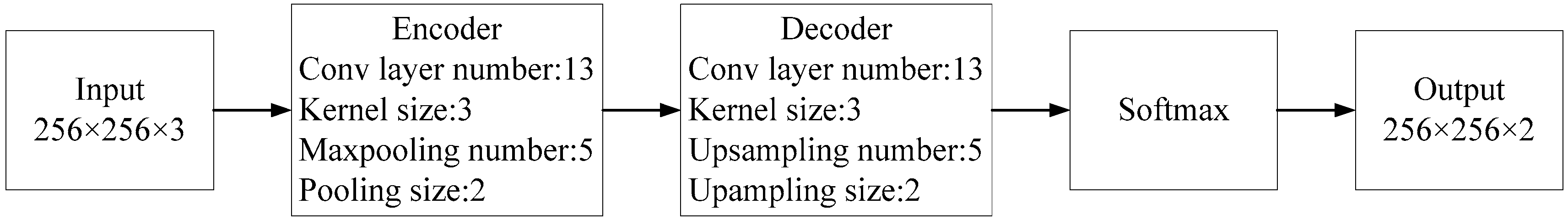
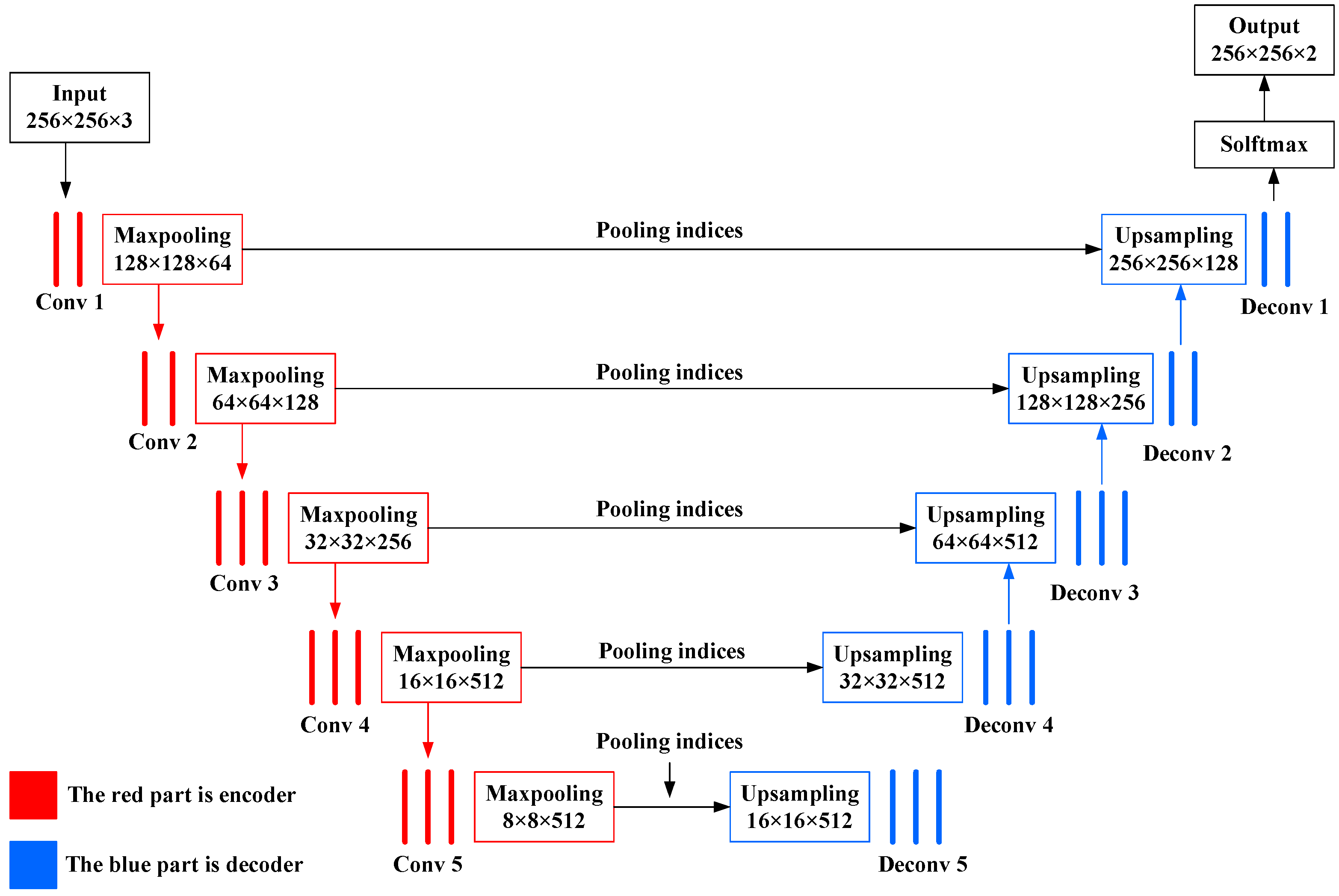
Article

Dark Spot Detection in SAR Images of Oil Spill Using Segnet

Information Science and Technology College, Dalian Maritime University, Dalian 116026, China
*
Authors to whom correspondence should be addressed.
Appl. Sci. 2018, 8(12), 2670; https://doi.org/10.3390/app8122670
Submission received: 15 November 2018 / Revised: 7 December 2018 / Accepted: 16 December 2018 / Published: 18 December 2018
(This article belongs to the Special Issue Intelligent Imaging and Analysis)

Abstract

:
Damping Bragg scattering from the ocean surface is the basic underlying principle of synthetic aperture radar (SAR) oil slick detection, and they produce dark spots on SAR images. Dark spot detection is the first step in oil spill detection, which affects the accuracy of oil spill detection. However, some natural phenomena (such as waves, ocean currents, and low wind belts, as well as human factors) may change the backscatter intensity on the surface of the sea, resulting in uneven intensity, high noise, and blurred boundaries of oil slicks or lookalikes. In this paper, Segnet is used as a semantic segmentation model to detect dark spots in oil spill areas. The proposed method is applied to a data set of 4200 from five original SAR images of an oil spill. The effectiveness of the method is demonstrated through the comparison with fully convolutional networks (FCN), an initiator of semantic segmentation models, and some other segmentation methods. It is here observed that the proposed method can not only accurately identify the dark spots in SAR images, but also show a higher robustness under high noise and fuzzy boundary conditions.

Graphical Abstract

1. Introduction

Due to the influence of short gravity waves and capillary waves on the sea surface, Bragg scattering of the sea surface is greatly weakened, causing the oil film to produce dark spots on synthetic aperture radar (SAR) images [1]. Solberg et al. pointed out that SAR oil spill detection includes three steps: (1) dark spot detection; (2) feature extraction; and (3) discrimination of oil slicks and lookalikes [2]. Among them, the accuracy of dark spot detection is bound to affect the extraction of oil spill location and area. However, some natural phenomena (such as waves, ocean currents, and low wind belts, as well as human factors) may change the backscatter intensity on the surface of the sea, thus leading to an uneven intensity, high noise, or blurred boundaries of oil slicks or lookalikes, making the automatic segmentation of the oil spill area sometimes very difficult. Therefore, a robust and accurate segmentation method plays a crucial role in monitoring oil spills.
There are many studies on dark spot detection on SAR images of oil spill, among which the most widely used method is based on pixel grayscale threshold segmentation, such as a manual single threshold segmentation [3], an adaptive threshold segmentation method [4], and some double threshold segmentation methods [5]. Those methods have simple principles and fast implementation speeds, but they are easily affected by speckle noise and global gray unevenness, thus reducing the accuracy of dark spot recognition. The active contour models (ACM) are another common image segmentation method [6,7]. Compared with traditional segmentation methods, the smooth and closed contours can be obtained by ACM. The most famous and widely used region-based ACM is the borderless ACM proposed by Chan and Vese [7]. The Chan-Vese model performs well in processing images with weak edge and noise, but it cannot process images with uneven intensity and high speckle noise.
With the popularization of neural networks and machine learning algorithms, some studies have used these methods for dark spot detection. Topouzelis et al. proposed a fully connected feed forward neural network to monitor the dark spots in an oil spill area, and obtained a very high detection accuracy at that time [8]. Taravat et al. used a Weibull multiplication filter to suppress speckle noise, enhance the contrast between target and background, and used a multi-layer perceptron (MLP) neural network to segment the filtered SAR images [9]. Taravat et al. also proposed a new method to distinguish dark spots from the combination of the Weibull multiplication model (WMM) and pulse coupled neural networks (PCNN) [10]. Singha used artificial neural networks (ANN) to identify the characteristics of oil slicks and lookalikes [11]. Although this method improved the segmentation accuracy to some extent and suppressed the influence of speckle noise on dark spot extraction, it still cannot obtain high segmentation accuracy and robustness. Jing et al. discussed the application of fuzzy c-means (FCM) clustering in SAR oil spill segmentation, in which it is easy to generate fragments in the segmentation process due to speckle noise images [12]. To suppress the influence of speckle noise on SAR image segmentation of an oil spill, Teng et al. proposed a hierarchical clustering-based SAR image segmentation algorithm, which effectively maintained the shape characteristics of oil slicks in SAR images using the idea of multi-scale segmentation [13]. However, its ability to suppress speckle noise was not good, and the segmentation of weak boundary region was also not ideal.
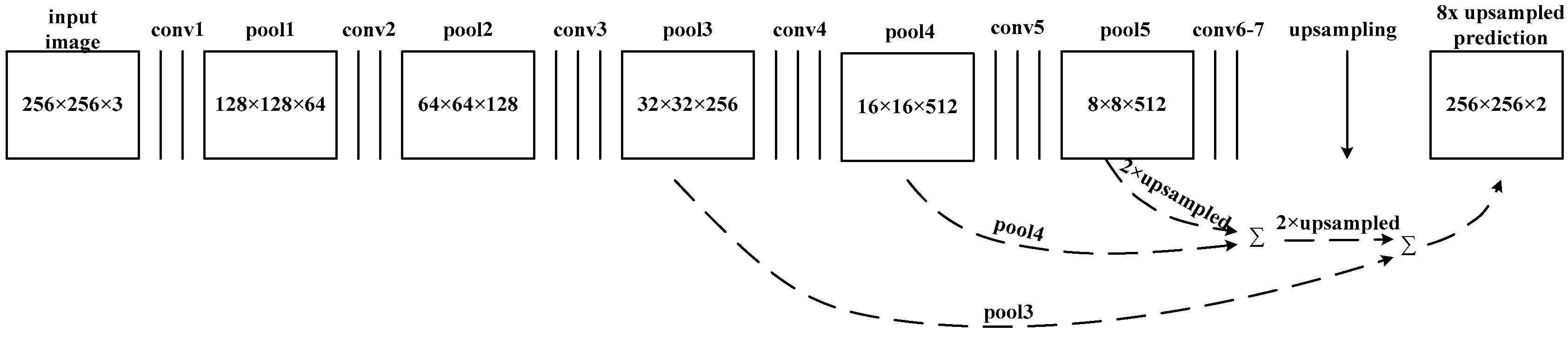
In recent years, deep learning methods have been successfully applied in extracting high level feature representations of images, especially in semantic segmentation. Long et al. changed the full connection layer of the traditional convolution neural networks (CNN) for pixel-based classification [14]. Persello et al. used fully convolutional networks (FCN) to improve the detection accuracy of informal residential areas in high-resolution satellite images [15]. Huang et al. successfully applied the FCN model to weed identification in paddy fields [16]. However, FCN is not sensitive to the details in the images, and its up-sampling results are often blurred. Badanlayan et al. proposed a classic deep learning method (i.e., Segnet) for image semantic segmentation, which was used for automatic driving or intelligent robots [
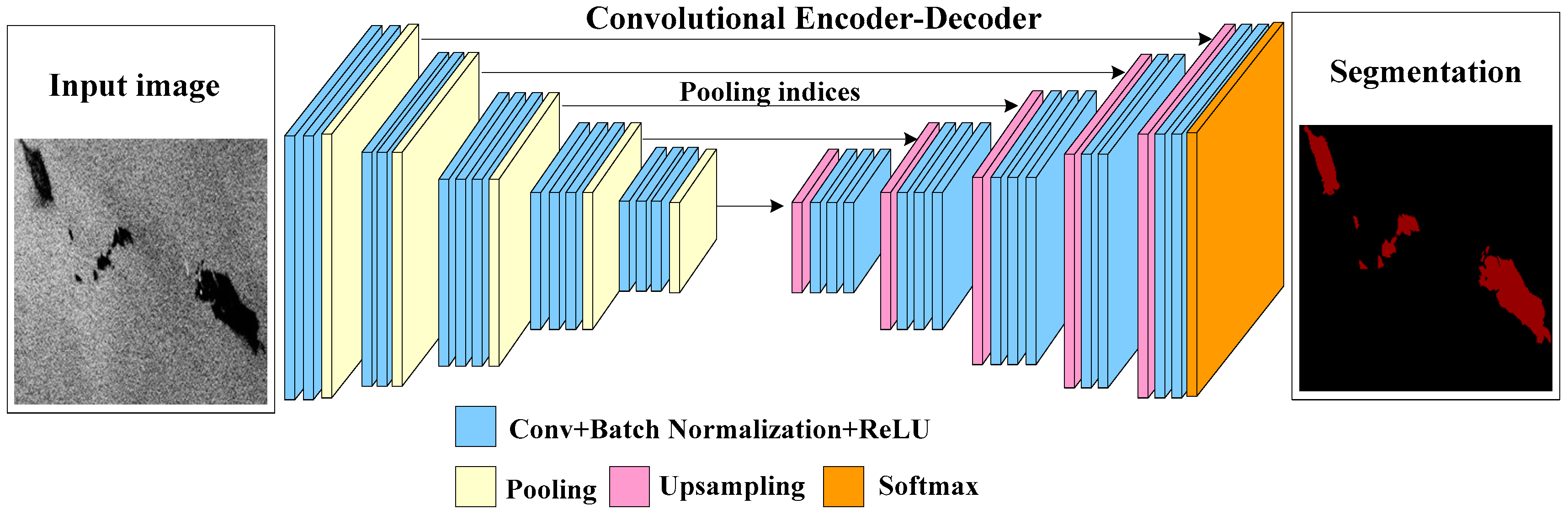
17]. The model has obvious advantages over FCN in storage, calculation time, and segmentation accuracy.
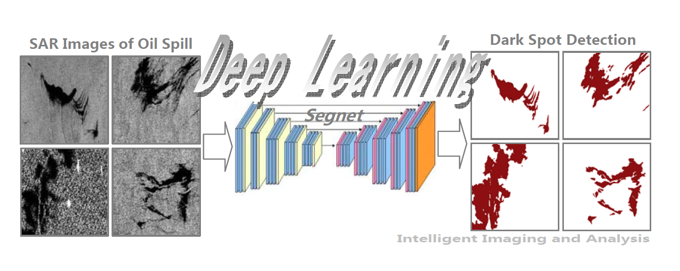
Inspired by the great success of Segnet in image semantic segmentation [17,
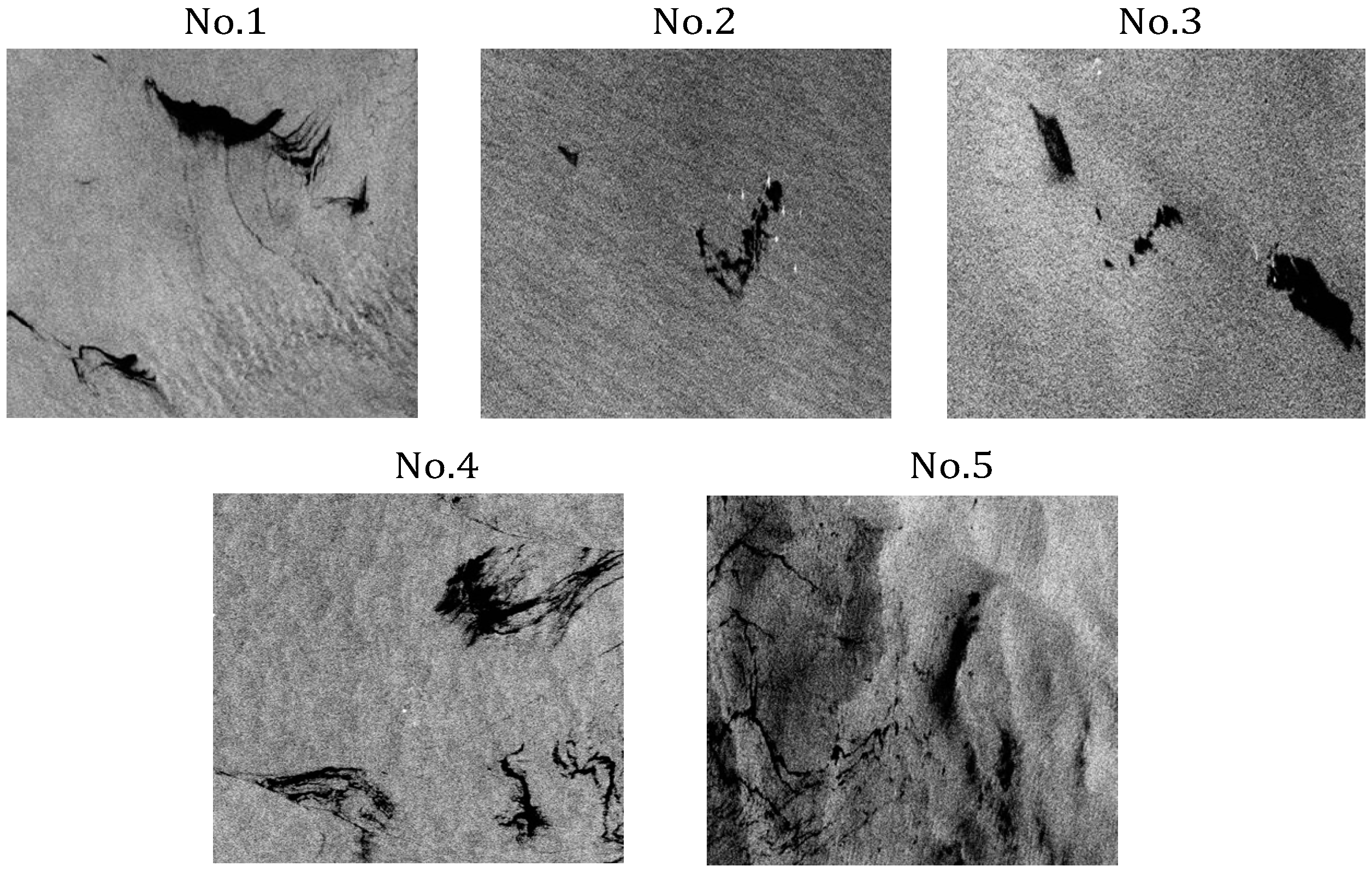
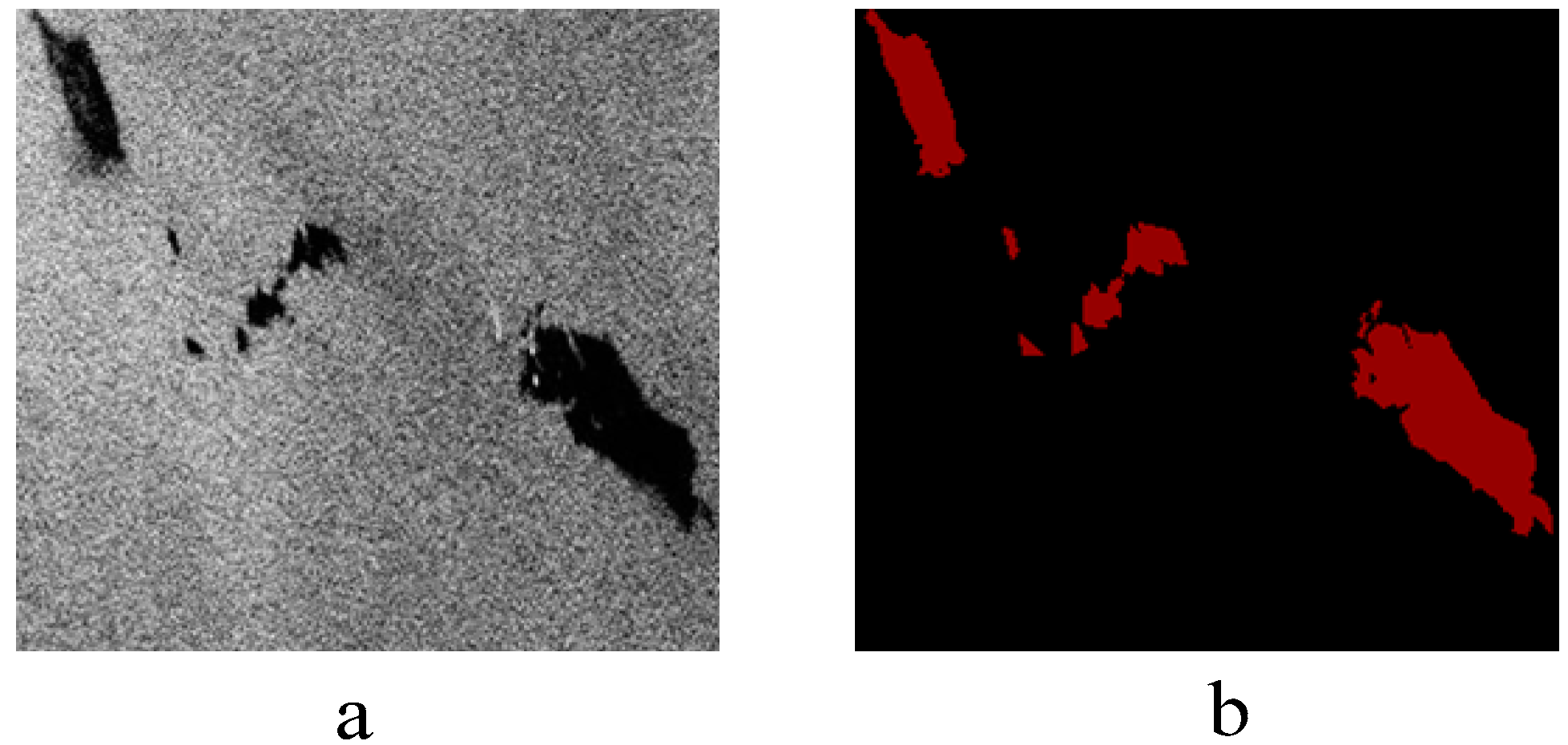
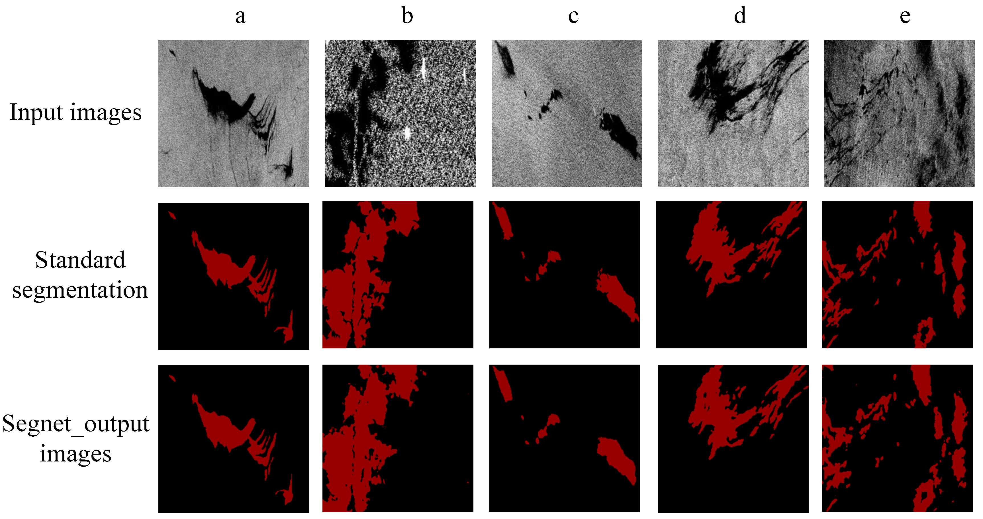
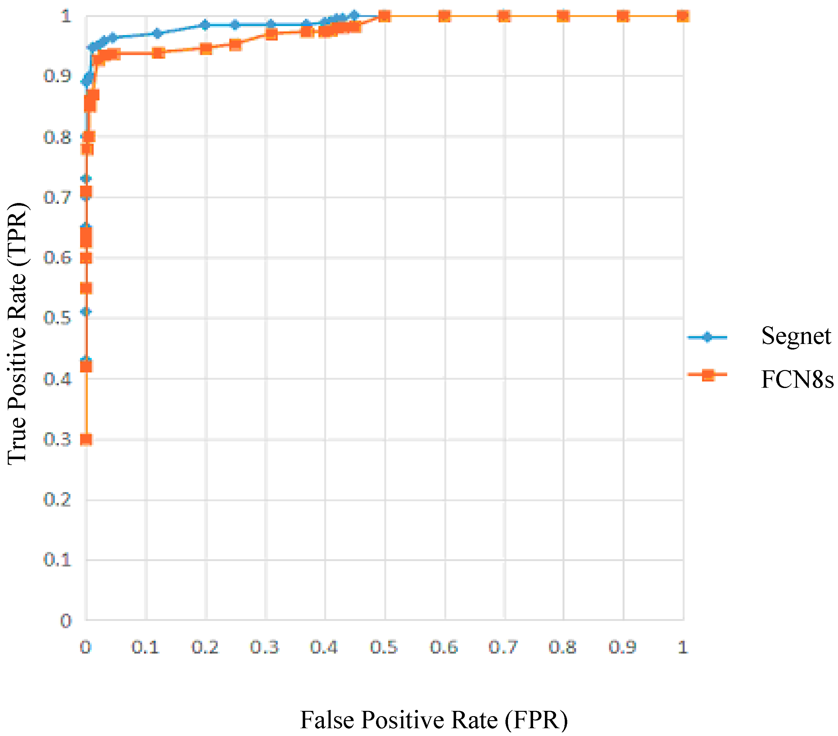
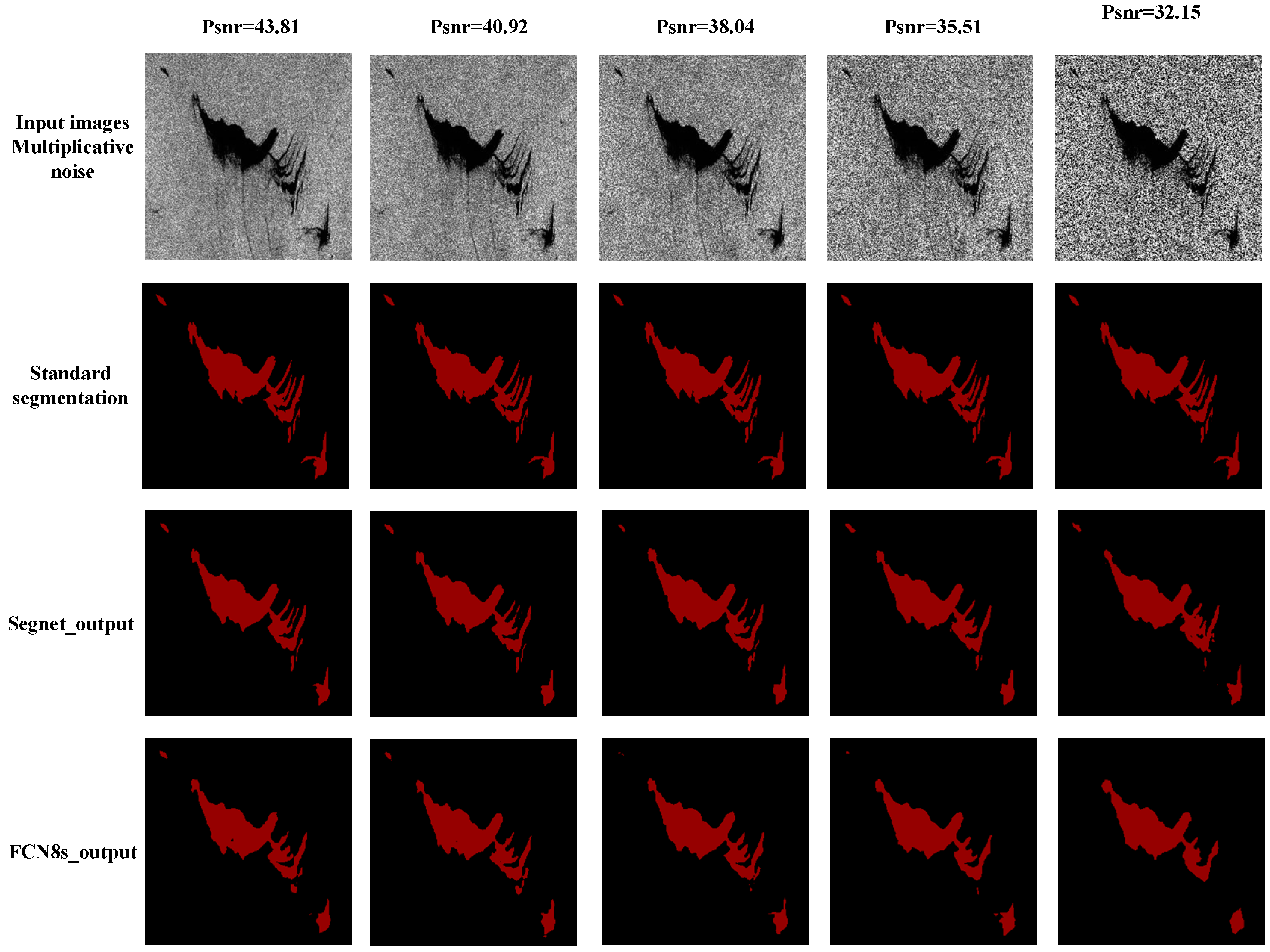
18], we used Segnet as a segmentation model to detect dark spots in oil spill areas. The proposed method is applied to a data set of 4200 from five original SAR images of oil spill. Each scene image is cropped according to four different window sizes, and samples containing oil slicks and seawater are selected from the cropped pieces as data sets. Four hundred and twenty samples were selected from each oil slick scene, with a total of 2100 sample data. To enhance the robustness of the training model, 21 samples in each oil slick scene were added with 10 noise levels of multiplicative and additive noise, respectively, totaling 2100 noisy images. The training set consisted of 1800 original samples and 1800 noisy samples, totaling 3600. The testing set consisted of 600 samples, including 300 original samples and 300 sets of noisy samples (20 noise level data corresponding to three samples randomly selected in each oil slick scene). The effectiveness of the method is demonstrated through the comparison with FCN and some classical segmentation methods (such as support vector machine (SVM), classification and regression tree (CART), random forests (RF), and Otsu, etc.). The segmentation accuracy based on Segnet can reach 93.92% under high noise and weak boundary conditions. It is here observed that the proposed method can not only accurately identify the dark spots in SAR images, but also show higher robustness.
The rest of this paper is organized as follows. Section 2 focuses on the preparation process of the data set, which includes description, preprocessing, and sampling of five SAR oil slick scenes acquired by C-band Radarsat-2. In Section 3, we describe the segmentation based on the Segnet model and the parameter selection in the training process. The validity of the algorithm is verified through analysis and compared with the experimental results of the semantic segmentation model FCN8s. In Section 4, we analyze the validity and stability of the model. The conclusions and outlooks are discussed in the final section.

2. Study Area and Data Sets

2.1. Study Area and Pretreatment

Five SAR oil slick scenes acquired by Radarsat-2 (fine quad-polarized mode) are described in Table 1, and some information on those data (e.g., wind direction, water temperature, etc.) is described in detail in Guo’s studies [19]. Radarsat-2 images of the Mexico Bay area (No.1 and No.4) were acquired on 8 May 2010 and 24 August 2011, respectively. The dark spots in Figure 1 were interpreted as crude oil. North Sea of Europe area data sets (No.2 and No.3) were acquired from 6–9 June 2011. There are three substances (i.e. crude oil, oil emulsion, and plant oil) in the two scenes, and the acquisition interval of No.2 and No.3 was about 12 hours. The data No.5 was obtained in the South China Sea on 18 September 2009. The experimental data contain a small amount of crude oil and plant oil, which were poured with 15-minute intervals.
Quad-polarization SAR images are susceptible to noise. Pauli decomposition has the advantages of anti-interference and a general high adaptability [20]. In general, the Pauli decomposition images are clearer than original quad-polarization SAR images. The image preprocessing stages are as follows:
(1)
The original quad-polarization SAR data are decomposed by Pauli.
(2)
The obtained Pauli decomposition images are filtered by 3 × 3 Boxcar filtering.

2.2. Sampling Process

The Vapnik-Chervonenkis (VC) dimension is usually used to predict the probability of testing errors of models. Vapnik [21] proves that the probability of the upper bound of the testing error is given by (1):
Pr ( t e s t i n g e r r o r t r a i n i n g e r r o r + 1 N [ D ( log ( 2 N D ) + 1 ) log ( η 4 ) ] ) = 1 η
where D is the VC dimension of the classification model. N is the number of training samples. 1 N ( [ D ( log ( 2 N D ) + 1 ) log ( η 4 ) ] ) is also called the model complexity penalty. When the testing error is less than the training error plus the model complexity penalty, the probability is 1 η . The bigger the D , the bigger the model complexity penalty, and the bigger the N , the smaller the model complexity penalty. Generally speaking, a deep learning model needs enough samples. Otherwise, the generalization of the model would be limited, i.e., over-fitting.
The proposed method was applied to a data set of 4200 samples from five original SAR images of oil spill. Here, the data set was processed by the following steps and was called the OIL_SPILL_DATASET:
(1)
In order to ensure that each sampling window includes oil slicks and seawater, the window size cannot be too small or too large, and the window sizes were selected to be 500 × 500 , 1000 × 1000 , 1500 × 1500 , and 2000 × 2000 for each scene of the quad-polar SAR image, respectively. Samples, including oil slicks and seawater, were selected from those sub-images, 420 samples were selected from each scene data, totaling 2100 samples. The boundary complexity and weak boundary were the main factors affecting the segmentation accuracy. The boundary complexity and boundary strength of 420 samples selected from each scene data are shown in detail in Table 2.
(2)
To ensure the balance of the sample distribution, 105 samples (21 samples in each scene) in 2100 samples were added with multiplicative noise and additive noise, respectively, among which multiplicative noise had 10 levels (peak signal-to-noise ratio (PSNR) was between 50 and 30) and additive noise had 10 levels (PSNR was between 50 and 30). A total of 20 different levels of noise were applied to each sample. In this way, the number of samples per scene was extended from 420 to 840, and the total number of samples was up to 4200.
(3)
Due to the limitation of the graphics processing unit (GPU) capabilities, the samples with different sizes obtained in Steps (1) and (2) were resized into 256 × 256 .
(4)
Segnet is a supervised pre-training process, and a label should be made for each sample. In Figure 2b, the black area represents the background (seawater) and the red region represents the target (oil slicks or lookalikes).
(5)
4200 samples were randomly divided into a testing set or a training set according to the ratio of 1:6. To ensure the same distribution of data in the training set and the testing set, 15 samples were selected from 105 samples added with noise, of which three were contained in each oil slick scene. 300 samples of each noise level corresponding to the 15 test samples were selected from the remaining 2100 noisy samples. The testing set contained 600 samples and the training set contained 3600 samples.

3. Dark Spot Detection Using Segnet

3.1. Introduction to Segnet

Segnet is a deep convolution neural network with a sound performance of image semantic segmentation [17]. The basic framework of Segnet is an encoder and a decoder. The most important components of Segnet include a convolution layer, pooling layer, up-sampling layer, and softmax layer, see Figure 3. The encoder consists of the convolution layer, batch normalization layer, and rectified linear unit (ReLU), and its structure is similar to the visual geometry group (VGG)-16 network [22]. The convolution layer is the main component of the encoder, and each output pixel is only linked to the local area of the next input layer, thus forming a local receptive field [23]. The decoder consists of a transposed convolutional layer and an up-sampling layer, and its structure is symmetrical to that of the encoder. The convolution layer corresponds to the transposed convolution layer and the max pooling layer corresponds to the up-sampling layer [24]. At the end of the decoder, the category of each pixel is output through a softmax layer.
The training process of Segnet can be summarized as follows:
(1)
Each sample in the training set and its corresponding label are input into the Segnet in sequence.
(2)
The cross loss entropy is used as the objective function of the training model, and its value is calculated by weighted average for all pixels in each training sample [17].
(3)
Through the back propagation algorithm, the weights are updated according to the minimum error.
The information in Steps (1) and Steps (2) is forward propagating, and the outputs are obtained by convolution of inputs and weights. Step (3) is the backward propagation process. According to the results of Step (2), the weights are passed to the previous layers through the backward propagation algorithm, and the weights are updated.

3.2. Image Segmentation of Oil Spill Using Segnet

Segnet is an end-to-end training process. In this experiment, the training process of the Segnet was based on 3600 training samples, of which 1800 were original images, 900 were additive noise images, and 900 were multiplicative noise images. Due to limitations of the GPU capabilities, one sample at a time was input during the training process. Here, the epoch was set at 30, and the fixed learning rate was 0.01.
The structure and parameters of Segnet are shown in Figure 4. The application of Segnet excluding the batch normalization layer is shown in Figure 5. The training performance diagram of Segnet is shown in Figure 6. In our study, the weight initialization process of the encoder and decoder was based on the research of He et al. [25]. When the learning rate is 0.0001, the training loss would be relatively large. When the learning rate is 0.001, the training would be relatively stable soon, but it is not as good as the training performance when the learning rate is 0.01.
Parts of of the test results of Segnet model based on the OIL_SPILL_DATASET are shown in Figure 7. Where a, b, c, d, and e are representative samples of five boundary statuses, respectively, and a brief description of the five boundary statuses is shown in Table 3. It can be seen from Figure 7 that Status-a (medium boundary complexity) and Status-c (ideal boundary) achieved the best segmentation results in the five boundary statuses, and Status-b (strong noise) and Status-d (complex boundary) were slightly inferior. For Status-e (weak boundary), the Segnet can still effectively segment dark spots in general, although some backgrounds were incorrectly segmented into dark spots.
We used a trained model to test samples with a learning rate of 0.01. The segmentation results did not achieve the expected results (seeing Figure 8). For the samples without noise or with low multiplicative and additive noise in the testing set, the segmentation effect was good. However, almost all pixels with high additive noise were predicted as the background. To reduce the computational and storage pressure of GPU, we chose a Segnet’s batch size of 1 (i.e., inputting one sample at a time), and found that in this case, the Segnet can achieve a better segmentation effect without using the batch normalization layer [26]. Finally, the learning rate was 0.01, and the batch normalization layer was removed based on the basic structure of Segnet.

3.3. Comparison of Segnet to FCN

Three end-to-end FCN models (i.e., FCN32s, FCN16s, and FCN8s) were proposed by Long et al. [14], among which FCN8s (8-step sampling) was considered the best one. The FCN8s encoder includes convolution layers with a 3 × 3 convolution kernel. The convolution layers changed from the last three full connection layers are convolution kernels of 7 × 7 , 1 × 1 , 1 × 1 , and the convolution layers of layers 6–7 are all characteristic images 1 × 1 × 4096 . The last de-convolution layer can be considered as an up-sampling process, which can be used to obtain the segmentation image with the same size as the original image. The up-sampling process of FCN8s is a jump architecture, which performs up-sampling on the results of different pool layers of pool 3, pool 4, and pool 5, and then optimizes the output according to these results. The size of the output picture was the same as that of the input, and its number of channels was 2, which indicates that the output prediction picture contained two categories (seawater and oil slicks). A schematic diagram of FCN8s’ model operation is given in Figure 9.
In our study, the FCN8s’ structure did not include the batch normalization layer. We tested some learning rates (0.01, 0.001, 0.0001) during FCN8s’ training and found that the required accuracy could be obtained when the learning rate was 0.001, but the cost was a longer training period than Segnet. The training parameters of FCN8s and Segnet are shown in Table 4. The training performance of FCN8s is shown in Figure 10. When epoch reached 10, the training loss was close to 0.06 and tended to be stable.
The comparison between Segnet and FCN8s is shown in Figure 11, and the five samples (a–e) represent the boundary statuses, respectively (see Table 3). The results show that FCN8s has a good overall segmentation effect. However, the performance needs to be improved in oil spill images with weak boundaries and high boundary complexity. The Sample-d and Sample-e are both high wind speed regions in Figure 11. Due to the high wind speed, the oil slick boundary complexity in Sample-d was high, and the segmentation results were not ideal.
The receiver operating characteristic (ROC) analysis was used to evaluate the proposed algorithm with the pixel classification accuracy of FCN8s. Since our model input was a sample containing both oil slicks and seawater, it was difficult to ensure that the pixel ratio of oil slicks and seawater was 1:1. To ensure that the pixel ratio of oil slicks and seawater was as close as possible to 1:1, we re-selected the training set and the testing set. According to the label of each sample in the training set, the number of pixels of oil slicks and seawater in each sample was calculated, respectively, and finally, 2800 pieces of data with the pixel-to-pixel ratio of oil slicks and seawater of 0.998:1 were selected. The testing set selected 200 test data with a ratio of 0.989: 1 from 600 testing sets. The ratio of the training set to testing set was still 6:1. The ROC curves for Segnet and FCN8s are shown in Figure 12, and we can see that the ROC curves of Segnet and FCN8s are very close to the upper left corner, but there are still some differences. Under the condition of a high false positive rate (FPR), both showed a higher true positive rate (TPR). However, under the condition of low FPR, the TPR of FCN was lower than that of Segnet. The results show that Segnet has achieved a moderate TPR in the whole range of FPR.

4. Analysis of Segmentation Experiments

4.1. Efficiency Analysis

We compared the performance of FCN8s and Segnet from the following four aspects: Pixel-classification accuracy (PA), mean accuracy (MA), mean intersection over union (MIoU), and frequency weighted intersection over union (FWIoU). The comparison of the four standard values for FCN8s and Segnet with five boundary statuses (see Table 3) is shown in Figure 13. It can be observed that the performance of Segnet and FCN8s for the first four boundary statuses was almost the same, and the PA was above 95%. However, for Status-e (Weak boundary strength), Segnet was superior to FCN8s in the segmentation effect, and the PA of Segnet reached 93.92%. FCN8s performed slightly worse for weak boundary segmentation, achieving 87.53% of PA. Thus, that Segnet can effectively detect dark spots (oil slicks or lookalikes) in SAR images.

4.2. Stability Analysis

Due to the influence of the sea surface environment (such as waves, ocean currents, and low wind belts) and the characteristics of SAR sensors, high noise and weak boundaries are commonly found in SAR images of oil spill. Figure 14 shows an example of the segmentation effect of a test sample at five additional noise levels. The first row is a SAR test sample with five different peak signal-to-noise ratio (PSNR), and the second row is the label of each sample. The outputs of Segnet and FCN8s are listed in the third and fourth rows, respectively. Figure 15 shows the segmentation effect of the same test sample at five multiplicative noise levels.
Correspondingly, the effectiveness of the proposed method is demonstrated through the analysis of some experimental results. The same training set and test set were applied to FCN8s and some classical image segmentation methods, such as SVM, CART [27], RF [28], and Otsu. The four aforementioned evaluation parameters (PA, MA, MIoU, and FWIoU) at 10 additive noise levels are shown in Figure 16, and a comparison at 10 multiplicative noise levels is shown in Figure 17, where the X coordinate is PSNR. We can see the following trend:
(1)
In addition to some fluctuations of MA of Segnet where PSNR is relatively large in Figure 16, the other three parameters (PA, MIoU, and FWIoU) are basically on a horizontal line, which proves that Segnet shows high robustness in terms of additive noise.
(2)
When PSNR is generally less than 35 in Figure 16, all four indicators of FCN8s have a clear downward trend, which indicates that FCN8S is not as stable as Segnet when the additive noise is relatively high.
(3)
In Figure 16, the four classical segmentation methods (SVM, CART, RF, and Otsu) are sensitive to additive noise (especially when PSNR is generally less than 35), and the comparison of the three indicators (MA, MIoU, and FWIoU) shows that they are not as good as Segnet and FCN8s. Although these three methods (SVM, CART, and RF) seem to have a similar performance with Segnet and FCN8s based on PA, this phenomenon should be related to PA’s defects. It is very difficult to ensure that oil slicks and seawater have the same initial probability in the testing set.
(4)
In Figure 17, Segnet and FCN8s show high stability and tolerance to multiplicative noise, although the overall performance of FCN8s is not as good as that of Segnet. When PSNR is less than 35, the PA of FCN8s is obviously decreased.
(5)
The four classical segmentation methods (SVM, CART, RF, and Otsu) are much more sensitive to multiplicative noise than Segnet and FCN8s, especially when the noise is high, and the performance of those classification methods drops sharply. In addition, Otsu’s performance is significantly worse than the other three methods.
Overall, by comparing the four parameters (PA, MA, MIoU, and FWIoU) of the additive and multiplicative noise in Figure 16 and Figure 17, the traditional machine algorithm performed poorly in detecting dark spots compared with semantic segmentation algorithms. Table 5 shows the comparison of segmentation accuracy (averages values of PA, MA, MIoU, and FWIoU) and running time (GPU time) using the same test set (600 samples). Due to the complex structure of the deep learning model, its running time was much longer than that of the classical machine learning model.

4.3. Overfitting Analysis

The initial probability of the data in the overfitting experiment was equal. For the first experimental model, the training samples were from the first three SAR oil slick scenes (No.1–No.3). The number of samples from each scene was 720, and the total number of training samples was 2160. The training data of the second experimental model included 720 samples selected from the first SAR oil slick scene (No.1) only. The two models were tested using the same test data, and those 120 test samples here were selected from the SAR oil slick scenes (No.1). The training set of the first model contained 1080 original samples and 1080 noise samples. Accordingly, the training set of the second training model included 360 original samples and 360 noise samples, which have the same distribution as that of the first model. The average values of each parameter based on the first and second models are shown in Table 6, and the average values of the four parameters of the second model were higher than that of the first model. It can be seen that there is indeed an over-fitting phenomenon when the sample space is insufficient.

4.4. K-Fold

K-fold cross validation (K-CV) can effectively avoid over-fitting and under-fitting [29]. The data set is randomly divided into K groups to verify the validity of the training model. Each subset of the data set is used as a testing set and the remaining K-1 groups are used as training sets. On the basis of K-CV, we verified the performance of the model by using the mean and variance of PA. K = 3, 5, 7, and 9 are shown in Table 7. With the improvement of PA, the stability of the model would be improved. When K increased to 7, the increase of PA and variance tended to be stable. Here, K was set to 7 in consideration of statistical stability and calculation costs. Therefore, the ratio of the testing set to training set was 1:6, the total data set had 4200 samples, the testing set had 600 samples, and the training set contained 3600 samples.

5. Conclusions and Outlooks

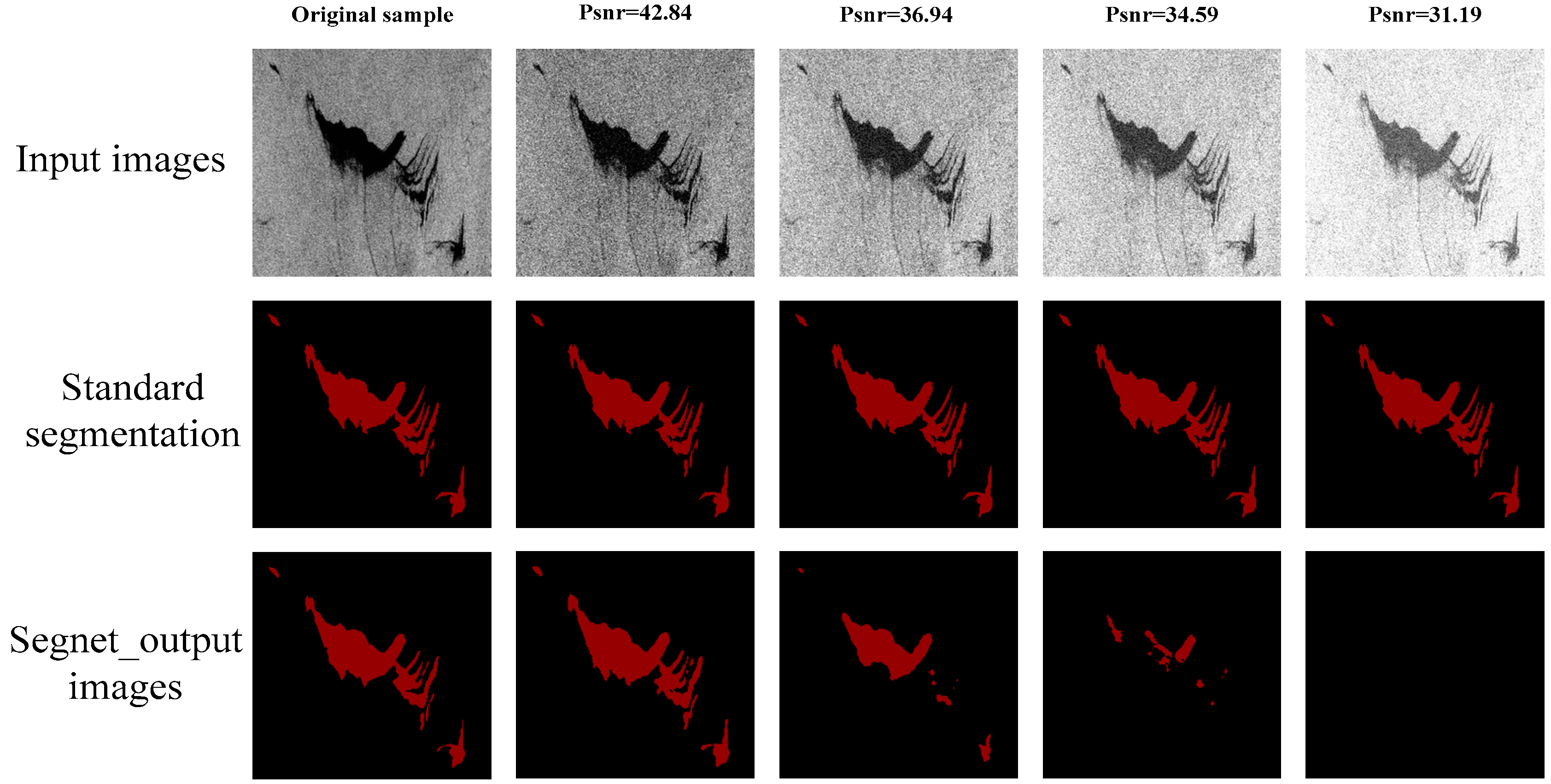
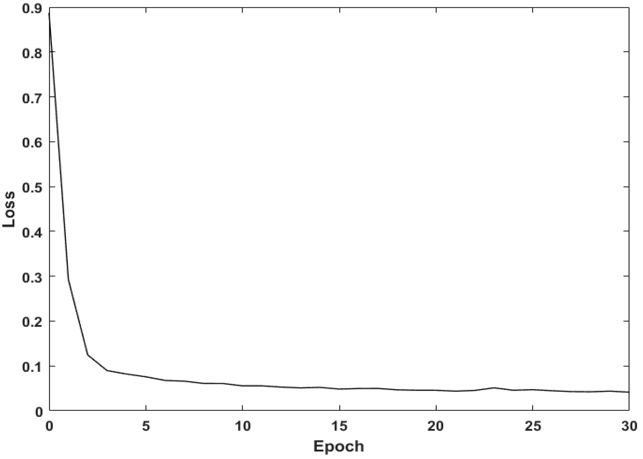
The current research used Segnet to extract dark spots in SAR images of an oil spill. To reduce the computational and storage pressure of GPU, we chose a Segnet’s batch size of 1 (i.e., inputting one sample at a time), and found that in this case, the Segnet achieved a better segmentation effect without using the batch normalization layer. The proposed method effectively distinguished between oil slicks and seawater based on the data set (OIL_SPILL_DATASET), and high accuracy segmentation results were obtained for SAR images with high noise and weak boundaries.
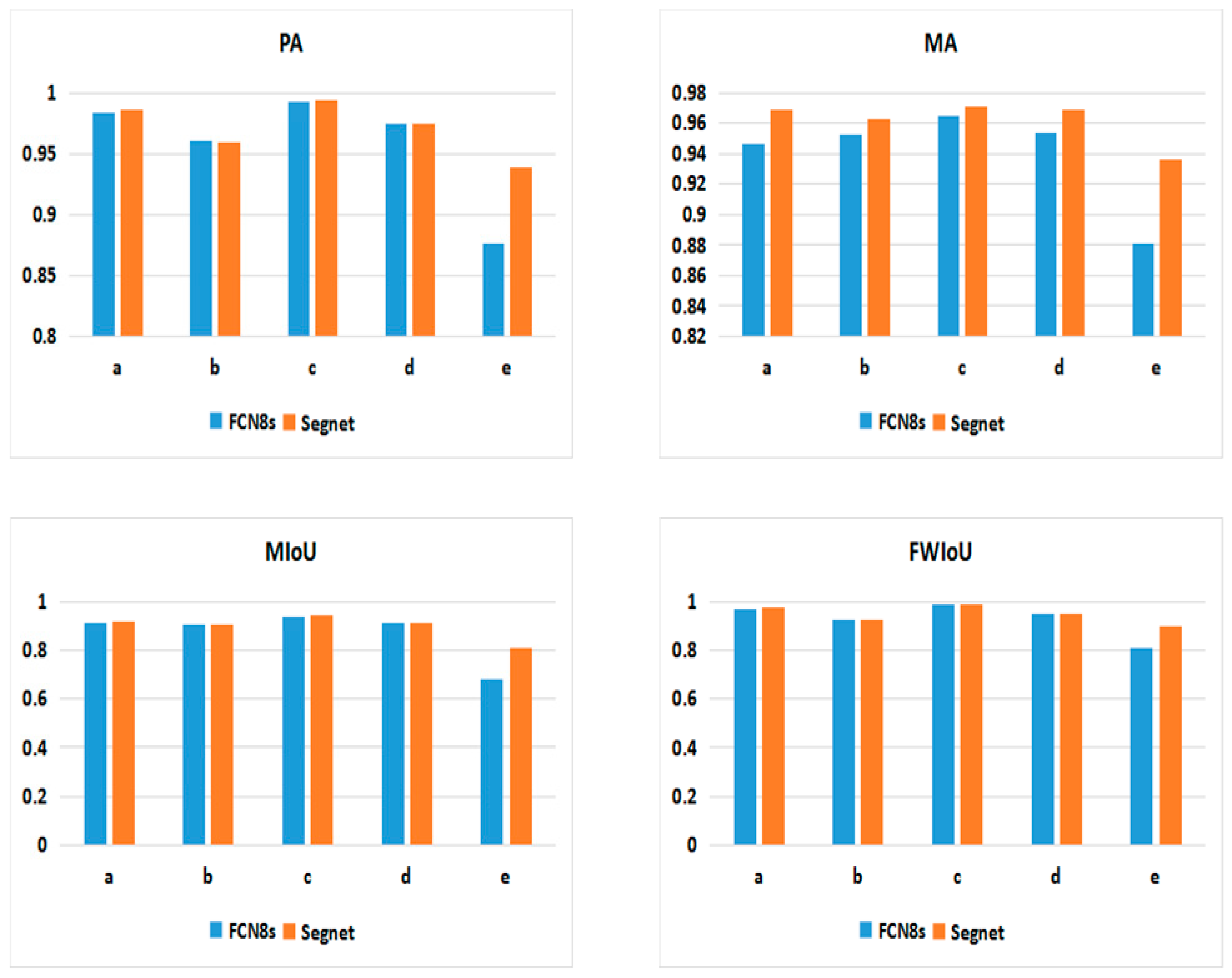
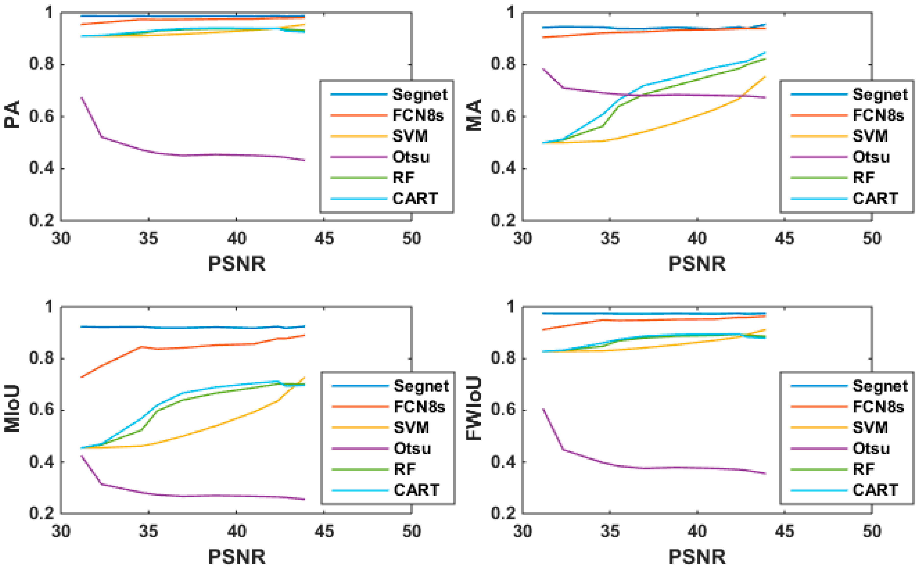
The OIL_SPILL_DATASET was also applied to FCN8s and some other classical segmentation methods. By comparing the four parameters (PA, MA, MIoU, and FWIoU) of different addition and multiplication noise levels, the following trends were found:
  • Segnet and FCN8s showed high stability and tolerance to addition and multiplicative noise, although the overall performance of FCN8s was not as good as that of Segnet. In addition, Segnet was obviously superior to FCN8s in weak boundary regions.
  • Some classical segmentation methods (such as SVM, CART, RF, and Otsu) were much more sensitive to addition and multiplicative noise than the deep learning models.
However, Segnet’s training process was supervised, and its training relies on a large number of label images. The production of labels was not only time-consuming and laborious in the data preparation stage, but also the training effect could be easily affected by human factors. In the future, we hope to shift to a weak or unsupervised training process to improve the convenience of application.

Author Contributions

H.G. conceived and designed the algorithm, and constructed the outline for the manuscript; G.W. performed the experiments, analyzed the data, and made the first draft of the manuscript; J.A. was responsible for determining the overall experimental plan, and polished the manuscript.

Funding

The work was carried out with the supports of the National Natural Science Foundation of China (Grant 61471079) and State Oceanic Administration of China for ocean nonprofit industry research special funds (No.2013418025).

Conflicts of Interest

The authors declare no conflict of interest. The founding sponsors had no role in the design of the study; in the collection, analyses, or interpretation of data; in the writing of the manuscript, and in the decision to publish the results.

References

  1. Yin, J.; Yang, J.; Zhou, Z.S. The Extended Bragg Scattering Model-Based Method for Ship and Oil-Spill Observation Using Compact Polarimetric SAR. IEEE J. Sel. Top. Appl. Earth Obs. Remote Sens. 2015, 8, 3760–3772. [Google Scholar] [CrossRef]
  2. Solberg, A.H.S.; Brekke, C.; Husoy, P.O. Oil Spill Detection in Radarsat and Envisat SAR Images. IEEE Trans. Geosci. Remote Sens. 2007, 45, 746–755. [Google Scholar] [CrossRef]
  3. Bern, T.I.; Wahl, T.; Andersen, T. Oil Spill Detection Using Satellite Based SAR: Experience from a Field Experiment. Photogramm. Eng. Remote Sens. 1993, 59, 423–428. [Google Scholar]
  4. Solberg, A.H.S.; Storvik, G.; Solberg, R. Automatic detection of oil spills in ERS SAR images. IEEE Trans. Geosci. Remote Sens. 1999, 37, 1916–1924. [Google Scholar] [CrossRef]
  5. Kanaa, T.F.N.; Tonye, E.; Mercier, G. Detection of oil slick signatures in SAR images by fusion of hysteresis thresholding responses. In Proceedings of the 2003 IEEE International Geoscience and Remote Sensing Symposium, Toulouse, France, 21–25 July 2003; pp. 2750–2752. [Google Scholar]
  6. Li, C.; Kao, C.Y.; Gore, J.C. Minimization of Region-Scalable Fitting Energy for Image Segmentation. IEEE Trans. Image Process. 2008, 17, 1940–1949. [Google Scholar] [PubMed] [Green Version]
  7. Chan, T.F.; Vese, L.A. Active Contours without Edges; IEEE Press: New York, NY, USA, 2001. [Google Scholar]
  8. Topouzelis, K.; Karathanassi, V.; Pavlakis, P. Oil spill detection: SAR multiscale segmentation and object features evaluation. Int. Symp. Remote Sens. 2003, 4880, 77–87. [Google Scholar]
  9. Taravat, A.; Oppelt, N. Adaptive Weibull Multiplicative Model and Multilayer Perceptron neural networks for dark-spot detection from SAR imagery. Sensors 2014, 14, 22798–22810. [Google Scholar] [CrossRef] [PubMed]
  10. Taravat, A.; Latini, D.; Frate, F.D. Fully Automatic Dark-Spot Detection from SAR Imagery with the Combination of Nonadaptive Weibull Multiplicative Model and Pulse-Coupled Neural Networks. IEEE Trans. Geosci. Remote Sens. 2014, 52, 2427–2435. [Google Scholar] [CrossRef]
  11. Singha, S.; Bellerby, T.J.; Trieschmann, O. Satellite Oil Spill Detection Using Artificial Neural Networks. IEEE J. Sel. Top. Appl. Earth Obs. Remote Sens. 2013, 6, 2355–2363. [Google Scholar] [CrossRef]
  12. Jing, Y.; An, J.; Liu, Z. A Novel Edge Detection Algorithm Based on Global Minimization Active Contour Model for Oil Slick Infrared Aerial Image. IEEE Trans. Geosci. Remote Sens. 2011, 49, 2005–2013. [Google Scholar] [CrossRef]
  13. Teng-Fei, S.U.; Meng, J.M.; Zhang, X. Segmentation Algorithm for Oil Spill SAR Images Based on Hierarchical Agglomerative Clustering. Adv. Mar. Sci. 2013, 31, 256–265. [Google Scholar]
  14. Long, J.; Shelhamer, E.; Darrell, T. Fully convolutional networks for semantic segmentation. In Proceedings of the IEEE Conference on Computer Vision and Pattern Recognition, Boston, MA, USA, 7–12 June 2015; pp. 3431–3440. [Google Scholar]
  15. Persello, C.; Stein, A. Deep Fully Convolutional Networks for the Detection of Informal Settlements in VHR Images. IEEE Geosci. Remote Sens. Lett. 2017, 14, 2325–2329. [Google Scholar] [CrossRef]
  16. Huang, H.; Deng, J.; Lan, Y. A fully convolutional network for weed mapping of unmanned aerial vehicle (UAV) imagery. PLoS ONE 2018, 13, e0196302. [Google Scholar] [CrossRef] [PubMed]
  17. Badrinarayanan, V.; Kendall, A.; Cipolla, R. SegNet: A Deep Convolutional Encoder-Decoder Architecture for Image Segmentation. IEEE Trans. Pattern Anal. Mach. Intell. 2017, 39, 2481–2495. [Google Scholar] [CrossRef] [PubMed]
  18. Mesbah, R.; McCane, B.; Mills, S. Deep convolutional encoder-decoder for myelin and axon segmentation. In Proceedings of the International Conference on Image and Vision Computing New Zealand, Palmerston North, New Zealand, 21–22 November 2016; pp. 1–6. [Google Scholar]
  19. Guo, H.; Wu, D.; An, J. Discrimination of Oil Slicks and Lookalikes in Polarimetric SAR Images Using CNN. Sensors 2017, 17, 1837. [Google Scholar] [CrossRef] [PubMed]
  20. Yin, H. Classification of polSAR Images Based on Polarimetric Decomposition. Master’s Thesis, University of Electronic Science and Technology of China, Chengdu, China, 2013. [Google Scholar]
  21. Vapnik, V.N. The Nature of Statistical Learning Theory; Springer: Berlin, Germany, 2000. [Google Scholar]
  22. Simonyan, K.; Zisserman, A. Very Deep Convolutional Networks for Large-Scale Image Recognition. arXiv, 2014; arXiv:1409.1556. [Google Scholar]
  23. Wang, J.; Lin, J.; Wang, Z. Efficient Hardware Architectures for Deep Convolutional Neural Network. IEEE Trans. Circuits Syst. I Regul. Pap. 2018, 65, 1941–1953. [Google Scholar] [CrossRef]
  24. Zhang, M.; Hu, X.; Zhao, L. Learning Dual Multi-Scale Manifold Ranking for Semantic Segmentation of High-Resolution Images. Remote Sens. 2017, 9, 500. [Google Scholar] [CrossRef]
  25. He, K.; Zhang, X.; Ren, S. Delving Deep into Rectifiers: Surpassing Human-Level Performance on ImageNet Classification. In Proceedings of the IEEE International Conference on Computer Vision, Santiago, Chile, 11–18 December 2015; pp. 1026–1034. [Google Scholar]
  26. Deep Learning. Available online: http://www.deeplearningbook.org (accessed on 8 April 2016).
  27. Loh, W.-Y. Classification and Regression Trees; John Wiley & Sons: New York, NY, USA, 2011; Volume 1, pp. 14–23. [Google Scholar]
  28. Svetnik, V.; Liaw, A.; Tong, C. Random Forest: A Classification and Regression Tool for Compound Classification and QSAR Modeling. J. Chem. Inf. Comput. Sci. 2003, 43, 1947–1958. [Google Scholar] [CrossRef] [PubMed]
  29. Cross-Validation. Available online: http://blog.sina.com.cn/s/blog_688077cf0100zqpj.html (accessed on 14 October 2011).
Figure 1. Five oil spill RadarSat-2 scenes.
Applsci 08 02670 g001
Figure 2. Label for each sample. (a) An input image; (b) the label of the image.
Applsci 08 02670 g002
Figure 3. The framework of Segnet.
Applsci 08 02670 g003
Figure 4. The structure and parameters of Segnet.
Applsci 08 02670 g004
Figure 5. The application of Segnet without the batch normalization layer.
Applsci 08 02670 g005
Figure 6. Training performance of Segnet based on different learning rates.
Applsci 08 02670 g006
Figure 7. The segment effect of some test samples with different boundary status.
Applsci 08 02670 g007
Figure 8. Comparison of segmentation results with different levels of additive noise.
Applsci 08 02670 g008
Figure 9. The structure and parameters of FCN8s (8-step sampling).
Applsci 08 02670 g009
Figure 10. Training performance of FCN8s (Learning rate is 0.001).
Applsci 08 02670 g010
Figure 11. Comparison of segmentation results of FCN8 and Segnet for five boundary statuses.
Applsci 08 02670 g011
Figure 12. ROC curves of Segnet and FCN8s.
Applsci 08 02670 g012
Figure 13. Comparison of the four evaluation parameters with five boundary statuses.
Applsci 08 02670 g013
Figure 14. Comparison of Segnet and FCN8 with five levels of additive noise.
Applsci 08 02670 g014
Figure 15. Comparison of Segnet and FCN8 with five levels of multiplicative noise.
Applsci 08 02670 g015
Figure 16. Four image segmentation standard values under 10 additive noise levels.
Applsci 08 02670 g016
Figure 17. Four image segmentation standard values under 10 multiplicative noise levels.
Applsci 08 02670 g017
Table 1. Information of the five quad-polarization SAR images of oil spill.
Scene IDNo.1No.2.No.3No.4No.5
Location of Center26°49′N/92°01′W59°59′N/2°25′E60°09′N/2°19′E27°54′N/90°55′W18°06′N/109°25′E
Wind Speed~6.5 m/s1.6–3.3 m/s1.6–3.3 m/s~15 m/s~10 m/s
Types of Dark SpotCrude oilPlant oil/oil emulsionPlant oil/oil emulsion/crude oilCrude oilOil emulsion/crude oil
Sample size420420420420420
Table 2. Sample collection of No.1–No.5.
Boundary Complexity - Boundary StrengthNo.1No.2No.3No.4No.5
Low - Low----190
Low - Moderate----50
Low - High32050420-30
Moderate - Low----130
Moderate - Moderate-140--20
Moderate - High100--60-
High - Low-----
High - Moderate-230- -
High - High---360-
Table 3. Five boundary statuses of oil slicks.
Status IDabcde
Status of boundaryMedium boundary complexity, low noiseStrong noiseIdeal boundaryHigh boundary complexityWeak boundary strength
Number of samples3030303030
Table 4. Training parameters of Segnet and FCN8s.
MethodsLearning RateBatch SizeBatch NormalizationVolatile GPU-UntilGPU Training MemoryModel Size
Segnet0.011off99%1119 MB114 MB
FCN8s0.0011off100%5319 MB537 MB
Table 5. Comparison of the six segmentation methods.
MethodsTime (s)PAMAMIoUFWIoU
Segnet1.639 × 1040.9390.8950.8010.914
FCN8s1.703 × 1040.8840.8050.7830.823
SVM1.353 × 1020.8540.6930.5680.795
Otsu2.192 × 10−30.5730.5430.3750.508
RF1.1830.8670.7350.6120.814
CART2.023 × 10−20.8550.7490.6050.810
Table 6. Evaluation of Segnet and FCN8s based on the four image segmentation standard values.
Training SetAverage PAAverage MAAverage MIoUAverage FWIoU
SegnetFCN8sSegnetFCN8sSegnetFCN8sSegnetFCN8s
No.1–No.30.98450.95890.94370.86440.91740.84190.97240.9481
No.10.98580.96920.9530.89520.92080.86370.97340.9547
Table 7. Mean and variance of pixel-classification accuracy (PA) based on K-CV.
KAverageVariance
30.9666174690.010223167
50.9753051360.001727448
70.9852427570.000513106
90.9861906310.000499049

