Influence of Analyzed Sequence Length on Parameters in Laryngeal High-Speed Videoendoscopy

 , ,
, , 
Abstract
1. Introduction
- Examine if varying sequence length affects GAW perturbation parameters.
- Determine if there is a statistical change in parameters by varying sequence length.
- Investigate the reason for the susceptibility of these parameters to a changing sequence length.
2. Materials and Methods
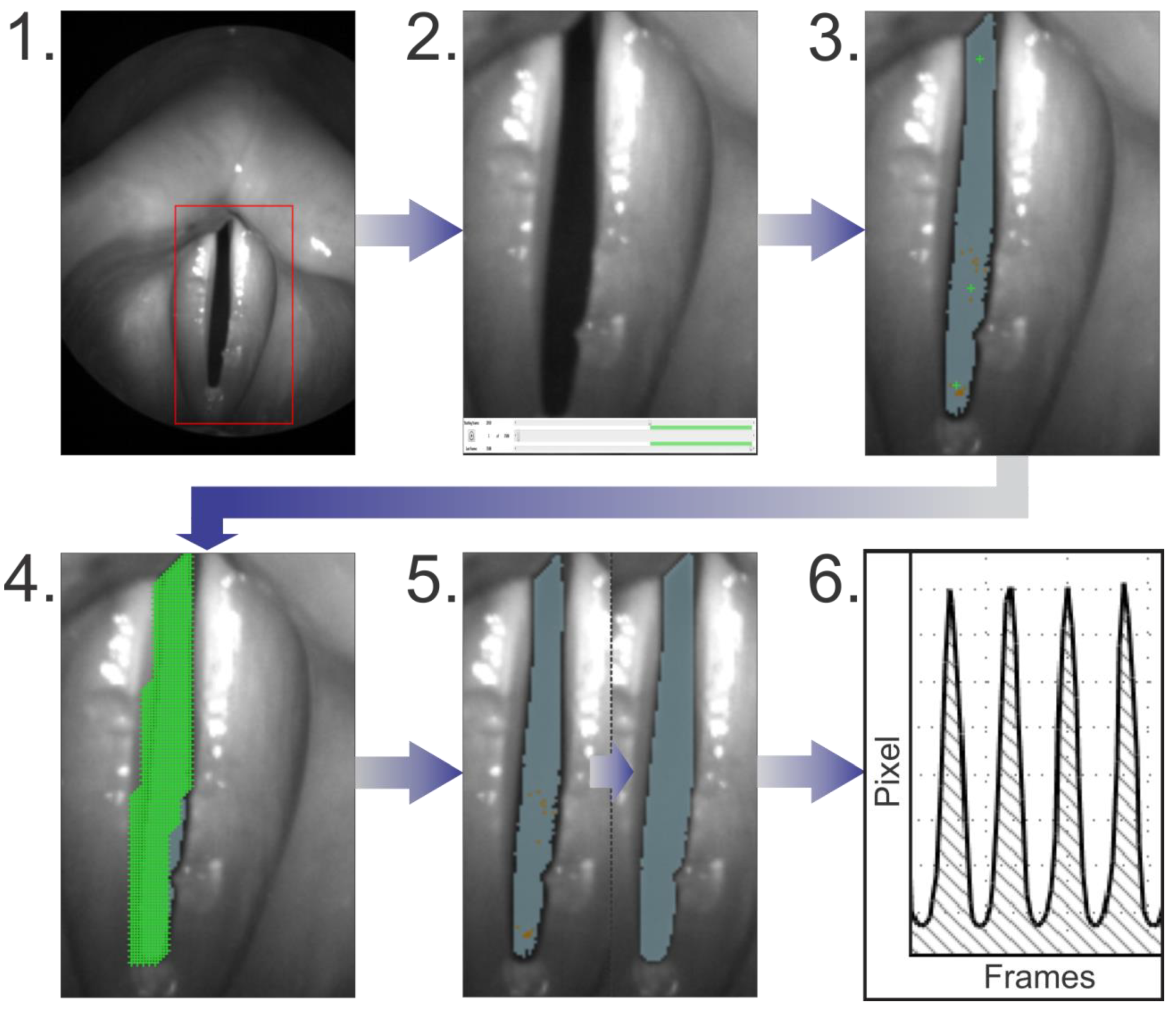
- A region of interest in the video was selected, which included full view of glottis.
- An interval containing at least 102 cycles during constant phonation was selected. When selecting the intervals, care was taken to choose sections in which the glottis was completely visible and the field of view moved as little as possible.
- For the initial pre-segmentation, seed points (green crosses in Figure 2(3,4)) were set and brightness thresholds were used. All pixels surrounding a seed point position including the pixel on the position itself are marked, if they are darker than the selected brightness thresholds.
- Afterwards the seed points were substituted by a regular seed point grid. In the grid region every second pixel was marked with a seed point. The grid was created semi-automatically by using a seed point drawing tool.
- The brightness thresholds were adjusted yielding the finalized brightness settings.
- The total GAW (GAWT) was extracted for each recording.
3. Results
4. Discussion
5. Shortcomings
6. Conclusions
Supplementary Materials
Author Contributions
Funding
Acknowledgments
Conflicts of Interest
Appendix A

| Parameter Name and Sequence Length | Average | Standard Deviation | Maximum | Minimum |
|---|---|---|---|---|
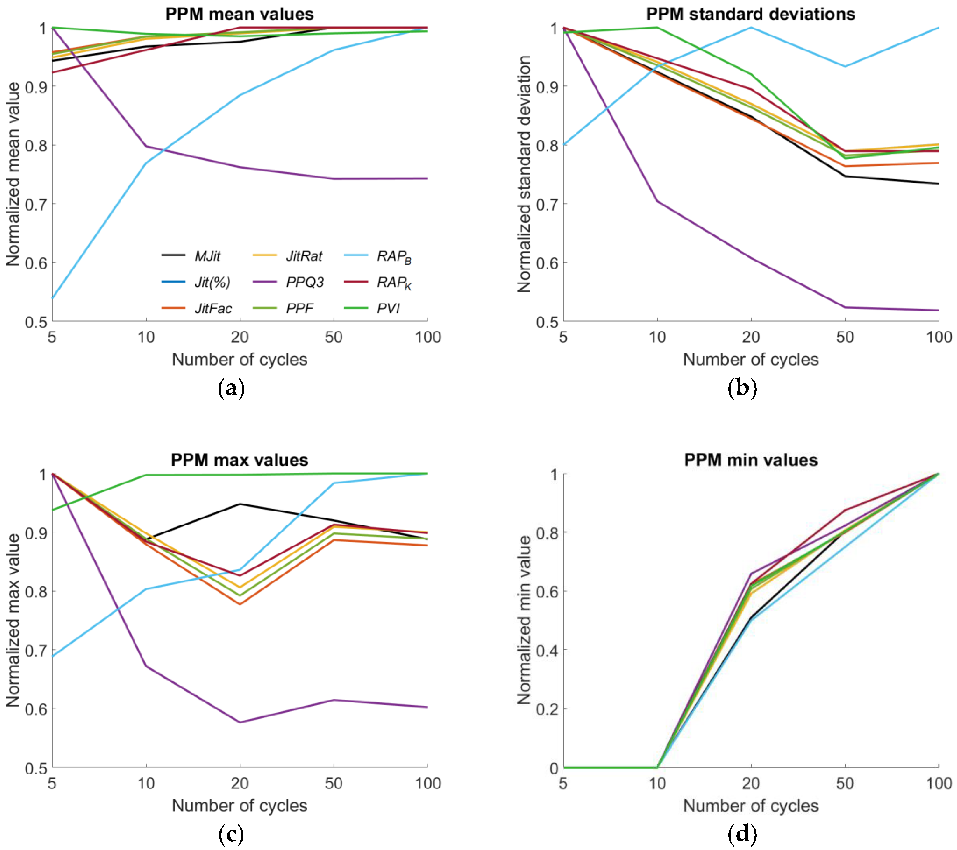
| Period Perturbation Measures (PPM) | ||||
| MJitC5 | 0.116 | 0.079 | 0.250 | 0.000 |
| MJitC10 | 0.119 | 0.073 | 0.222 | 0.000 |
| MJitC20 | 0.120 | 0.067 | 0.237 | 0.026 |
| MJitC50 | 0.123 | 0.059 | 0.230 | 0.041 |
| MJitC100 | 0.123 | 0.058 | 0.222 | 0.051 |
| Jit(%)C5 | 3.742 | 2.773 | 10.417 | 0.000 |
| Jit(%)C10 | 3.867 | 2.610 | 9.357 | 0.000 |
| Jit(%)C20 | 3.904 | 2.412 | 8.399 | 0.704 |
| Jit(%)C50 | 3.941 | 2.190 | 9.472 | 0.960 |
| Jit(%)C100 | 3.944 | 2.221 | 9.376 | 1.190 |
| JitFacC5 | 3.767 | 2.828 | 10.638 | 0.000 |
| JitFacC10 | 3.872 | 2.606 | 9.357 | 0.000 |
| JitFacC20 | 3.896 | 2.389 | 8.267 | 0.749 |
| JitFacC50 | 3.933 | 2.160 | 9.432 | 0.963 |
| JitFacC100 | 3.931 | 2.176 | 9.337 | 1.205 |
| JitRatC5 | 37.421 | 27.730 | 104.167 | 0.000 |
| JitRatC10 | 38.669 | 26.103 | 93.567 | 0.000 |
| JitRatC20 | 39.041 | 24.125 | 83.987 | 7.041 |
| JitRatC50 | 39.405 | 21.900 | 94.721 | 9.604 |
| JitRatC100 | 39.438 | 22.205 | 93.765 | 11.898 |
| PPQ3C5 | 3.566 | 2.893 | 10.468 | 0.000 |
| PPQ3C10 | 2.845 | 2.038 | 7.037 | 0.000 |
| PPQ3C20 | 2.718 | 1.758 | 6.034 | 0.535 |
| PPQ3C50 | 2.647 | 1.515 | 6.435 | 0.668 |
| PPQ3C100 | 2.649 | 1.501 | 6.307 | 0.812 |
| PPFC5 | 3.764 | 2.787 | 10.556 | 0.000 |
| PPFC10 | 3.881 | 2.608 | 9.383 | 0.000 |
| PPFC20 | 3.910 | 2.408 | 8.363 | 0.727 |
| PPFC50 | 3.942 | 2.180 | 9.478 | 0.962 |
| PPFC100 | 3.943 | 2.204 | 9.383 | 1.197 |
| RAPBC5 | 0.014 | 0.012 | 0.042 | 0.000 |
| RAPBC10 | 0.020 | 0.014 | 0.049 | 0.000 |
| RAPBC20 | 0.023 | 0.015 | 0.051 | 0.004 |
| RAPBC50 | 0.025 | 0.014 | 0.060 | 0.006 |
| RAPBC100 | 0.026 | 0.015 | 0.061 | 0.008 |
| RAPKC5 | 0.024 | 0.019 | 0.069 | 0.000 |
| RAPKC10 | 0.025 | 0.018 | 0.061 | 0.000 |
| RAPKC20 | 0.026 | 0.017 | 0.057 | 0.005 |
| RAPKC50 | 0.026 | 0.015 | 0.063 | 0.007 |
| RAPKC100 | 0.026 | 0.015 | 0.062 | 0.008 |
| PVIC5 | 1.193 | 0.782 | 2.604 | 0.000 |
| PVIC10 | 1.180 | 0.789 | 2.770 | 0.000 |
| PVIC20 | 1.175 | 0.726 | 2.771 | 0.213 |
| PVIC50 | 1.181 | 0.613 | 2.777 | 0.277 |
| PVIC100 | 1.185 | 0.628 | 2.777 | 0.345 |
| Parameter Name and Sequence Length | Average | Standard Deviation | Maximum | Minimum |
|---|---|---|---|---|
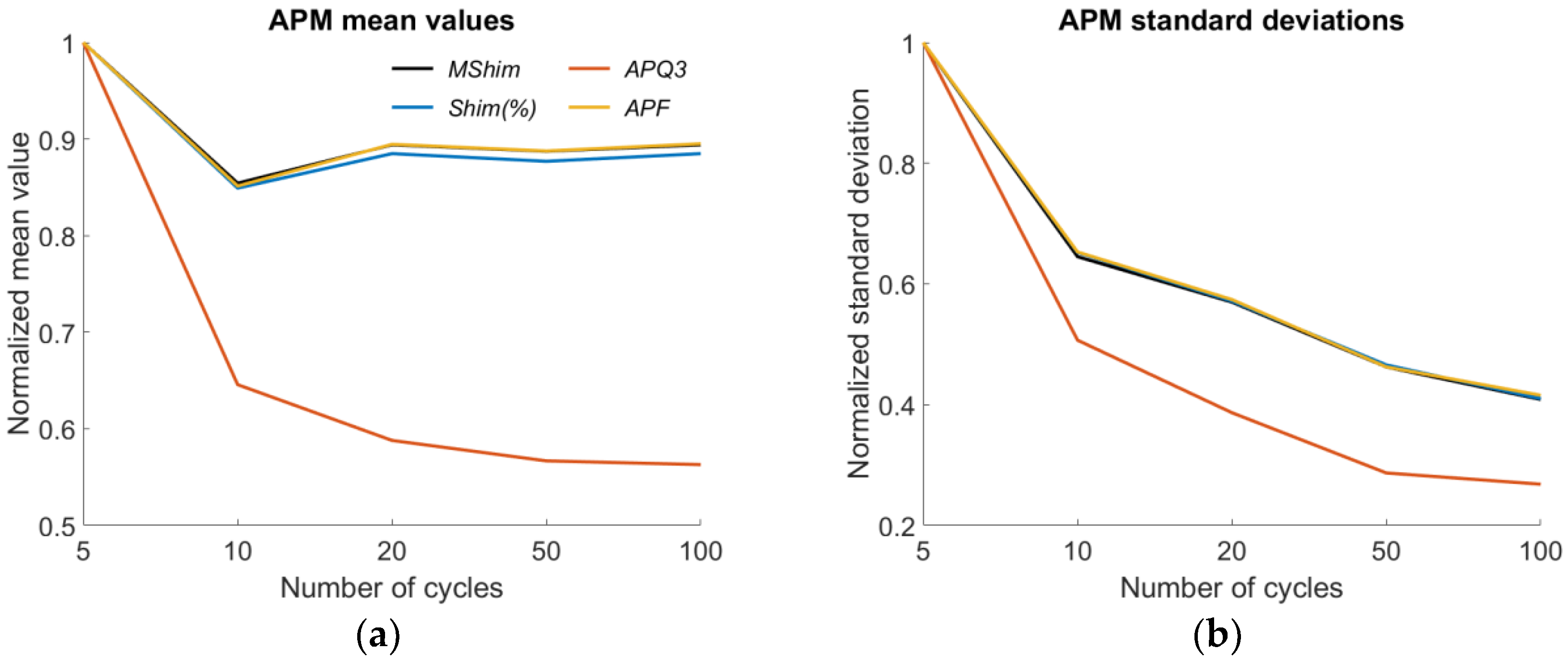
| Amplitude Perturbation Measures (APM) | ||||
| MShimC5 | 0.151 | 0.093 | 0.387 | 0.047 |
| MShimC10 | 0.129 | 0.060 | 0.301 | 0.061 |
| MShimC20 | 0.135 | 0.053 | 0.272 | 0.068 |
| MShimC50 | 0.134 | 0.043 | 0.247 | 0.064 |
| MShimC100 | 0.135 | 0.038 | 0.235 | 0.075 |
| Shim(%)C5 | 0.252 | 0.161 | 0.656 | 0.073 |
| Shim(%)C10 | 0.214 | 0.105 | 0.509 | 0.096 |
| Shim(%)C20 | 0.223 | 0.092 | 0.460 | 0.106 |
| Shim(%)C50 | 0.221 | 0.075 | 0.416 | 0.100 |
| Shim(%)C100 | 0.223 | 0.066 | 0.396 | 0.116 |
| APQ3C5 | 1.558 | 1.182 | 4.400 | 0.310 |
| APQ3C10 | 1.006 | 0.599 | 2.747 | 0.334 |
| APQ3C20 | 0.916 | 0.457 | 2.133 | 0.356 |
| APQ3C50 | 0.883 | 0.339 | 1.810 | 0.397 |
| APQ3C100 | 0.877 | 0.317 | 1.737 | 0.425 |
| APFC5 | 1.736 | 1.066 | 4.470 | 0.544 |
| APFC10 | 1.478 | 0.696 | 3.467 | 0.709 |
| APFC20 | 1.553 | 0.612 | 3.132 | 0.790 |
| APFC50 | 1.541 | 0.493 | 2.833 | 0.741 |
| APFC100 | 1.554 | 0.443 | 2.704 | 0.862 |
| AVIC5 | -0.907 | 0.366 | -0.273 | -1.530 |
| AVIC10 | -0.781 | 0.351 | -0.257 | -1.470 |
| AVIC20 | -0.493 | 0.316 | 0.283 | -1.078 |
| AVIC50 | -0.256 | 0.307 | 0.231 | -0.792 |
| AVIC100 | 0.015 | 0.379 | 0.910 | -0.630 |
| Parameter Name and Sequence Length | Average | Standard Deviation | Maximum | Minimum |
|---|---|---|---|---|
| Energy Perturbation Measures (EPM) | ||||
| EPQ3C5 | 9.880 | 7.443 | 23.847 | 0.499 |
| EPQ3C10 | 7.768 | 5.175 | 16.266 | 0.443 |
| EPQ3C20 | 7.395 | 4.466 | 14.732 | 1.777 |
| EPQ3C50 | 7.292 | 3.854 | 14.781 | 2.117 |
| EPQ3C100 | 7.295 | 3.701 | 14.341 | 2.528 |
| EPFC5 | 11.089 | 6.934 | 24.424 | 0.869 |
| EPFC10 | 11.108 | 6.517 | 21.952 | 1.209 |
| EPFC20 | 11.233 | 6.209 | 20.983 | 2.812 |
| EPFC50 | 11.384 | 5.526 | 22.090 | 3.340 |
| EPFC100 | 11.392 | 5.381 | 21.629 | 4.210 |
References
- Titze, I.R. Principles of Voice Production, 2nd ed.; National Center for Voice and Speech: Iowa City, IA, USA, 2000; pp. 87–183. [Google Scholar]
- Stevens, K.N. Source Mechanisms. In Acoustic Phonetics; Keyser, S.J., Ed.; MIT Press: Cambridge, MA, USA, 2000; pp. 55–126. [Google Scholar]
- Baken, R.J.; Orlikoff, R.F. Vocal fundamental frequency. In Clinical Measurement of Speech & Voice, 2nd ed.; Cengage Learning: Clifton Park, NY, USA, 1999. [Google Scholar]
- Kendall, K.A. Clinical Applications for High-Speed Laryngeal Imaging. In Laryngeal Evaluation; Kendall, K., Leonard, R., Eds.; Georg Thieme: New York City, NY, USA, 2010; p. 272. [Google Scholar]
- Švec, J.G.; Schutte, H.K. Videokymography: High-speed line scanning of vocal fold vibration. J. Voice 1996, 10, 201–205. [Google Scholar] [CrossRef]
- Echternach, M.; Döllinger, M.; Sundberg, J.; Traser, L.; Richter, B. Vocal fold vibrations at high soprano fundamental frequencies. J. Acoust. Soc. Am. 2013, 133, 82–87. [Google Scholar] [CrossRef] [PubMed]
- Deliyski, D. Laryngeal High-Speed Videoendoscopy. In Laryngeal Evaluation; Kendall, K., Leonard, R., Eds.; Georg Thieme: New York City, NY, USA, 2010; pp. 245–270. [Google Scholar]
- Phadke, K.V.; Vydrová, J.; Domagalská, R.; Švec, J.G. Evaluation of clinical value of videokymography for diagnosis and treatment of voice disorders. Eur. Arch. Otorhinolaryngol. 2017, 274, 3941–3949. [Google Scholar] [CrossRef] [PubMed]
- Švec, J.G.; Sundberg, J.; Hertegård, S. Three registers in an untrained female singer analyzed by videokymography, strobolaryngoscopy and sound spectrography. J. Acoust. Soc. Am. 2008, 123. [Google Scholar] [CrossRef] [PubMed]
- Dejonckere, P.H.; Lebacq, J.; Bocchi, L.; Orlandi, S.; Manfredi, C. High-speed single line scan: An application in singing pedagogy. Ephonoscope 2016, 2, 273–286. [Google Scholar]
- Deliyski, D.; Hillman, R. State of the art laryngeal imaging: Research and clinical implications. Curr. Opin. Otolaryngol. Head Neck Surg. 2010, 18, 147–152. [Google Scholar] [CrossRef] [PubMed]
- Patel, R.R.; Dubrovskiy, D.; Döllinger, M. Measurement of glottal cycle characteristics between children and adults: Physiological variations. J. Voice 2014, 28, 476–486. [Google Scholar] [CrossRef] [PubMed]
- Poburka, B.J.; Patel, R.R.; Bless, D.M. Voice-vibratory assessment with laryngeal imaging (VALI) form: Reliability of rating stroboscopy and high-speed videoendoscopy. J. Voice 2017, 31, 513.e1–513.e14. [Google Scholar] [CrossRef] [PubMed]
- Zacharias, S.R.C.; Myer, C.M.; Meinzen-Derr, J.; Kelchner, L.; Deliyski, D.D.; Alarcón, A. Comparison of videostroboscopy and high-speed videoendoscopy in evaluation of supraglottic phonation. Ann. Otol. Rhinol. Laryngol. 2016, 125, 829–837. [Google Scholar] [CrossRef] [PubMed]
- Döllinger, M.; Lohscheller, J.; McWhorter, A.; Kunduk, M. Variability of normal vocal fold dynamics for different vocal loading in one healthy subject investigated by phonovibrograms. J. Voice 2009, 23, 175–181. [Google Scholar] [CrossRef] [PubMed]
- Semmler, M.; Kniesburges, S.; Parchent, J.; Jakubaß, B.; Zimmermann, M.; Bohr, C.; Schützenberger, A.; Döllinger, M. Endoscopic laser-based 3D imaging for functional voice diagnostics. Appl. Sci. 2017, 7. [Google Scholar] [CrossRef]
- Deliyski, D.D.; Petrushev, P.P.; Bonilha, H.S.; Gerlach, T.T.; Martin-Harris, B.; Hillman, R.E. Clinical implementation of laryngeal high-speed videoendoscopy: Challenges and evolution. Folia Phoniatrica et Logopaedica 2007, 60, 33–44. [Google Scholar] [CrossRef] [PubMed]
- Mehta, D.D.; Zañartu, M.; Quatieri, T.F.; Deliyski, D.D.; Hillman, R.E. Investigating acoustic correlates of human vocal fold vibratory phase asymmetry through modeling and laryngeal high-speed videoendoscopy. J. Acoust. Soc. Am. 2011, 130. [Google Scholar] [CrossRef] [PubMed]
- Ishikawa, C.C.; Pinheiro, T.G.; Hachiya, A.; Montagnoli, A.N.; Tsuji, D.H. Impact of cricothyroid muscle contraction on vocal fold vibration: Experimental study with high-speed videoendoscopy. J. Voice 2017, 31, 300–306. [Google Scholar] [CrossRef] [PubMed]
- Stellan, H. What have we learned about laryngeal physiology from high-speed digital videoendoscopy? Curr. Opin. Otolaryngol. Head Neck Surg. 2005, 13, 152–156. [Google Scholar] [CrossRef]
- Rasp, O.; Lohscheller, J.; Döllinger, M.; Eysholdt, U.; Hoppe, U. The pitch rise paradigm: A new task for real-time endoscopy of non-stationary phonation. Folia Phoniatrica et Logopaedica 2006, 58, 175–185. [Google Scholar] [CrossRef] [PubMed]
- Zacharias, S.R.C.; Deliyski, D.D.; Gerlach, T.T. Utility of laryngeal high-speed videoendoscopy in clinical voice assessment. J. Voice 2018, 32, 216–220. [Google Scholar] [CrossRef] [PubMed]
- Patel, R.; Dailey, S.; Bless, D. Comparison of high-speed digital imaging with stroboscopy for laryngeal imaging of glottal disorders. Ann. Otol. Rhinol. Laryngol. 2008, 117, 413–424. [Google Scholar] [CrossRef] [PubMed]
- Hartnick, C.J.; Zeitels, S.M. Pediatric video laryngo-stroboscopy. Int. J. Pediatr. Otorhinolaryngol. 2005, 69, 215–219. [Google Scholar] [CrossRef] [PubMed]
- Vaca, M.; Cobeta, I.; Mora, E.; Reyes, P. Clinical assessment of glottal insufficiency in age-related dysphonia. J. Voice 2017, 31, 128.e1–128.e5. [Google Scholar] [CrossRef] [PubMed]
- Stemple, J.C.; Fry, L.B. Performing Videostroboscopy. In Laryngeal Evaluation; Kendall, K., Leonard, R., Eds.; Georg Thieme: New York City, NY, USA, 2010; p. 110. [Google Scholar]
- Wendler, J.; Seidner, W.; Eysholdt, U. Lehrbuch der Phoniatrie und Pädaudiologie, 4th ed.; Thieme: Stuttgart, Germany, 2005; pp. 113–120. [Google Scholar]
- Noordzij, P.J.; Woo, P. Glottal Area Waveform Analysis of Benign Vocal Fold Lesions before and after Surgery. Ann. Otol. Rhinol. Laryngol. 2000, 109, 441–446. [Google Scholar] [CrossRef] [PubMed]
- Mendez, A.; Gracia, B.; Ruiz, I.; Iturricha, I. Glottal Area Segmentation without Initialization using Gabor Filters. In Proceedings of the IEEE International Symposium on Signal Processing and Information Technology (ISSPIT), Sarajevo, Bosnia and Herzegovina, 16–19 December 2008. [Google Scholar] [CrossRef]
- Kunduk, M.; Yan, Y.; McWhorther, A.J.; Bless, D. Investigation of voice initiation and voice offset characteristics with high-speed digital imaging. Logop. Phoniatr. Vocol. 2006, 31, 139–144. [Google Scholar] [CrossRef] [PubMed]
- Chen, X.; Bless, D.; Yan, Y. A Segmentation Scheme Based on Rayleigh Distribution Model for Extracting Glottal Waveform from High-speed Laryngeal Images. In Proceedings of the 27th Annual International Conference of the Engineering in Medicine and Biology Society (IEEE-EMBS), Shanghai, China, 17–18 January 2006. [Google Scholar] [CrossRef]
- Patel, R.R.; Unnikrishnan, H.; Donohue, K.D. Effects of vocal fold nodules on glottal cycle measurements derived from high-speed videoendoscopy in children. PLoS ONE 2016, 11. [Google Scholar] [CrossRef] [PubMed]
- Petermann, S.; Döllinger, M.; Kniesburges, S.; Ziethe, A. Analysis method for the neurological and physiological processes underlying the pitch-shift reflex. Acta Acust. United Acust. 2016, 102, 284–297. [Google Scholar] [CrossRef]
- Deliyski, D.D.; Shaw, H.S.; Evans, M.K. Influence of sampling rate on accuracy and reliability of acoustic voice analysis. Logop. Phoniatr. Vocol. 2005, 30, 55–62. [Google Scholar] [CrossRef] [PubMed]
- Schützenberger, A.; Kunduk, M.; Döllinger, M.; Alexiou, C.; Dubrovskiy, D.; Semmler, M.; Seger, A.; Bohr, C. Laryngeal high-speed videoendoscopy: Sensitivity of objective parameters towards recording frame rate. BioMed Res. Int. 2016, 2016. [Google Scholar] [CrossRef] [PubMed]
- Scherer, R.; Vail, V.; Guo, C. Required number of tokens to establish reliable voice perturbation values. NCVS Status Prog. Rep. 1994, 7, 107–117. [Google Scholar]
- Karnell, M.P.; Hall, K.D.; Landahl, K.L. Comparison of fundamental frequency and perturbation measurements among three analysis systems. J. Voice 1995, 9, 383–393. [Google Scholar] [CrossRef]
- Hohm, J.; Döllinger, M.; Bohr, C.; Kniesburges, S.; Ziethe, A. Influence of F_0 and sequence length of audio and electroglottographic signals on perturbation measures for voice assessment. J. Voice 2015, 29, 517.e11–517.e21. [Google Scholar] [CrossRef] [PubMed]
- Bohr, C.; Kraeck, A.; Eysholdt, U.; Ziethe, A.; Döllinger, M. Quantitative analysis of organic vocal fold pathologies in females by high-speed endoscopy. Laryngoscope 2013, 123, 1686–1693. [Google Scholar] [CrossRef] [PubMed]
- Patel, R.R.; Walker, R.; Sivasankar, P.M. Spatiotemporal quantification of vocal fold vibration after exposure to superficial laryngeal dehydration: A preliminary study. J. Voice 2016, 30, 427–433. [Google Scholar] [CrossRef] [PubMed]
- Vlot, C.; Ogawa, M.; Hosokawa, K.; Iwahashi, T.; Kato, C.; Inohara, H. Investigation of the immediate effects of humming on vocal fold vibration irregularity using electroglottography and high-speed laryngoscopy in patients with organic voice disorders. J. Voice 2017, 31, 48–56. [Google Scholar] [CrossRef] [PubMed]
- Arbeiter, M.; Petermann, S.; Hoppe, U.; Bohr, C.; Döllinger, M.; Ziethe, A. Analysis of the auditory feedback and phonation in normal voices. Ann. Otol. Rhinol. Laryngol. 2017, 127, 89–98. [Google Scholar] [CrossRef] [PubMed]
- Krausert, C.R.; Liang, Y.; Zhang, Y.; Rieves, A.L.; Geurink, K.R.; Jiang, J.J. Spatiotemporal analysis of normal and pathological human vocal fold vibrations. Am. J. Otolaryngol. 2012, 33, 641–649. [Google Scholar] [CrossRef] [PubMed]
- Horii, Y. Vocal shimmer in sustained phonation. J. Speech Lang. Hear. Res. 1980, 23, 202–209. [Google Scholar] [CrossRef]
- Hollien, H.; Michel, J.; Doherty, T.E. A method for analyzing vocal jitter in sustained phonation. J. Phon. 1973, 1, 85–91. [Google Scholar]
- Horii, Y. Fundamental frequency perturbation observed in sustained phonation. J. Speech Lang. Hear. Res. 1979, 22, 5–19. [Google Scholar] [CrossRef]
- Kasuya, H.; Endo, Y.; Saliu, S. Novel acoustic measurements of jitter and shimmer characteristics from pathological voice. In Proceedings of the EUROSPEECH’93, Berlin, Germany, 22–25 September 1993; pp. 1973–1976. [Google Scholar]
- Bielamowicz, S.; Kreiman, J.; Gerratt, B.; Dauer, M.; Berke, G. Comparison of voice analysis systems for perturbation measurement. J. Speech Hear. Res. 1996, 39, 126–134. [Google Scholar] [CrossRef] [PubMed]
- Koike, Y. Application of some acoustic measures for the evaluation of laryngeal dysfunction. Stud. Phonol. 1973, 7, 17–23. [Google Scholar] [CrossRef]
- Deal, R.E.; Emanuel, F.W. Some waveform and spectral features of vowel roughness. J. Speech Lang. Hear. Res. 1978, 21, 250–264. [Google Scholar] [CrossRef]
- Schlegel, P.; Stingl, M.; Kunduk, M.; Kniesburges, S.; Bohr, C.; Döllinger, M. Dependencies and ill-designed parameters within high-speed videoendoscopy and acoustic signal analysis. J. Voice 2018. [Google Scholar] [CrossRef] [PubMed]
- Lohscheller, J.; Döllinger, M.; Schuster, M.; Eysholdt, U.; Hoppe, U. The laryngectomee substitute voice: Image processing of endoscopic recordings by fusion with acoustic signals. Methods Inf. Med. 2003, 42, 277–281. [Google Scholar] [CrossRef] [PubMed]


| Parameter (Unit) and Reference | Abbreviation | Parameter Description |
|---|---|---|
| Period Perturbation Measures (PPM) | ||
| Mean Jitter (ms) [44] | MJit | Mean deviation in duration between cycle pairs |
| Jitter (%) (a.u.) [44] | Jit(%) | Normalized mean deviation in duration between cycle pairs |
| Jitter Factor (a.u.) [45] | JitFac | Normalized mean deviation of reciprocal in duration between cycle pairs |
| Jitter Ratio (a.u.) [46] | JitRat | Normalized mean deviation in duration between cycle pairs |
| Period Perturbation Quotient-3% (a.u.) [47] 1 | PPQ3 | Difference in cycle lengths based on the mean difference between each inner cycle and its neighboring cycles |
| Period Perturbation Factor (a.u.) [47] 1 | PPF | Mean normalized deviation in duration between cycle pairs |
| Relative Average Perturbation Bielamowicz (a.u.) [48] | RAPB | Difference in cycle lengths based on the difference between each inner cycle and its neighboring cycles |
| Relative Average Perturbation Koike (a.u.) [49] | RAPK | Normalized difference in cycle lengths based on the difference between each inner cycle and its neighboring cycles |
| Period Variability Index (a.u.) [50] | PVI | Normalized mean quadratic deviation in duration between each cycle and an average cycle |
| Amplitude Perturbation Measures (APM) | ||
| Mean Shimmer (decibel) [44] | MShim | Mean logarithmized deviation in dynamic range 2 between cycle pairs |
| Shimmer (%) (dB/log10(pixel)) [51] | Shim(%) | Normalized mean logarithmized deviation in dynamic range between cycle pairs |
| Amplitude Perturbation Quotient-3% (a.u.) [47] | APQ3 | Difference in dynamic range based on the mean difference between each inner cycle and its neighboring cycles |
| Amplitude Perturbation Factor (a.u.) [47] | APF | Mean normalized deviation in dynamic range between cycle pairs |
| Amplitude Variability Index (decibel) [50] | AVI | Logarithmized normalized mean quadratic deviation in dynamic range between each cycle and an average cycle |
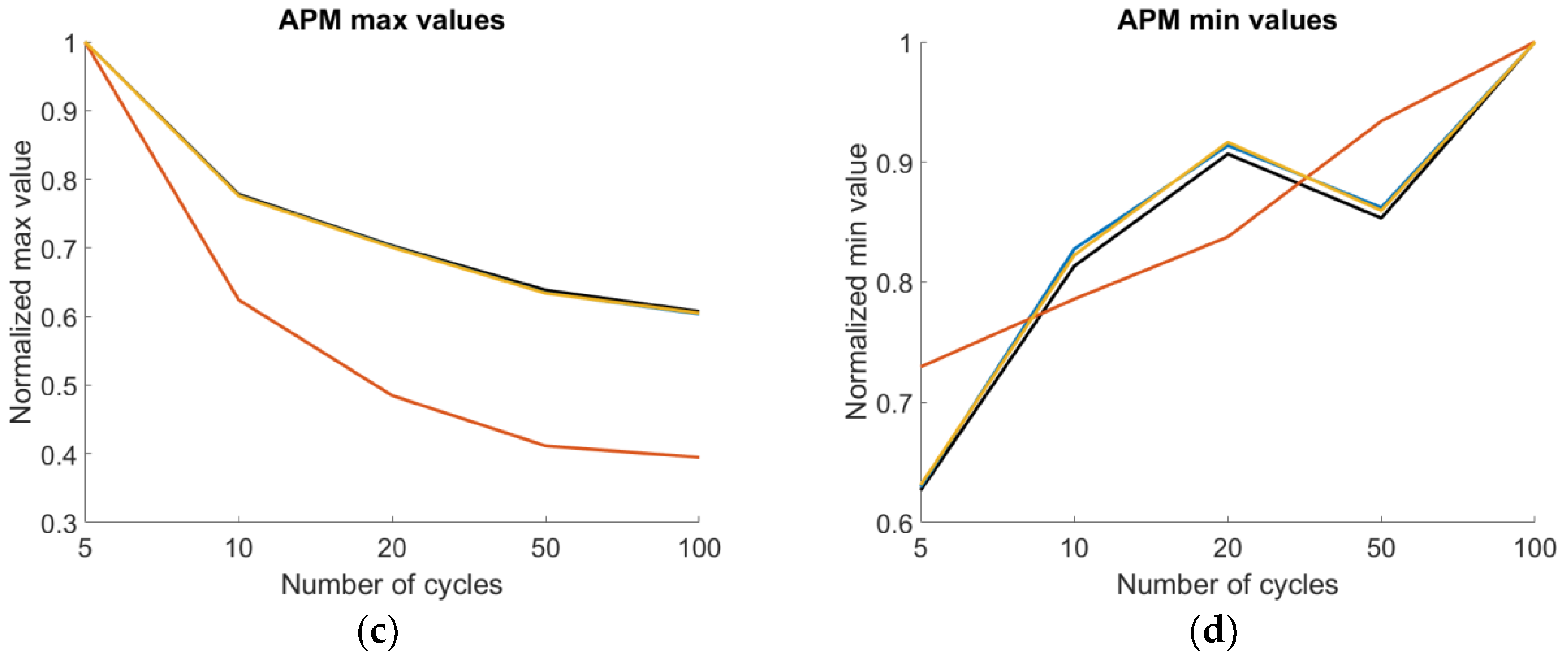
| Energy Perturbation Measures (EPM) | ||
| Energy Perturbation Quotient-3% (a.u.) [47] | EPQ3 | Difference in energy based on the mean difference between each inner cycle and its neighboring cycles |
| Energy Perturbation Factor (a.u.) [47] | EPF | Mean normalized deviation in energy between cycle pairs |
| Statistically Significant Changes | ||||
| Parameter | Overall Test Significance | Significantly Different Cycle Pairings | ||
| RAPB | p < 0.001 | 5–10, 5–20, 5–50, 5–100, 10–20 | ||
| APQ3 | p = 0.017 | 5–10, 5–20, 5–50 | ||
| AVI | p < 0.001 | 5–20, 5–50, 5-100, 10–50, 10–100, 20–50, 20–100, 50–100 | ||
| Systematic in- or decreases | ||||
| Parameter | Mean value | Standard deviation | Max value | Min value |
| Period Perturbation Measures (PPM) | ||||
| MJit | ➚50 1 | ➘100 2 | ➘10 | ➚100 |
| Jit(%) | ➚100 | ➘50 | ➘20 | ➚100 |
| JitFac | ➚50 | ➘50 | ➘20 | ➚100 |
| JitRat | ➚100 | ➘50 | ➘20 | ➚100 |
| PPQ3 | ➘50 | ➘100 | ➘20 | ➚100 |
| PPF | ➚100 | ➘50 | ➘20 | ➚100 |
| RAPB | ➚100 | ➚20 | ➚100 | ➚100 |
| RAPK | ➚100 | ➘50 | ➘20 | ➚100 |
| PVI | ➘20 | ➚10 | ➚100 | ➚100 |
| Amplitude Perturbation Measures (APM) | ||||
| MShim | ➘10 | ➘100 | ➘100 | ➚20 |
| Shim(%) | ➘10 | ➘100 | ➘100 | ➚20 |
| APQ3 | ➘100 | ➘100 | ➘100 | ➚100 |
| APF | ➘10 | ➘100 | ➘100 | ➚20 |
| AVI | ➚100 | ➘50 | ➚20 | ➚100 |
| Energy Perturbation Measures (EPM) | ||||
| EPQ3 | ➘50 | ➘100 | ➘20 | ➘10 |
| EPF | ➚100 | ➘100 | ➘20 | ➚100 |
© 2018 by the authors. Licensee MDPI, Basel, Switzerland. This article is an open access article distributed under the terms and conditions of the Creative Commons Attribution (CC BY) license (http://creativecommons.org/licenses/by/4.0/).
Share and Cite
Schlegel, P.; Semmler, M.; Kunduk, M.; Döllinger, M.; Bohr, C.; Schützenberger, A. Influence of Analyzed Sequence Length on Parameters in Laryngeal High-Speed Videoendoscopy. Appl. Sci. 2018, 8, 2666. https://doi.org/10.3390/app8122666
Schlegel P, Semmler M, Kunduk M, Döllinger M, Bohr C, Schützenberger A. Influence of Analyzed Sequence Length on Parameters in Laryngeal High-Speed Videoendoscopy. Applied Sciences. 2018; 8(12):2666. https://doi.org/10.3390/app8122666
Chicago/Turabian StyleSchlegel, Patrick, Marion Semmler, Melda Kunduk, Michael Döllinger, Christopher Bohr, and Anne Schützenberger. 2018. "Influence of Analyzed Sequence Length on Parameters in Laryngeal High-Speed Videoendoscopy" Applied Sciences 8, no. 12: 2666. https://doi.org/10.3390/app8122666
APA StyleSchlegel, P., Semmler, M., Kunduk, M., Döllinger, M., Bohr, C., & Schützenberger, A. (2018). Influence of Analyzed Sequence Length on Parameters in Laryngeal High-Speed Videoendoscopy. Applied Sciences, 8(12), 2666. https://doi.org/10.3390/app8122666