1. Introduction
Throughout the last 50 years, chaotic dynamical systems have attracted increasing attention due to their applicability in a range of diverse and multidisciplinary fields. A dynamical system is said to be chaotic if its states are extremely sensitive to small variations in the initial conditions. Another important property of chaotic systems is that they have attractors characterized by a complicated set of points with a fractal structure commonly referred to as a strange attractor. This chaotic behavior was first observed in continuous dynamical systems and was thought to be an undesirable property. The first chaotic system encountered in the modeling of a real-life phenomena is that of Lorenz [
1], which describes atmospheric convection. Soon after, researchers found that chaotic systems can also be discrete. A number of chaotic maps were proposed throughout the years including the Hénon map [
2], the logistic map [
3], the Lozi map [
4], the 3D Stefanski map [
5], the Rössler map [
6], and many more. Recently, nonlinear oscillations on Riemannian manifolds that can exhibit a chaotic behavior were introduced in [
7,
8]. Other related works include an investigation of the chaotic dynamics in a fractional love model with an external environment, as in [
9], and an extension using a fuzzy function [
10].
In recent years, with the growing interest in fractional discrete calculus [
11], people have started looking into fractional chaotic maps. Although fractional maps come with considerable added complexity, they provide better flexibility in the modeling of natural phenomena and lead to richer dynamics with more degrees of freedom. Among the fractional chaotic maps that have been proposed, studied, and applied over the last five years are the fractional logistic map [
12], the fractional Hénon map [
13], the generalized hyperchaotic Hénon map [
14], and the fractional unified map [
15]. Perhaps the main concern of the research community has been the possibility of controlling and synchronizing these types of maps [
15,
16,
17,
18,
19,
20]. An application of a generalized fractional logistic map to data encryption and its FPGA implementation was achieved in [
21].
In this paper, we are interested in the Tinkerbell discrete-time chaotic system, which is of the form:
where
,
,
, and
are system parameters and
n represents the discrete iteration step. It is rumored that the map (
1) derives its name from the famous Cinderella story, as the trajectory followed by the map resembles that of Tinkerbell appearing in the movie adaptation of the fairy tale. The Tinkerbell map has been studied by many as it exhibits very rich dynamics including a chaotic behavior and a range of periodic states. For instance, its bifurcation subject to different scenarios and initial settings has been studied in [
22,
23,
24,
25]. A more comprehensive study was performed in [
26]. The authors identified conditions for the existence of fold bifurcation, flip bifurcation, and Hopf bifurcation in the Tinkerbell map.
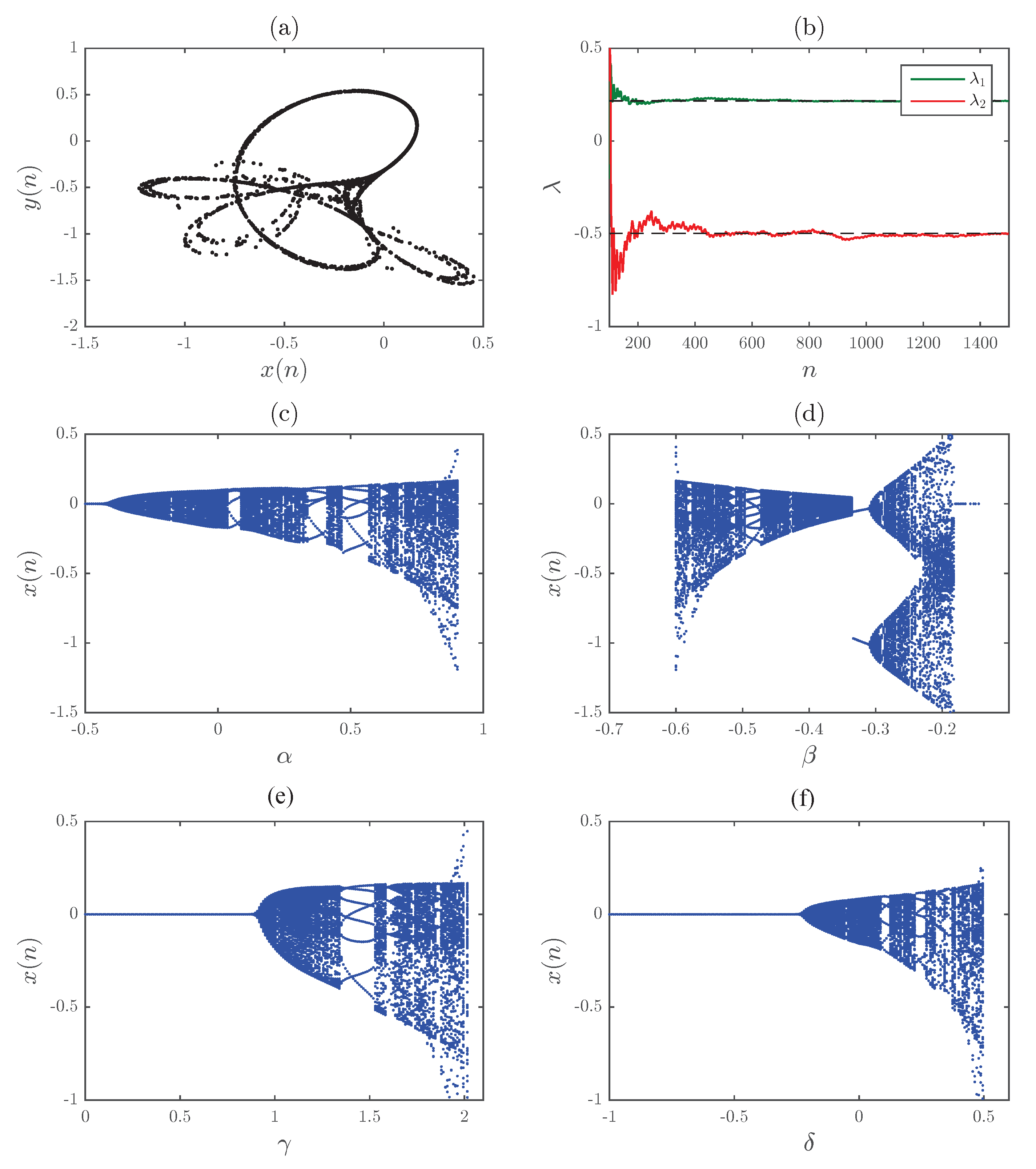
In order to visualize the dynamics of the map (
1), we resort to phase plots, bifurcation diagrams, and Lyapunov exponent estimation. We assume parameter values
,
,
, and
and initial states
. The results are depicted in
Figure 1. The Tinkerbell map’s phase plot is depicted in
Figure 1a. Based on
Figure 1b, we can see that the estimated Lyapunov exponents of (
1) are given by
and
. It is well known that a positive Lyapunov exponent indicates a chaotic behavior. The remaining parts of
Figure 1 depict the bifurcation diagrams of the map (
1) with respect to different parameters. These diagrams confirm that the map exhibits a range of different behaviors.
It should be clear to the reader that the Tinkerbell map has rich dynamics and is heavily dependent on its parameters, as well as the initial setting. The main objective of this paper is to investigate the fractional Caputo-difference form of the Tinkerbell map in order to benefit from the added degrees of freedom due to the fractional nature. It is expected that the fractional form will have even richer dynamics and may consequently be more suitable for applications that require a higher entropy level such as data/image encryption.
2. Fractional Tinkerbell Map
In this section, we use recent developments in fractional discrete calculus to define the Caputo-difference fractional map corresponding to (
1). First, let us define the
fractional sum of anarbitrary function
[
27] as:
for
and
, where
. Note that the term
is known as the falling function and may be defined by means of the Gamma function
as:
Based on this definition of the fractional sum, we may define the Caputo-like fractional difference operator.
In this section, we would like to produce a fractional difference form of the Tinkerbell map (
1). First, we take the difference form, which for function
with fractional order
is given by:
Substituting yields the final form proposed in [
28], which is defined as:
where
and
.
We are now ready to examine the fractional map. First, we take the difference form of (
1) to obtain:
We may replace the standard difference in (
6) with the Caputo-difference, which yields:
for
,
,
a is the starting point, and
is a Caputo-like difference operator. The case
corresponds to the non-fractional scenario (
1).
3. Dynamics of the Fractional Tinkerbell Map
In this section, we will employ numerical tools to assess the dynamics of the proposed fractional Tinkerbell map (
7). For that, we will need a discrete numerical formula that allows us to evaluate the states of the map in fractional discrete time. According to [
29] and other similar studies, we can evaluate (
7) numerically as:
where we assumed
for simplicity. This yields an initial-value problem similar to that of [
30], which allows us to use a similar discrete integral equation.
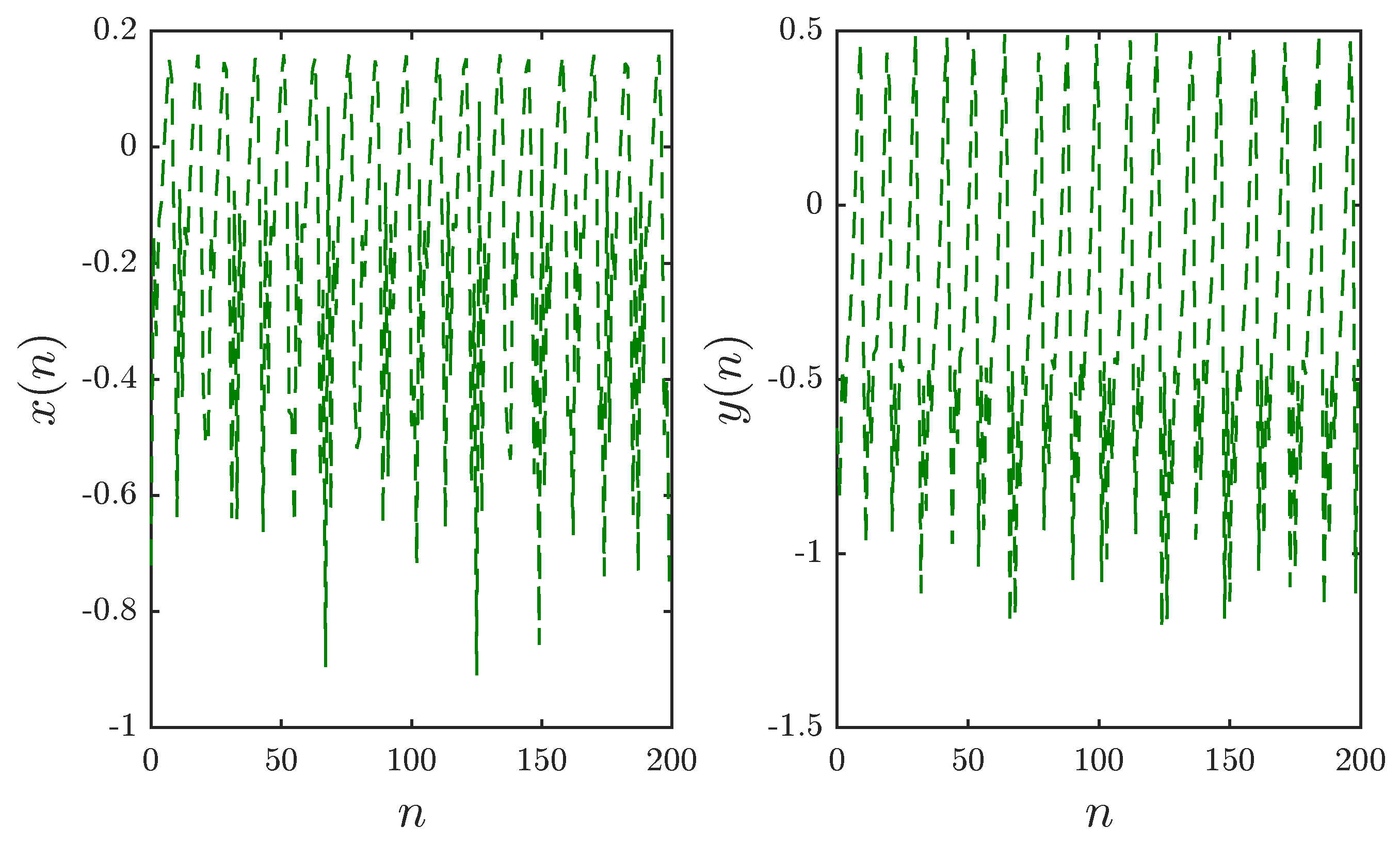
Using Formula (
8), we may obtain the states of the fractional Tinkerbell map and consequently produce time series plots of the states, phase-space plots, and bifurcation diagrams. We start with a simple case where the parameters and initial conditions are identical to those adopted in the standard case, i.e.,
and
. Given the fractional order
,
Figure 2 depicts the discrete time evolution of the states. Since the time series in
Figure 2 do not indicate the existence or absence of chaos definitively, it is more convenient to show the trajectories followed by the map in state space.
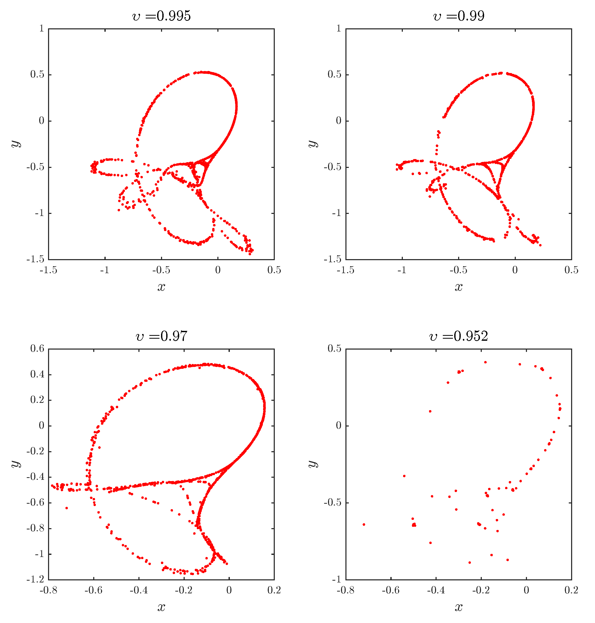
Figure 3 shows the phase plots for different values of the fractional order
. We see that the overall Tinkerbell shape remains valid for a short range of fractional orders. As the order gets close to
, the trajectory almost completely disappears.
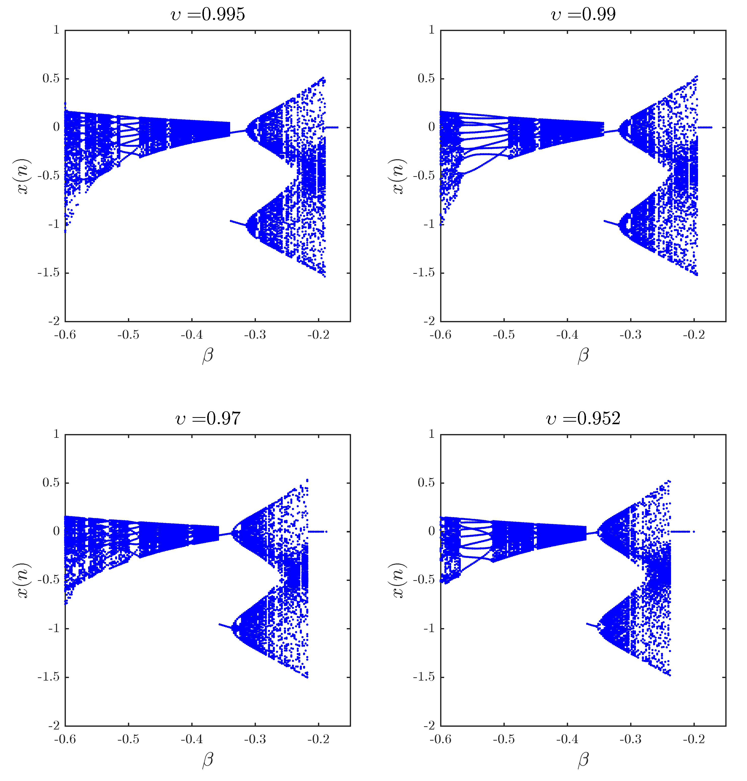
Although the phase plots give an indication of the behavior of the map, it is not until we visualize the bifurcation of the map subject to different parameters that a more complete picture forms. We choose the parameter
as the critical parameter and varied it over the range
in steps of
. The process may be easily repeated for other parameters. The bifurcation diagrams obtained using the same parameter and initial condition values from earlier are depicted in
Figure 4. We observe that although the general dynamics remain similar, the intervals seem to become shorter as the fractional order is decreased.
Even though these bifurcation diagrams suggest the existence of chaos in the fractional Tinkerbell map, they are not definitive. Generally, in order to prove the existence of chaos, we must use multiple tools including time series, phase portraits, Poincaré maps, power spectra, bifurcation diagrams, Lyapunov exponents, etc. The next tool at our disposal is Lyapunov exponents. We calculate these exponents by means of the Jacobian method. It is well known that when
is positive and the points in the corresponding bifurcation diagram are dense, the map is highly likely to be chaotic.
Figure 5 shows the largest Lyapunov exponents corresponding to the same bifurcation diagrams depicted in
Figure 4 in the
x-
plane. We can observe clearly that for certain ranges of the parameter
, chaos exists.
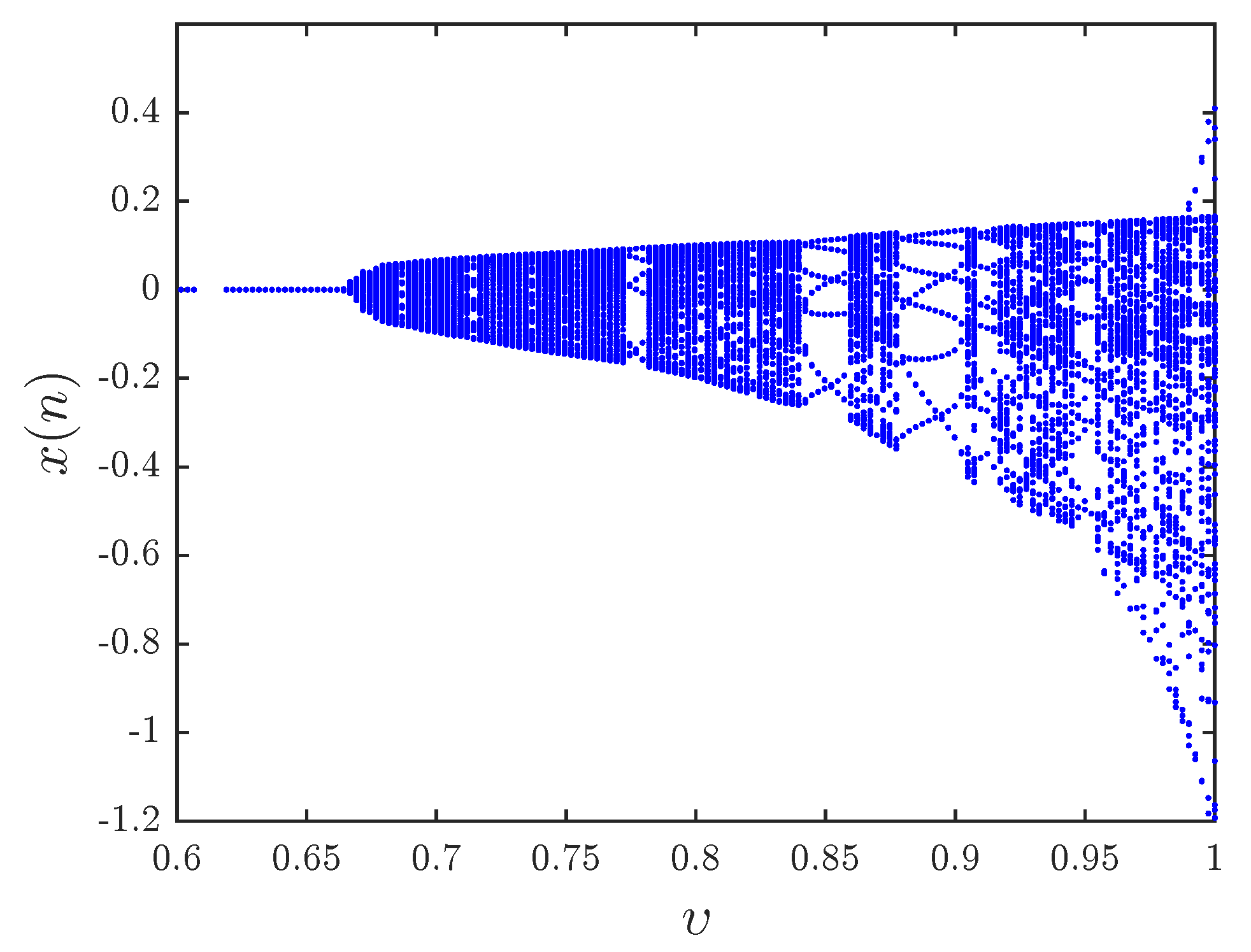
Another interesting aspect is the effect of the fractional order on the dynamics of the map for a specific set of parameter values. We fix the parameters and initial conditions at
and
, respectively.
Figure 6 shows the bifurcation plot with the critical parameter
being changed in steps of
. This is interesting in that it shows that although the chaotic behavior disappears when the fractional order drops close to
, it is observed again over intermittent intervals. Chaos does not disappear totally until the fractional order is very low.
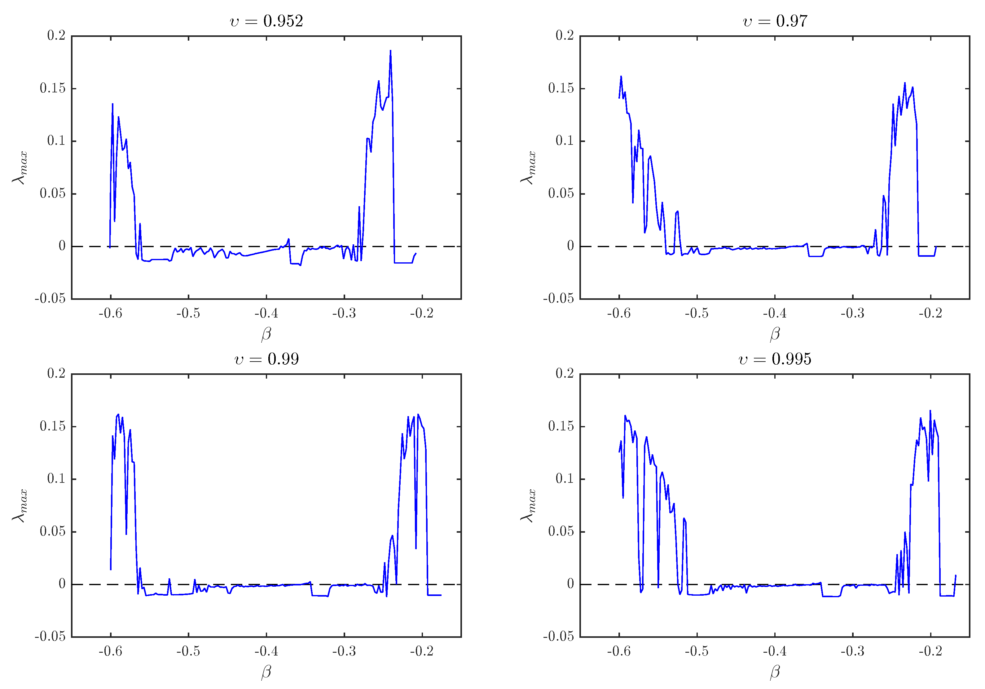
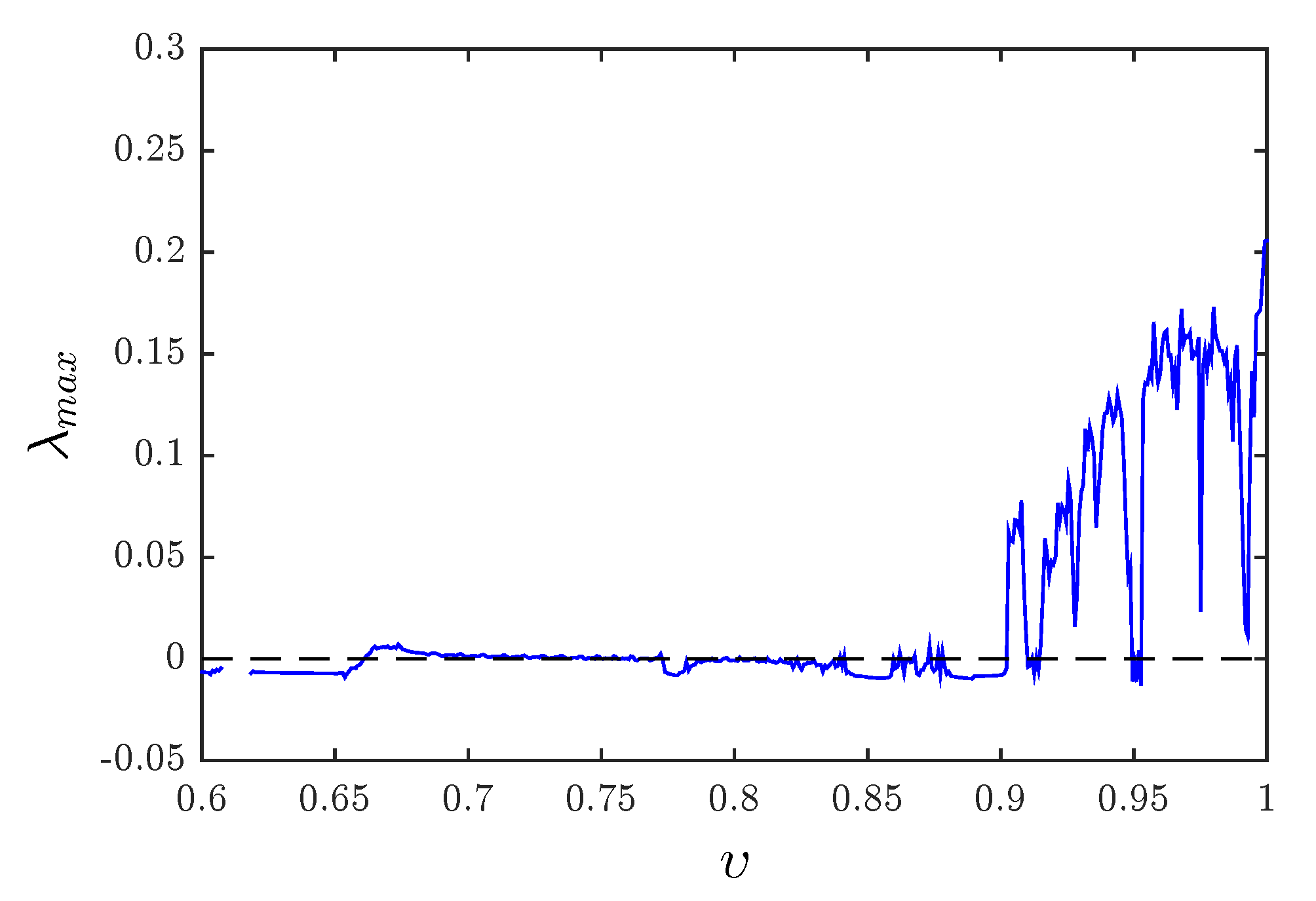
The largest Lyapunov exponent corresponding to the this bifurcation diagram in the
x-
plane is depicted in
Figure 7. From the figure, we observe that for a fractional order larger than 0.952,
is positive, which implies that the fractional Tinkerbell map is chaotic. During the interval
,
is observed to change intermittently between positive and negative signs, which means that chaos starts to appear and disappear. Finally, for values lower than
, chaos disappears completely. These results agree with the bifurcation diagram in
Figure 6.
4. Control of the Fractional Tinkerbell Map
In this section, we show that the proposed fractional Tinkerbell can be stabilized by means of a simple adaptive feedback controller. In order to be able to establish the asymptotic convergence of the controlled states towards zero, we first need to recall some important results from the literature concerning the asymptotic stability of fractional discrete systems. Since fractional discrete calculus is still relatively new, the existing literature related to stability is very limited. There are two main ways of establishing asymptotic stability. The first relies on the linearity of the system and places conditions on the eigenvalues of the Jacobian [
31]. The second scheme is a generalization of the well-known Lyapunov direct method [
32]. Although, the Lyapunov method is powerful and can support different types of systems, its has yet to be established for delayed fractional discrete systems, which renders it unusable for the system at hand. Hence, our objective here is to design the control laws to linearize the system, which will allow us to use the stability theory of linear systems. The following theorem summarizes the result of [
31].
Theorem 1. The zero equilibrium of the linear fractional discrete system:where , , and , is asymptotically stable if the eigenvalues λ of M satisfy:for all . Consider the controlled version of (
7) given by:
where
and
are adaptive control terms. The following theorem presents the proposed control laws.
Theorem 2. The states of the controlled 2D fractional Tinkerbell map (11) are guaranteed to converge towards zero asymptotically subject to: Proof. Substituting (
12) into (
11) yields the dynamics:
or more compactly:
with:
The eigenvalues of Aare simply
and
. It is straight forward to see that these eigenvalues satisfy the conditions of Theorem 1. Consequently, the zero solution of (
13) is asymptotically stable, and the states of the controlled map (
11) are asymptotically stabilized. □
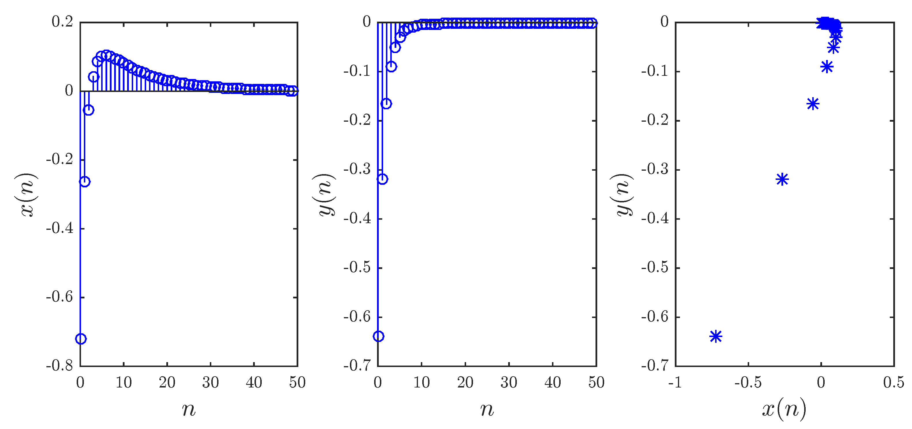
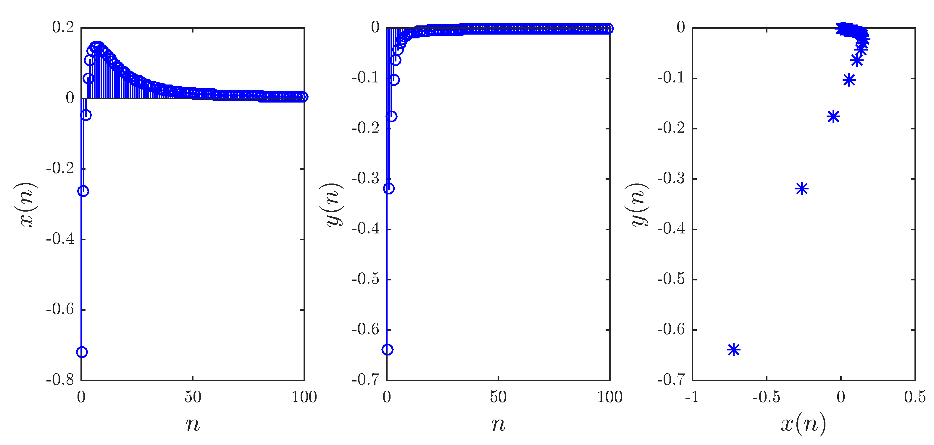
The result of Theorem 2 can be easily put to the test. Consider, for instance, parameters
, initial conditions
, and fractional order
. Using a modified version of the numerical formula (
8), we obtain the states depicted in
Figure 8. Clearly, the states do converge towards the all-zero solution. Although the convergence was only established for the commensurate case, experiments have shown that the proposed control laws are also valid for the incommensurate case.
Figure 9 shows the controlled states with the same parameters and initial conditions from above, but with different fractional orders
. Again, we see that the states do in fact converge towards zero, indicating successful stabilization. However, it is apparent that the convergence happens faster in the commensurate case where
.
5. Conclusions
In this paper, we have considered a fractional Caputo-difference form of the standard Tinkerbell chaotic map, which is well known for its rich dynamics and interesting characteristics. The dynamics of the fractional Tinkerbell map were investigated numerically using phase plots, bifurcation diagrams, and Lyapunov exponents. Through this investigation, we observed that the fractional order has a significant effect on the fractional map’s dynamics. This confirms what has been reported previously in the literature and suggests that the fractional map is superior to the standard one, as it includes more degrees of freedom.
We have also introduced a feedback linearization stabilizing controller for the proposed map and established the asymptotic convergence of the states towards the all-zero solution by means of the stability theory of linear fractional discrete systems. The success of the proposed scheme was demonstrated through numerical simulations both in the commensurate and incommensurate cases.
Although feedback linearization is simple to design and implement, its practicality has been challenged by many in the control and cybernetics research communities. For future work, we plan to investigate other control schemes that can perform better in terms of the power consumption and other essential criteria. The main challenge that we anticipate is the limited literature concerning the stability of fractional discrete systems, especially on the Lyapunov method. This would have to be addressed in order to be able to establish the convergence of any new control scheme.

 ,
, 


