1. Introduction
Megawatt-scale wind turbines are currently a mature technology. On one side, the current frontiers of research mainly deal with increasing the size of wind turbines and, therefore, the capacity factor, but there are still several open challenges (as, for example, the control of mechanical loads [
1,
2]) and, therefore, wind turbines having a rated power above 7 MW are, at their present state, mainly prototypes. On the other side, considerable attention has recently been devoted to the optimization of operating wind farms featuring megawatt-scale wind turbines. The optimization problem can involve the mutual interaction between the wind turbines or can deal with the energy conversion efficiency of each wind turbine. As regards the former issue, the fields of research are layout optimization [
3,
4,
5,
6,
7], cooperative wind turbine control [
8,
9,
10], and yaw active control for wake mitigation [
11,
12,
13,
14,
15]. As regards the latter issue, several types of wind turbines retrofitting for power production improvement are possible: They can be aerodynamic and based on the modification of the blade profile (installation of vortex generators, passive flow control devices, Gurney flaps, and so on [
16,
17,
18,
19,
20]), or they can involve the control system and deal with the management of the blade pitch [
21], the rotor rpm, the cut-out wind speed, and the high wind speed cut-in (defined as the wind speed at which the wind turbine starts producing again after a gust) [
22,
23,
24].
Certain attention has therefore been recently devoted in the scientific literature to the study of wind turbine power upgrades: The scientific interest is basically motivated by the fact that wind turbines operate under nonstationary conditions because the source is stochastic. Therefore, the impact of an upgrade cannot be estimated by simply studying the total production in pre- and post-upgrade periods. At least some meaningful indication can be obtained by studying how the wind turbine power curve (i.e., the relationship between wind speed and power output) changes after an upgrade. However, as discussed, for example, in Reference [
25], the study of the power curve might be insufficient for evaluating the impact of an upgrade. This can be due to the fact that the power of a wind turbine has multivariate dependencies (on climate conditions and on working parameters) and the study of the power curve disregards them all, except for wind speed and, possibly, air density [
26]. Furthermore, another problem regarding the study of the power curve is that wind speed is commonly measured through cup anemometers placed behind the rotor and the undisturbed wind speed is estimated by the wind turbine control system through a transfer function, generally computed from field campaigns in flat terrain. This implies that the precision of the wind speed measurements in complex environments might not be enough in order to distinguish a variation of a wind turbine power curve that is of the order of few percents.
This problem has therefore stimulated some interesting studies in the scientific literature about the ex-post assessment of wind turbine power upgrades through the analysis of operational data. For example, in Reference [
25], a modification of the Gaussian kernel regression method [
27] is proposed for computing the impact of two wind turbine upgrades: Pitch optimization and vortex generator installation on the wind turbine blades. The former test case is generated artificially by synthesizing the data according to the logic of pitch angle optimization; the latter test case, instead, is studied through the operational data of a wind turbine. Vortex generator installation is studied also in Reference [
28]: The employed methods are the kernel plus of Reference [
25] and the so-called power-power approach. The power–power approach is based on the study of the variation (before and after an upgrade) of the power difference between the wind turbine of interest (the target) and a reference wind turbine. Its weakness consists of the fact that it needs vast data sets in order to provide meaningful results: The authors of [
28] have addressed this problem by employing time-resolved data sets with sampling time of the order of the second, rather than ten minutes, like the typical Supervisory Control And Data Acquisition (SCADA) data. Some proposals to overcome this issue have been formulated in References [
21,
29]: The idea is that the power–power approach can be generalized by modeling the power of the wind turbine of interest as a function of operation variables of more than one reference near wind turbines. If an upgrade has a non-negligible effect on the performances of the wind turbine, it can be detected as a variation in the behavior of the residuals between model estimates (when the model is trained with pre-upgrade data) and measurements.
A common lesson arises from the above discussed studies: It is important, when possible, to study wind turbine power curve upgrades in real environments because the flow conditions at the microscale level can be relevant for the efficiency of the upgrade. At the same time, it would be important and cost-saving to have reliable estimates of the impact of wind turbine power upgrades that are based on numerical models or simulations. The objective, on one hand, is having at our disposal a second piece of advice to the data-based validation. On the other hand, if a model is reliable for estimating the impact of an upgrade, it can be used as a first or preliminary piece of advice before the installation of the upgrade. The present work deals exactly with this kind of problems. A real test case is studied: A multi-megawatt wind turbine sited in Italy in a considerably complex terrain has undergone optimization of the rotor rpm management in order to reach the most appropriate induction level. The objective of the work is twofold:
Employing operational data to provide an estimate of the impact of the upgrade after some months of operation;
validating a purely numerical framework (based on aeroelastic simulations of the wind turbine of interest) for estimating the impact of the control optimization.
The data-driven method is formulated on the grounds of the discussion in Reference [
30]: A multivariate linear model is selected, whose target is the power of the upgraded wind turbine and whose input variables are operation variables (power, rpm, blade pitches, and so on) of the nearby wind turbines. The input variables are selected based on their statistical significance by means of a stepwise regression algorithm [
31].
The aeroelastic simulations were performed using the open-source FAST (fatigue, aerodynamics, structures, and turbulence) v8 software, developed at the National Renewable Energy Laboratory (NREL) in Golden, Colorado. The control upgrade was taken into account in the simulations based on the generator rpm–generator torque curve, by mimicking the operational curves before and after the upgrade. Several aeroelastic simulations were run: From these, it was possible to estimate an average pre- and post-upgrade power curve. By weighting these power curves against wind distribution, the impact of the control upgrade on the production was estimated.
The main result of this work is that the data-driven and the numerical estimates of the upgrade display a good level of agreement. This result supports the use of numerical simulations for studying this kind of control upgrades, once they are fed with some input that is specific to the site (for example, turbulence intensity, wind intensity distribution) and to the technology (in this case, rotor rpm–power curves before and after the upgrade).
Summarizing, the structure of the manuscript is the following: In
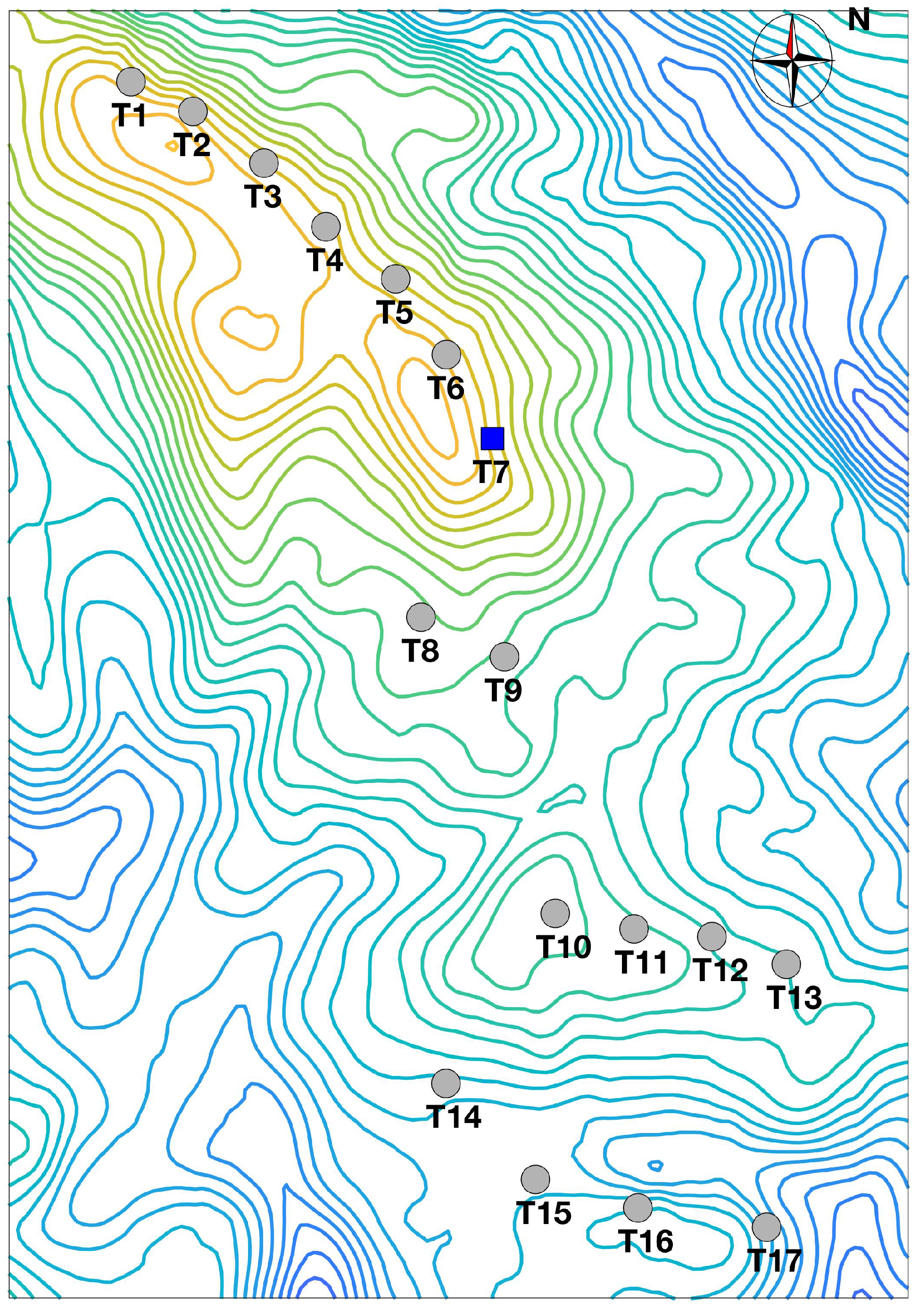
Section 2, the test case is briefly described.
Section 3 is devoted to the production improvement estimate based on operational data analysis: The method and the results are presented.
Section 4 is devoted to the upgrade assessment based on the numerical simulations: The framework and the results are described. Finally,
Section 5 is devoted to conclusions and some further direction of this work.
3. Operational Data Analysis: Methods and Results
The data sets at disposal are the following:
goes from 1 September 2017 to 1 March 2018. It is a period during which the standard rotor rpm–power curve was operating.
goes from 1 March 2018 to 1 July 2018. It is a period during which T7 was operating with the improved rotor rpm–power curve.
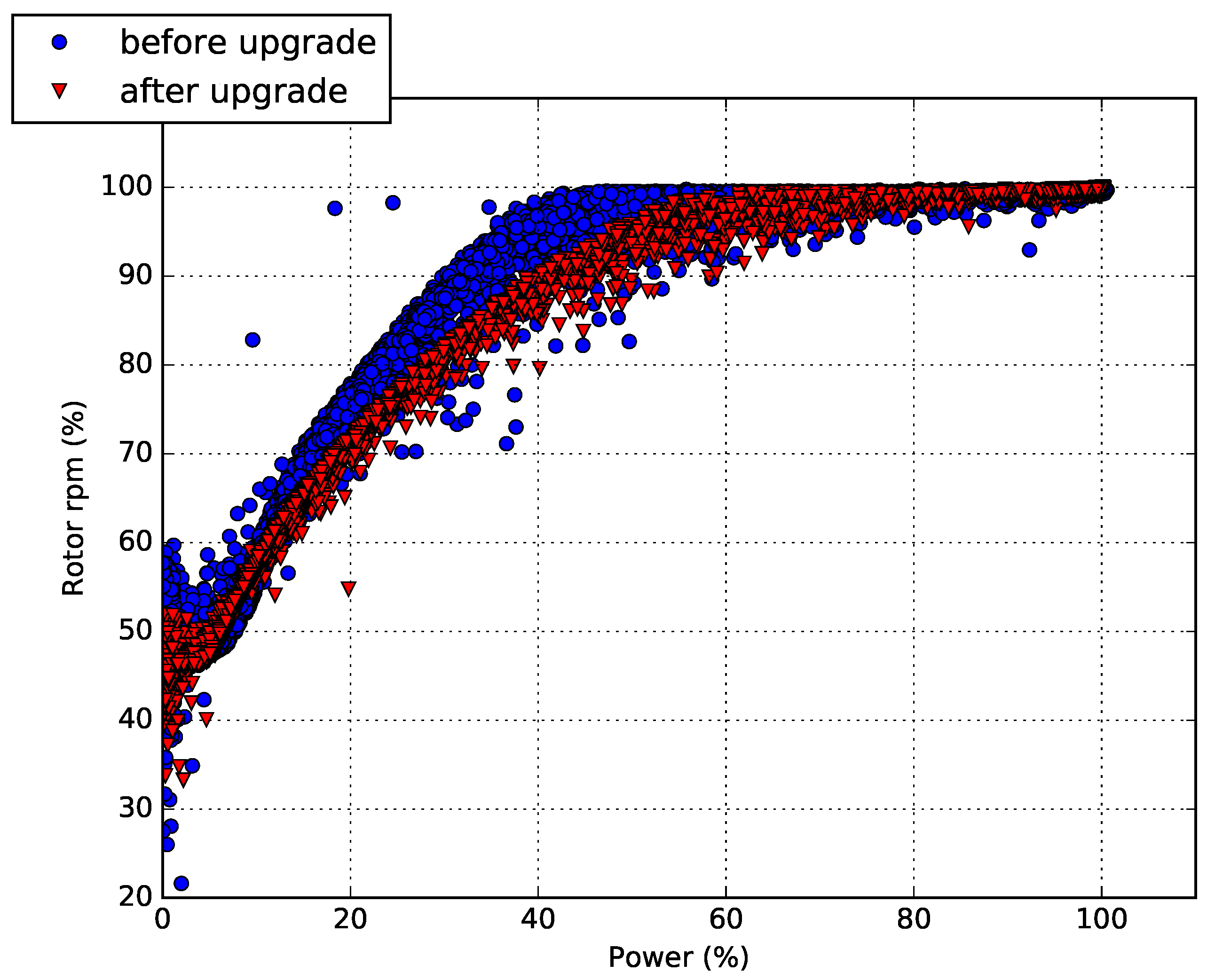
In
Figure 2, the power–rotor rpm curve for, respectively, the data sets
and
is reported. The difference between the two is appreciable: After the upgrade, a lower rotational speed was needed to extract the same amount of power as before the upgrade.
Unfortunately, it was impossible to study the impact of the upgrade using the power curve analysis. As discussed, for example, in Reference [
30], the T7 wind turbine underwent an aerodynamic retrofitting: Vortex generators and passive flow control devices were installed on the blades. After this intervention, prior to the control upgrade, the wind speed measurements at turbine T7 provided by the control system were biased: This is discussed in Reference [
30] through the study of the power factor
. Therefore, without a reliable wind speed measurement at turbine T7, it was impossible to study the power curve and the effect of the upgrade must be estimated using other methods.
The objective is therefore to estimate the power output of T7, denoted as y in the following, as a function of on-site conditions. Given the fact the wind speed measurements at T7 are unreliable and the operating parameters of T7 cannot be used in this task (because they change for given wind conditions, after the control upgrade), the critical point is deciding what variables opportunely define the on-site conditions and the relation between them and the power of T7. The decision is possibly to employ all the other 16 wind turbines in the farm as reference; the following measurements are available and can in principle be selected as input variables for modeling the power output of T7:
The nacelle wind speed,
the power output,
the individual blade pitch angles,
the rotor revolutions per minute,
the generator revolutions per minute,
the high speed rotor temperature.
The rationale is that if one trains a model with pre-upgrade data and validates it against a pre- and a post-upgrade data set, a difference should arise in the behavior of the residuals if the upgrade is really effective. One of the most important points in this kind of procedure is having an argument for selecting the most appropriate input variables for the model among all the possible measurements at our disposal in the wind farm. This problem is solved based on the stepwise regression algorithm [
31]: It is an iterative algorithm for automatically selecting the most appropriate inputs for a multilinear regression task. Starting from an initial model, at each iteration of the algorithm, an input term is added to or removed from the model. The decision about keeping it, removing or restoring it is based on the
p-value of an
, i.e., by testing the performance of the model with and without that potential term. If one input variable has a
p-value which is greater than an exit tolerance (that is, if it is unlikely that the hypothesis of a zero coefficient in the linear model can be rejected), that variable is discarded. Therefore, it is important to study the results of the stepwise regression algorithm: Basically, the idea is that a loose bound (high values) on the
p-value leads to larger models that reliably produce lower errors but are less solid, while a strict bound (small values) on the
p-value leads to smaller models that can produce higher errors but are more solid. In this case, selecting a compromise is quite easy based on
K-fold cross-validation [
35] for the sensitivity study of the
p-value selection. The procedure goes as follows: The data set
is divided
J times randomly in two subsets.
of the data are used for training and the remaining
are used for validation.
K is selected to be 10 for this study, because short validation folds stretch the capabilities of the model to the limit. J has been set to 300 to increase the statistical significance of the study. The performances of the linear model are quantified for each of the
J runs of the cross-validation for a given
p-value in terms of the mean absolute error between model estimates and measurements. In this case, the main feature of the results of the cross-validation is the following: The order of magnitude of the mean absolute error does not vary considerably when varying the
p-value, while the input selection sensibly depends on the
p-value. In particular, for a large
p-value, the model is not as stable as for a small
p-value: When the
p-value is large, several different final input selections are obtained along the
J runs of the cross-validation. This behavior (in particular the fact that the mean absolute error saturates quickly to a lower bound) can probably be interpreted as the effect of the remarkable complexity of the terrain and therefore of the wind flow (discussed by other points of view, for example, in References [
32,
33]). Therefore, the final decision is for a stable model that is obtained when
p-value
. Notice that
p-values up
have been tested: Therefore, the choice should be considered solid. The selected input variables for modeling the power of T7 are:
The power of T6;
the power of T9;
the rotor rpm of T8.
This input variable selection is reasonable: In the wind energy literature, it is widely discussed that the low precision of nacelle cup anemometers leads to the idea of using wind turbine rotors (and therefore, power and/or rpm) as probes of the wind conditions [
36]. Furthermore, T6, T8, and T9 are the nearest wind turbines with respect to T7, although T8 and T9 are sited at a quite different altitude. The resulting model can easily be interpreted as a generalization of the power–power method, because a model has been obtained for the power of the target wind turbine (T7) as a function of meaningful variables of three references nearby wind turbines (T6, T8, T9), instead of only one.
The procedure therefore goes as follows: Input measurements are normalized and organized in a matrix
. The pseudo-inverse of
is used to compute the weights of the linear regression model as:
where
is a column vector and
is the column vector of the T7 power measurements in the training data set. Finally, the estimated power output vector
on a given validation data set is computed as a linear combination of the input variables, weighted using
:
The data set is appropriately pre-filtered: The request is that the wind turbines T6–T7–T8–T9 (input and output of the model) are producing output and that the power of T7 is below rated. This second condition is requested because an upgrade is not effective when the produced power is rated.
The procedure to compute the effect of the upgrade is the following. The data sets at disposal are organized in this way:
is randomly divided in two subsets: D0 ( of the data) and D1 ( of the data). D0 is used for training the model and constructing the weight matrix , and D1 is used for the pre-upgrade data set employed for validating the model.
is the post-upgrade data set employed for validating the model. For notation consistency, it is also referred to equivalently as D2.
The residuals between the measurement
y and the simulation
, for the data sets D1 and D2, are studied. The focus is on how the residuals vary after the upgrade. Therefore, consider Equation (
3) with
.
For
, one computes:
The quantity is a percentage estimate of the production improvement.
It is possible to repeat the above procedure several times: This kind of bootstrap technique allows to simulate the repeatability of the tests. This is done as follows: At each run of the model, a different D0 (training set) and D1 (pre-upgrade validation dataset) are selected, while the whole D2 is kept as a validation data set at each run. One could decide to randomly select a subset of D2 as the post-upgrade validation data set but, in this work, the decision has been to take it fixed as a whole because it is shorter than the pre-upgrade data sets.
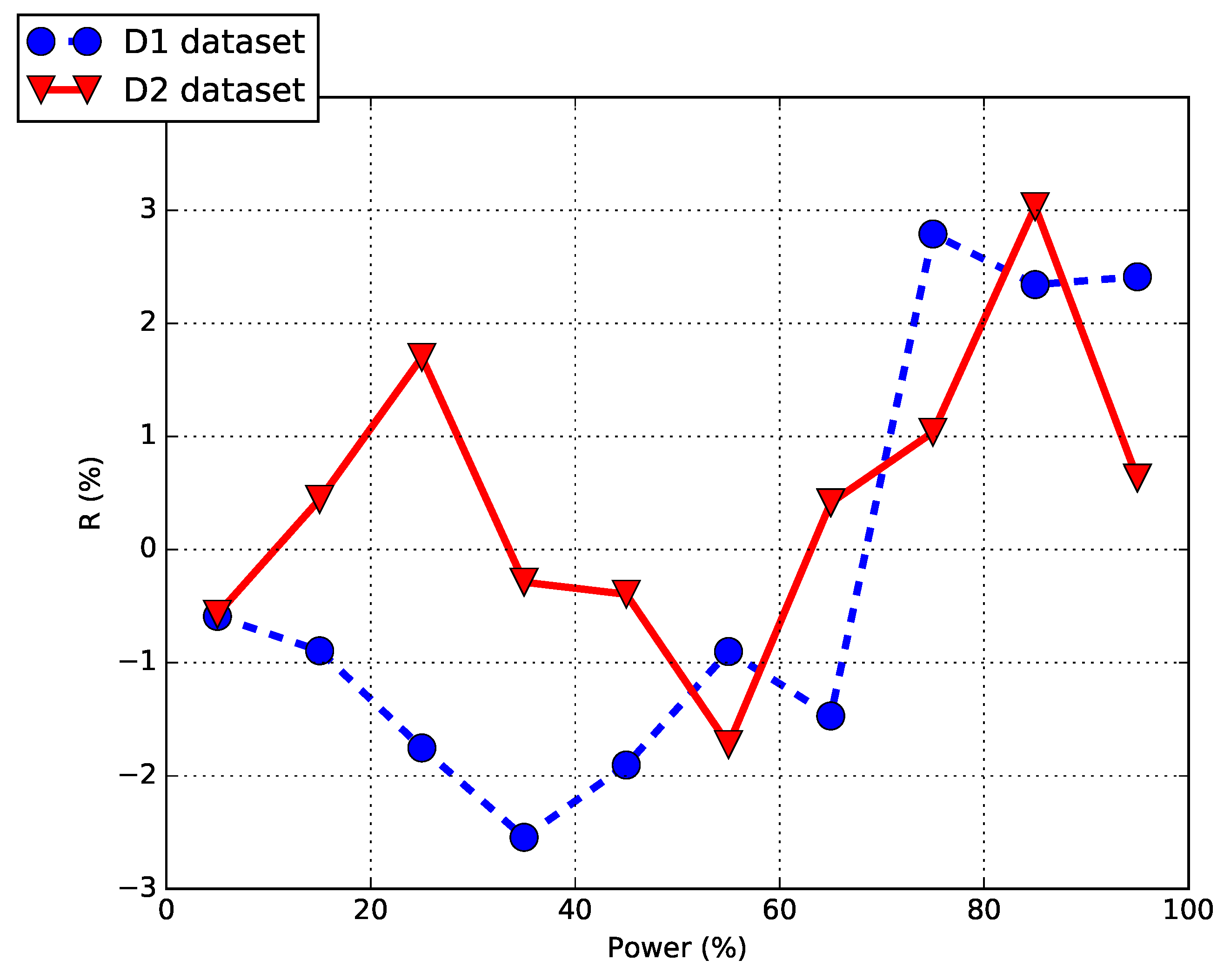
In
Figure 3, for a sample selection of D1, the sets
and
are plotted after being averaged in intervals of 10% of the rated power.
Figure 3 is consistent with the intuitive expectation about the upgrade of interest: The effect of the upgrade is visible below rated power (i.e., before the rpms saturate) as a change in the mean difference between measurements and model estimates. When the rpms saturate, approaching rated power, the residuals between model estimates and measurements have a similar behavior because the upgrade is not effective.
Basically, for each run of the model, an estimate of the energy improvement
can be obtained from Equation (
4): This procedure has been repeated several times and the average energy improvement is computed as
. In other words, the estimate is that T7 has produced, after the adoption of the control system upgrade, 1.0% more than it would have done without the upgrade. Recall that this percentage refers to the production below rated power, consistently with the adopted criteria for filtering the data sets. If one wants to estimate how much this improvement amounts to in terms of annual energy production, one can assume a certain wind distribution or deduce it from long-term data and project the
estimate on the data set of interest.
4. Numerical Analysis: Methods and Results
As discussed in
Section 1, this work deals with a twofold approach to the estimate of the power production improvement provided by wind turbine control upgrades. A validation on the basis of numerical simulations is provided: The aeroelastic code FAST v8 [
37], developed at National Renewable Energy Laboratory, is selected.
A detailed model of the wind turbine has been set up, in particular in terms of the aerodynamics of blades (that have been tuned thanks to the open source code QBlade [
38]) and elastic properties of blades and tower, according to the information available in Reference [
39] for the wind turbine model of interest for this study. The turning point for the purposes of this study is the representation of the control system (especially in terms of coupling with the electric generator), needed for the code to run the simulation. The approach called “Simple Variable–Speed Torque Control” has been chosen for modeling the relationship between torque and rpm: It is particularly useful, given the peculiarity of the data at our disposal (no reliable wind speed measurement is available at the site of the wind turbine of interest, as discussed in
Section 3), because it does not require the relationship between wind and power. Actually, the relationship between generator rpm and produced power
P (assuming an unitary efficiency, in order to use the relationship
to compute the mechanical torque
) is taken from the operational data before and after the upgrade (data sets
and
) and is reproduced in the numerical simulations. The FAST code represents this relationship with approximations in three power regions. A quadratic polynomial from zero power to maximum-power control is used (called “Region 2”), while at rated power, a constant value of torque is set (called “Region 3”). These two regions are connected by a very short interval of linear transition (called “Region
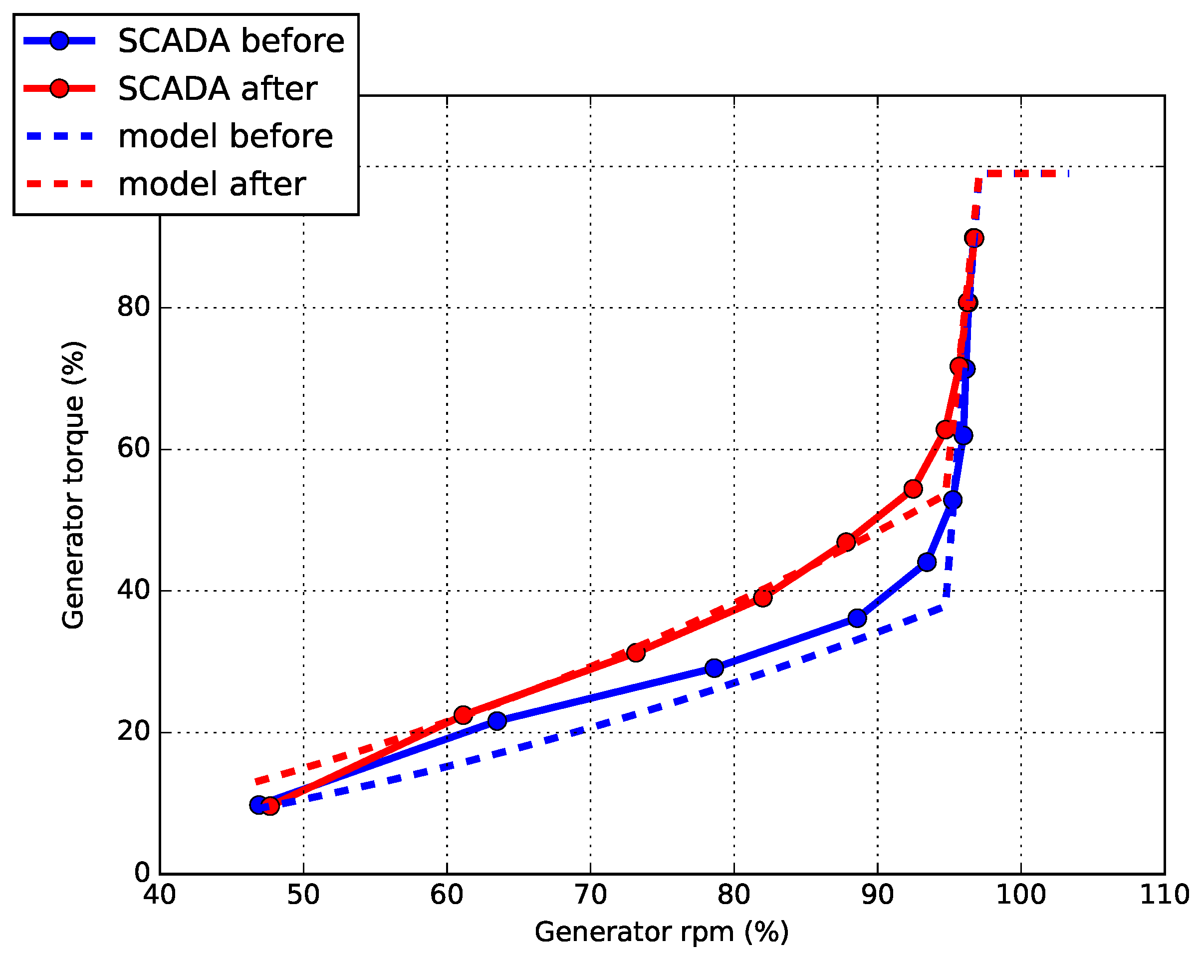
”). The approximation functions and the values of transition between the regions are fitted to the operational measurements before and after the upgrade: The result of this procedure is reported in
Figure 4, where the average experimental and simulated generator rpm–generator torque curves before and after the upgrade are shown. Notice that the post-upgrade average curve is more regular than the pre-upgrade and for this reason, the fit results to be more precise. This fact can also be seen from the operational data reported in
Figure 2: Computing the average and the standard deviation of the rotor rpm per power intervals, the result was that the percentage standard deviations was lower after the upgrade. This means that the control upgrade has improved the stability of the curve through a more appropriate selection of the rotor rpm as a function of the tip speed ratio.
Once the pre- and post- upgrade model have been tuned, the following step is the simulation of the wind speed and, consequently, of the electrical power. The decision has been to simulate several time series and the average wind intensities are selected to span from cut-in to rated with 0.5 m/s intervals. This has been done in order to resemble the typical wind speed spacing of the average power curve computed according to the IEC guidelines [
26]. The time series were generated using the TurbSim package and an A turbulence class was selected because, on the basis of the data at disposal for this study (despite the fact that their sampling time is 10 min), it was evaluated that the site is considerably turbulent. A wind shear exponent of 0.2 was selected because it is a good approximation for onshore wind farms.
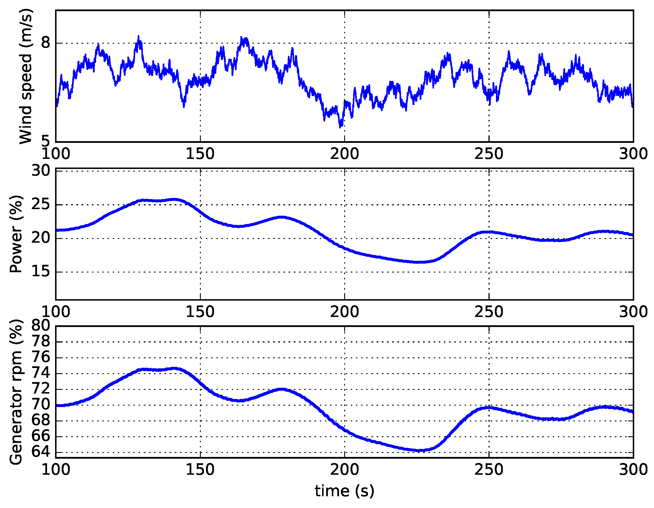
Each run of the model simulates 400 s with a time step of the millisecond: In
Figure 5, examples of wind intensity, rotor rpm, and power time series are reported.
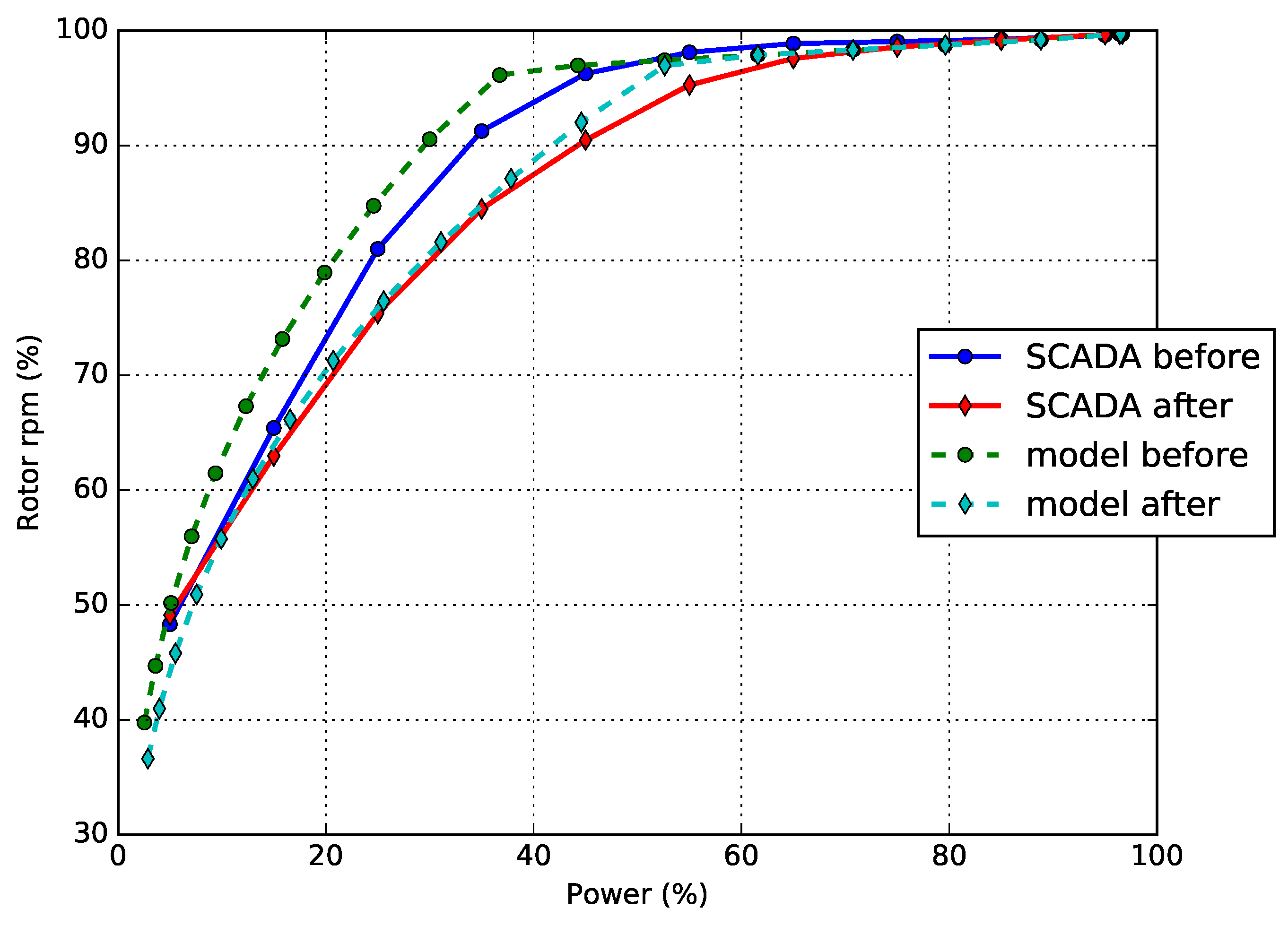
Subsequently, for each simulation, the average rotor rpm and electric power are computed: In
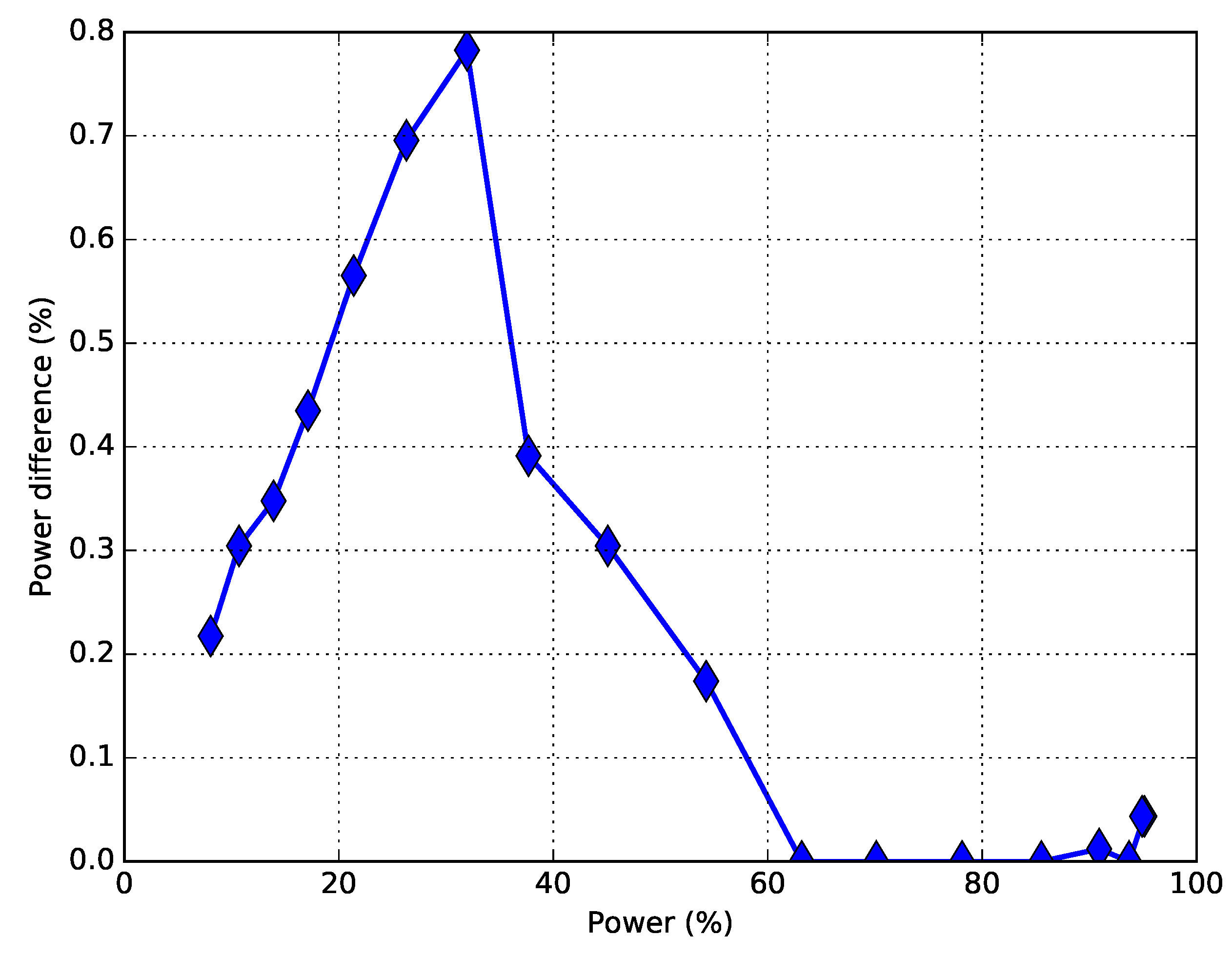
Figure 6, the simulated and measured rotor rpm–power curves are reported. This basically allows to simulate the power curve for the wind turbine before and after the upgrade. For the purposes of this study, it is very interesting to estimate the difference (
) between the two configurations, as shown in
Figure 7 in percentage of rated power.
The production improvement is clearly visible below rated power (especially up to more or less 50% of the rated power) and saturates quickly to zero, approaching rated power. This is basically consistent with the results in
Section 3, like, for example,
Figure 3, where the difference in the residuals is clear up to 50% of the rated power and oscillates around zero, approaching rated power. These average power differences are finally employed to estimate the impact on the on-site production by weighting them against a historical wind intensity distribution: Doing this, the final estimate is 0.9% of improvement of the production below rated power. It is interesting to notice that this estimate is compatible within the 10% with the one of
Section 3 based on operational data elaboration.
Moreover, the results of this work shed light on the perspective of reliably employing numerical simulations for assessing wind turbine control upgrades. A completely general framework, like aeroelastic simulations, can be adapted to simulate a real upgrade of a real wind turbine in a real environment by empowering it with information relatively easily obtainable: Some information about the flow features on site (basically, the level of turbulence), the mechanical and aerodynamic properties of the wind turbine of interest, and how the control upgrade acts (in this case, the rotor rpm–power curves).
5. Conclusions
This work has been devoted to the numerical and data-driven study of a wind turbine control upgrade. The selected test case is a rotor rpm management optimization on a multi-megawatt wind turbine, from a wind farm sited in Italy in a very complex terrain, featuring 17 aerogenerators. There were at least two major motivations for this study. The former motivation was that the efficiency of wind turbine power upgrades can depend remarkably on site-specific conditions and it is therefore important to formulate reliable data-based models for assessing them and to collect test cases discussions. The latter motivation is that validating numerical frameworks for reliably simulating wind turbine control upgrades in a real environment would be a major step forward for the industry and for the scientific community as well.
On these grounds, in this work, the test case was studied with a twofold approach. The objective was estimating the production improvement using, respectively, aeroelastic simulations and operational data before and after the upgrade.
As regards the use of operation data, the adopted strategy was the formulation of a robust model for the power of the wind turbine of interest. The model has been trained with pre-upgrade data and validated against a pre-upgrade and a post-upgrade data set: If the model is precise enough to resolve the upgrade of interest, a difference in the behavior of the residuals between measurements and model estimates should be detected. In this work, the selected model for the power of the wind turbine of interest was a multivariate linear; a point of particular interest was the selection of the most appropriate input variables for the model: This was achieved using a stepwise regression algorithm and the selected input variables are powers and rotor rpms of nearby wind turbines. In the selected test case, the result was three reference wind turbines being employed.
The reliability of the numerical simulations was based on mimicking the measured (before and after the upgrade) generator rpm–generator rpm curves. The FAST software represents this relation through approximations (quadratic, linear, and constant) and the functions that fit best the operational data were selected for the set up of the control system in the numerical environment. Once the pre- and post-upgrade models for the wind turbine of interest were tuned, simulations ere run spanning the interval of wind intensities from cut-in to rated power: Average wind intensities spaced 0.5 m/s were selected. The flow conditions on sitewere taken into account, by selecting a class A turbulence in the simulation of wind time series through the TurbSim package.
The above discussion clarifies that the data-driven and numerical methods are based on very different philosophies. The former is more or less a black box, based on operational data and on the assumption of a linear relation between several input variables from reference wind turbines and the power of the wind turbine of interest. The latter moves from the principles of blade element momentum theory. It is interesting that these two different methods provide results that are of the same order of magnitude: The improvement is estimated as +1.0% of the production below rated power. These results therefore shed light on the possibility of successfully adopting numerical simulations for estimating the effects of wind turbine control upgrades.
Furthermore, it should be noticed that a reliable numerical environment can be used in a predictive way. Specifically, for this kind of problems, simulations can be employed to estimate the modification of the mechanical loads induced by the control upgrade. This is actually the main further direction of this work and is also particularly stimulating as regards the state of the art about these topics in the scientific literature: Since retrofitting technologies are at their first stages as regards usage in the industry, the cost–benefits analysis is commonly conducted only on the basis of the production improvement estimates, but it should instead also include an analysis of the impact of the upgrades on the residue lifetime of wind turbine components. Moreover, with the selected simulation tool, it is possible to also study other kinds of control upgrades that have recently been spreading in the wind energy industry, for example, pitch angle management optimization. Another interesting further direction of this work is the study of time-resolved operational data (as done, for example, in Reference [
28]), because they have sampling time of the order of the second or less: This kind of data would be a challenging testing ground for the reliability of the numerical simulations, also at the level of the output time series.
