1. Introduction
In recent years, the development and adoption of Automated Driving Functions (ADF) have substantially increased. All major OEMs have started to include various assisting features such as Lane-Keep-Assist (LKA), Adaptive-Cruise-Control (ACC), parking assist, traffic jam assist and others, into their fleets. All with the same goal, to provide the customer with increased safety and comfort. By definition, these systems represent level 1–2 automation with respect to the 6 levels of automation defined by the SAE [
1]. However, test vehicles with higher level of automation, enabling fully unsupervised driving on defined street networks, are used for promotion and advertisement of research capabilities. In addition, test applications for automated transport, still with a supervisor on board, have been launched.
Beside OEMs, various research groups are working on novel technologies which provide enhancements in safety and efficiency of passenger vehicles. On one side, we have advanced vehicle state estimation [
2,
3,
4], followed by safe and agile maneuvering in extreme conditions [
5], and improved control of steering feedback to the driver [
6]. On the other side, improved safety is considered in several areas, starting from a shared control system where the human and ADFs are working in synergy [
7], to research focusing on pedestrian safety [
8], and in the development of future human-machine interfaces that should reduce driver distraction [
9]. Optimal and efficient driving will play a huge role in the future of automation as more and more vehicles become aware of their dynamic surroundings [
10].
However, testing and validation of these functions and their complex interactions are still among the biggest challenges in the field. Demonstrating the reliability, safety, and robustness of the technology in all conceivable situations, e.g., in all possible scenarios under all potential road and weather conditions, has been identified as the main roadblock for product homologation, certification and thus commercialization. It is also well known and accepted that time and cost-wise it is not feasible to drive the required 240 million kilometers [
11] manually with every vehicle variant to achieve a proven-in-use certification. In addition, for every sensor and software update the same number of kilometers would have to be repeated.
The focus of recent research in this area has been the development of methods and tools that reduce the number of driven kilometers for certification [
12]. Currently, the main expectation is that only a clever combination of methods selecting the important test-cases and test-environments including Software in the loop (SiL), Hardware in the loop (HiL), Vehicle in the loop (ViL) and test-track and public road will lead to a feasible reduction in current testing efforts. It is clear that many kilometers will be driven purely virtually. The advantages of virtual tests are, beside others, the independence from real time and the possibility to execute the tests in a safe and repeatable environment.
Nevertheless, the behavior of the ADFs needs to be continuously assessed and monitored throughout the whole tool chain. The data need to be classified by scenario type and severity level of safety and/or comfort issues. Currently, the classification is based on heuristic algorithms [
13,
14], where engineering experts spend a lot of time and effort to create the necessary rules. For each detected driving scenario, various Key Performance Indicators (KPI) are calculated to reflect the driving sensation of the passengers. However, some signal patterns are very challenging to be detected by heuristic algorithms only. There are no distinct triggers where a threshold could be set. Instead, the signals usually show decreasing and increasing slopes containing noise that could lead to misclassification. Furthermore, due to sensor noise or false target detections some information gets lost and therefore some interesting driving scenario cannot be detected correctly by the heuristics. This is where machine learning is applied to mend the detection rate when the networks, along with a well labeled dataset, have learned to deal with false positives and false negatives. The networks are not immune to data inaccuracy, but they are able to learn, to some degree, when the sensor measurements are inconsistent.
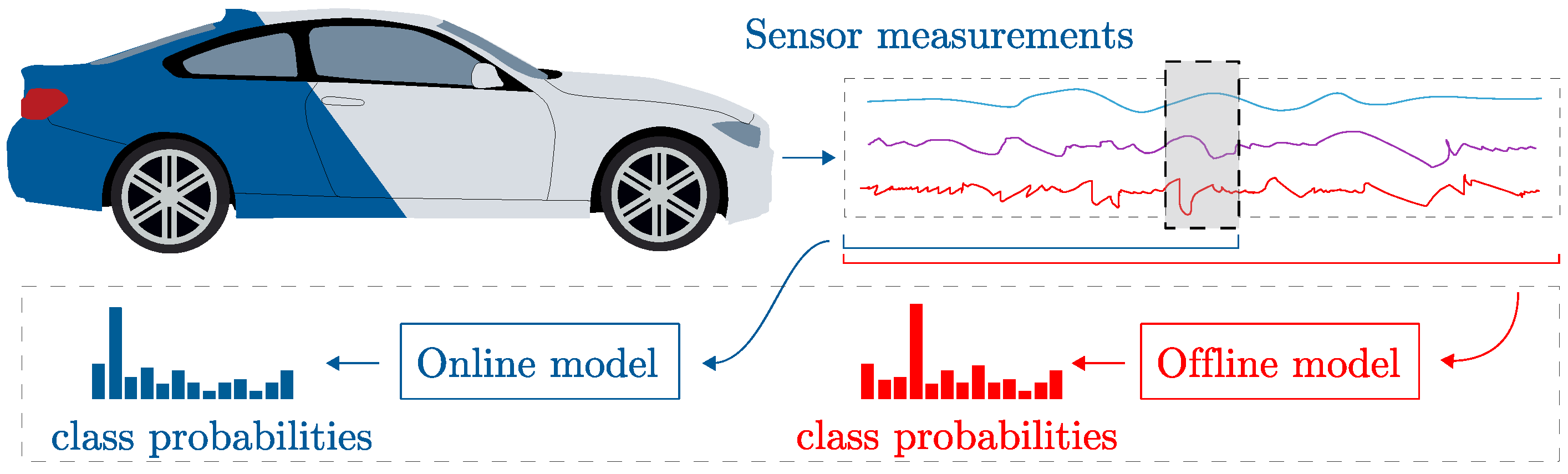
In this research we explore end-to-end Deep Learning (DL) methods for classification of driving scenarios related to LKA systems using time series data coming from various sensors. We focused on Convolutional Neural Networks (CNN) as they have shown better performance compared to Recurrent Neural Networks (RNN). Finally, we propose two classification models as shown in
Figure 1. The online model is used during driving, when a real-time classification is necessary. This model uses the past values to make the class predictions. The offline model is used in post-processing. As this model can use
a priori as well as
a posteriori knowledge in the recorded data, it can look what the vehicle was doing and then trace back and make the prediction. In other words, the model makes the prediction in the center of the considered time window taking in consideration what the vehicle did before and after. This approach leads to improved accuracy and can, to some degree, eliminate wrong detections.
2. Related Work
The most prominent driver for the development of deep neural network models capable of time series or sequence prediction and classification has been natural language processing and machine translation [
15,
16,
17]. The main idea behind it is to translate words, or phonemes if speech is used, into a fixed length vector embedding. This vector embedding can then be used as a time series sequence. The research resulting from the natural language processing is widely adopted to other fields that deal with time series data. Until recently, the
de facto choice for time series modeling have been RNNs. RNNs are networks that use hidden states that get propagated during time to compress valuable information from the past. Especially successful RNNs are the Long Short-Term Memory (LSTM) [
18] or Gated Recurrent Unit (GRU) [
19]. Both use several gates to control which information should be stored and which information should be forgotten.
Outside the natural language processing, the LSTM and GRU have been applied in various tasks such as general time series classification [
20], classification of ECG data [
21], time series forecasting [
22], etc.
Other researchers have also combined CNNs with RNNs to increase model performance. The main idea is to use the CNN in the first layers as feature extractors and later use RNNs for sequence classification. This method has been applied to trajectory clustering [
23], human activity classification [
24], sentiment classification [
25], and others.
However, RNNs have several limitations that can impact model accuracy and training duration. The training data for RNNs needs to be sequential and divided in such a way that the hidden outputs from one batch match the inputs of the next batch. This batching procedure could lead to deficient performance as some classes are only rarely seen by the network. Normally, shuffling of the data could greatly improve the training. However, shuffling of the data is not possible because we need to follow the constraint that each previous batch needs to lead to the current batch to preserve the propagation of the hidden states. In addition, RNNs process only one set of features at a time. After each step new hidden states and outputs are calculated which are then used in the next step. This sequential calculation procedure leads to increased training duration. CNNs do not suffer from these limitations. The data can be shuffled as individual batches do not have to be sequential. Furthermore, as the CNN is a feed-forward network the whole batch is processed directly.
The advantages of CNNs over RNNs have led researchers to apply only CNNs for time series classification [
26]; however, their performance has been inferior until recently. Bai et al. [
27] have shown that CNNs can produce even better results than RNNs if new architectural improvements such as dilatation and residual networks are used. Because of the recent breakthrough and their superior performance, we will focus on the usage of CNNs for the task of time series classification and compare their performance to RNNs.
Outside the scope of time series classification, CNNs have also been used for classification of driving scenarios. Gruner et al. [
28] proposed a spatiotemporal representation (Grid Map) that can capture dynamic traffic behavior. The representation is constructed using object information obtained by fusing data from several sensors. The representations are then used as inputs for a CNN which classifies the data into five classes:
Validity of frame,
Ego vehicle speed larger than 1m/s,
Leading vehicle ahead in lane,
Other vehicle overtaking the ego vehicle on adjacent lane,
Cross-traffic in front of the ego vehicle.
Our research differs from the mentioned methods as we perform time series classification using sensor data only. This data is used as an input to a CNN with separable and dilated convolutions, residual connections, and self-normalizing layers. In addition, we apply the network on a different classification problem, identifying driving scenarios relevant for LKA assessment.
3. Time Series Classification Using Convolutional Neural Networks (CNN)
This section will give an overview on the proposed model that consists of a CNN acting as a feature extractor which is followed by a dense multi-layer perceptron for classification. The convolutional feature extractor uses several enhancements compared to an ordinary CNN, which will be explained in the following subsections.
3.1. Depthwise Separable Convolutions
Given an input tensor with shape , where is the input depth or number of channels, and are the height and width respectively, an ordinary convolution layer applies the kernel over all the channels of the input tensor simultaneously and the whole kernel is applied for times leading to the output tensor with dimensions . Thus, the dimension of the kernel K is defined as , leading to a computational cost of . Generally, the convolutional layer filters input features and computes new representations at the same time.
On the contrary, the depthwise separable convolutions [
29,
30] separate the feature filtering and feature computation into two parts. For the filtering part, a separate convolutional kernel
is applied for each of the input channels
. As all the channels have their individual kernels an additional layer is needed to combine these filtered features. Thus, the depthwise convolution is followed by a
convolution generating the new representation. The
layer is a linear combination of the filtered features generated in the depthwise convolution. Each kernel
has a dimension of
and combined with the
convolution leads to a computational complexity of
. The number of parameters compared to the ordinary convolutional layer is reduced by the factor:
3.2. Dilated Convolutions
One drawback of ordinary CNNs is that, in order to achieve a wide receptive field, the networks need to be very deep. For example, if we have a 1D time series input and network with two convolutional layers, each with a
kernel and stride
(the kernel moves by 1 feature each step), the receptive field of the second layer will be 5. In other words, a perceptron in the second layer will be able to “perceive” 5 values from the input. In general, the receptive field grows linearly with the depth of the network and is given as:
where
and
are the receptive fields of the previous and current layer,
is the product over all previous strides and
k is the kernel size.
However, when working with time series data it is often necessary to consider a very wide view of the input to make adequate predictions. What if we could increase the receptive field of the network without adding more layers and increasing the size of the network? The solution is to use dilated convolutions [
31], as shown in
Figure 2. The main idea is that during the convolution the kernel is not considering every adjacent input from the previous layer but instead there is some fixed dilation step
between them. With this approach, it is possible to achieve an exponentially increasing receptive field formulated as:
It can be seen that the receptive field of the ordinary CNN (
2) is actually a special case of the dilated convolutional network (
3) where the dilation factor
equals 1. In practice, it is common to increase the dilation factor
exponentially for each layer
i, i.e., (
).
3.3. Residual Connections
To produce models that generalize well on highly complex data, the number of layers need to increase. By creating deeper models, and by using appropriate regularization, we assure that the models learn the necessary features to produce appropriate outputs. However, training deep networks represents a challenge because of the vanishing gradient problem. The gradients from the output layers need to be propagated through the whole network which makes the gradients closer to the input part of the network infinitely small, saturating and degrading the model.
He et al. [
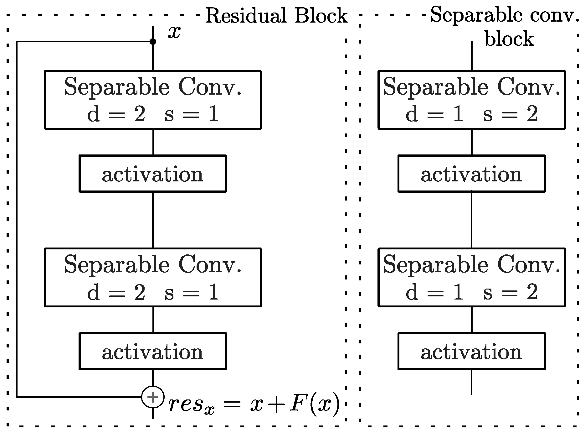
32] have proposed skip connections, as shown in the residual block in
Figure 3. The skip connection allows the network to learn a residual mapping more easily instead of the original underlying mapping, circumventing the gradient vanishing problem, as gradients can more easily flow through the network. However, Veit et al. [
33] have done research on the residual connections and argue that the skip connections allow the network to create better prediction as they effectively allow information to pass through different pathways.
The skip connection introduced in the residual block is basically an identity connection added to the convolutional layers and can be expressed with the following equation:
where
x is the layers input and
presents an ensemble of operations, in our case convolutional layers followed by an activation function.
3.4. Self-Normalizing Layers
It has become a widespread practice to use batch normalization [
34] between layers in CNNs to assure that layer outputs have zero mean and unit variance. This approach leads to faster training and serves as a regularizer for the network. However, a downside of batch normalization is that it increases the number of parameters of the network as they are used after each layer.
Klambauer et al. [
35] have introduced a new activation function called Scaled Exponential Linear Unit (SELU) that makes the layer’s outputs converge to zero mean and unit variance, naturally. This means that the usual batch normalization layer followed by nonlinear activation can be directly replaced by the SELU activation. The SELU activation is defined as:
where
and
are coefficients that determine the mean and variance of the layer’s output. Usually, their values are selected as
and
, which lead to zero mean and unit variance outputs.
If dropout [
36] is applied in the network than a special type of dropout called alpha dropout is needed to preserve the zero mean and unit variance between the layers. Together the SELU activation and alpha dropout lead to self-normalizing layers in the model.
3.5. Model Architecture
By applying the modifications to the ordinary convolutional network, we construct two models. One model for online and one for offline classification of scenarios. Both models share the same architecture but differ on how the input data is processed. The model architecture consists of a combination of two residual and two separable convolutional blocks, which are shown in
Figure 3. The eight convolutional layers are then followed by four dense layers. The parameters for each layer can be seen in
Table 1.
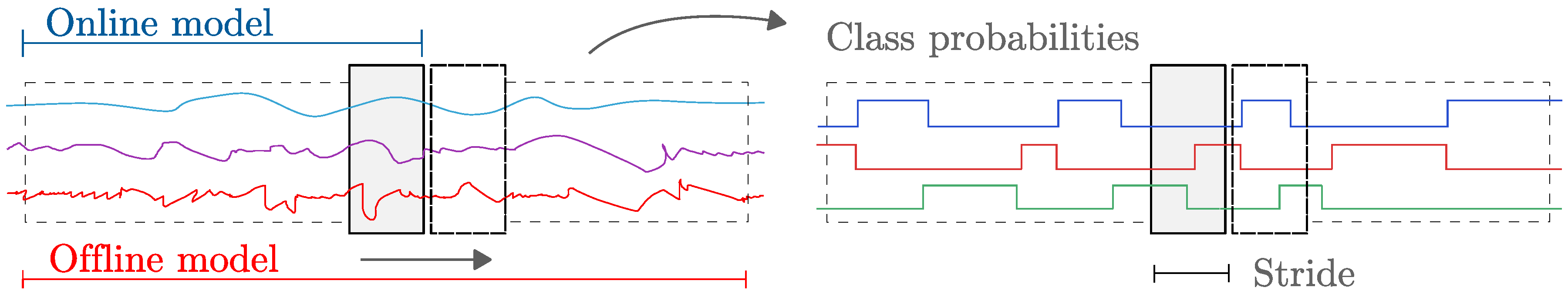
The input to the models is split into windows of equal length and move, with a fixed stride, through the time series data, as shown in
Figure 4. The online model is not able to “look” into the future and its input window consist of past measurements followed by the current stride. The model then uses this data to predict the classes associated with the current stride. When applied to real measurements on a vehicle, this scheme would result in a prediction for each stride duration, e.g., every half a second. The offline model has all the data available and thus can consider behavior of the vehicle before and after the current stride which leads to higher prediction accuracy.
4. Driving Data
The full dataset used to train the neural networks consists of real-world recordings obtained in seven highway and four motorway runs in the area around Graz, Austria. The dataset contains 183 channels and 304 thousand samples per channel, with a sampling rate of ten samples per second. The channels are raw sensor measurements coming from various sensors such as the lane detection camera, inertial measurement unit, encoders, etc., recorded directly from a CAN-Bus interface. As the focus of this research is classifying scenarios relevant for LKA systems, 10 relevant input channels were chosen to learn the distinct features. The used channels are: Lane Assist Lateral Deviation, Lane Assist Lateral Velocity, Lane Assist Lateral Velocity SMO20—smoothed with a 20-step window, Lane Curvature, Lane Width, Steering Wheel Angle, Longitudinal Acceleration, Lateral Acceleration, Velocity and Yaw Rate.
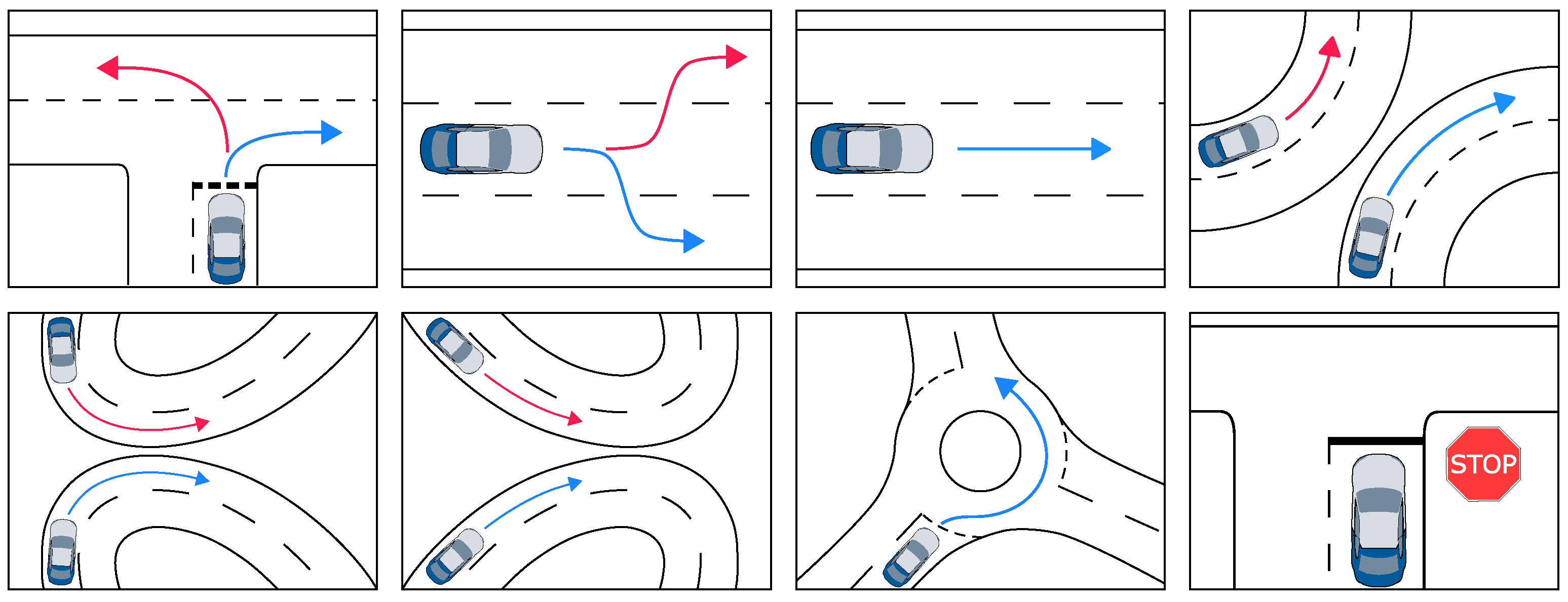
The model should learn to segment the data into 13 classes, as shown in
Figure 5, which were hand labeled using a custom labeling tool. The labels are:
TR: Turn Right,
TL: Turn Left—these two classes are defined with slow velocity sharp turns,
LCLR: Lane Change Left to Right,
LCRL: Lane Change Right to Left,
S: Straight—straight driving,
CL: Curve Left,
CR: Curve Right—curves with fixed radius,
TOL: Turn Out Left,
TOR: Turn Out Right—curves with increasing radius,
TIL: Turn In Left,
TIR: Turn In Right—curves with decreasing radius,
R: Roundabout and
SS: Stand Still. The labeled data contains class probabilities for each sample from the training data. When a sample could not be assigned to one of the thirteen classes, a uniform distribution between the classes was introduced to represent the unknown state. In other words, the model should not be able to tell which class the sample belongs to by generating low probabilities for all classes.
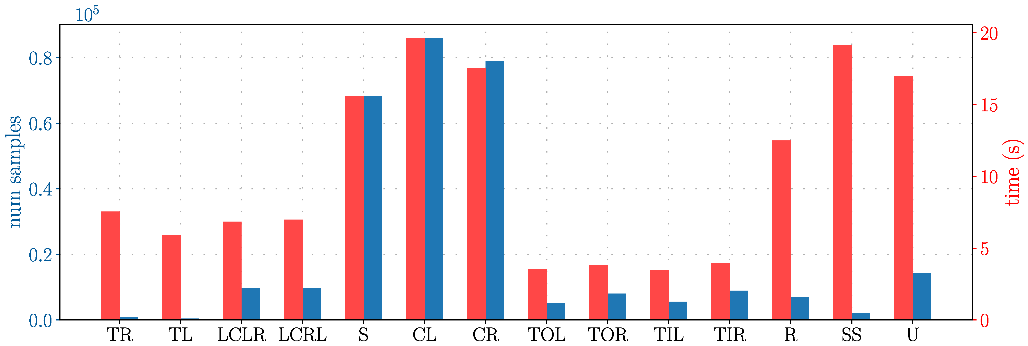
The distribution of samples per class is shown in
Figure 6. A strong imbalance between the classes exists which limits the capacity to train the models. Classes TR, TL and SS appear very rarely in the dataset, whereas S, CL, CR appear with a much higher occurrence. There was no possibility to balance the classes more evenly during the recording. In addition, various time series augmentation techniques were applied but they did not show any improvements on the accuracy of the models. Furthermore, time series data, such as the present one, contain classes which repeat for a long period of time, i.e., during parts of the training the network gets as an input only one class which hinders generalization. A remedy for this problem is to shuffle the data. However, shuffling of the data is not possible if RNNs are used. The requirement of these networks is that all data is introduced sequentially. CNNs on the other hand are applied on segments of the data, i.e., windows. Inside the windows the data is sequential but individual windows can be shuffled which increases the accuracy.
The average duration per class is shown in
Figure 6. This information is used to determine the size of the windows used for the CNNs. By increasing the window size, we increase the complexity, size, and accuracy of the models. However, if we increase the windows size to much the accuracy will decrease because we are not able to distinguish classes with shorter duration. On the other hand, if we use a small window size the network will not be able to learn the classification triggers for the classes with longer duration. After an experimental analysis we decided to use a window size of 8 s (80 samples) for the offline, and 6 seconds (60 samples) for the online model providing good balance between accuracy and complexity. In addition, both models use the same stride length of 5 s (5 samples) to traverse the windows over the whole data.
5. Results
The models were trained and evaluated using both the highway and motorway data. The first dataset contains only the highway records; whereas, the second dataset contains all recordings. In both cases, a test set including of the recorded data is left for the evaluation of the models after the training.
We compared the performance of the proposed CNN networks with two LSTM networks using the same window size and stride length. The first LSTM network is a multi-layer network with 3 layers and hidden state size of 512 neurons. The second LSTM network is a 3 layer bi-directional network with the same hidden state size. The bi-directional LSTM has twice as many neurons compared to the first LSTM network. One part of the biLSTM network starts at the beginning and traverses the input until the end, and the second part starts at the end and traverses the input to the beginning. This approach leads to better results as the network combines both the forward and backward pass to make a prediction.
All models were trained for 100 epoch using a decaying learning rate, with batch size of 256 samples. The CNNs use the Adam optimizer, whereas the LSTM networks use the Adagrad optimizer. To increase the generalization, a dropout rate of was applied to all models. For the LSTM networks the dropout was used on the 3 layers, and for the CNN networks the dropout was applied on the dense layers. In addition, the CNN networks use L2 regularization for the kernel weights with a regularization factor of .
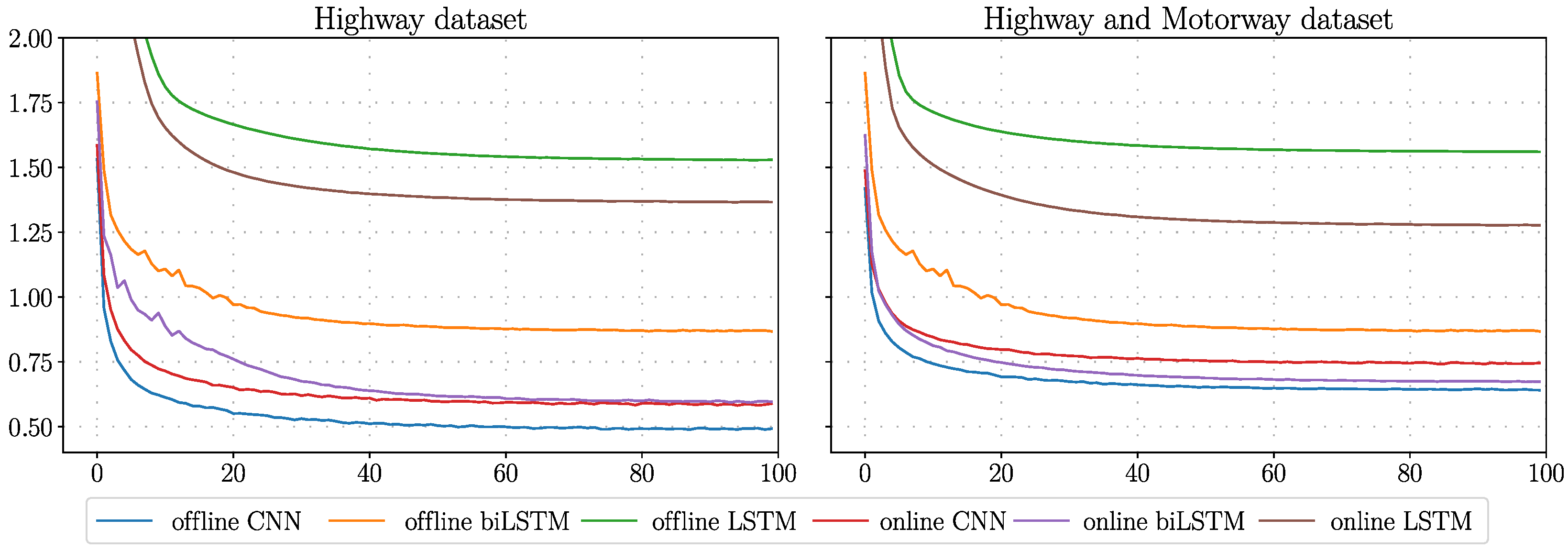
The training losses are shown in
Figure 7. The offline CNN model has the lowest training loss compared to all other networks. The LSTM network has the worst performance and the network is not able to model the data well. Compared to LSTM, the bi-directional LSTM has a much better performance. On the highway/motorway dataset the online biLSTM model performs better than the online CNN model. However, when comparing the offline and online bi-directional LSTM we can see that the offline models performs worse than the online one. A possible explanation could be that the offline model is not able to memories the “future” part of the data well when making a prediction in the middle of the window.
The accuracy of the models on the test sets can be seen in
Table 2. The columns present the evaluated models and the rows present the accuracy and loss for the highway, and highway/motorway datasets. We can see that the offline CNN has the best accuracy on both test sets. The online bi-directional LSTM has the lowest loss in both cases, but still a lower accuracy compared to the CNN. This is possible because the loss is calculated as the mean cross entropy loss, meaning that the bi-direction LSTM makes more mistakes in general, but the class probabilities are closer to the desired ones.
The decrease in accuracy between the highway, and highway/motorway dataset is due to the fact that the motorway dataset is more complex, and that the outputs from the sensors are not always consistent. In addition, because some classes are appearing less frequently than others, the models are not able to fully generalize.
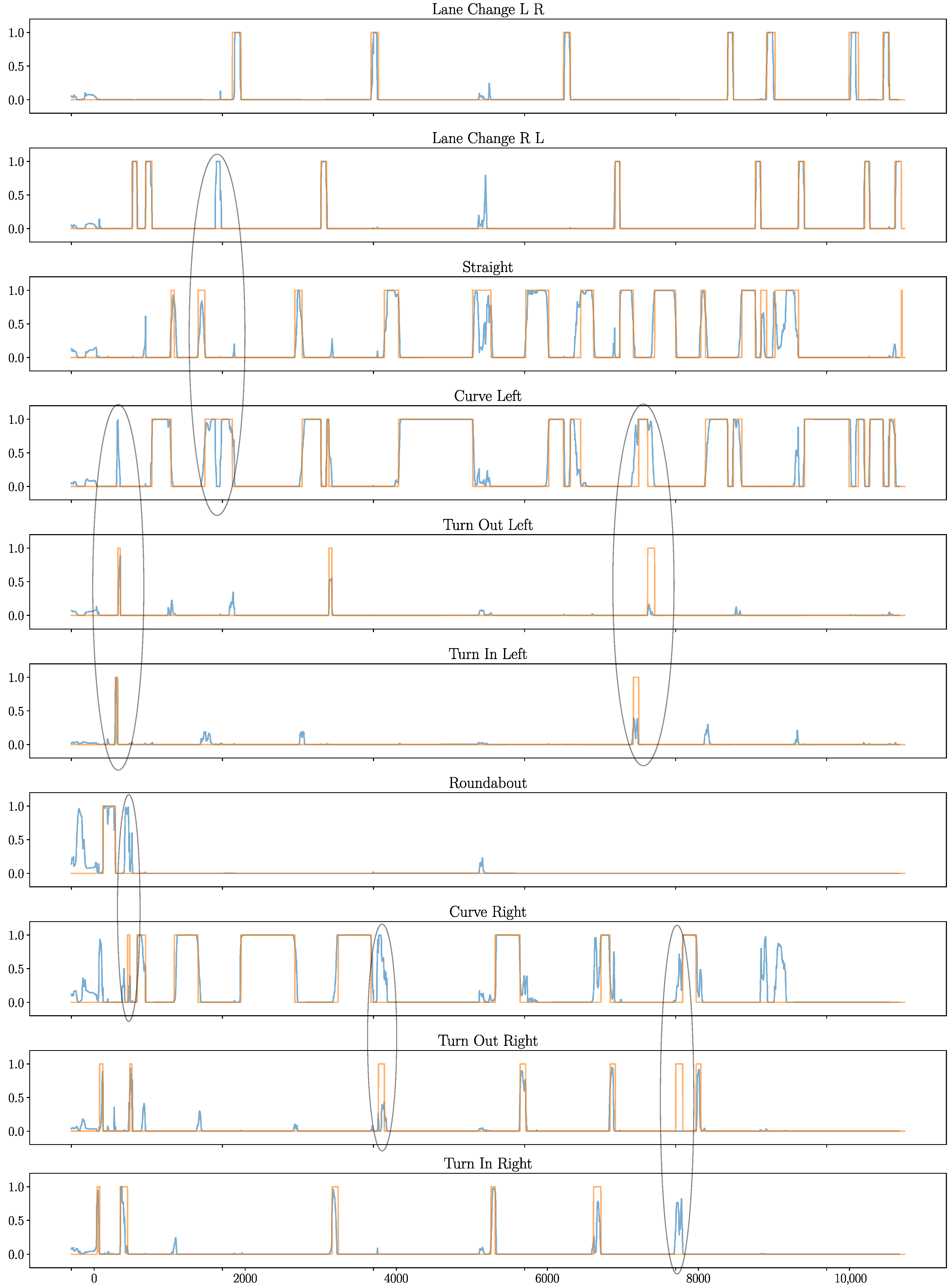
Figure 8. shows a part of the highway test set. We confirm that the model can distinguish the desired classes providing satisfactory results. However, some misclassifications are still present. The black ellipses in the figure highlight some of them. For example, the model confuses the CL class with TIL, TOR or LCRL. These classes are all very similar with subtle differences in the curvature radius or duration of the maneuver. In general, the accuracy and generalization of the model could be greatly increased if more balanced data is available.
6. Conclusions
In this paper, we applied end-to-end DL architectures for classification of driving scenarios used for evaluation of ADFs. We focused on scenarios relevant for LKA systems and considered both Convolutional (CNN) and Recurrent Neural Networks (RNNs). Through evaluation on two datasets, we concluded that CNNs provide better accuracy. Even though the performance of the proposed method is satisfactory, due to the imbalances of classes in the data, similarities between classes and sensor inconsistencies the networks could not fully generalize. However, we believe that deep neural networks represent a great tool for scenario classification as the complex classification rules can be learned directly by the networks. In addition, the accuracy of the networks can be increased incrementally as more data is recorded. In our future work, we will expand the number of classified scenarios taking into consideration also other traffic participants.
Author Contributions
Conceptualization, H.B., T.S., S.M. and M.H.; Methodology, H.B., S.M and M.H.; Software, H.B.; Validation, H.B. and T.S.; Formal Analysis, H.B.; Investigation, H.B.; Resources, H.B., T.S. and S.M.; Data Curation, T.S.; Writing—Original Draft Preparation, H.B.; Writing—Review & Editing, H.B., T.S., S.M. and M.H.; Visualization, H.B.; Supervision, M.H. and S.M.; Project Administration, M.S.; Funding Acquisition, S.M.
Funding
The project leading to this application has received funding from the European Union’s Horizon 2020 research and innovation program under the Marie Sklodowska-Curie grant agreement No. 675999.
Acknowledgments
The authors would like to thank Christian Wurzer for his work on the data labeling and initial LSTM tests.
Conflicts of Interest
The authors declare no conflicts of interest.
References
- SAE International. Taxonomy and Definitions for Terms Related to Driving Automation Systems for On-Road Motor Vehicles; SAE International: Warrendale, PA, USA, 2018. [Google Scholar]
- Vazquez, A.G.A.; Correa-Victorino, A.; Charara, A. Robust multi-model longitudinal tire-force estimation scheme: Experimental data validation. In Proceedings of the IEEE 20th International Conference on Intelligent Transportation Systems (ITSC), Yokohama, Japan, 16–19 October 2017; pp. 1–7. [Google Scholar]
- Regolin, E.; Zambelli, M.; Ferrara, A. Wheel forces estimation via adaptive sub-optimal second order sliding mode observers. In Proceedings of the XXVI International Conference on Information, Communication and Automation Technologies (ICAT), Sarajevo, Bosnia-Herzegovina, 26–28 October 2017. [Google Scholar]
- Ricciardi, V.; Acosta, M.; Augsburg, K.; Kanarachos, S.; Ivanov, V. Robust brake linings friction coefficient estimation for enhancement of ehb control. In Proceedings of the XXVI International Conference on Information, Communication and Automation Technologies (ICAT), Sarajevo, Bosnia-Herzegovina, 26–28 October 2017. [Google Scholar]
- Acosta, M.; Kanarachos, S.; Blundell, M. Vehicle agile maneuvering: From rally drivers to a finite state machine approach. In Proceedings of the IEEE Symposium Series on Computational Intelligence (SSCI), Athens, Greece, 6–9 December 2016; pp. 1–8. [Google Scholar]
- Chugh, T.; Chen, W.; Klomp, M.; Ran, S.; Lidberg, M. Design and control of model based steering feel reference in an electric power assisted steering system. In Dynamics of Vehicles on Roads and Tracks Volume 1: Proceedings of the 25th International Symposium on Dynamics of Vehicles on Roads and Tracks (IAVSD 2017), Rockhampton, QLD, Australia, 14–18 August 2017; CRC Press: Boca Raton, FL, USA, 2017; p. 43. [Google Scholar]
- Jugade, S.; Victorino, A.; Cherfaouii, V. Human-Intelligent System Shared Control Strategy with Conflict Resolution. In Proceedings of the IEEE International Conference on Control and Automation (ICCA), Anchorage, AK, USA, 12–15 June 2018. [Google Scholar]
- Hartmann, M.; Viehweger, M.; Desmet, W.; Stolz, M.; Watzenig, D. “Pedestrian in the loop”: An approach using virtual reality. In Proceedings of the XXVI International Conference on Information, Communication and Automation Technologies (ICAT), Sarajevo, Bosnia-Herzegovina, 26–28 October 2017. [Google Scholar]
- Aksjonov, A.; Nedoma, P.; Vodovozov, V.; Petlenkov, E.; Herrmann, M. A method of driver distraction evaluation using fuzzy logic: Phone usage as a driver’s secondary activity: Case study. In Proceedings of the XXVI International Conference on Information, Communication and Automation Technologies (ICAT), Sarajevo, Bosnia-Herzegovina, 26–28 October 2017. [Google Scholar]
- Ajanović, Z.; Stolz, M.; Horn, M. Energy-Efficient Driving in Dynamic Environment: Globally Optimal MPC-like Motion Planning Framework. In Advanced Microsystems for Automotive Applications 2017; Zachäus, C., Müller, B., Meyer, G., Eds.; Springer International Publishing: Cham, Switzerland, 2018; pp. 111–122. [Google Scholar]
- Winner, H.; Hakuli, S.; Lotz, F.; Singer, C. Handbook of Driver Assistance Systems: Basic Information, Components and Systems for Active Safety and Comfort; Springer: Berlin, Germany, 2016. [Google Scholar]
- Beglerovic, H.; Stolz, M.; Horn, M. Testing of autonomous vehicles using surrogate models and stochastic optimization. In Proceedings of the IEEE 20th International Conference on Intelligent Transportation Systems (ITSC), Yokohama, Japan, 16–19 October 2017; pp. 1–6. [Google Scholar]
- Holzinger, J.; Schloemicher, T.; Bogner, E.; Schoeggl, P. Objective assessment of comfort and safety of advanced driver assistance systems. In Proceedings of the FISITA World Automotive Congress, Busan, Korea, 26–30 September 2016. [Google Scholar]
- AVL-DRIVE® ADAS. Available online: www.avl.com/-/avl-drive-4- (accessed on 4 December 2018).
- Hermans, M.; Schrauwen, B. Training and analysing deep recurrent neural networks. In Advances in Neural Information Processing Systems; Curran Associates, Inc.: Red Hook, NY, USA, 2013; pp. 190–198. [Google Scholar]
- Sutskever, I.; Vinyals, O.; Le, Q.V. Sequence to sequence learning with neural networks. In Advances in Neural Information Processing Systems; Curran Associates, Inc.: Red Hook, NY, USA, 2014; pp. 3104–3112. [Google Scholar]
- Bahdanau, D.; Cho, K.; Bengio, Y. Neural machine translation by jointly learning to align and translate. arXiv, 2014; arXiv:1409.0473. [Google Scholar]
- Hochreiter, S.; Schmidhuber, J. Long short-term memory. Neural Comput. 1997, 9, 1735–1780. [Google Scholar] [CrossRef] [PubMed]
- Chung, J.; Gulcehre, C.; Cho, K.; Bengio, Y. Empirical evaluation of gated recurrent neural networks on sequence modeling. arXiv, 2014; arXiv:1412.3555. [Google Scholar]
- Malhotra, P.; TV, V.; Vig, L.; Agarwal, P.; Shroff, G. TimeNet: Pre-trained deep recurrent neural network for time series classification. arXiv, 2017; arXiv:1706.08838. [Google Scholar]
- Salloum, R.; Kuo, C.C.J. ECG-based biometrics using recurrent neural networks. In Proceedings of the IEEE International Conference on Acoustics, Speech and Signal Processing (ICASSP), New Orleans, LA, USA, 5–9 March 2017; pp. 2062–2066. [Google Scholar]
- Borovykh, A.; Bohte, S.; Oosterlee, C.W. Conditional time series forecasting with convolutional neural networks. arXiv, 2017; arXiv:1703.04691. [Google Scholar]
- Yao, D.; Zhang, C.; Zhu, Z.; Huang, J.; Bi, J. Trajectory clustering via deep representation learning. In Proceedings of the International Joint Conference on Neural Networks (IJCNN), Anchorage, AK, USA, 14–19 May 2017; pp. 3880–3887. [Google Scholar] [CrossRef]
- Ordó nez, F.J.; Roggen, D. Deep convolutional and lstm recurrent neural networks for multimodal wearable activity recognition. Sensors 2016, 16, 115. [Google Scholar] [CrossRef] [PubMed]
- Zhang, Y.; Er, M.J.; Venkatesan, R.; Wang, N.; Pratama, M. Sentiment classification using comprehensive attention recurrent models. In Proceedings of the IEEE International Joint Conference on Neural Networks (IJCNN), Vancouver, BC, Canada, 24–29 July 2016; pp. 1562–1569. [Google Scholar]
- Wang, Z.; Yan, W.; Oates, T. Time series classification from scratch with deep neural networks: A strong baseline. In Proceedings of the International Joint Conference on Neural Networks (IJCNN), Anchorage, AK, USA, 14–19 May 2017; pp. 1578–1585. [Google Scholar] [CrossRef]
- Bai, S.; Kolter, J.Z.; Koltun, V. An empirical evaluation of generic convolutional and recurrent networks for sequence modeling. arXiv, 2018; arXiv:1803.01271. [Google Scholar]
- Gruner, R.; Henzler, P.; Hinz, G.; Eckstein, C.; Knoll, A. Spatiotemporal representation of driving scenarios and classification using neural networks. In Proceedings of the IEEE Intelligent Vehicles Symposium (IV), Los Angeles, CA, USA, 11–14 June 2017; pp. 1782–1788. [Google Scholar]
- Howard, A.G.; Zhu, M.; Chen, B.; Kalenichenko, D.; Wang, W.; Weyand, T.; Andreetto, M.; Adam, H. Mobilenets: Efficient convolutional neural networks for mobile vision applications. arXiv, 2017; arXiv:1704.04861. [Google Scholar]
- Sandler, M.; Howard, A.; Zhu, M.; Zhmoginov, A.; Chen, L.C. Inverted Residuals and Linear Bottlenecks: Mobile Networks for Classification, Detection and Segmentation. arXiv, 2018; arXiv:1801.04381. [Google Scholar]
- Yu, F.; Koltun, V. Multi-scale context aggregation by dilated convolutions. arXiv, 2015; arXiv:1511.07122. [Google Scholar]
- He, K.; Zhang, X.; Ren, S.; Sun, J. Deep residual learning for image recognition. In Proceedings of the IEEE Conference on Computer Vision and Pattern Recognition, Las Vegas, NV, USA, 27–30 June 2016; pp. 770–778. [Google Scholar]
- Veit, A.; Wilber, M.J.; Belongie, S. Residual networks behave like ensembles of relatively shallow networks. In Advances in Neural Information Processing Systems; Curran Associates, Inc.: Red Hook, NY, USA, 2016; pp. 550–558. [Google Scholar]
- Ioffe, S.; Szegedy, C. Batch normalization: Accelerating deep network training by reducing internal covariate shift. arXiv, 2015; arXiv:1502.03167. [Google Scholar]
- Klambauer, G.; Unterthiner, T.; Mayr, A.; Hochreiter, S. Self-normalizing neural networks. In Advances in Neural Information Processing Systems; Curran Associates, Inc.: Red Hook, NY, USA, 2017; pp. 971–980. [Google Scholar]
- Srivastava, N.; Hinton, G.; Krizhevsky, A.; Sutskever, I.; Salakhutdinov, R. Dropout: A simple way to prevent neural networks from overfitting. J. Mach. Learn. Res. 2014, 15, 1929–1958. [Google Scholar]
Figure 1.
Concept overview. Scenario detection from sensor data using online and offline model.
Figure 1.
Concept overview. Scenario detection from sensor data using online and offline model.
Figure 2.
Visual representation of the dilated convolutional layers with different dilation factors d. It can be seen how the last layer has a wide receptive field.
Figure 2.
Visual representation of the dilated convolutional layers with different dilation factors d. It can be seen how the last layer has a wide receptive field.
Figure 3.
Building blocks of the CNN network. The residual block with dilated separable convolutions is shown on the left. The separable convolutional layers with stride for dimensionality reduction is shown on the right.
Figure 3.
Building blocks of the CNN network. The residual block with dilated separable convolutions is shown on the left. The separable convolutional layers with stride for dimensionality reduction is shown on the right.
Figure 4.
Window partitioning for class predictions. In the online model the input is only the current stride and an aggregated past. No information of what happened after the prediction is available. On the offline model the information what the vehicle did after the detection is available, enabling the model to make a prediction based on past and future behavior of the vehicle. To process the whole data, the windows are moved with a fix stride length generating corresponding class probabilities.
Figure 5.
Example scenario classes. From left to right, top to bottom the labels are: TR: Turn Right, TL: Turn Left, LCLR: Lane Change Left to Right, LCRL: Lane Change Right to Left, S: Straight, CL: Curve Left, CR: Curve Right, TOL: Turn Out Left, TOR: Turn Out Right, TIL: Turn In Left, TIR: Turn In Right, R: Roundabout and SS: Stand Still.
Figure 6.
Distribution and average duration of scenario classes.
Figure 6.
Distribution and average duration of scenario classes.
Figure 7.
Training losses for the online and offline models trained on the highway, and highway/ motorway datasets, respectively. CNN: Convolutional Neural Network, LSTM: Long Short-Term Memory, biLSTM: bi-directional Long Short-Term Memory.
Figure 7.
Training losses for the online and offline models trained on the highway, and highway/ motorway datasets, respectively. CNN: Convolutional Neural Network, LSTM: Long Short-Term Memory, biLSTM: bi-directional Long Short-Term Memory.
Figure 8.
Part of the highway test set with a duration of 20 min showing that the model can learn the desired class labels. Predictions from the offline CNN model are shown in blue and the class labels are shown in orange. Classes TR, TL, SS were not shown as they did not occur on the highway. The black ellipses highlight some misclassifications made by the network.
Table 1.
Model Architecture.
Table 1.
Model Architecture.
| Layer | Kernel | Stride | Dilation | Activation | Input Online Model | Input Offline Model |
|---|
| conv1 | | | | selu | | |
| conv2 | | | | linear | | |
| conv3 | | | | selu | | |
| conv4 | | | | linear | | |
| conv5 | | | | selu | | |
| conv6 | | | | linear | | |
| conv7 | | | | selu | | |
| conv8 | | | | selu | | |
| | Output Size Conv8 | Dense1 | Dense2 | Dense3 | Dense4 |
| online | 80 | 64 | 32 | 20 | 13 |
| offline | 100 | 64 | 32 | 20 | 13 |
Table 2.
Test Accuracy and Loss. CNN: Convolutional Neural Network, LSTM: Long Short-Term Memory, biLSTM: bi-directional Long Short-Term Memory.
Table 2.
Test Accuracy and Loss. CNN: Convolutional Neural Network, LSTM: Long Short-Term Memory, biLSTM: bi-directional Long Short-Term Memory.
| | off CNN | off biLSTM | off LSTM | on CNN | on biLSTM | on LSTM |
|---|
| highways acc. | 86.4% | 76.8% | 51.5% | 84.4% | 77.6% | 57.4% |
| highways loss | 0.725 | 0.775 | 1.614 | 0.787 | 0.663 | 1.469 |
| high. motorways acc. | 81.6% | 73.3% | 45.3% | 79.6% | 78.9% | 69.0% |
| high. motorways loss | 0.821 | 0.833 | 1.486 | 0.824 | 0.640 | 1.192 |
© 2018 by the authors. Licensee MDPI, Basel, Switzerland. This article is an open access article distributed under the terms and conditions of the Creative Commons Attribution (CC BY) license (http://creativecommons.org/licenses/by/4.0/).


