Innovative Methodology of On-Line Point Cloud Data Compression for Free-Form Surface Scanning Measurement


Abstract
Featured Application
Abstract
1. Introduction
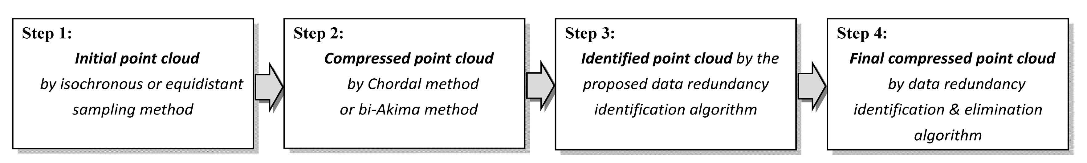
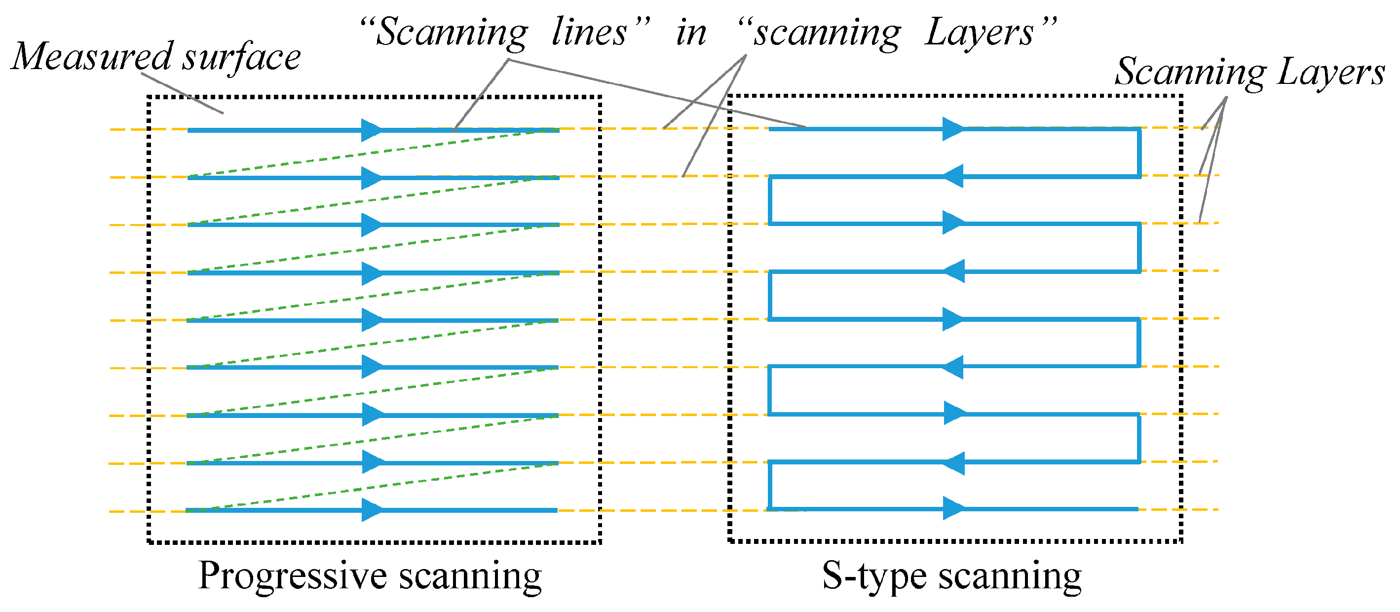
2. Innovative Methodology
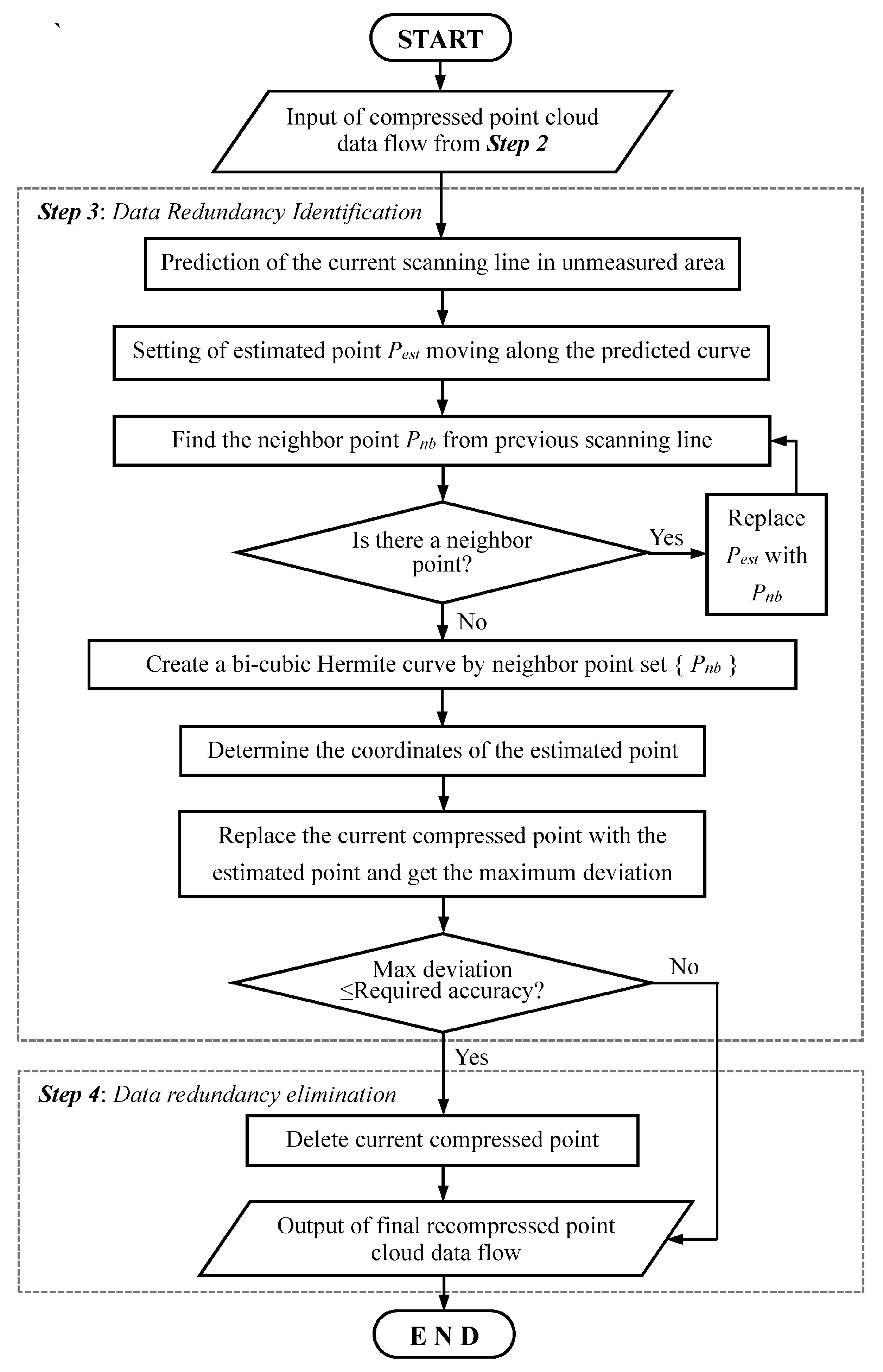
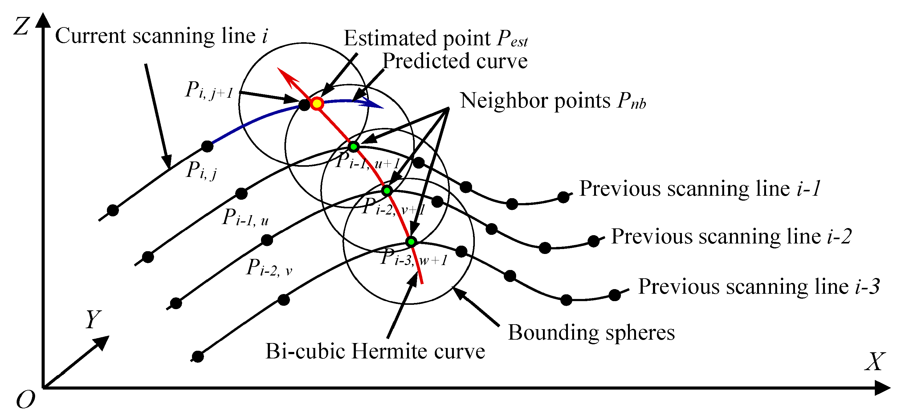
2.1. Data Redundancy Identification
2.2. Data Redundancy Elimination
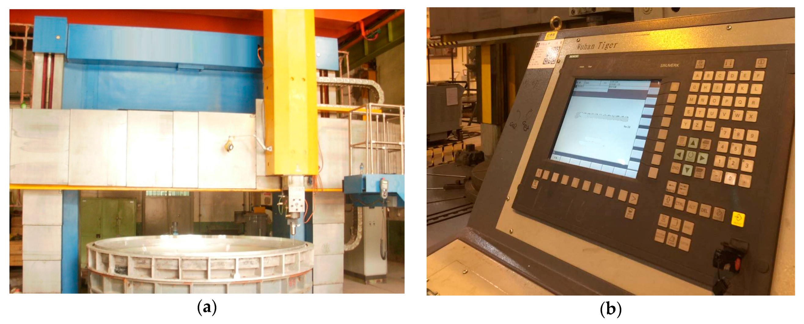
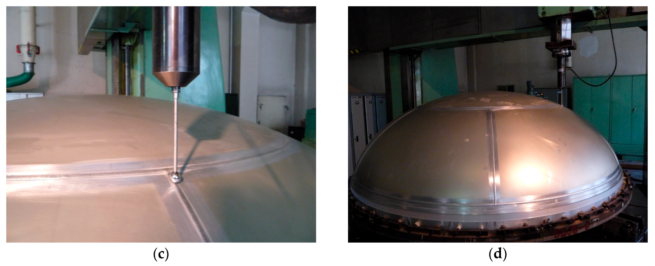
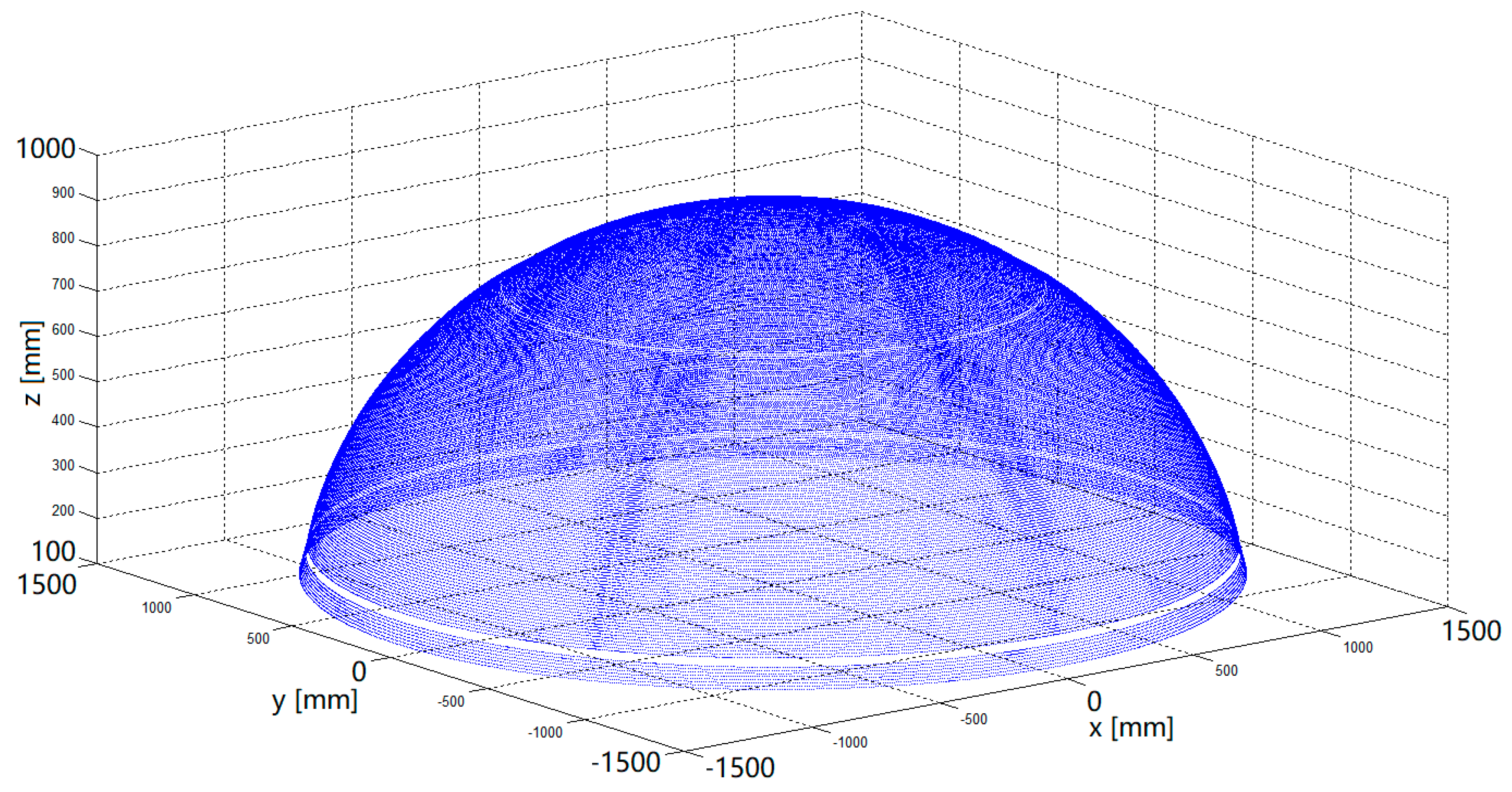
3. Experimental Results
3.1. Test A
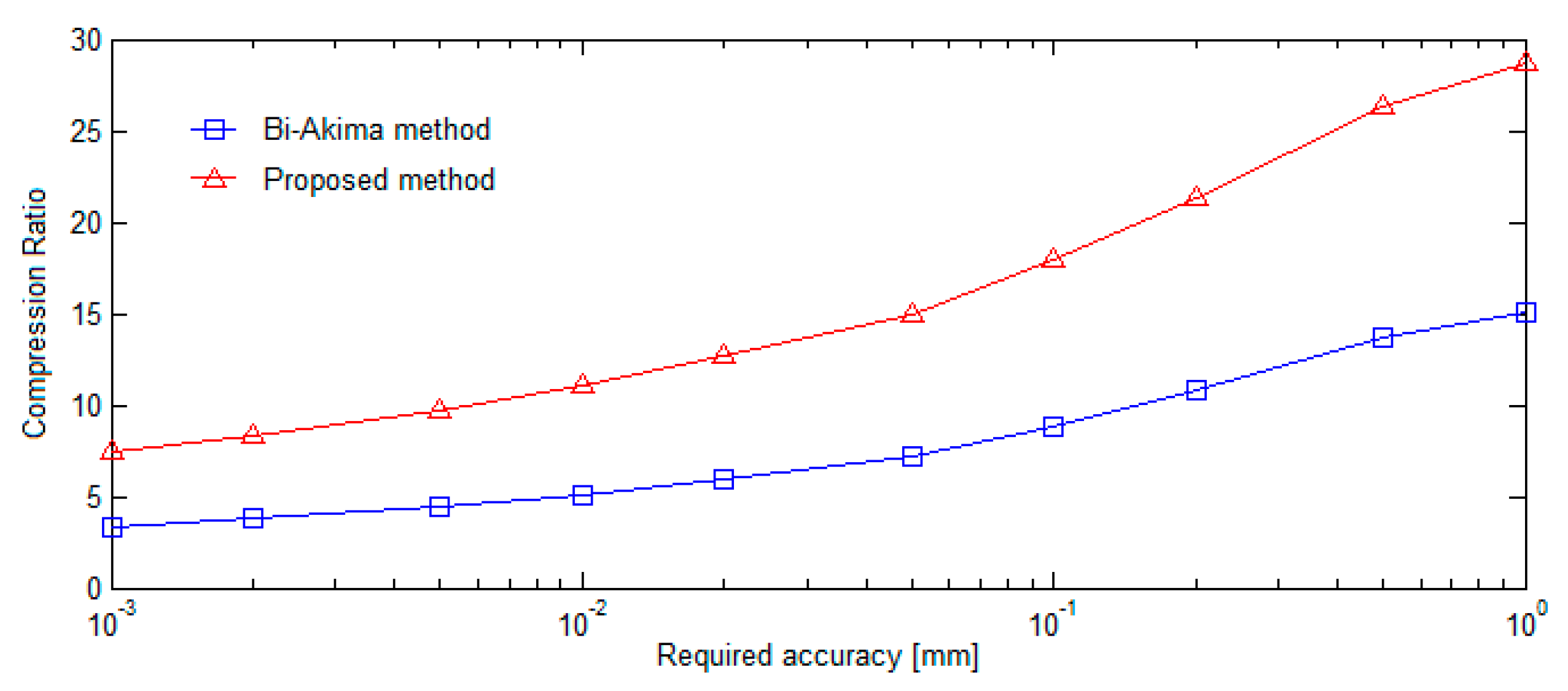
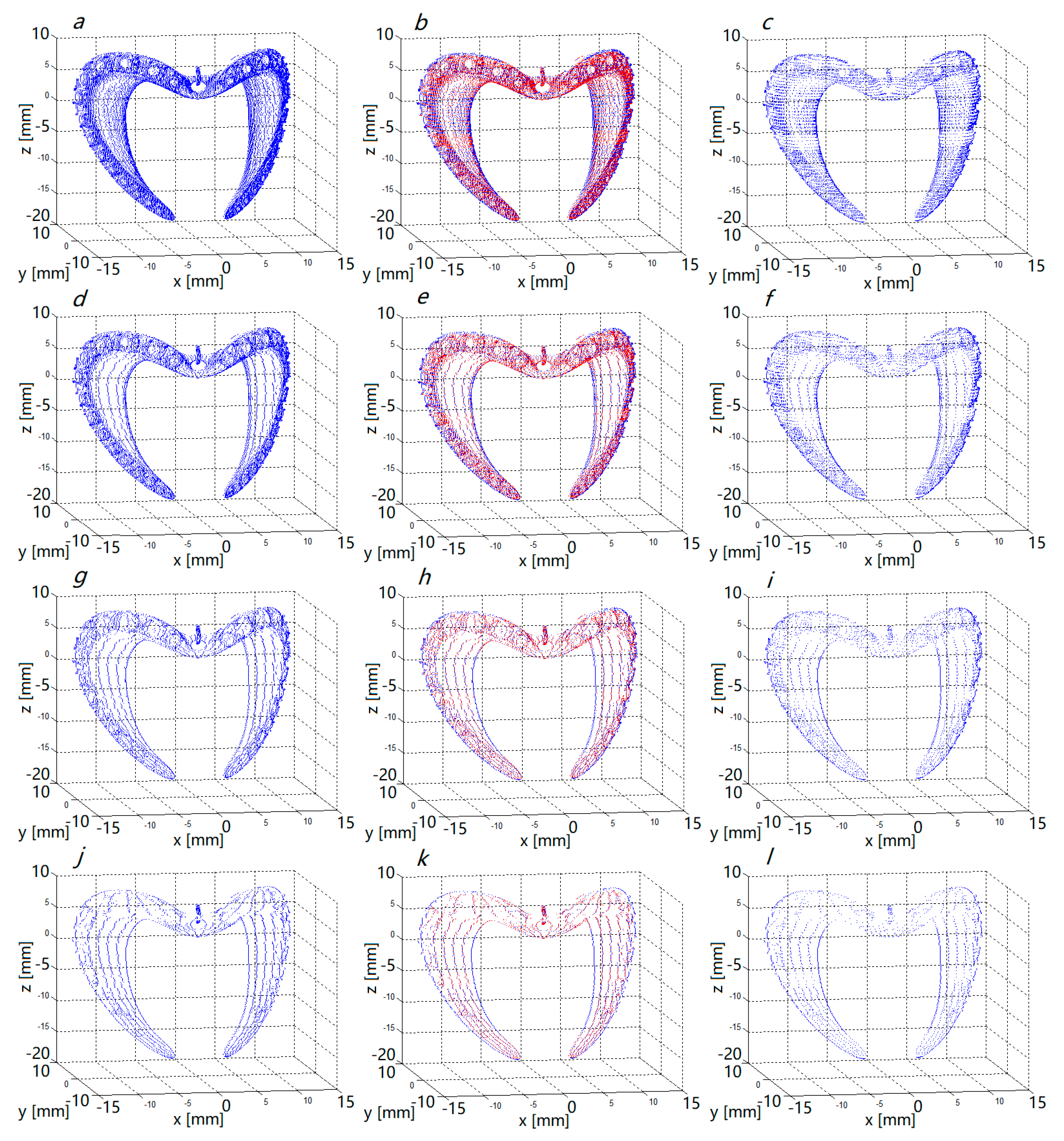
3.2. Test B
4. Discussion
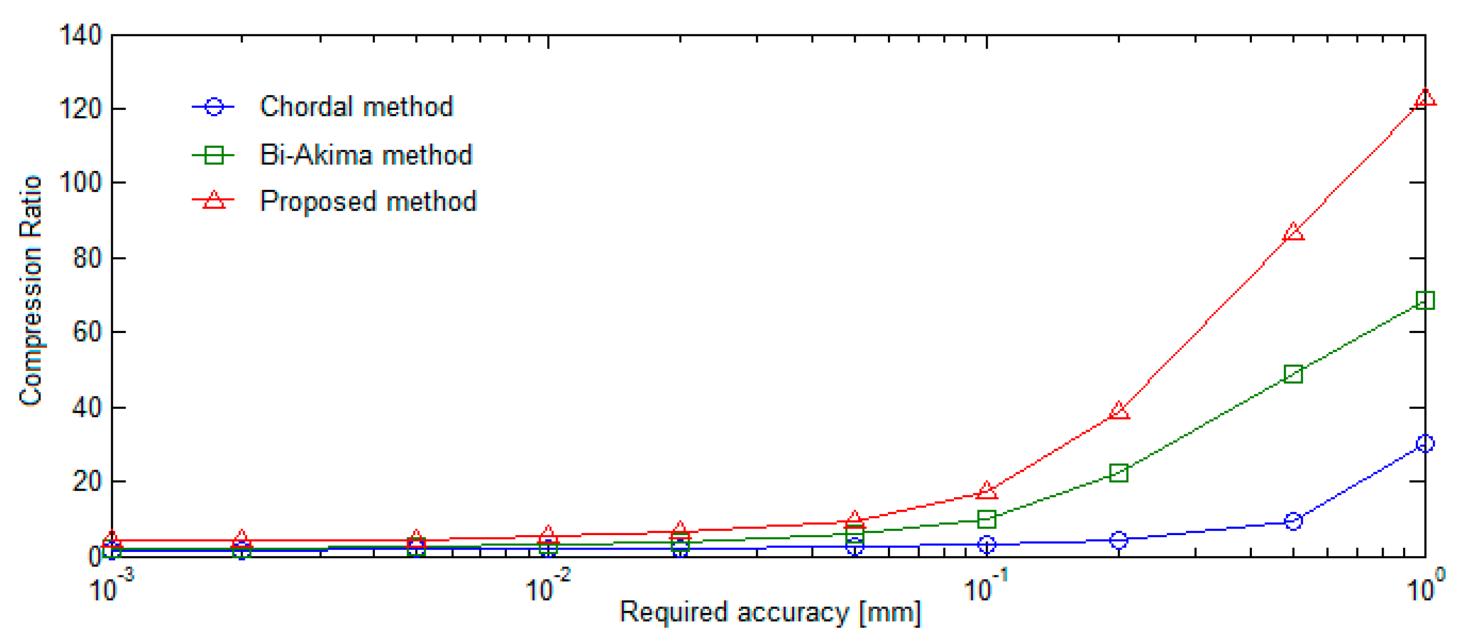
- It can further compress point cloud data and obtain a higher data compression ratio than the existing methods under the same required accuracy. Its compression performance is obviously superior to the bi-Akima and chordal methods;
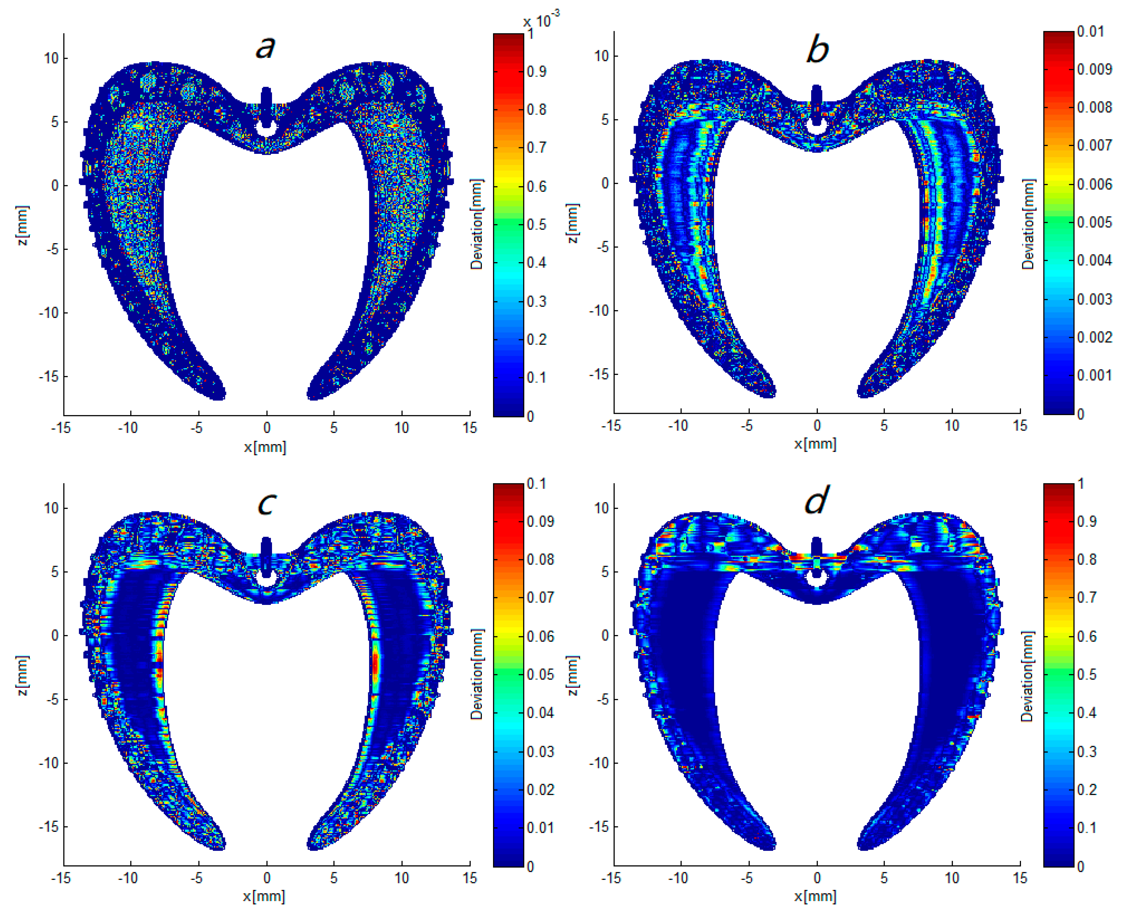
- It is capable of tightly controlling the deviation within the error tolerance range, and deviations in most measured area are far less than the required accuracy;
- Test A preliminarily verifies the application feasibility of the proposed method in an industrial environment. Test B demonstrates that the method is equally effective for complex surfaces with a large number of details, edges and sharp features, and it has stable performance;
- The proposed method has the potential to be applied to industrial environments to replace traditional on-line point cloud data compression methods (bi-Akima and chordal methods). Its potential applications may be in the real-time measurement processes of scanning devices such as contact scanning probes, laser triangle displacement sensors, mobile laser scanners, linear structured light systems, industrial CT systems, etc. The application feasibility of this method needs to be further confirmed in subsequent case studies.
- This method can only handle 3D point cloud data streams and is not suitable for processing point cloud data containing additional high-dimensional information (e.g., 3D point cloud data with grayscale or color information). We will try to solve the above problem in our future research work;
- This method can only compress the point cloud data stream which is scanned layer by layer. If the 3D point cloud is randomly sampled and there are no regular scan lines (e.g., 3D measurement with speckle-structure light), our method cannot perform effective data compression. It is a huge challenge to solve the above problems.
5. Conclusions
Author Contributions
Funding
Conflicts of Interest
References
- Galetto, M.; Vezzetti, E. Reverse engineering of free-form surfaces: A methodology for threshold definition in selective sampling. J. Mach. Tools Manuf. 2006, 46, 1079–1086. [Google Scholar] [CrossRef]
- Han, Z.H.; Wang, Y.M.; Ma, X.H.; Liu, S.G.; Zhang, X.D.; Zhang, G.X. T-spline based unifying registration procedure for free-form surface workpieces in intelligent CMM. Appl. Sci. 2017, 7, 1092. [Google Scholar] [CrossRef]
- Ngo, T.D.; Kashani, A.; Imbalzano, G.; Nguyen, K.T.Q.; Hui, D. Additive manufacturing (3D printing): A review of materials, methods, applications and challenges. Compos. Pt. B Eng. 2018, 143, 172–196. [Google Scholar] [CrossRef]
- Liu, J.; Bai, D.; Chen, L. 3-D point cloud registration algorithm based on greedy projection triangulation. Appl. Sci. 2018, 8, 1776. [Google Scholar] [CrossRef]
- Chen, L.; Jiang, Z.D.; Li, B.; Ding, J.J.; Zhang, F. Data reduction based on bi-directional point cloud slicing for reverse engineering. Key Eng. Mater. 2010, 437, 492–496. [Google Scholar] [CrossRef]
- Budak, I.; Hodolic, J.; Sokovic, M. Development of a programme system for data-point pre-processing in Reverse Engineering. J. Mater. Process. Technol. 2005, 162, 730–735. [Google Scholar] [CrossRef]
- Yan, R.J.; Wu, J.; Lee, J.Y.; Khan, A.M.; Han, C.S.; Kayacan, E.; Chen, I.M. A novel method for 3D reconstruction: Division and merging of overlapping B-spline surfaces. Comput. Aided Des. 2016, 81, 14–23. [Google Scholar] [CrossRef]
- Pal, P.; Ballav, R. Object shape reconstruction through NURBS surface interpolation. Int. J. Prod. Res. 2007, 45, 287–307. [Google Scholar] [CrossRef]
- Calì, M.; Ambu, R. Advanced 3D Photogrammetric Surface Reconstruction of Extensive Objects by UAV Camera Image Acquisition. Sensors 2018, 18, 2815. [Google Scholar] [CrossRef]
- Zanetti, E.; Aldieri, A.; Terzini, M.; Calì, M.; Franceschini, G.; Bignardi, C. Additively manufactured custom load-bearing implantable devices. Australas. Med. J. 2017, 10. [Google Scholar] [CrossRef]
- Cavas-Martinez, F.; Fernandez-Pacheco, D.G.; Canavate, F.J.F.; Velazquez-Blazquez, J.S.; Bolarin, J.M.; Alio, J.L. Study of Morpho-Geometric Variables to Improve the Diagnosis in Keratoconus with Mild Visual Limitation. Symmetry 2018, 10, 306. [Google Scholar] [CrossRef]
- Manavella, V.; Romano, F.; Garrone, F.; Terzini, M.; Bignardi, C.; Aimetti, M. A novel image processing technique for 3D volumetric analysis of severely resorbed alveolar sockets with CBCT. Minerva Stomatol. 2017, 66, 81–89. [Google Scholar] [CrossRef] [PubMed]
- Aldieri, A.; Terzini, M.; Osella, G.; Priola, A.M.; Angeli, A.; Veltri, A.; Audenino, A.L.; Bignardi, C. Osteoporotic Hip Fracture Prediction: Is T-Score-Based Criterion Enough? A Hip Structural Analysis-Based Model. J. Biomech. Eng. Trans. ASME 2018, 140, 111004. [Google Scholar] [CrossRef] [PubMed]
- Jia, Z.Y.; Lu, X.H.; Yang, J.Y. Self-learning fuzzy control of scan tracking measurement in copying manufacture. Trans. Inst. Meas. Control 2010, 32, 307–318. [Google Scholar] [CrossRef]
- Wang, Y.Q.; Tao, Y.; Nie, B.; Liu, H.B. Optimal design of motion control for scan tracking measurement: A CMAC approach. Measurement 2013, 46, 384–392. [Google Scholar] [CrossRef]
- Li, W.L.; Zhou, L.P.; Yan, S.J. A case study of blade inspection based on optical scanning method. Int. J. Prod. Res. 2015, 53, 2165–2178. [Google Scholar] [CrossRef]
- Khameneifar, F.; Feng, H.Y. Extracting sectional contours from scanned point clouds via adaptive surface projection. Int. J. Prod. Res. 2017, 55, 4466–4480. [Google Scholar] [CrossRef]
- Budak, I.; Sokovic, M.; Barisic, B. Accuracy improvement of point data reduction with sampling-based methods by Fuzzy logic-based decision-making. Measurement 2011, 44, 1188–1200. [Google Scholar] [CrossRef]
- Shi, B.Q.; Liang, J.; Liu, Q. Adaptive simplification of point cloud using k-means clustering. Comput. Aided Des. 2011, 43, 910–922. [Google Scholar] [CrossRef]
- Feng, C.; Taguchi, Y. FasTFit: A fast T-spline fitting algorithm. Comput. Aided Des. 2017, 92, 11–21. [Google Scholar] [CrossRef]
- Meng, X.L.; He, W.T.; Liu, J.Y. An investigation of the high efficiency estimation approach of the large-scale scattered point cloud normal vector. Appl. Sci. 2018, 8, 454. [Google Scholar] [CrossRef]
- Song, H.; Feng, H.Y. A progressive point cloud simplification algorithm with preserved sharp edge data. Int. J. Adv. Manuf. Technol. 2009, 45, 583–592. [Google Scholar] [CrossRef]
- Chen, L.C.; Hoang, D.C.; Lin, H.I.; Nguyen, T.H. Innovative methodology for multi-view point cloud registration in robotic 3D object scanning and reconstruction. Appl. Sci. 2016, 6, 132. [Google Scholar] [CrossRef]
- Macher, H.; Landes, T.; Grussenmeyer, P. From point clouds to building information models: 3D semi-automatic reconstruction of indoors of existing buildings. Appl. Sci. 2017, 7, 1030. [Google Scholar] [CrossRef]
- Han, H.; Han, X.; Sun, F.; Huang, C. Point cloud simplification with preserved edge based on normal vector. Optik 2015, 126, 2157–2162. [Google Scholar] [CrossRef]
- Wang, Y.Q.; Tao, Y.; Zhang, H.J.; Sun, S.S. A simple point cloud data reduction method based on Akima spline interpolation for digital copying manufacture. Int. J. Adv. Manuf. Technol. 2013, 69, 2149–2159. [Google Scholar] [CrossRef]
- Arpaia, P.; Buzio, M.; Inglese, V. A two-domain real-time algorithm for optimal data reduction: A case study on accelerator magnet measurements. Meas. Sci. Technol. 2010, 21. [Google Scholar] [CrossRef]
- Wang, D.; He, C.; Li, X.; Peng, J. Progressive point set surface compression based on planar reflective symmetry analysis. Comput. Aided Des. 2015, 58, 34–42. [Google Scholar] [CrossRef]
- Lee, K.H.; Woo, H.; Suk, T. Data reduction methods for reverse engineering. Int. J. Adv. Manuf. Technol. 2001, 17, 735–743. [Google Scholar] [CrossRef]
- Ma, X.; Cripps, R.J. Shape preserving data reduction for 3D surface points. Comput. Aided Des. 2011, 43, 902–909. [Google Scholar] [CrossRef]
- Smith, J.; Petrova, G.; Schaefer, S. Progressive encoding and compression of surfaces generated from point cloud data. Comput. Graph. 2012, 36, 341–348. [Google Scholar] [CrossRef]
- Morell, V.; Orts, S.; Cazorla, M.; Garcia-Rodriguez, J. Geometric 3D point cloud compression. Pattern Recognit. Lett. 2014, 50, 55–62. [Google Scholar] [CrossRef]
- Lu, J.C.; Yang, J.K.; Mu, L.C. Automatic tracing measurement and close data collection system of the free-form surfaces. J. Dalian Univ. Technol. 1986, 24, 55–59. (In Chinese) [Google Scholar]
- ElKott, D.F.; Veldhuis, S.C. Isoparametric line sampling for the inspection planning of sculptured surfaces. Comput. Aided Des. 2005, 37, 189–200. [Google Scholar] [CrossRef]
- Wozniak, A.; Balazinski, A.; Mayer, R. Application of fuzzy knowledge base for corrected measured point determination in coordinate metrology. In Proceedings of the Annual Meeting of the North American Fuzzy Information Processing Society, San Diego, CA, USA, 24–27 June 2007. [Google Scholar]
- Jia, Z.Y.; Lu, X.H.; Wang, W.; Yang, J.Y. Data sampling and processing for contact free-form surface scan-tracking measurement. Int. J. Adv. Manuf. Technol. 2010, 46, 237–251. [Google Scholar] [CrossRef]
- Tao, Y.; Li, Y.; Wang, Y.Q.; Ma, Y.Y. On-line point cloud data extraction algorithm for spatial scanning measurement of irregular surface in copying manufacture. Int. J. Adv. Manuf. Technol. 2016, 87, 1891–1905. [Google Scholar] [CrossRef]
- Li, R.J.; Fan, K.C.; Huang, Q.X.; Zhou, H.; Gong, E.M. A long-stroke 3D contact scanning probe for micro/nano coordinate measuring machine. Precis. Eng. 2016, 43, 220–229. [Google Scholar] [CrossRef]
- Wang, Y.Q.; Liu, H.B.; Tao, Y.; Jia, Z.Y. Influence of incident angle on distance detection accuracy of point laser probe with charge-coupled device: Prediction and calibration. Opt. Eng. 2012, 51, 083606. [Google Scholar] [CrossRef]
- Valkenburg, R.J.; McIvor, A.M. Accurate 3D measurement using a structured light system. Image Vis. Comput. 1998, 16, 99–110. [Google Scholar] [CrossRef]
- Carmignato, S. Accuracy of industrial computed tomography measurements: Experimental results from an international comparison. CIRP Ann. Manuf. Technol. 2012, 61, 491–494. [Google Scholar] [CrossRef]
- Lamberty, A.; Schimmel, H.; Pauwels, J. The study of the stability of reference materials by isochronous measurements. Anal. Bioanal. Chem. 1998, 360, 359–361. [Google Scholar] [CrossRef]
- Li, W.D.; Zhou, H.X.; Hong, W. A Hermite inter/extrapolation scheme for MoM matrices over a frequency band. IEEE Antennas Wirel. Propag. Lett. 2009, 8, 782–785. [Google Scholar] [CrossRef]


| Technical Characteristics | Values |
|---|---|
| Scope of X axis | 2400 mm |
| Positioning accuracy of X axis | 0.019 mm/1000 mm |
| Repeatability of X axis | 0.016 mm/1000 mm |
| Scope of Z axis | 1200 mm |
| Positioning accuracy of Z axis | 0.010 mm/1000 mm |
| Repeatability of Z axis | 0.003 mm/1000 mm |
| Positioning accuracy of C axis | 6.05″ |
| Repeatability of C axis | 2.22″ |
| Measuring range of scanning probe | ±1 mm |
| Accuracy of scanning probe | ±8 μm |
| Repeatability of scanning probe | ±4 μm |
| Stylus length of probe | 100 mm/150 mm/200 mm |
| Contact force (with stylus of 200 mm) | 1.6 N/mm |
| Weight of scanning probe | 1.8 kg |
| Required Accuracy (mm) | Number of Points | Compression Ratio | ||||
|---|---|---|---|---|---|---|
| Chordal Method | Bi-Akima Method | Proposed Method | Chordal Method | Bi-Akima Method | Proposed Method | |
| 0.001 | 237,363 | 122,929 | 67,448 | 1.15 | 2.22 | 4.04 |
| 0.002 | 189,824 | 120,952 | 67,121 | 1.44 | 2.25 | 4.06 |
| 0.005 | 152,674 | 110,175 | 63,813 | 1.79 | 2.47 | 4.27 |
| 0.01 | 136,027 | 93,588 | 51,062 | 2.00 | 2.91 | 5.34 |
| 0.02 | 123,891 | 71,629 | 41,862 | 2.20 | 3.81 | 6.51 |
| 0.05 | 103,205 | 44,072 | 28,837 | 2.64 | 6.19 | 9.45 |
| 0.1 | 87,008 | 27,894 | 15,974 | 3.13 | 9.77 | 17.07 |
| 0.2 | 61,124 | 12,191 | 7102 | 4.46 | 22.36 | 38.39 |
| 0.5 | 28,473 | 5594 | 3140 | 9.58 | 48.74 | 86.83 |
| 1 | 9029 | 3969 | 2217 | 30.20 | 68.69 | 122.99 |
| Required Accuracy (mm) | Number of Points | Compression Ratio | ||
|---|---|---|---|---|
| Bi-Akima Method | Proposed Method | Bi-Akima Method | Proposed Method | |
| 0.001 | 18,906 | 8516 | 3.35 | 7.44 |
| 0.002 | 16,857 | 7609 | 3.76 | 8.33 |
| 0.005 | 14,323 | 6563 | 4.42 | 9.66 |
| 0.01 | 12,432 | 5743 | 5.10 | 11.04 |
| 0.02 | 10,720 | 5007 | 5.91 | 12.66 |
| 0.05 | 8767 | 4232 | 7.23 | 14.98 |
| 0.1 | 7190 | 3535 | 8.81 | 17.93 |
| 0.2 | 5892 | 2974 | 10.76 | 21.31 |
| 0.5 | 4625 | 2412 | 13.70 | 26.28 |
| 1 | 4204 | 2213 | 15.08 | 28.64 |
© 2018 by the authors. Licensee MDPI, Basel, Switzerland. This article is an open access article distributed under the terms and conditions of the Creative Commons Attribution (CC BY) license (http://creativecommons.org/licenses/by/4.0/).
Share and Cite
Li, Y.; Ma, Y.; Tao, Y.; Hou, Z. Innovative Methodology of On-Line Point Cloud Data Compression for Free-Form Surface Scanning Measurement. Appl. Sci. 2018, 8, 2556. https://doi.org/10.3390/app8122556
Li Y, Ma Y, Tao Y, Hou Z. Innovative Methodology of On-Line Point Cloud Data Compression for Free-Form Surface Scanning Measurement. Applied Sciences. 2018; 8(12):2556. https://doi.org/10.3390/app8122556
Chicago/Turabian StyleLi, Yan, Yuyong Ma, Ye Tao, and Zhengmeng Hou. 2018. "Innovative Methodology of On-Line Point Cloud Data Compression for Free-Form Surface Scanning Measurement" Applied Sciences 8, no. 12: 2556. https://doi.org/10.3390/app8122556
APA StyleLi, Y., Ma, Y., Tao, Y., & Hou, Z. (2018). Innovative Methodology of On-Line Point Cloud Data Compression for Free-Form Surface Scanning Measurement. Applied Sciences, 8(12), 2556. https://doi.org/10.3390/app8122556