Abstract
The objective of this study was to evaluate the applicability of a flow model with different numbers of spatial dimensions in a hydraulic features solution, with parameters such a free surface profile, water depth variations, and averaged velocity evolution in a dam-break under dry and wet bed conditions with different tailwater depths. Two similar three-dimensional (3D) hydrodynamic models (Flow-3D and MIKE 3 FM) were studied in a dam-break simulation by performing a comparison with published experimental data and the one-dimensional (1D) analytical solution. The results indicate that the Flow-3D model better captures the free surface profile of wavefronts for dry and wet beds than other methods. The MIKE 3 FM model also replicated the free surface profiles well, but it underestimated them during the initial stage under wet-bed conditions. However, it provided a better approach to the measurements over time. Measured and simulated water depth variations and velocity variations demonstrate that both of the 3D models predict the dam-break flow with a reasonable estimation and a root mean square error (RMSE) lower than 0.04, while the MIKE 3 FM had a small memory footprint and the computational time of this model was 24 times faster than that of the Flow-3D. Therefore, the MIKE 3 FM model is recommended for computations involving real-life dam-break problems in large domains, leaving the Flow-3D model for fine calculations in which knowledge of the 3D flow structure is required. The 1D analytical solution was only effective for the dam-break wave propagations along the initially dry bed, and its applicability was fairly limited.
1. Introduction
A large natural hazard is posed by dam failure and ensuing potentially catastrophic floods downstream, because of the uncontrolled release of the water [1] stored in the reservoir. To mitigate this impact to the greatest possible degree, it is important to predict the dam-break wave motion by capturing both the temporal and spatial evolutions of floods to manage and reduce the risks caused by flooding [2] and to predict the propagation process effects of the dam-break waves downstream [3]. However, predicting these quantities is challenging, and selecting a suitable model to simulate the movement of the dam-break flood accurately and provide useful information on the flow field is therefore an essential step [4]. The choice of suitable mathematical and numerical models has been shown to be very significant in dam-break flood analyses.
Studies on dam-break flows as conducted in analytical solutions began more than one hundred years ago. Ritter [5] first derived the earliest analytical solution of the 1D de Saint-Venant equations over a dry bed, Dressler [6,7] and Whitham [8] studied wavefronts influenced by frictional resistance, and Stoker [9] extended Ritter’s solution to the 1D dam-break problem for a wet bed. Marshall and Méndez [10] applied the methodology developed by Godunov [11] for Euler equations of gas dynamics to devise a general procedure for solving the Riemann problem under wet bed conditions. Toro [12] conducted a complete 1D exact Riemann solver to address both wet- and dry-bed conditions. Chanson [13] studied the simple analytical solutions for floods originating from sudden dam-breaks using the characteristics method. However, these analytical solutions did not produce accurate results, particularly for wet beds during the initial stages of a dam break [14,15].
Developments from past studies have provided several numerical models aimed at solving the so-called dam break flooding problem [16], and one-dimensional models, such as Hec-Ras, DAMBRK and MIKE 11, etc. have been used to model dam-break flooding [17]. Two-dimensional (2D) depth-averaged equations have also been widely used to simulate the dam-break flow problem [18,19,20,21,22], and the results show that shallow water equations (SWE) are suitable for representing fluid flows. However, in some cases, the solutions provided by 2D numerical solvers may not be consistent with the experiments, particularly in the near field [23,24]. Furthermore, one and two-dimensional models are limited at capturing some details about three-dimensional phenomena [25]. Several three-dimensional (3D) models based on the Reynolds-averaged Navier-Stokes equations (RANS) have been applied to model dam-break flows in an effort to overcome some of the shortcomings of shallow-water models, which were employed to understand the actual behavior of complex flows during the initial stages of a dam break [26,27,28] and to study dam-break flows resulting from wave impacts on an obstacle or a bottom sill [19,29] and turbulent dam-break flow behavior in the near field [4]. Recently, among the commercially available numerical models, the well-known 3D volume of fluid method (VOF)-based CFD modelling software FLOW-3D has been used widely to analyze unsteady free surface flows, due to the increase in computing power brought about by progress in computer technology. This software calculates numerical solutions to RANS equations using a finite-difference approximation, and it also uses the VOF for tracking the free surface [30,31]; it has been used successfully to model dam-break flows [32,33].
However, there are certain hydraulic features of dam break flows over space and time that cannot be captured using 2D shallow-water models. The application of full 3D Navier-Stokes equations for real-life field-scale simulations has a higher computational cost [34], and the desired outcomes might not yield more accurate results than the shallow-water model [35]. Therefore, to evaluate both the capability of 3D models and their calculation efficiency, this paper attempts a simplified 3D model-MIKE 3 FM for simulating dam-break flows. The MIKE 3 model has been applied to investigations of several hydrodynamic simulations in natural water basins. It has been used by Bocci et al. [36], Nikolaos and Georgios [37] and Goyal and Rathod [38] for hydrodynamic simulations in field studies. Even with the considerable work of these authors, there have been very few studies on the modelling of dam-breaks using the MIKE 3 FM. In addition, research comparing the performance of 3D shallow water and fully 3D RANS models for solving the problem of dam-break flood propagation has yet to be reported. To fill this gap, the primary objective of the current study is aimed at evaluating simplified 3D SWE, detailed RANS models and analytical solutions for simulating sudden dam-break flows to analyze their accuracy and their applicability to the dam-break problem.
There is a need to validate the numerical models before attempting to perform a hydrodynamic simulation to solve real-life dam-break problems. It is an accepted practice to check numerical models using a set of experimental benchmarks. Limited measured data have been acquired in recent years, due to the difficulties of obtaining field data. This paper draws from the validation proposed by two test cases by Ozmen-Cagatay and Kocaman [30] and Khankandi et al. [39]. In the first experiment, which was conducted by Ozmen-Cagatay and Kocaman [30], there was a dam-break flood wave during the initial stage over different tailwater levels, and it provided measurements of the free surface profiles. Ozmen-Cagatay and Kocaman [30] compared only the free surface profile calculated by the numerical solutions from the 2D SWE and 3D RANS involving Flow-3D software during the initial stage. During the second experiment, which was designed by Khankandi et al. [39], measurements from this experiment were used to validate the numerical models aimed at simulating the flood propagation and providing measured data, including free surface profiles during the late stage, time evolutions of the water levels, and velocity variations. A study by Khankandi et al. [39] primarily focused on the experimental investigation, and it only mentions the water level with Ritter’s solution during the initial stage, because in a 1D analytical solution without boundary conditions (with an infinite channel length both upstream and downstream), it makes no sense to compare the experimental results with the Ritter (dry bed) or Stoker (wet bed) solutions when the reflections from the walls affected the depth profiles, and when further comparisons with numerical simulations for the experiments in Reference [39] are poor. In aiming directly at these problems, this paper will present a full comparative study on free surface profiles, water depth variations and velocity variations during the entire dam-break process. Here, numerical simulations of the dam break wave are developed using two 3D models for an instantaneous dam break in a finite reservoir with a rectangular channel that is initially dry and wet.
This paper is organized as follows: The governing equations for the two models are first introduced before the numerical scheme is described. The typical simplified test cases were simulated using 3D numerical models and a 1D analytical solution. The model results and the ways in which they compare with the laboratory experiments are discussed, and simulated results of the variations in hydraulic elements over time at different water depth ratios are presented before the conclusions are drawn.
2. Materials and Methods
2.1. Data
First, measurements of free surface profiles during the initial dam-break stages over horizontal dry and wet beds were conducted by Ozmen-Cagatay and Kocaman [30]. During this test, the smooth and rectangular horizontal channel was 0.30 m wide, 0.30 m high, and 8.9 m long, as illustrated in Figure 1. The channel was separated by the vertical plate (dam) located 4.65 m from the channel entrance; that is, the lengths of the reservoir, , and the downstream channel, . The reservoir was located on the left side of the dam and was initially considered inundated; the initial upstream water depth h0 in the reservoir was constant at 0.25 m. On the right side, the initial tailwater depths were 0 m in the case of the dry bed and 0.025 and 0.1 m in the wet bed, so there were three different situations with water depth ratios of 0, 0.1, and 0.4. The wet-bed conditions were created by using a low weir at the end of a flume. The water surface profiles were observed at the early stage using three high-speed digital cameras (50 frames/s), and the accuracy of the instrumental measurements was demonstrated in Reference [30]. In the following section, the corresponding numerical results refer to positions x = −1 m (P1), −0.5 m (P2), −0.2 m (P3), +0.2 m (P4), +0.5 m (P5), +1 m (P6), +2 m (P7), and +2.85 m (P8), where the origin of the coordinate system x = 0 is at the dam site. The three water depth ratios of 0, 0.1, and 0.4, where the coordinates are normalized by
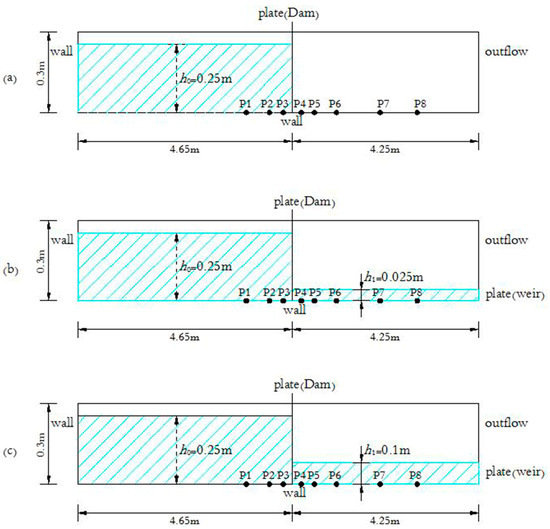
Figure 1.
Schematic view of the experimental conditions by Ozmen-Cagatay and Kocaman [30]: (a) α = 0; (b) α = 0.1; and (c) α = 0.4.
Both models are then tested against experimental data designed by Khankandi et al. [39]. The measurements, taken during the experiment, make up a dataset that can be used for numerical model validation for problems involving free surface profiles during late stages, water depth variations, and averaged velocity evolutions. The Perspex flume was rectangular from the top and horizontal views, as shown in Figure 2, with a Manning coefficient of 0.011. It was 0.51 m wide, 0.50 m high and 12.80 m long. The upstream initial water depth was 0.40 m and the length of the reservoir, , was 3.50 m. The initial tailwater depths were 0 m for the dry-bed condition and 0.08 m for the wet-bed condition (i.e., of 0 and 0.20). During this test, a high-speed digital camera was used to obtain the measured continuous water surface profiles, and the corresponding water level variations and average velocity variations in different positions were measured for the dry-bed and wet-bed conditions using ultrasonic sensors and ADV, respectively. In the following figure, the measured and computed stage-time hydrographs and velocity variations refer to positions x = −0.5 m (G1), −0.1 m (G2), +0.1 m (G3), +0.8 m (G4), +1.0 m (G5), +1.2 m (G6), +3.0 (G7) and +5.5 m (G8) (see Figure 2).
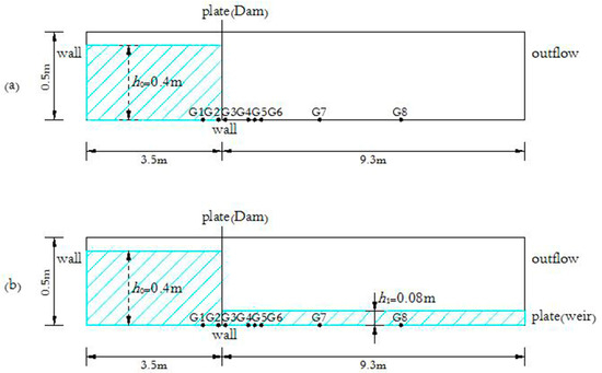
Figure 2.
Schematic view of the experimental conditions by Khankandi et al. [39]: (a) α = 0 and (b) α = 0.2.
2.2. Model Performance Criteria
The accuracy of the modelling results can be quantified by using the statistical variable root-mean-square error (RMSE), which is defined as follows:
where N is the number of samples and and are the measured and calculated values, respectively. The best fit between the experimental and predicted values would have an RMSE = 0.
2.3. Analytical Solution
The 1D Ritter’s analytical solution [5] for an idealized instantaneous dam failure under dry frictionless downstream-bed conditions is
where is the water surface elevation, is the initial water depth, is the velocity in the x-direction and is time.
The analytical case of a wet bed (non-zero depth downstream ) downstream at a depth involves the initial condition and a bore travelling downstream into the still water region, as shown in Figure 3, where the dam-break flow regimes are divided into four zones by Stoker [9]. The upstream region of wave propagation is
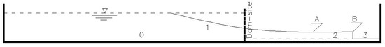
Figure 3.
Typical profiles of the dam-break flow regimes for Stoker’s analytical solution [9]: Wet-bed downstream.
A physical constraint defining the bore is that the velocity is continuous at the boundary between regions 1 and 2 where the elevation is also continuous. At this boundary (A) from region 1
where , and is thus the value for region 2. A constant mass flux must also be maintained across the bore (position B) advancing with speed , giving
where and , and with the equation for a bore moving into still water of
The situation is defined and may be solved through an iterative procedure. Substituting for and gives , which is independent of time.
2.4. Numerical Model and Simulation Setup
2.4.1. Flow-3D
Flow-3D is a commercially available computational fluid dynamics (CFD) software package that is commonly used to model hydraulic structures, such as drainage culverts, spillways, and stilling basins. It calculates numerical solutions to RANS equations using a finite-difference approximation, and it also uses the volume of fluid (VOF) method for tracking the free surface. The solid geometry is represented using a cell porosity technique called the FAVOR method [40]. The governing continuity and RANS equations in Flow-3D for Newtonian, incompressible fluid flow are:
where = velocity component in the i, j direction, = fractional area open to flow in the i, j direction, = time, = volume fraction of fluid in each cell, = fluid density, = pressure, = gravitational force in the i direction, and = the diffusion transport term. In the present study, the equations for the motion are closed with the standard model for turbulence closure, k is the turbulence kinetic energy, and is the turbulent dissipation rate, and they were modelled in the dam-break problem application. The model for turbulence closure is used to determine the turbulent viscosity to perform a simulation for the present two cases.
Simulation Setup of Experiments by Ozmen-Cagatay and Kocaman [30]
For the Flow-3D model, the RANS solution domain is 8.90 m in length, 0.30 m in width, and 0.30 m in height. The simulations are also conducted with coarser and finer meshes consisting of fixed rectangular cells measuring 2 mm, 5 mm, 10 mm and 20 mm. The corresponding total cells of the mesh system are 667,500, 106,800, 26,700, and 6675. Figure 4 illustrates the differences between the simulated and measured free surface profile for different mesh sizes. Considering a wet bed case of , an index of the root mean square error (RMSE) is calculated and presented. The computational time for the simulations at four mesh sizes is also shown in Figure 4. The simulated results are convergent under four grid sizes; only insignificant differences in the statistical variable RMSE are observed, but the computational efforts are quite different. Therefore, regarding both the accuracy and the computational cost, the grid spacing is set to m. The upstream and lower boundaries are set as a wall, due to a lack of inflow. The downstream boundary is set as outflow for the dry-bed condition and as a wall for the wet-bed condition. The upper and channel sidewall boundaries are set as symmetrical.
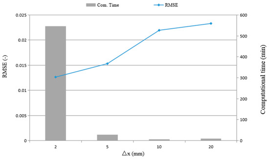
Figure 4.
Sensitivity analysis of the numerical simulation using Flow-3D for the different mesh sizes of the experiments in Reference [30].
Simulation Setup of Experiments by Khankandi et al. [39]
For the Flow-3D model, the computational domain is discretized into rectangular cells that are 0.005 m long and 0.005 m high. The mesh system consists of 256,000 total cells. The settings of the boundaries are same as they are in Ozmen-Cagatay and Kocaman [30].
2.4.2. MIKE 3 FM
The MIKE 3 flow model FM is a modelling system based on a flexible mesh (FM) approach developed at the Danish Hydraulic Institute (DHI), and it is based on a finite volume, unstructured mesh approach. The flexible mesh is most suitable for irregular water body boundaries. The MIKE 3 FM is based on the numerical solution of the 3D incompressible RANS equations when subject to the Boussinesq approximation and an assumption of hydrostatic pressure. The continuity equation and horizontal momentum equations [41] can be written as
where , , and are the Cartesian coordinates, and , , and are the velocity components along the x, y, and z directions, respectively; is the magnitude of the discharge from point sources, and and are the velocities at which the water is discharged into the ambient water; is the surface elevation; is the still water depth; is the total water depth; is the Coriolis parameter; is the gravitational acceleration; is the density of water, and is the reference density of water; , , , and are components of the radiation stress tensor; is the atmospheric pressure; is the vertical turbulent (or eddy) viscosity; and and are the horizontal stress terms.
In the MIKE 3 FM model, the free surface is taken into account using a sigma-coordinate transformation approach. Discretization in the solution domain is performed using a finite volume method. Spatial discretization of the primitive equations is performed using a cell-centered finite volume method. In the horizontal plane, an unstructured grid is used while in the vertical direction, the discretization is structured [41]. The Coriolis and wind force are neglected for small scale physical model in present work.
Simulation Setup of Experiments by Ozmen-Cagatay and Kocaman [30]
For the MIKE 3 FM model, the simulations are conducted with mesh resolutions of 0.15, 0.1, 0.05, and 0.01 m corresponding to 120, 267, 1068, and 26,700 elements; the results of the mesh sensitivity analysis for all the grids are shown in Figure 5, indicating that the grid size of 0.05 m is suitable for the purpose of this study. A suitable grid size and time step lead to better fitting and predicted precision and a faster convergence speed. In the subsequent numerical computations, uniform grid systems with a minimum guide spacing of 0.05 m, the time step of 0.01 s and 4000 time steps are applied so that the Courant-Friedrich-Levy (CFL) condition is sufficient to guarantee stability and satisfactory accuracy for the model. The eddy viscosity is determined using Smagorinsky’s formulation in the horizontal direction and the standard model in the vertical direction. The upstream and lateral boundaries of the domain are set as the land boundary so that no water flows into the reservoir; the reservoir length is held constant, the downstream boundaries are set as free outlets, and a downstream far-field boundary condition [42] is adopted in the dry-bed case. The weir in the downstream boundary is set for the wet bed. The initial condition is defined as specified constant level in the upstream reservoir and tailwater water depth in the downstream area. Manning coefficient n used in the numerical computation is given the constant value of 0.012, which corresponds to the tested Perspex flume.
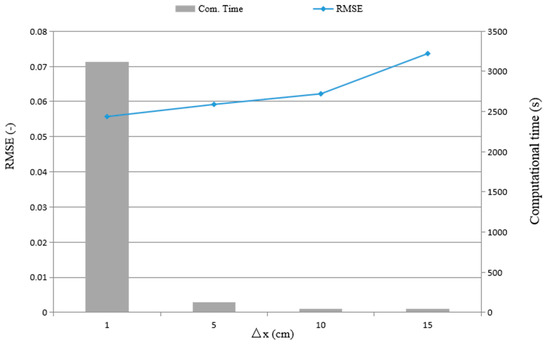
Figure 5.
Sensitivity analysis of the numerical simulation using MIKE 3 FM for the different mesh sizes of the experiments in Reference [30].
Simulation Setup of Experiments by Khankandi et al. [39]
For the MIKE 3 FM model, simulations were conducted with mesh resolutions of 0.2, 0.1, 0.05, and 0.01 m, with mesh independence occurring at 0.05 m. The results presented here are derived from computations using the 0.05 m mesh, which had approximately 3132 nodes and 2860 quadrilateral elements. A fixed time step of 0.001 s was applied over 30,000 times. In the numerical computations, the eddy viscosity and upstream boundary had the same settings as those for previous experiments for the dry-bed case, except for the use of a constant water level at downstream boundaries for the wet-bed case. The value of Manning coefficient n was set to 0.011, which corresponds to the tested Perspex flume configuration.
3. Comparison between Flow-3D, MIKE 3 FM, and 1D Exact Riemann Solver Predictions
3.1. Free Surface
3.1.1. Free Surface during the Early Stage
Figure 6, Figure 7 and Figure 8 show a comparison of free-surface profiles during the early stage along a wall of the testing flume [30] at different times using dry- and wet-bed conditions downstream. The figures also present free surface profiles with a 1D Ritter’s analytical solution [5], which would serve as a means to check the accuracy and robustness of the simulated results in the numerical model. In all the free-surface profiles in Figure 6, Figure 7, Figure 8 and Figure 9, the water depths () and horizontal distances () were transferred into dimensionless parameters with the initial water depth . An error analysis of the free-surface profile results obtained by the 1D analytical results and Flow-3D and MIKE 3 FM models are summarized in Table 1.
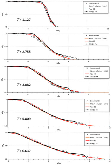
Figure 6.
Comparison between observed and simulated free surface profiles at dimensionless times T = t(g/h0)1/2 and for dry-bed (). The experimental data are from Reference [30].
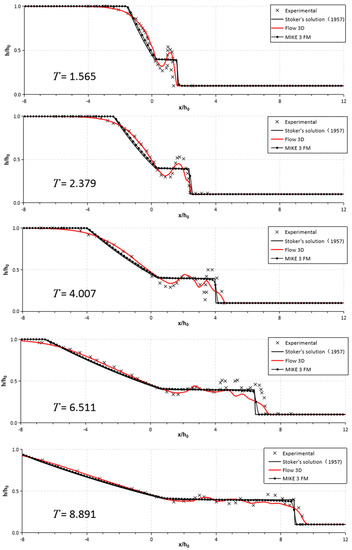
Figure 7.
Comparison between observed and simulated free surface profiles at dimensionless times T = t(g/h0)1/2 and for a wet-bed (α = 0.1). The experimental data are from Reference [30].
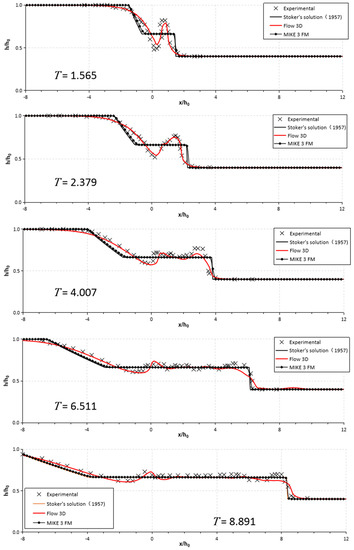
Figure 8.
Comparison between observed and simulated free surface profiles at dimensionless times T = t(g/h0)1/2 and for the wet-bed (α = 0.4). The experimental data are from Reference [30].
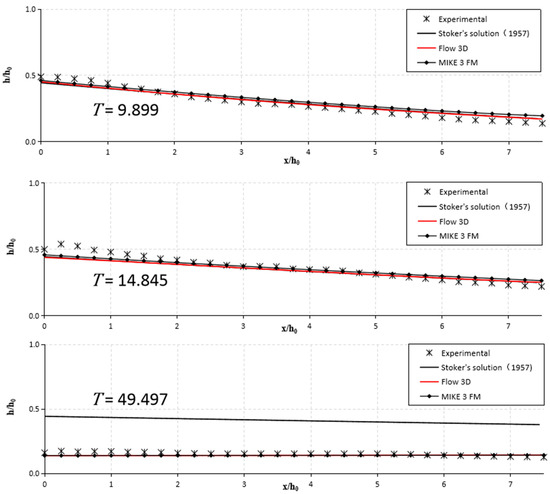
Figure 9.
Experimental and numerical comparison of free surface profiles during late stages at various dimensionless times T after the failure in the dry-bed by Khankandi et al. [39].

Table 1.
RMSE values for the free surface profiles observed by Ozmen-Cagatay and Kocaman [30].
Good consistency was found between the RANS results obtained by Flow-3D and measurements for the dry-bed test (), as shown in Figure 6. The surface profiles were originally parabolic and the wavefront became convex as time progressed. However, the 3D SWE results obtained by MIKE 3 FM and the 1D analytical results of Ritter’s solution showed small deviations from the measurements, favoring the less obvious convex solution, especially at the early initial stage. The experimental profiles after the dimensionless time were close to those computed by all three models, with T = t(g/h0)1/2. The simulated wavefront in the downstream region () using MIKE 3 FM moved more slowly than the measurements and the results of Flow-3D, indicating that the wavefront in the upstream reservoir () moved faster than the measurements and the other results. It was observed that the two numerical models and analytical solution generally had low values for the RMSE, with all of them below 0.08 at different times, which indicates that both types of solutions achieved acceptable results for the dry-bed case during the initial stage, while the Flow-3D model obtained the best RMSE result of 0.02 (Table 1). Significantly, as time passed, the error decreased from T = 1.127–6.637; the Flow-3D, MIKE 3FM, and 1D approaches improved the forecast by reducing the RMSE values by ~42.29%, ~22.87%, and ~54.84%, respectively, demonstrating that the differences between the values predicted by the three models to solve dam-break flows for dry beds were very small over time. Therefore, any of the three models can be selected as an appropriate model for predicting the free surface after the dam break for the dry-bed.
Figure 7 shows the surface profiles with a depth ratio of ; in contrast to the observation of the dry-bed case, a jet was formed by the collision between moving and still water. A jet was observed after the dam break during the initial stage in Stansby et al. [15]. The formation of a wave-like vertical jet propagating downstream for the MIKE 3 FM was quite noticeable, which was consistent with the mushroom-jet results for the RANS (Flow-3D) calculations and experiments. The difference in wave shape, especially during the early stages (T = 1.565–6.511), were attributed to the MIKE 3 FM and 1D analytical solution, and they were generally within 0.07 to 0.1 in the RMSE values, decreasing to 0.05 at T = 8.891 (Table 1). The reason for the more apparent difference between these two models and Flow-3D primarily lies in the assumption of a hydrostatic pressure distribution and the negligible vertical acceleration [30]. Despite significant deviations among the MIKE 3 FM simulation, analytical solution, and the experiments at the downstream wavefront, these two models successfully predicted the flow features after wave breaking (Figure 7). Although the differences between the calculated results compared with those of the experiments decreased when , the error was reduced. Among the three models, the Flow-3D had the best performance with the lowest RMSE, with a reduction to 0.04 from 0.09, which indicated that the estimation quality of the Flow-3D model was better than that of the MIKE 3 FM and 1D analytical solution for predicting the free surface during the initial stage in a wet bed with a depth ratio of .
Figure 8 shows a comparison of the water surface profiles in the wet-bed condition with ; the wavefront profiles during the initial stage were similar to those observed at the wet-bed case . The enlargements shown in Figure 8 for T = 1.565 and 2.379 show the mushroom-jet formation. The RANS results obtained by Flow-3D nearly coincided with the experimental data at different times, and the RMSE values were <0.06. There were similar problems at the early stages at for the 3D SWE (MIKE 3 FM) and the analytical results. Specifically, there was poor consistency with the measured results, particularly at early times after the dam break, but the differences between the MIKE 3 FM, analytical solution and flow depth measurements for this case behaved more gently than at the water depth ratio . The error analysis in Table 1 also shows smaller RMSE values than in the last case; the RMSE of the simulated free surface at T = 1.565–8.891 for the MIKE 3 FM ranged from 0.09 to 0.03 and that for the 1D analytical solution was from 0.09 to 0.04, but the error was generally reduced when . Thus, these results show that deviations decrease in the graphs when the depth ratios () increase.
To summarize, Figure 6, Figure 7 and Figure 8 depict the evolution of the free surface profiles after the dam breach. The consistency between the analytical solution and the MIKE 3 FM results was satisfactory for the dry-bed tests, but there was quite a noticeable difference in the formation of a wavefront propagating downstream for the wet-bed cases. In both the dry- and wet-bed cases, the measured profiles were very close to the corresponding ones calculated using the Flow-3D model. The comparisons demonstrated that the Flow-3D model gave more accurate results than the numerical results calculated using MIKE 3 FM. A horizontal jet formed occasionally for the dry-bed case, and a mushroom-like jet occurred for the wet-bed case, which had also been observed previously by Stansby et al. [15]. According to Quecedo et al. [28], the hydrostatic assumption does not hold for the initial instants of dam-break wave propagation from the evolution of the pressure. For wet-bed cases, the pressure variation over time was similar in the RANS (Flow-3D) calculations and in the experiments, resulting in a curved surface profile (see Figure 3 and Figure 4), but for the MIKE 3 FM and analytical solutions with a hydrostatic distribution assumption, there is a bore (i.e., a rectangular jump). Applying the three models to the dam-break flow during the initial stage offered good results, while the Flow-3D model was more realistic and demonstrated greater consistency than either the MIKE 3 FM or the 1D approach.
3.1.2. Free Surface during the Late Stage ()
To further study the free-surface profile features during the late stage () after the dam break, the experimental setup by Khankandi et al. [39] was used to compare the results computed by the two numerical models (Flow-3D and MIKE 3 FM) and the analytical solution of Stoker’s solution [9] over a longer time in the wet-bed. The experimental and computed water surface levels for the dry-bed condition are presented here. The differences in the free-surface profile when using Flow-3D and MIKE 3 FM models decreased very well with respect to one another, especially in the simulated results, and the discrepancies in the wavefront location also became slight (Figure 9). The RMSE results in Table 2 also show that the Flow-3D model offered a similar performance to that of MIKE 3 FM, with 0.02 as the minimum and 0.04 as the maximum value. However, as seen, the experimental curves and simulated curves deviated from the corresponding exact curves for T = 49.497, with the RMSE values for the 1D analytical solution reaching 0.26, the worst performance of all the models. This is because the 1D analytical Ritter (dry bed) or Stoker (wet bed) solutions are only applicable to the dam-break flow in an infinite length for both an upstream reservoir and downstream, with the consequence being that the water surface along the channel is constant over time, but it does not produce the reflections from the walls in a way that affects the depth profiles. This outcome indicates that no reflected negative wave is expected, and the reservoir will never empty [43]. Either the Flow-3D or the MIKE 3 FM model can be selected as an appropriate model for predicting the free surface during the late stage after the dam break. These behaviors illustrate that, as time passes, the MIKE 3 FM successfully predicted the flow features after dam failure like the RANS method (Flow-3D). The only exception to this success was during the initial and late stages, because the vertical velocity became progressively minor compared to the horizontal velocity while the shallow-water assumptions became more realistic.
Table 2.
RMSE values for the free surface profiles observed by Khankandi et al. [39].
3.2. Water Depth Variations
The evolution of the initial reservoir water levels of under the dry- and wet-bed conditions from Khankandi et al. [39] are shown in Figure 10 and Figure 11, respectively. Figure 10 shows the water level variations at different gauges, including upstream and downstream of the gate; there is satisfactory consistency between the experimental data and the numerical results. Positions G1 and G2 represent the water level variations in the reservoir, and they displayed a progressive reduction in the water depth variation. It was also observed that the sudden upstream water depth reduction resulted in a flow depth of ~4/9 of the initial water depth, which the expected analytical result was first presented by Ritter [5]. According to Liu et al. [44], the water level curve of the analytical solution was separated from the experimental curve from t = 3 s. Thus, for t ≥ 3 s, the analytical solution approached the constant value of the water depth of 4/9, while the experimental data decreased gradually owing to reservoir depletion. The reduction in the water depth was slow at G1 and G2, at approximately t = 1–5 s when the downstream water began to enter the reservoir backwater. A sharp variation of the water level immediately downstream of the dam behaved similarly, and it involved a decrease in the maximum water level at locations G3, G4, G6, and G8. As expected, the water level increased for t < 3 s and then exhibited an identical reduction. The RMSE values for Flow-3D and MIKE 3 FM are quite satisfactory (Table 3), with the maximum RMSE for Flow-3D being 0.03 and that of MIKE 3 FM being 0.04.
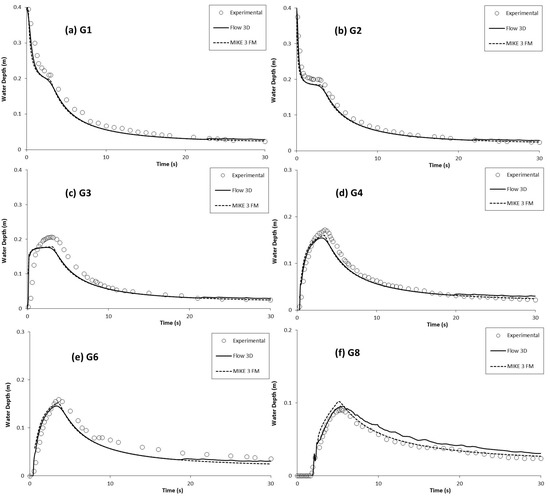
Figure 10.
Measured and computed water level hydrograph at various positions for dry-bed by Khankandi et al. [39]: (a) G1 (−0.5 m); (b) G2 (−0.1 m); (c) G3 (0.1 m); (d) G4 (0.8 m); (e) G6 (1.2 m); (f) G8 (5.5 m).
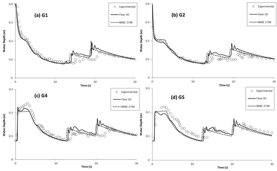
Figure 11.
Measured and computed water level hydrographs at various positions for the wet-bed by Khankandi et al. [39]: (a) G1 (−0.5 m); (b) G2 (−0.1 m); (c) G4 (0.8 m); and (d) G5 (1.0 m).
Table 3.
RMSE values for the water depth variations observed by Khankandi et al. [39] at the late stage.
Figure 11 shows the evolution of the water level with time for the wet-bed case with a tailwater level of ; that is, . Upstream and downstream for the wet-bed, the physical downgrade of the water depth was strongly interrupted by the reflected wave at the downstream end of the testing flume (as seen in Figure 11). At points G1 and G2 in the reservoir, no obvious difference was found in the variation of the water level until approximately t = 15 s, because of the wave reflected against the downstream weir. For points G4 and G5, at t < 15 s, the reflected waves became visible. When they struck the weir, they were partially reflected, and these reflected waves moved the upstream boundary, yielding the aforementioned water depth results. The simulated results using MIKE 3 FM and Flow-3D appeared to have a quicker velocity of propagation than the measurement when the wave was reflected at approximately t > 15 s. This slight delay in the measured data can be attributed to the fact that the actual opening of the gate was not instantaneous. Figure 11 also demonstrates that the numerical results are reasonably consistent with the experimental data for the propagation speed of the wavefront and the water depth variation. The water level obtained with the two numerical models decreased more rapidly than in the experiments. Moreover, the wavefront in the numerical simulation was propagated sooner than the experimental results. It can be clearly observed from Table 3 that the Flow-3D and MIKE 3 FM models had a minimal amount of error, at 0.04 and 0.03, respectively. The performances of the Flow-3D and MIKE 3 FM models for the water depth variations in the dry and wet-beds were satisfactory.
3.3. Velocity
3.3.1. Averaged Velocity Evolution
Figure 12 shows the temporal variation in velocity in the x direction at points G4 and G6 for the dry-bed case in Khankandi et al. [39]; there are notable differences at all times. The overall trends in the velocity variations between the numerical results and the measurements were similar at these two locations, decreasing after the peak value. However, a time lag and a difference in the peak velocity magnitude were observed between the simulated and measured velocity at these two locations. The simulations showed a faster rise and a higher magnitude of peak velocity compared to those of the measurements. Also note that after the peak value, the velocity of all the measurements was less than that for the simulated results of the numerical models. Again, the decrease in the measurements was faster than that for the simulated results. The reason why the calculated results overestimated the measured velocity was likely due to the initial condition; in the simulation, the gate opened instantaneously, while it took a finite amount of time for the gate to open and the flow to start in the experiment [45]. Nevertheless, in Figure 12, there were very slight differences between the velocity profiles of the Flow 3D and MIKE 3 FM results compared to those of the numerical simulation and measurements, with RMSE values of 0.26 and 0.29 at points G4 and G6 for Flow 3D and 0.23 and 0.26 for MIKE 3 FM (Table 4), indicating that there was not much deviation between the two models.
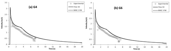
Figure 12.
Average velocity for the dry-bed at G4 (0.8 m) and G6 (1.2 m) by Khankandi et al. [39].
Table 4.
RMSE values for the averaged velocity evolution at G4 and G6 based on experimental data by Khankandi et al. [39].
3.3.2. Vertical Velocity Profiles
Figure 13 shows the streamwise (u) velocity profiles in Ozmen-Cagatay and Kocaman [39] for locations P1, P3, P5, and P6 at t = 0.8, 2, and 5 s. The magnitude of velocity simulated by the Flow-3D and MIKE 3 FM models shows a similar trend. The difference in the predicted velocity profiles highlights the computational cost of predicting the highly transient flow. It was clear that strong vertical velocity components were present in the front and on the top of the wave, resulting from the sudden change in the boundary condition. The reason for the difference in the magnitude of the velocity near the bottom of the channel was likely the different vertical spatial resolution used in the MIKE 3 FM and Flow 3D; when the water depth is larger than 0.02 m, the velocity reaches its maximum value and then does not change with the increased water depth. The results show different magnitudes of the velocities simulated by the MIKE 3 FM and Flow-3D models at both locations in the initial stage; however, in the later stage, their difference decreased, meaning that the longwave approximation became more reasonable. Further upstream and downstream of the gate, the water surface slopes were small (i.e., the u is small). At position P1, this velocity component reached a value of ~0.2 m s−1 at t = 0.8 s, indicating that the slope of the water surface sharply changed with a large u near the gate during the initial stage. The results clearly indicate that 3D effects are important in dam-break flows, and the comparisons demonstrate that the Flow-3D and MIKE 3 FM models could provide more detailed information, such as vertical velocity variations, than the 1D and 2D shallow-water models.
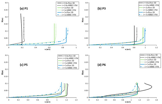
Figure 13.
Comparison of simulated velocity profiles at various locations upstream and downstream of the dam at t = 0.8 s, 2 s, and 5 s for water depth ratios α = 0.1 by Ozmen-Cagatay and Kocaman [30]: (a) P1(−1 m); (b) P3 (+0.2 m); (c) P5 (+1 m); and (d) P6 (+2 m).
3.4. Computational Costs
The validity of the 1D and 2D Shallow Water equation are compared with a known analytical solution or experimental data, which has been performed by many other researchers (see for instance [27,46]), and in the study about applying 3D models to simulate near-field dam-break flows in References [3,47]. All these comparisons showed that full 3D RANS models performed better than the 1D and 2D models, but the expensive computational effort of the 3D RANS models cannot be neglected.
A comparison of the required computational time and the number of grids was made for the simulations. The MIKE 3 FM model has considerably lower computational costs, and it was 24 times faster than the Flow-3D in all cases (Table 5). All of the numerical simulations were performed using an Intel® Core™ i5 PC. The comparison between the simulated and experimental results, as showed for the first test case in Ozmen-Cagatay and Kocaman [30], clearly shows that the 3D RANS approach has the ability to represent the water surface profiles quite well during the entire dam-break process, immediately during the initial stage and after the gate collapse, and it reproduced the free-surface profiles of the front wave well for dry- and wet-bed conditions while the wave-front modelled by the MIKE 3 FM model for the wet-bed case was a rectangular jump rather than a curved surface. For the dam-break flow under a dry bed, the results of the free surface profiles during the late stage using the MIKE 3 FM approach can be considered reasonable relative to the experimental measurements. The performances of the MIKE 3 FM models in relation to the water depth variations and velocity variation for the dry- and wet-beds were satisfactory. The previous research results show the practical advantage of using the MIKE 3 FM model to compute the water levels and velocity for large-scale dam-break problems [48]. A possible dam-break flow application in which the SW 3D mode might be needed is used for computing the hydrodynamic characteristic of a dam-break wave in large domains, and the water surface profiles of the front wave during the earliest stage is not very important. These two three-dimensional models of Flow-3D and MIKE 3 FM could be efficiently and effectively applied in the near-field region, and if given the computational effort and efficiency required by each method, the MIKE 3 FM approach should be considered a major candidate for computations involving large domains, leaving the RANS approach for fine calculations in which knowledge of the 3D structure of the flow is required. Often, in practical applications, both these requirements are necessary.
Table 5.
The required computational time for the two models to address dam break flows in all cases.
4. Conclusions
The type of flow model can be classified according to the number of spatial dimensions in the governing equations upon which their predictions are based. A 1D exact solution, a 3D SW model (MIKE 3 FM), and a RANS equation solution with a k–ε turbulence model (Flow-3D) were tested on typical dam-break flows over dry and wet beds. The validity of the three methods was based on comparisons of the model-calculated results with the laboratory data from Ozmen-Cagatay and Kocaman [30] and Khankandi et al. [39]. To better understand the tailwater level effects on the dam-break wave impact, numerical simulations were conducted for different water depth ratios.
The RANS approach reproduced the free-surface profiles of the front wave during the initial stage reasonably well for dry- and wet-bed conditions while the wavefront modelled by the MIKE 3 FM model and 1D analytical solution for the wet-bed case was a bore (i.e., a rectangular jump rather than a curved surface). As time passed, the movement of the front of the flood wave was well simulated by the MIKE 3 FM model. The Flow-3D and MIKE 3 FM models were useful 3D numerical tools for forecasting the temporal variations in the water depth variations and the velocity variation over time for dry and wet beds. However, the 1D analytical solution had a limited practical scope for evaluating the variation in hydraulic features at the full stage of dam-break flow over the dry- and wet-bed and was only applicable during the steady stage. The Flow-3D and MIKE 3 FM numerical methods presented here are suitable for fully hydrodynamic simulations of 3D dam-break flows.
Only idealized 1D dam-break flow cases are examined in this study, and the comparison made here between MIKE 3 FM and RANS models for simulating three-dimensional dam-break flood flows that can be addressed reveal their respective limitations within the dam-break problem. These two 3D models are able to provide complete and detailed information on the physical quantities of dam break flows over space and time that provide information on the dam-break flood evolution, especially in terms of the free surface profile, water depth and flow velocity. At approximately one order of magnitude greater in terms of computation time than the MIKE 3 FM model, the Flow-3D model is much more complicated and time-consuming to use. Therefore, the Flow-3D is more specifically suited to small-scale simulations with a focus on details, and it could be used for the analyses of small areas when knowledge of the 3D structure of the flow is available. In spite of the shortcomings of the MIKE 3 FM approach when applied to dam break problems during the initial stage, this model is more suitable for the large computational domains used in actual problems.
Author Contributions
H.H. carried out the numerical simulations, analyze data and wrote the first draft of the manuscript. J.Z. and T.L. conceived and supervised the study and edited the manuscript. All authors reviewed the manuscript.
Funding
This research was supported financially by the State Key Laboratory Base of Eco-hydraulic Engineering in Arid Area, China (Grant No. 2017ZZKT-5), the National Natural Science Foundation of China (Grant No. 51609197), CAS “Light of West China” Program (Grant No. XAB2016AW06) and the Xian Science and Technology Program (Grant No. SF1335).
Conflicts of Interest
The authors declare no conflict of interest.
References
- Gallegos, H.A.; Schubert, J.E.; Sanders, B.F. Two-dimensional high-resolution modeling of urban dam-break flooding: A case study of Baldwin Hills, California. Adv. Water Resour. 2009, 32, 1323–1335. [Google Scholar] [CrossRef]
- Kim, K.S. A Mesh-Free Particle Method for Simulation of Mobile-Bed Behavior Induced by Dam Break. Appl. Sci. 2018, 8, 1070. [Google Scholar] [CrossRef]
- Robb, D.M.; Vasquez, J.A. Numerical simulation of dam-break flows using depth-averaged hydrodynamic and three-dimensional CFD models. In Proceedings of the Canadian Society for Civil Engineering Hydrotechnical Conference, Québec, QC, Canada, 21–24 July 2015. [Google Scholar]
- LaRocque, L.A.; Imran, J.; Chaudhry, M.H. 3D numerical simulation of partial breach dam-break flow using the LES and k-ε. J. Hydraul. Res. 2013, 51, 145–157. [Google Scholar] [CrossRef]
- Ritter, A. Die Fortpflanzung der Wasserwellen (The propagation of water waves). Z. Ver. Dtsch. Ing. 1892, 36, 947–954. [Google Scholar]
- Dressler, R.F. Hydraulic resistance effect upon the dam-break functions. J. Res. Nat. Bur. Stand. 1952, 49, 217–225. [Google Scholar] [CrossRef]
- Dressler, R.F. Comparison of theories and experiments for the hydraulic dam-break wave. Int. Assoc. Sci. Hydrol. 1954, 38, 319–328. [Google Scholar]
- Whitham, G.B. The effects of hydraulic resistance in the dam-break problem. Proc. R. Soc. Lond. 1955, 227A, 399–407. [Google Scholar] [CrossRef]
- Stoker, J.J. Water Waves: The Mathematical Theory with Applications; Wiley and Sons: New York, NY, USA, 1957; ISBN 0-471-57034-6. [Google Scholar]
- Marshall, G.; Méndez, R. Computational Aspects of the Random Choice Method for Shallow Water Equations. J. Comput. Phys. 1981, 39, 1–21. [Google Scholar] [CrossRef]
- Godunov, S.K. Finite Difference Methods for the Computation of Discontinuous Solutions of the Equations of Fluid Dynamics. Math. Sb. 1959, 47, 271–306. [Google Scholar]
- Toro, E.F. Shock-Capturing Methods for Free-Surface Shallow Flows; Wiley and Sons Ltd.: New York, NY, USA, 2001. [Google Scholar]
- Chanson, H. Application of the method of characteristics to the dam break wave problem. J. Hydraul. Res. 2009, 47, 41–49. [Google Scholar] [CrossRef]
- Cagatay, H.; Kocaman, S. Experimental Study of Tail Water Level Effects on Dam-Break Flood Wave Propagation; 2008 Kubaba Congress Department and Travel Services: Ankara, Turkey, 2008; pp. 635–644. [Google Scholar]
- Stansby, P.K.; Chegini, A.; Barnes, T.C.D. The initial stages of dam-break flow. J. Fluid Mech. 1998, 374, 407–424. [Google Scholar] [CrossRef]
- Soares-Frazao, S.; Zech, Y. Dam Break in Channels with 90° Bend. J. Hydraul. Eng. 2002, 128, 956–968. [Google Scholar] [CrossRef]
- Zolghadr, M.; Hashemi, M.R.; Zomorodian, S.M.A. Assessment of MIKE21 model in dam and dike-break simulation. IJST-Trans. Mech. Eng. 2011, 35, 247–262. [Google Scholar]
- Bukreev, V.I.; Gusev, A.V. Initial stage of the generation of dam-break waves. Dokl. Phys. 2005, 50, 200–203. [Google Scholar] [CrossRef]
- Soares-Frazao, S.; Noel, B.; Zech, Y. Experiments of dam-break flow in the presence of obstacles. Proc. River Flow 2004, 2, 911–918. [Google Scholar]
- Aureli, F.; Maranzoni, A.; Mignosa, P.; Ziveri, C. Dambreak flows: Acquisition of experimental data through an imaging technique and 2D numerical modelling. J. Hydraul. Eng. 2008, 134, 1089–1101. [Google Scholar] [CrossRef]
- Rehman, K.; Cho, Y.S. Bed Evolution under Rapidly Varying Flows by a New Method for Wave Speed Estimation. Water 2016, 8, 212. [Google Scholar] [CrossRef]
- Wu, G.F.; Yang, Z.H.; Zhang, K.F.; Dong, P.; Lin, Y.T. A Non-Equilibrium Sediment Transport Model for Dam Break Flow over Moveable Bed Based on Non-Uniform Rectangular Mesh. Water 2018, 10, 616. [Google Scholar] [CrossRef]
- Ferrari, A.; Fraccarollo, L.; Dumbser, M.; Toro, E.F.; Armanini, A. Three-dimensional flow evolution after a dam break. J. Fluid Mech. 2010, 663, 456–477. [Google Scholar] [CrossRef]
- Liang, D. Evaluating shallow water assumptions in dam-break flows. Proc. Inst. Civ. Eng. Water Manag. 2010, 163, 227–237. [Google Scholar] [CrossRef]
- Biscarini, C.; Francesco, S.D.; Manciola, P. CFD modelling approach for dam break flow studies. Hydrol. Earth Syst. Sci. 2010, 14, 705–718. [Google Scholar] [CrossRef]
- Oertel, M.; Bung, D.B. Initial stage of two-dimensional dam-break waves: Laboratory versus VOF. J. Hydraul. Res. 2012, 50, 89–97. [Google Scholar] [CrossRef]
- Quecedo, M.; Pastor, M.; Herreros, M.I.; Merodo, J.A.F.; Zhang, Q. Comparison of two mathematical models for solving the dam break problem using the FEM method. Comput. Method Appl. Mech. Eng. 2005, 194, 3984–4005. [Google Scholar] [CrossRef]
- Shigematsu, T.; Liu, P.L.F.; Oda, K. Numerical modeling of the initial stages of dam-break waves. J. Hydraul. Res. 2004, 42, 183–195. [Google Scholar] [CrossRef]
- Soares-Frazao, S. Experiments of dam-break wave over a triangular bottom sill. J. Hydraul. Res. 2007, 45, 19–26. [Google Scholar] [CrossRef]
- Ozmen-Cagatay, H.; Kocaman, S. Dam-break flows during initial stage using SWE and RANS approaches. J. Hydraul. Res. 2010, 48, 603–611. [Google Scholar] [CrossRef]
- Vasquez, J.; Roncal, J. Testing River2D and FLOW-3D for Sudden Dam-Break Flow Simulations. In Proceedings of the Canadian Dam Association’s 2009 Annual Conference: Protecting People, Property and the Environment, Whistler, BC, Canada, 3–8 October 2009. [Google Scholar]
- Ozmen-Cagatay, H.; Kocaman, S. Dam-break flow in the presence of obstacle: Experiment and CFD simulation. Eng. Appl. Comput. Fluid 2011, 5, 541–552. [Google Scholar] [CrossRef]
- Ozmen-Cagatay, H.; Kocaman, S.; Guzel, H. Investigation of dam-break flood waves in a dry channel with a hump. J. Hydro-Environ. Res. 2014, 8, 304–315. [Google Scholar] [CrossRef]
- Gu, S.L.; Zheng, S.P.; Ren, L.Q.; Xie, H.W.; Huang, Y.F.; Wei, J.H.; Shao, S.D. SWE-SPHysics Simulation of Dam Break Flows at South-Gate Gorges Reservoir. Water 2017, 9, 387. [Google Scholar] [CrossRef]
- Evangelista, S. Experiments and Numerical Simulations of Dike Erosion due to a Wave Impact. Water 2015, 7, 5831–5848. [Google Scholar] [CrossRef]
- Bocci, M.; Chiarlo, R.; De Nat, L.; Fanelli, A.; Petersen, O.; Sorensen, J.T.; Friss-Christensen, A. Modelling of impacts from a long sea outfall outside of the Venice Lagoon (Italy). In Proceedings of the MWWD—IEMES 2006 Conference, Antalya, Turkey, 6–10 November 2006; MWWD Organization: Antalya, Turkey, 2006. [Google Scholar]
- Nikolaos, T.F.; Georgios, M.H. Three-dimensional numerical simulation of wind-induced barotropic circulation in the Gulf of Patras. Ocean Eng. 2010, 37, 355–364. [Google Scholar]
- Goyal, R.; Rathod, P. Hydrodynamic Modelling for Salinity of Singapore Strait and Johor Strait using MIKE 3FM. In Proceedings of the 2011 2nd International Conference on Environmental Science and Development, Singapore, 26–28 February 2011. [Google Scholar]
- Khankandi, A.F.; Tahershamsi, A.; Soares-Frazão, S. Experimental investigation of reservoir geometry effect on dam-break flow. J. Hydraul. Res. 2012, 50, 376–387. [Google Scholar] [CrossRef]
- Flow Science Inc. FLOW-3D User’s Manuals; Flow Science Inc.: Santa Fe, NM, USA, 2007. [Google Scholar]
- Danish Hydraulic Institute (DHI). MIKE 3 Flow Model FM. Hydrodynamic Module-User Guide; DHI: Horsholm, Denmark, 2014. [Google Scholar]
- Pilotti, M.; Tomirotti, M.; Valerio, G. Simplified Method for the Characterization of the Hydrograph following a Sudden Partial Dam Break. J. Hydraul. Eng. 2010, 136, 693–704. [Google Scholar] [CrossRef]
- Hooshyaripor, F.; Tahershamsi, A.; Razi, S. Dam break flood wave under different reservoir’s capacities and lengths. Sādhanā 2017, 42, 1557–1569. [Google Scholar] [CrossRef]
- Kocaman, S.; Ozmen-Cagatay, H. Investigation of dam-break induced shock waves impact on a vertical Wall. J. Hydrol. 2015, 525, 1–12. [Google Scholar] [CrossRef]
- Liu, H.; Liu, H.J.; Guo, L.H.; Lu, S.X. Experimental Study on the Dam-Break Hydrographs at the Gate Location. J. Ocean Univ. China 2017, 16, 697–702. [Google Scholar] [CrossRef]
- Marra, D.; Earl, T.; Ancey, C. Experimental Investigations of Dam Break Flows down an Inclined Channel. In Proceedings of the 34th World Congress of the International Association for Hydro- Environment Research and Engineering: 33rd Hydrology and Water Resources Symposium and 10th Conference on Hydraulics in Water Engineering, Brisbane, Australia, 26 June–1 July 2011. [Google Scholar]
- Wang, J.; Liang, D.F.; Zhang, J.X.; Xiao, Y. Comparison between shallow water and Boussinesq models for predicting cascading dam-break flows. Nat. Hazards 2016, 83, 327–343. [Google Scholar] [CrossRef]
- Yang, C.; Lin, B.L.; Jiang, C.B.; Liu, Y. Predicting near-field dam-break flow and impact force using a 3D model. J. Hydraul. Res. 2010, 48, 784–792. [Google Scholar] [CrossRef]
© 2018 by the authors. Licensee MDPI, Basel, Switzerland. This article is an open access article distributed under the terms and conditions of the Creative Commons Attribution (CC BY) license (http://creativecommons.org/licenses/by/4.0/).