MIM_SLAM: A Multi-Level ICP Matching Method for Mobile Robot in Large-Scale and Sparse Scenes

Abstract

In large-scale and sparse scenes, such as farmland, orchards, mines, and substations, 3D simultaneous localization and mapping are challenging matters that need to address issues such as maintaining reliable data association for scarce environmental information and reducing the computational complexity of global optimization for large-scale scenes. To solve these problems, a real-time incremental simultaneous localization and mapping algorithm called MIM_SLAM is proposed in this paper. This algorithm is applied in mobile robots to build a map on a non-flat road with a 3D LiDAR sensor. MIM_SLAM’s main contribution is that multi-level ICP (Iterative Closest Point) matching is used to solve the data association problem, a Fisher information matrix is used to describe the uncertainty of the estimated pose, and these poses are optimized by the incremental optimization method, which can greatly reduce the computational cost. Then, a map with a high consistency will be established. The proposed algorithm has been evaluated in the real indoor and outdoor scenes as well as two substations and benchmarking dataset from KITTI with the characteristics of sparse and large-scale. Results show that the proposed algorithm has a high mapping accuracy and meets the real-time requirements.

1. Introduction

In recent years, the simultaneous localization and mapping (SLAM) based on a 3D LIDAR sensor have become an important topic in robotics due to the rise of autonomous driving technology. Meanwhile, the building of a map has become the basis for an autonomous mobile robot to complete tasks such as inspection and autonomous navigation [1] in some harsh environments.

The research on SLAM can be traced back to Smith et al. [2] of Stanford University in the 1980s. They published a seminal paper on SLAM, and later generations have done considerable work on it. Among them, the algorithms such as Extended Kalman Filters [3], Extended Information Filters [4], and Rao-Blackwellized Particle Filters [5] based on a filtering idea all adopt the Bayesian state estimation theory to estimate the posterior probability of the system’s state. However, the essence of this kind of algorithm is only optimizing the local state of the system. As the distance traveled by the robot increases, it is difficult to establish a high consistency map. Another kind of algorithm is the graph optimization that was first proposed by Lu and Milio [6]. The essence of this algorithm is maintaining all the observation and space constraints between observations, then using the maximum likelihood method to estimate the pose of the robot. Better mapping results can be obtained in large-scale scenes using the global optimization method.

Although the SLAM problem has been thoroughly researched, there are still many problems to be solved, including the fact that computational complexity will increase from two-dimensions to three-dimensions, and how to ensure a consistent map with the increase of the size of mapping and reliable data association with less information in sparse environments. Combining these issues, Zlot [7] utilizes a rotating 2D LIDAR sensor to achieve high-precision map construction in a wide mine, but it cannot be applied online. Olufs [8] proposes a data association method in sparse environments, but it is only suitable for solving the localization problem under known maps. Huang [9] proposes a sparse local submap joining filter (SLSJF) for map-building in large-scale environments. However, this depends on environmental features. Moosmann [10] and Nüchter [11] propose a real-time SLAM framework, and the experiments in some scenarios have achieved good results, but the results of the mapping are not tested for large-scale and sparse environments. Zhang [12] estimates the pose of the robot by extracting the feature points in the scene, but it is difficult to establish a closed-loop map as the map size expands. Wang [13] proposes a multi-layer matching SLAM in large-scale and sparse environments, but it only solves the data association in a 2D scene. The algorithm will be ineffective when the robot drives on a non-flat road. Therefore, this paper is dedicated to solving the following two problems:

▪

In sparse environments, due to the scarce environmental information perceived by a 3D LIDAR sensor and the non-flat road, data association is easy to fall into a local minimum. Liu [14] proposes a LiDAR SLAM method in natural terrains which fuses multiple sensors including two 3D LiDAR. Therefore, the robustness of data associated with a lower accumulated error should be strengthened.

▪

In large-scale environments, it is difficult to obtain a reasonable pose estimation when the robot returns to a region it has previously explored and then generates an inconsistent map. Liang [15] addresses the laser-based loop closure problem by fusing visual information. Hess [16] can achieve real-time mapping in indoor scenes, and it may fail in the closing loop due to the incremental computation in large-scale outdoor scenes. How to reduce the computational complexity of graph optimization is also a problem that needs to be improved.

To solve these problems, we propose a real-time incremental SLAM algorithm called the MIM_SLAM based on a multi-level ICP matching method. This paper is organized as follows. We continue in the next section with an overview of the algorithm. Section 3 details the process of the MIM_SLAM algorithm. Then, we follow up with the experimental results and analysis in Section 4 and finally provide a summary in Section 5.

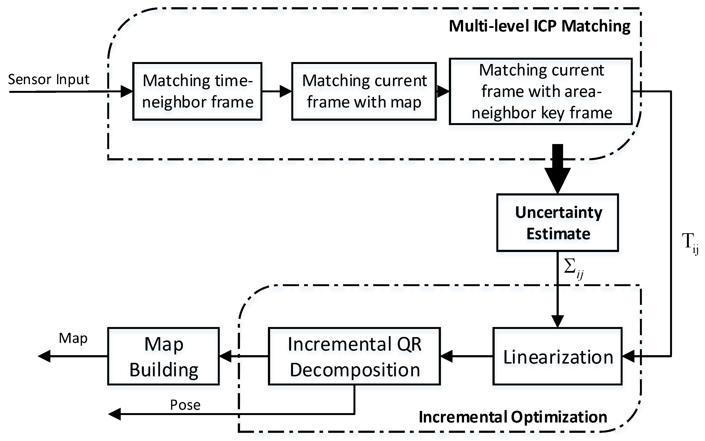
2. Algorithm Overview

Figure 1 shows the overall MIM_SLAM algorithm framework. The MIM_SLAM algorithm simplifies the SLAM problem into the data association and the incremental pose graph optimization. Firstly, the data association problem is solved by the multi-level ICP matching method which includes matching the time-neighbor frame, matching the current frame with the map, and matching the current frame with an area-neighbor keyframe. Then the uncertainty of the estimated pose is described via the Fisher information matrix. After the above steps, this algorithm can obtain the transformation matrix $T_{ij}$ and covariance matrix ${\mathsf{\Sigma }}_{ij}$ between pose $x_i$ and pose $x_j$, which can be saved in the pose graph. Finally, the incremental QR decomposition method [14] is used to optimize the pose graph. In the next section, the MIM_SLAM algorithm will be described in detail.

3. Algorithm Description

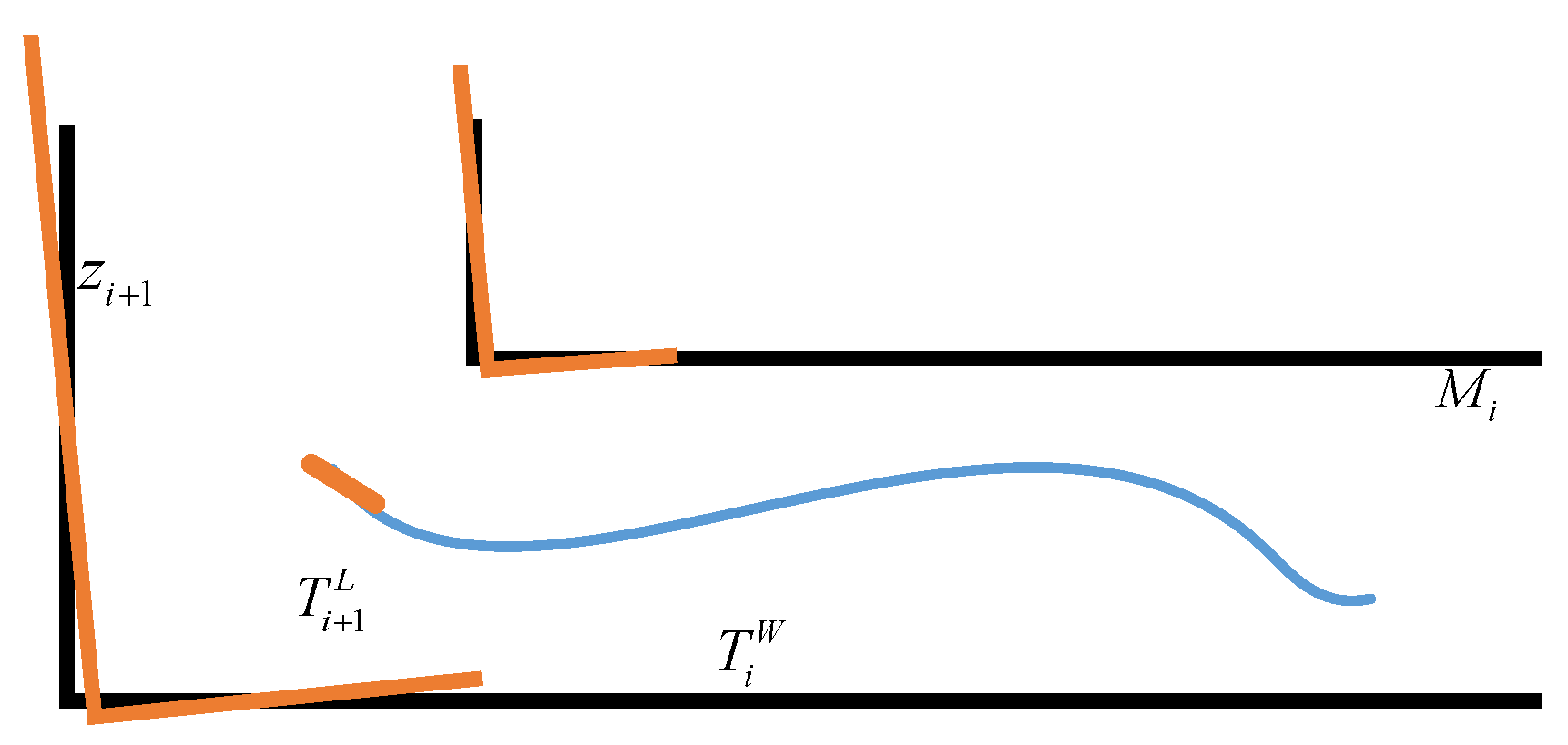
3.1. SLAM as an Incremental Optimization Problem

This part analyzes the SLAM problem from the probabilistic model and transforms the problem into a least squares problem based on the maximum a posteriori estimate. Then, the incremental QR decomposition method [17] is used to solve the least squares problem.

We denote robot pose by $X=\left\{x_i\right\}$ with $i\in 0\dots M$, the landmark by $L=\left\{l_j\right\}$ with $j\in 1\dots N$, control input given through wheeled odometry and IMU by $U=\left\{u_i\right\}$ with $i\in 1\dots M$, landmark measurement by $Z=\left\{z_i\right\}$ with $i=1\dots M$. The SLAM problem is equivalent to estimating the posterior probability distribution:

$$\begin{array}{l}P(X,L|Z,U)\\ =P(L|Z,X,U)P(X|Z,U)\\ =P(L|Z,X)P(X|Z,U)\end{array}$$

(1)

From Equation (1), it can be seen that the landmark $L$ depends on the observations and robot pose sequences, so the SLAM problem is further simplified to the pose estimation problem utilizing Baye’s rule $P(X|Z,U)=P(Z|X,U)P(X|U)/P(Z|U)$. In this paper, we just consider the online SLAM problem [4], which only involves estimating the posterior over the momentary pose, this is $P(x_M|z_{1:M},u_{1:M})$.

$$\begin{array}{l}P(x_M|z_{1:M},u_{1:M})\\ =\frac{P(z_{1:M}|x_M,u_{1:M})P(x_M|u_{1:M})}{P(z_{1:M}|u_{1:M})}\\ =\frac{P(z_M|x_M,z_{1:M-1},u_{1:M})P(x_M|z_{1:M-1},u_{1:M})}{P(z_M|z_{1:M-1},u_{1:M})}\\ =\eta P(z_M|x_M)P(x_M|z_{1:M-1},u_{1:M})\\ =\eta P(z_M|x_M){\displaystyle \int P(x_M|x_{M-1},z_{1:M-1},u_{1:M})P(x_{M-1}|z_{1:M-1},u_{1:M})d{x}_{M-1}}\\ =\eta P(z_M|x_M){\displaystyle \int P(x_M|x_{M-1},u_M)P(x_{M-1}|z_{1:M-1},u_{1:M-1})d{x}_{M-1}}\\ =\eta P(x_0){\displaystyle \prod _{i=1}^{M}P(x_i|x_{i-1},u_i)P(z_i|x_i)}\end{array}$$

(2)

In Equation (2) line 4 to 5, it is derived using the theorem of total probability. $P(x_0)$ is a prior on the initial state, $P(x_i|x_{i-1},u_i)$ is the motion model, and $P(z_i|x_i)$ is the measurement model.

To estimate the pose of the robot, we transform the SLAM problem into the least-squares problem based on the maximum a posteriori estimate. The maximum a posteriori estimate $X^{*}$ and $L^{*}$ for the trajectory and map are obtained by minimizing the negative log of the joint probability from Equation (2):

$$\begin{array}{r}{X}^{*}=\underset{X}{-\arg \min }\eta \{{\displaystyle \sum _{i=1}^M\log P(x_i|x_{i-1},u_i)}\\ +{\displaystyle \sum _{i=1}^M\log P(z_i|x_i)}\}\end{array}$$

(3)

$$L^{*}=\left\{(x_1^{*},z_1),\dots ,(x_i^{*},z_i)\right\}$$

(4)

Both of the motion model and measurement model are generally assumed such that they meet the Gaussian distribution. Then, both of them can be converted to the following form:

$$x_j\sim N(x_i\oplus T_{ij},{\mathsf{\Sigma }}_{ij})$$

(5)

where the operator $\oplus$ denotes the coordinate transformation. $T_{ij}$ and ${\mathsf{\Sigma }}_{ij}$ represent respectively the transformation matrix and covariance matrix between pose $x_i$ and pose $x_j$, which will be obtained through the multi-level ICP matching method and uncertainty estimation method in the next two paragraphs. Additionally, it can be written as follows:

$$\{\begin{array}{l}{x}_i=f(x_{i-1},u_i)+m_i\\ z_i=g(x_i)+n_i\end{array}$$

(6)

where $m_i$ is the motion noise, and $n_i$ is the measurement noise. This leads to the following nonlinear least squares problem:

$$\begin{array}{r}{X}^{*}=\underset{X}{\arg \min }\{{\displaystyle \sum _{i=1}^M{\Vert f(x_{i-1},u_i)-x_i\Vert }_{m_i}^2}\\ +{\displaystyle \sum _{i=1}^M{\Vert g(x_i)-z_i\Vert }_{n_i}^2}\}\end{array}$$

(7)

Since the above model has non-linear functions that are not easy to solve, they must be linearized, as Gauss-Newton [18] and Levenberg-Marquardt [19] has done. It can eventually be transformed into the general least-squares problem as follows, and the specific derivation can refer to the literature [14].

$${\theta }^{*}=\underset{\theta }{\arg \min }{\Vert A\theta -b\Vert }^2$$

(8)

where the vector $\theta$ contains all pose variables, and the matrix $A$ is a large and sparse Jacobian matrix.

The problem in Equation (8) is apparently solved by the Cholesky decomposition method, but the essential problem is the number of calculations involved in solving the information matrix $A^{T}A$. Thus, applying standard QR decomposition to matrix $A$:

$$A=Q\left[\begin{array}{c}R\\ 0\end{array}\right]$$

(9)

Apply Equation (9) to the least squares problem in Equation (8). As $Q$ is an orthonormal matrix, $Q^{T}Q=I$ ($I$ is identity matrix). Thus, an additional term $Q^T$ is added to the second line in (10), which doesn’t change the length of the vector $A\theta -b$.

$$\begin{array}{cc}\hfill {\Vert A\theta -b\Vert }^2& ={\Vert Q\left[\begin{array}{l}R\\ 0\end{array}\right]\theta -b\Vert }^2\hfill \\ & ={\Vert Q^{T}Q\left[\begin{array}{l}R\\ 0\end{array}\right]\theta -Q^{T}b\Vert }^2\hfill \\ & ={\Vert \left[\begin{array}{l}R\\ 0\end{array}\right]\theta -\left[\begin{array}{l}d\\ e\end{array}\right]\Vert }^2\hfill \\ & ={\Vert R\theta -d\Vert }^2+{\Vert e\Vert }^2\hfill \end{array}$$

(10)

where ${\left[d,e\right]}^T=Q^{T}b$ is defined, and (10) obtain the minimum ${\Vert e\Vert }^2$ if and only if $R\theta =d$. Now, the SLAM problem has been solved by the above analysis. However, as a new observation arrives, the Jacobian matrix $A$ does not significantly change. Thus the results of the QR decomposition at previous times can be used as the iterative initial value and the process is incremental, which can significantly reduce computational complexity.

3.2. The Multi-Level ICP Matching Method

Before detailing this method, it is useful to understand the ICP algorithm. The standard ICP [20] (Iterative Closest Point) algorithm firstly establishes the point-to-point correspondence between the two point clouds by the nearest neighbor principle and then establishes the matching error function.

Finally, it computes a transformation matrix so that the error function is minimized. In the past 30 years, many ICP variant algorithms [21] have been proposed. In this paper, an ICP variant algorithm that calls point-to-plane ICP [22] is used. Compared with the standard ICP, the robustness and accuracy are better. This algorithm is listed as Algorithm 1.

Algorithm 1: Point-to-plane ICP.

Input: Two point cloud: $A=\left\{a_i\right\}$, $B=\left\{b_i\right\}$; An initial transformation: $T_0$ Output: Transformation $T_{AB}$ which aligns $A$ and $B$; Fitness Score: $Scor{e}_{fitness}$

1: $T\leftarrow T_0$

2: while not converged do

3:   for $i\leftarrow 1toN$ do

4:     $m_i\leftarrow \mathrm{FindClosestPointInA}(T\cdot b_i)$

5:     if $\Vert m_i-T\cdot b_i\Vert \le d_{\max }$ then $w_i\leftarrow 1$

6:     else $w_i\leftarrow 0$

7:     end

8:   end

9:   $T\leftarrow \arg \min \left\{{\displaystyle \sum _i{w}_i{\Vert {\eta }_i\cdot (T\cdot b_i-m_i)\Vert }^2}\right\}$

10: end

11: $T_{AB}\leftarrow T$

12: $Scor{e}_{fitness}={{\displaystyle \sum _i{w}_i\Vert {\eta }_i\cdot (T\cdot b_i-m_i)\Vert }}^2$

The observation of the 3D LiDAR sensor is denoted as $z_k$ at time $k$. There are data associations between all previous observations $z_{1:k-1}$ and the current observation included in $z_k$. A traditional scan matching method associates $z_k$ with $z_{k-1}$ at last time, or associates $z_k$ with all previous observations $z_{1:k-1}$. These two methods either have a substantial accumulated error, or have large amounts of calculations which cannot meet online applications. In this paper, the data association is divided into two categories: continuous in time and continuous in area.

For observations that are continuous in the time, the method firstly utilizes the ICP algorithm to associate $z_k$ and $z_{k-1}$, and a rough estimation of the current robot’s pose can be obtained. The initial value of ICP is obtained by using a Kalman filter to merge the wheeled odometry with IMU. Because the inter-frame matching cannot obtain the accurate pose estimation, the next step will match the current frame with the map to further eliminate the accumulated error.

As shown in Figure 2, $M_i$ denotes the global map at time $i$ and $T_i^W$ denotes the pose of the robot in the world coordinate system at time $i$. $T_{i+1}^L$ denotes the transformation matrix from time $i+1$ to time $i$ (that is, the output of inter-frame matching). $z_{i+1}$ denotes the observation at time $i+1$. The process for matching the current frame with the map is as follows:

▪

Finding the nearest neighbor in $M_i$ for each point in $z_{i+1}$, and saving it as $m_{i+1}$. We use the combination of octree and approximate nearest neighbor algorithm in PCL [23] for speeding up.

▪

Taking $z_{i+1}$ and $m_{i+1}$ as the input of Algorithm 1, the transformation matrix $T_{opt}$ can be obtained after registering the two point clouds.

▪

The pose of the robot at time $k+1$ is $T_{i+1}^W=T_i^W\cdot T_{i+1}^L\cdot T_{opt}$.

The effectiveness of the above scan matching method is verified as shown in Figure 3. The white point clouds denote the map that SLAM has established. The blue point clouds denote the point clouds after inter-frame matching. The redpoint clouds denote the point clouds after matching the current frame with the map. It can be seen that the accumulated error in the process of inter-frame matching is obviously eliminated.

For observations that are continuous in the area, the robot returns to a region that it has previously explored. In particular, in large-scale and sparse environments, the accumulative error cannot be completely eliminated when the robot travels a long distance if only the above two matching processes are considered. So the following method matches the current frame $z_i$ with the area-neighbor keyframe $z_{\tau }$ based on a priori of pose estimation. If the matching score is less than a certain threshold, the pose constraint between $x_i$ and $x_{\tau }$ will be established. The process is listed as Algorithm 2. The initial parameter is: $L=\{(0,x_0,z_0)\}$, $d=0$.

Algorithm 2: Matching the current frame with an area-neighbor keyframe.

Input: Current pose and observation: $x_i,z_i$ Output: Transformation $T_{i\tau }$ which aligns $z_i$ and $z_{\tau }$

1: calculate $d=d+\Vert x_i-x_{i-1}\Vert$

2: if $d<d_{thre}$ then

3:    return null

4: end

5: foreach $(k_{\tau },x_{\tau },z_{\tau })$ in $L$ do

6:   if $k-k_{\tau }>k_{thre}$ then

7:     if $\Vert x_t-x_{\tau }\Vert <x_{thre}$ then

8:       put $z_t$ and $z_{\tau }$ into Algorithm 1, get $T$ and $Scor{e}_{fitness}$

9:       if $Scor{e}_{fitness}<S_{thre}$ then

10:         $T_{i\tau }\leftarrow T$

11:         return $T_{i\tau }$

12:       end

13:     end

14:   end

15: end

16: $L=L\cup (k_i,x_i,z_i),d=0,k=k+1$

17: return null

3.3. Uncertainty Estimation

After multi-level ICP matching, the transformation matrix $T_{ij}$ between pose $x_i$ and pose $x_j$ can be obtained, but we still need to know the exact uncertainty estimation, namely the covariance matrix ${\mathsf{\Sigma }}_{ij}$. However, an incorrect covariance matrix may damage the established map.

In this paper, the inversion of the Fisher information matrix is used as the covariance. The Fisher information matrix is defined as the function of the expected measurement and the surface slope scanned by the laser sensor [24]. Liu [24] and Wang [25] give the derivation of the Fisher information matrix based on a two-dimensional probability grid. It is now extended to three-dimensions. The Fisher information matrix is discretized:

$$\widehat{L}(p)={\displaystyle \sum _{i=1}^N\frac{1}{{\sigma }_i^2}{(\frac{\Delta r_{iE}}{\Delta p})}^T(\frac{\Delta r_{iE}}{\Delta p})}$$

(11)

$$\frac{\Delta r_{iE}}{\Delta p}=\left[\frac{\Delta r_{iE}}{\Delta x},\frac{\Delta r_{iE}}{\Delta y},\frac{\Delta r_{iE}}{\Delta z},\frac{\Delta r_{iE}}{\Delta \phi },\frac{\Delta r_{iE}}{\Delta \psi },\frac{\Delta r_{iE}}{\Delta \theta }\right]$$

(12)

where $p=[x,y,z,\phi ,\psi ,\theta ]$ is the pose of the robot, and ${\sigma }_{\mathrm{i}}^2$ is the noise variance of the $i$-th 3D laser range finder scan ray. $N$ is the total number of scan rays. $r_{iE}$ is the expected distance from the robot to the nearest obstacle along the $i$-th scan ray. To calculate Equation (12) efficiently, the point cloud map is converted into a three-dimensional grid map. Thus $r_{iE}$ can be computed as follows:

$$r_{iE}=\frac{{\displaystyle \sum _{j=1}^s{r}_{ij}{\mu }_{ij}}}{{\displaystyle \sum _{j=1}^s{\mu }_{ij}}}$$

(13)

where $r_{ij}$ is the distance between the robot and the $j$-th voxel along the direction of an $i$-th scan ray. ${\mu }_{ij}$ is the occupancy value of the corresponding voxel. $s$ is the sequence number of the ending voxel. By combining Equation (11) and Equation (12), we obtain:

$$\widehat{L}(p)={\displaystyle \sum _{i=1}^N\frac{1}{{\sigma }_i^2}}\left[\begin{array}{cccccc}\frac{\Delta r_{iE}^2}{\Delta x^2}& \frac{\Delta r_{iE}^2}{\Delta x\Delta y}& \frac{\Delta r_{iE}^2}{\Delta x\Delta z}& \frac{\Delta r_{iE}^2}{\Delta x\Delta \phi }& \frac{\Delta r_{iE}^2}{\Delta x\Delta \psi }& \frac{\Delta r_{iE}^2}{\Delta x\Delta \theta }\\ \frac{\Delta r_{iE}^2}{\Delta x\Delta y}& \frac{\Delta r_{iE}^2}{\Delta y^2}& \frac{\Delta r_{iE}^2}{\Delta y\Delta z}& \frac{\Delta r_{iE}^2}{\Delta y\Delta \phi }& \frac{\Delta r_{iE}^2}{\Delta y\Delta \psi }& \frac{\Delta r_{iE}^2}{\Delta y\Delta \theta }\\ \frac{\Delta r_{iE}^2}{\Delta x\Delta z}& \frac{\Delta r_{iE}^2}{\Delta y\Delta z}& \frac{\Delta r_{iE}^2}{\Delta z^2}& \frac{\Delta r_{iE}^2}{\Delta z\Delta \phi }& \frac{\Delta r_{iE}^2}{\Delta z\Delta \psi }& \frac{\Delta r_{iE}^2}{\Delta z\Delta \theta }\\ \frac{\Delta r_{iE}^2}{\Delta x\Delta \phi }& \frac{\Delta r_{iE}^2}{\Delta y\Delta \phi }& \frac{\Delta r_{iE}^2}{\Delta z\Delta \phi }& \frac{\Delta r_{iE}^2}{\Delta {\phi }^2}& \frac{\Delta r_{iE}^2}{\Delta \phi \Delta \psi }& \frac{\Delta r_{iE}^2}{\Delta \phi \Delta \theta }\\ \frac{\Delta r_{iE}^2}{\Delta x\Delta \psi }& \frac{\Delta r_{iE}^2}{\Delta y\Delta \psi }& \frac{\Delta r_{iE}^2}{\Delta z\Delta \psi }& \frac{\Delta r_{iE}^2}{\Delta \phi \Delta \psi }& \frac{\Delta r_{iE}^2}{\Delta {\psi }^2}& \frac{\Delta r_{iE}^2}{\Delta \psi \Delta \theta }\\ \frac{\Delta r_{iE}^2}{\Delta x\Delta \theta }& \frac{\Delta r_{iE}^2}{\Delta y\Delta \theta }& \frac{\Delta r_{iE}^2}{\Delta z\Delta \theta }& \frac{\Delta r_{iE}^2}{\Delta \phi \Delta \theta }& \frac{\Delta r_{iE}^2}{\Delta \psi \Delta \theta }& \frac{\Delta r_{iE}^2}{\Delta {\theta }^2}\end{array}\right]$$

(14)

According to the Cramér–Rao Bound theory [26], the lower bound of covariance can be determined by the inversion of the Fisher information matrix. Finally, the uncertainty of the pose estimation can be obtained:

$$\mathrm{cov}(p)={\widehat{L}}^{-1}(p)$$

(15)

4. Experimental Results and Analysis

As shown in Figure 4, the mobile robot called SmartGuard [27] is used to verify the proposed algorithm. It is a completely autonomous robotic system that can inspect substation equipment. SmartGuard is equipped with a wheeled odometry, an IMU, and a 3D LIDAR (RS-Lidar-16). The RS-Lidar-16 can measure out to 150 m with a high precision, $\pm$2 cm, and it has a $+$15 to $-$15-degree vertical field of view. It continuously scans the 360-degree surrounding environment at a 10 Hz frame rate and at 300,000 points/sec. The capability of the computer that runs the SLAM algorithm is as follows: Intel Core i5-6300HQ CPU 2.3 Hz and 8 G DDR3 RAM.

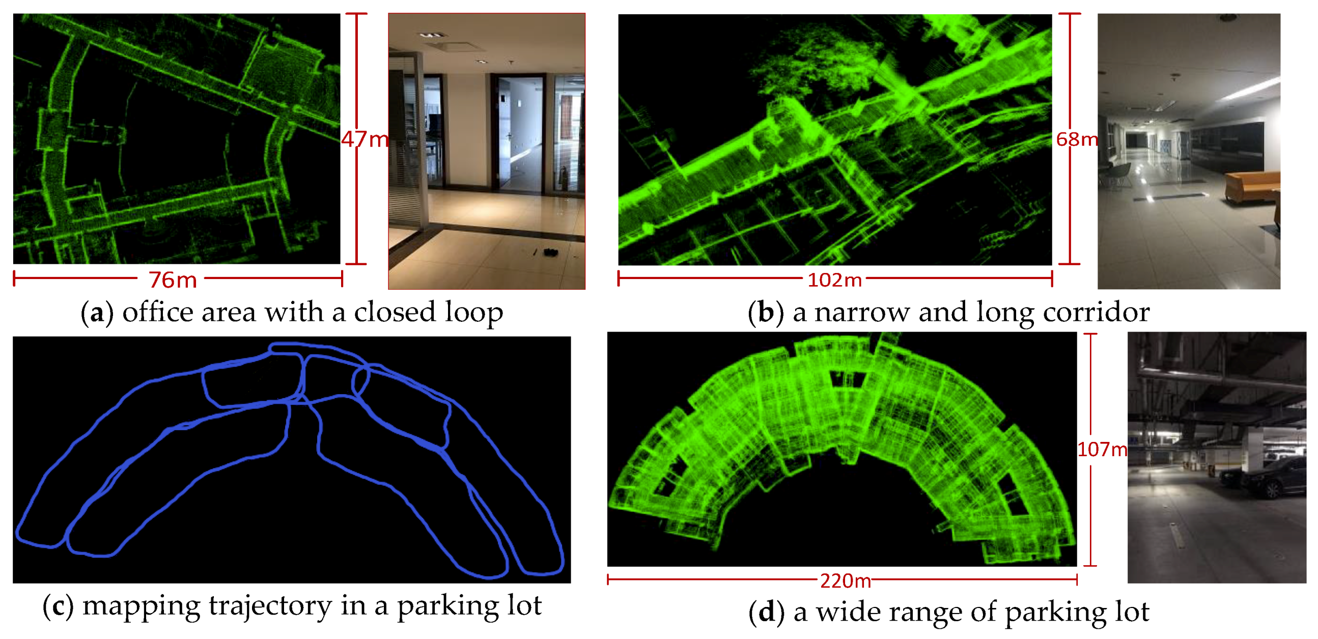
4.1. Indoor and Outdoor Mapping Test

To verify the mapping performance, the proposed algorithms have been tested in several different indoor and outdoor environments (Figure 5). Figure 5a shows that the proposed MIM_SLAM algorithm can build a consistency map with lower accumulated errors after a 180 m long loop. Figure 5b shows that the consistency map can also be generated from a narrow and long corridor. As shown in Figure 5c,d, in the wide range of the parking lot, the robot traveled approximately 1600 m at a speed of 0.6 m/s; the trajectory is shown in Figure 5c. The map shown in Figure 5c is still accurate and clear.

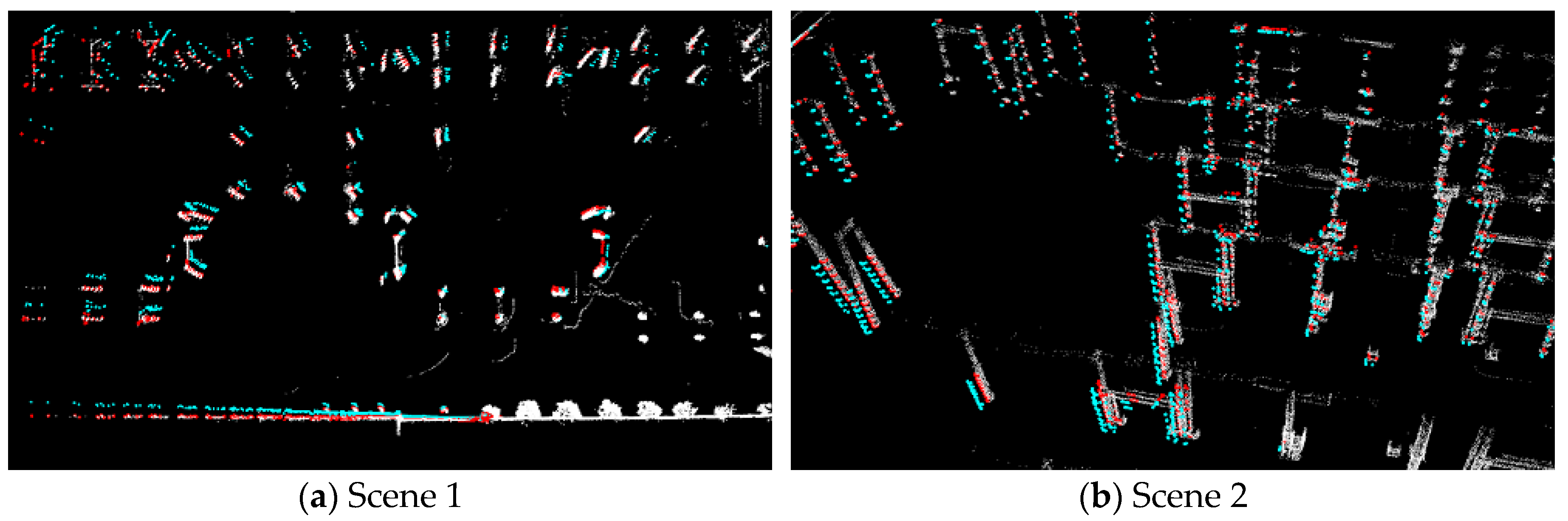
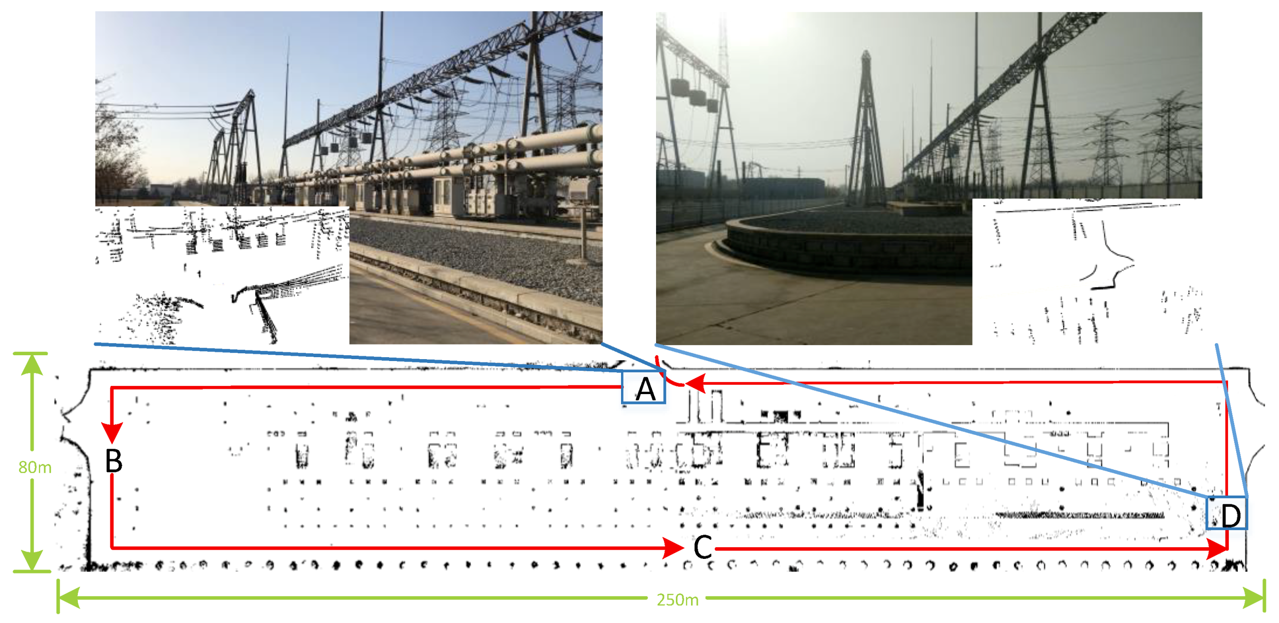
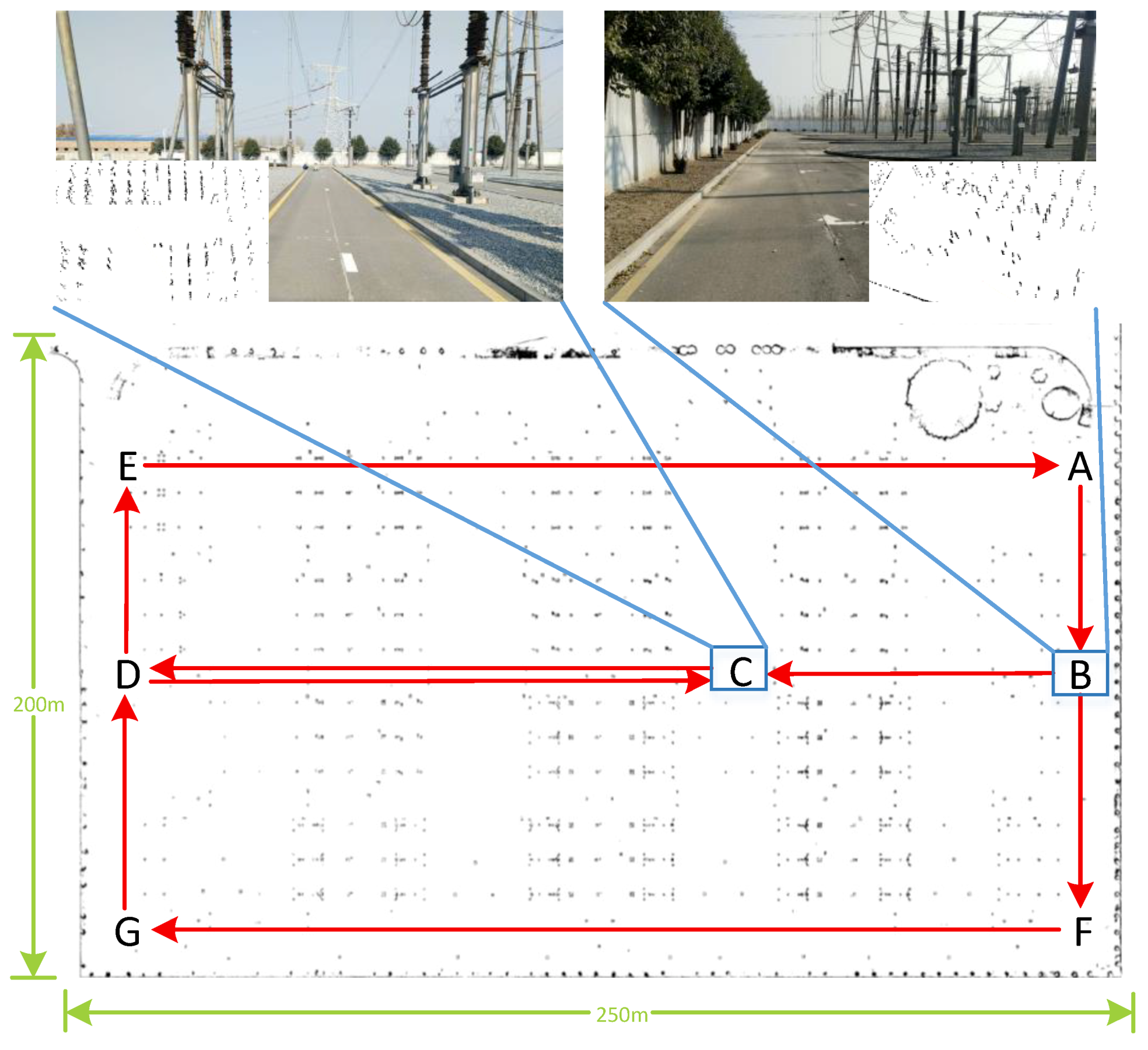
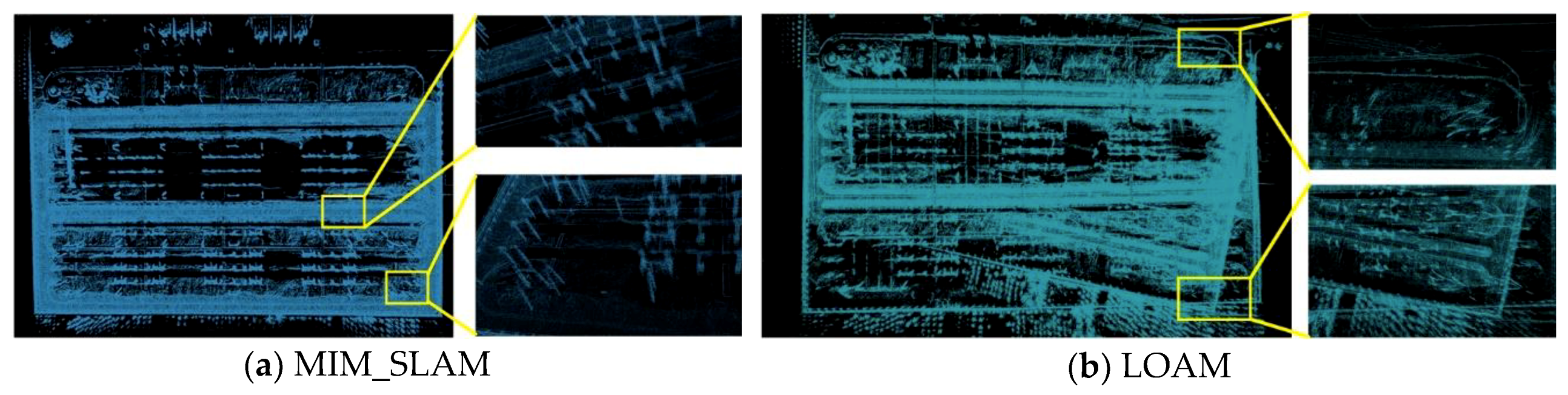
4.2. Large-Scale and Sparse Scenes Test

Two substations are selected to verify the validity of the MIM_SLAM algorithm in the larger-scale and sparse environments. A general substation comprises thousands of square meters, and its electrical equipment needs to include a sufficient distance for electrical safety. We first tested in substation A shown in Figure 6. During the experiment, the robot traveled approximately 600 m at a speed of 0.6 m/s and the 3D LIDAR sensor collected a total of 10,080 frames. The plan and the environment of substation A are shown in Figure 6. The red line denotes the robot’s trajectory ABCDA. The point cloud maps established by the MIM_SALM and the LOAM [12] which has been considered state-of-the-art in LiDAR SLAM are shown in Figure 7.

Intuitively, the MIM_SLAM algorithm has a high consistency map compared with the LOAM. Due to the accumulated error, the estimated pose has a great deviation when the robot travels from area A along the red track shown in Figure 6, and then returns back to area A. The LOAM cannot effectively handle the data association at this moment, which leads to the wrong association and damage to the established map. In this paper, the multi-level ICP matching method takes into account this situation and generates a reliable constraint between the two poses. The incremental optimization method is used to optimize the global pose. Thus the final map has a high consistency.

Next, we tested it in substation B. Compared with substation A, this was larger. Meanwhile, the electrical equipment is placed more sparsely, and less information is gathered by the 3D LIDAR sensor. During the experiments, the robot traveled approximately 1450 m at a speed of 0.6 m/s, and the LIDAR sensor collected a total of 24,220 frames. The plan and the environment of substation B are shown in Figure 8. The red line denotes the robot’s trajectory ABCDEABFGDC. The point cloud maps established by the MIM_SLAM algorithm and the LOAM are shown in Figure 9.

It can be seen from the observation of the two scenes given in Figure 8 that the electrical equipment is distributed more sparsely, and more than 70% of the laser rays reach the maximum measurement range. As shown in Figure 9a, both contour lines of the map established by the MIM_SLAM algorithm are at right angles at areas F and G. Additionally, when the robot returned back to the area C, the details of the point cloud map at area C showed that the telegraph poles and the road edge are clearly visible, and there is no incorrect point cloud accumulation. Because the LOAM cannot effectively process the data association of the closed-loop area, the performance is very poor in this situation, which has more closed-loop areas in large-scale environments, as shown in Figure 9b.

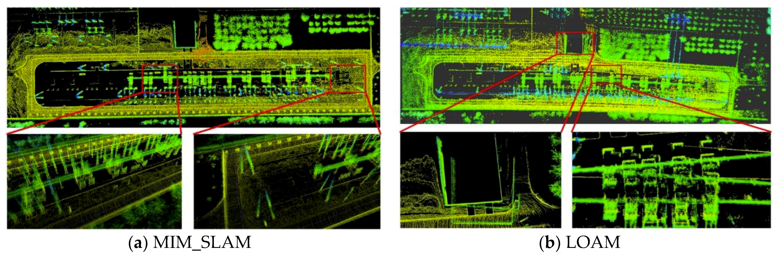
4.3. Mapping Accuracy Test

In order to analyze the mapping accuracy quantitatively, we selected two substations with large-scale and sparse characteristics which are shown in Figure 6 and Figure 8, also the standard ICP [20] and the LOAM [12] algorithm was selected to compare with the MIM_SLAM algorithm. In the experiments, the robot is controlled running at a speed of 0.6 m/s on a flat road along a straight line with a length of 10 m. The accuracy of mapping is defined as the robot’s localization error $\epsilon$ [28], expressed as follows:

$$\begin{array}{c}\epsilon =\frac{1}{N}{\displaystyle \sum _{i=0}^{N-1}\Vert e_i\Vert }\\ e_i=(x_0\oplus T_i)-(x_0^{\ast }\oplus T_i^{\ast })\end{array}$$

(16)

where $x_0$ and $x_0^{\ast }$ denote the initial pose. $\oplus$ is the standard motion composition operator. $T_i$ denotes the transformation matrix of the estimated pose $x_i$ relative to the initial pose $x_0$. $T_i^{\ast }$ denotes the transformation matrix of the true pose $x_i^{\ast }$ relative to the initial pose $x_0^{\ast }$. $\Vert ·\Vert$ is the 2-Norm used in this paper. For the robot to navigate in three-dimensional environments, $e_i$ is represented as $(x_e,y_e,z_e,{\phi }_e,{\psi }_e,{\theta }_e)$. Then $\epsilon$ can be divided into two parts: translation error and rotation error.

$$\epsilon =\frac{1}{N}{\displaystyle \sum _{i=0}^{N-1}\Vert trans(e_i)\Vert }+\frac{1}{N}{\displaystyle \sum _{i=0}^{N-1}\Vert rot(e_i)\Vert }$$

(17)

Since it is difficult to obtain the true pose of the robot, 20 points are selected from the robot’s trajectory. The first point is taken as the initial pose. For the next 19 points, the difference value of the localization results relative to the initial pose is calculated. The difference value of the true pose can be measured by the tape. In

Table 1. The localization error results of different approaches/scenes.

	Standard ICP	LOAM	MIM_SALM
	Trans. Error (unit: m)
A	0.213 ± 0.148	0.064 ± 0.057	0.052 ± 0.043
B	0.282 ± 0.177	0.075 ± 0.066	0.066 ± 0.062
	Rot. Error (unit: deg)
A	2.5 ± 1.9	1.8 ± 1.2	1.6 ± 1.4
B	3.1 ± 2.2	2.5 ± 2.1	2.2 ± 1.8

, the localization error is tested with the standard ICP, the LOAM and the MIM_SLAM algorithms under substation A and B. It can be seen that the MIM_SLAM algorithm is more precise. If there is a closed-loop area on the robot’s path, the MIM_SLAM algorithm will be better than the LOAM. The processing time per frame using different approaches is calculated and shown in

Table 2. The average time consumption per frame for different approaches/scenes.

	Standard ICP	LOAM	MIM_SALM
	Processing Time (unit: s)
A	0.0405	0.1036	0.0886
B	0.0416	0.1067	0.0932

. MIM_SLAM has a similar time consuming compared to the LOAM and meets the real-time requirements. In Section 4.4, this will be further analyzed in the benchmark dataset.

4.4. Benchmarking Datasets Test

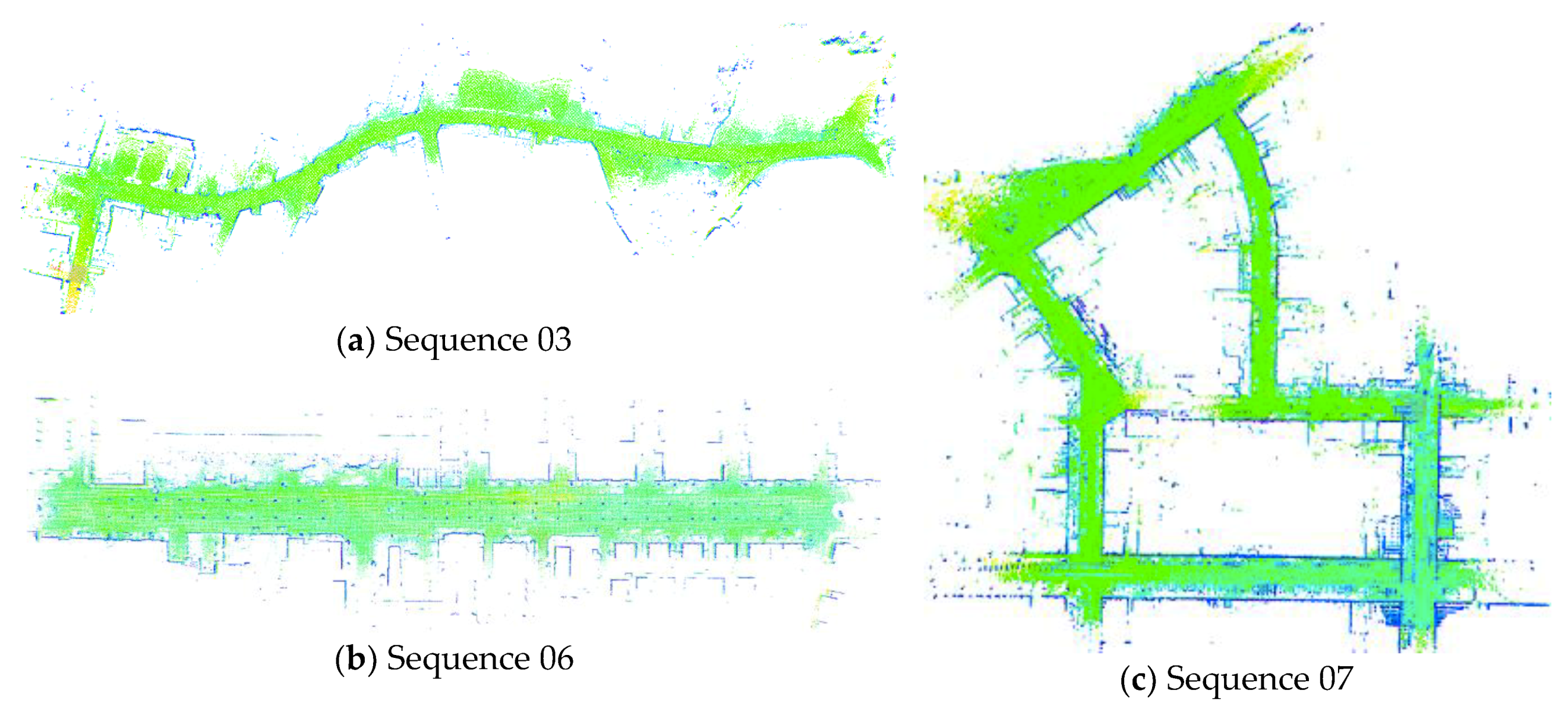
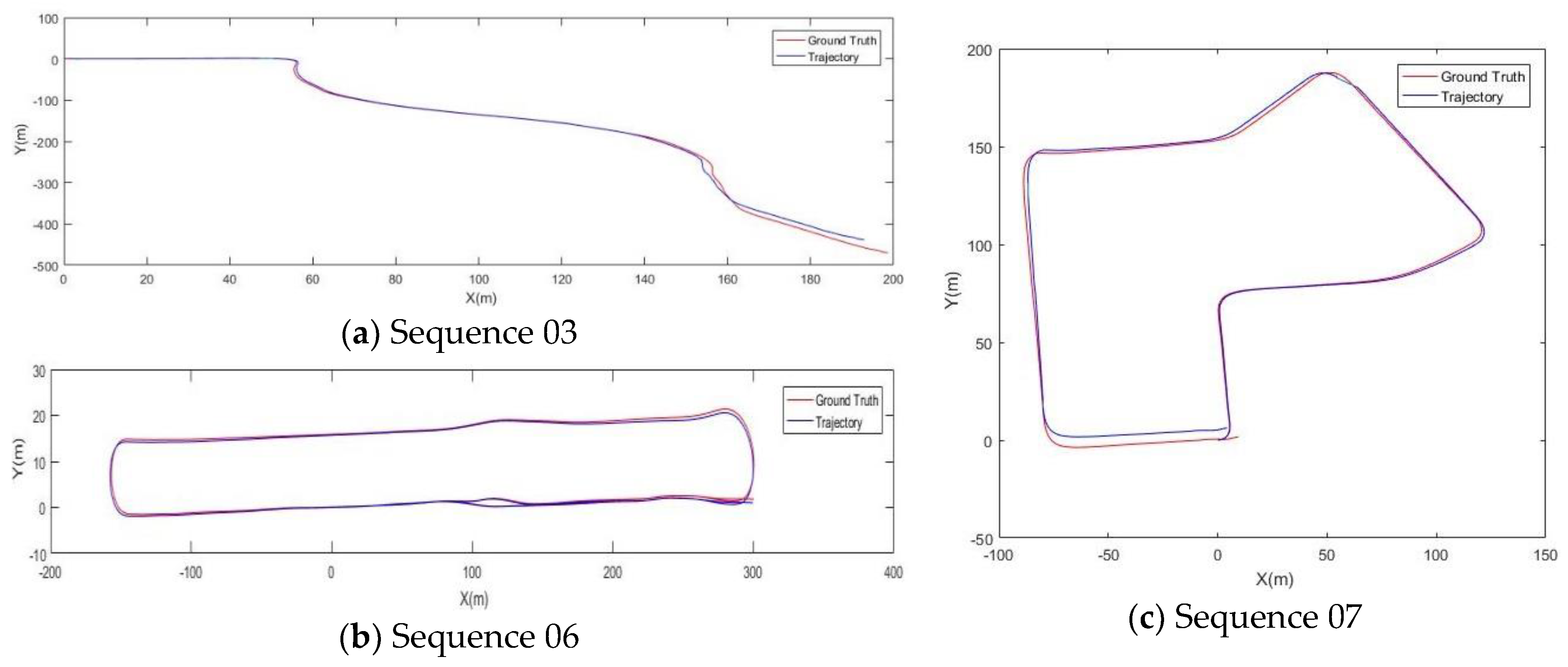
Then, datasets from the KITTI odometry benchmark [29] are used to evaluated MIM_SLAM. The datasets take advantage of the autonomous driving platform Annieway to develop novel challenging real-world computer vision benchmarks. The autonomous driving platform is equipped with a 360° Velodyne HDL-64E laser scanner and two high-resolution color and grayscale video cameras. Accurate ground truth is provided by a GPS localization system. We selected three typical types of environments: “urban” with building around (sequence 07), “country” on small roads with vegetation in this scene (sequence 03), and “highway” where roads are wide and lower dynamic (sequence 06).

(1)

Sequence 03: This dataset is designed to verify that MIM_SLAM can achieve a low drift pose estimation in sparse vegetation environment. The mapping result is shown in Figure 10a and the trajectory and the ground truth are shown in Figure 11a. Due to the scarce stable features in this scene, there is a bit of position deviation after 420 m of traveling compared with the ground truth in Figure 11a. To evaluate the pose estimation accuracy, we use the evaluation method in the KITTI odometry benchmark which calculated the translational and rotational errors for all possible subsequences of length (100, 200, …, 800) meters. As is shown in Figure 12a, both LOAM and MIM_SLAM achieve lower drift values compared with the standard ICP method, and MIM_SLAM is slightly worse than LOAM.

(2)

Sequence 06: We use this dataset to verify that MIM_SLAM can effectively process the data association of the closed-loop area shown in Figure 10b and Figure 11b. From Figure 12b, it can be seen that the translational and rotational errors are lower compared to the standard ICP, and slightly better than LOAM.

(3)

Sequence 07: This urban road scene is highly dynamic and large-scale. The vehicle travels approximately 660 m at a speed of 6.2 m/s. The mapping result is shown in Figure 10c and the trajectory and the ground truth are shown in Figure 11c. Intuitively, the details of the point cloud map are clear. The estimated pose and the ground truth are almost overlapping. The pose estimation error is shown in Figure 12c quantitatively.

5. Conclusions

For large-scale and sparse environments, we propose a novel MIM_SLAM algorithm in this paper, which simplifies the SLAM problem to the least-squares optimization problem. The contribution of this paper is that the multi-level ICP matching method is proposed to solve the data association problem and the uncertainty estimation is handled by the Fisher information matrix. It considers the accumulated errors in two aspects: matching between time-neighbor frames (building a low-drift LiDAR odometry) and matching between area-neighbor frames (dealing with the data association at a revisited area). Moreover, multi-level matching and incremental optimization reduce the computational complexity while ensuring mapping accuracy, we can achieve accurate mapping and real-time applications. Additionally, its application is not only limited to mobile robots, and it can potentially be extended to other vehicles, e.g., UAVs. Experimental results show that it can effectively build a high consistency map with a smaller amount of environmental information and the large-scale scenes, and it also achieves similar or better accuracy compared with the standard ICP and the state-of-the-art LOAM algorithm in the KITTI dataset. Additionally, there are some limitations in high dynamic scenes. Our future work will focus on the construction of a more robust data association method, we will integrate the output of our multi-level ICP matching with an IMU in a Kalman filter to further reduce the accumulated error.

References

1. Martínez, J.L.; Morán, M.; Morales, J.; Reina, A.J.; Zafra, M. Field Navigation Using Fuzzy Elevation Maps Built with Local 3D Laser Scans. Appl. Sci. 2018, 8, 397. [Google Scholar] [CrossRef]
2. Smith, R.; Cheeseman, P. On the Estimation and Representations of Spatial Uncertainty. Int. J. Robot. Res. 1987, 5, 56–68. [Google Scholar] [CrossRef]
3. Shinsuke, M.M.D.; Noboru, I.M.D.; Yoshito, I.M.D. Estimating Uncertain Spatial Relationships in Robotics. Mach. Intell. Pattern Recognit. 2013, 5, 435–461. [Google Scholar]
4. Thrun, S.; Liu, Y.; Koller, D.; Ng, A.Y.; Ghahramani, Z.; Durrant-Whyte, H. Simultaneous localization and mapping with sparse extended information filters. Int. J. Robot. Res. 2004, 23, 693–716. [Google Scholar] [CrossRef]
5. Montemerlo, M.S. Fastslam: A factored solution to the simultaneous localization and mapping problem with unknown data association. Arch. Environ. Contam. Toxicol. 2015, 50, 240–248. [Google Scholar]
6. Gutmann, J.S.; Konolige, K. Incremental mapping of large cyclic environments. In Proceedings of the 1999 IEEE International Symposium on Computational Intelligence in Robotics and Automation (CIRA ’99), Monterey, CA, USA, 8–9 November 2002; pp. 318–325. [Google Scholar] [Green Version]
7. Zlot, R.; Bosse, M. Efficient large-scale 3D mobile mapping and surface reconstruction of an underground mine. In Field and Service Robotics; Springer: Berlin/Heidelberg, Germany, 2014; pp. 479–493. [Google Scholar]
8. Olufs, S.; Vincze, M. An efficient area-based observation model for monte-carlo robot localization. In Proceedings of the 2009 IEEE/RSJ International Conference on Intelligent Robots and Systems (IROS 2009), St. Louis, MO, USA, 10–15 October 2009; pp. 13–20. [Google Scholar]
9. Huang, S.; Wang, Z.; Dissanayake, G. Sparse local submap joining filter for building large-scale maps. IEEE Trans. Robot. 2008, 24, 1121–1130. [Google Scholar] [CrossRef] [Green Version]
10. Moosmann, F.; Stiller, C. Velodyne slam. In Proceedings of the 2011 IEEE Intelligent Vehicles Symposium (IV), Baden, Germany, 5–9 June 2011; pp. 393–398. [Google Scholar]
11. Nüchter, A.; Lingemann, K.; Hertzberg, J.; Surmann, H. 6D SLAM-3D mapping outdoor environments. J. Field Robot. 2007, 24, 699–722. [Google Scholar] [CrossRef]
12. Zhang, J.; Singh, S. LOAM: Lidar Odometry and Mapping in Real-time. In Proceedings of the 2014 Robotics: Science and Systems, Berkeley, CA, USA, 12–16 July2014; Volume 2. [Google Scholar]
13. Wang, J.; Li, L.; Zhe, L.; Weidong, C. Multilayer matching SLAM for large-scale and spacious environments. Int. J. Adv. Robot. Syst. 2015, 12, 124. [Google Scholar] [CrossRef]
14. Liu, Z.; Chen, H.; Di, H.; Tao, Y.; Gong, J.; Xiong, G.; Qi, J. Real-Time 6D Lidar SLAM in Large Scale Natural Terrains for UGV. In Proceedings of the 2018 IEEE Intelligent Vehicles Symposium (IV), Changshu, China, 26–30 June 2018; pp. 662–667. [Google Scholar]
15. Liang, X.; Chen, H.; Li, Y.; Liu, Y. Visual laser-SLAM in large-scale indoor environments. In Proceedings of the IEEE International Conference on Robotics and Biomimetics, Qingdao, China, 3–7 December 2017; pp. 19–24. [Google Scholar]
16. Hess, W.; Kohler, D.; Rapp, H.; Andor, D. Real-time loop closure in 2D LIDAR SLAM. In Proceedings of the IEEE International Conference on Robotics and Automation, Stockholm, Sweden, 16–21 May 2016; pp. 1271–1278. [Google Scholar]
17. Kaess, M.; Ranganathan, A.; Dellaert, F. iSAM: Incremental smoothing and mapping. IEEE Trans. Robot. 2008, 24, 1365–1378. [Google Scholar] [CrossRef]
18. Hartley, H.O. The modified Gauss-Newton method for the fitting of non-linear regression functions by least squares. Technometrics 1961, 3, 269–280. [Google Scholar] [CrossRef]
19. Moré, J.J. The Levenberg-Marquardt algorithm: Implementation and theory. In Numerical Analysis; Springer: Berlin/Heidelberg, Germany, 1978; pp. 105–116. [Google Scholar]
20. Besl, P.J.; Mckay, N.D. Method for registration of 3-D shapes. IEEE Trans. Pattern Anal. Mach. Intell. 2002, 14, 239–256. [Google Scholar] [CrossRef]
21. Li, L.; Liu, J.; Zuo, X.; Zhu, H. An Improved MbICP Algorithm for Mobile Robot Pose Estimation. Appl. Sci. 2018, 8, 272. [Google Scholar] [CrossRef]
22. Chen, Y.; Medioni, G. Object modelling by registration of multiple range images. Image Vis. Comput. 1992, 10, 145–155. [Google Scholar] [CrossRef]
23. Rusu, R.B.; Cousins, S. 3D is here: Point Cloud Library (PCL). In Proceedings of the 2011 IEEE International Conference on Robotics and Automation, Shanghai, China, 9–13 May 2011; pp. 1–4. [Google Scholar]
24. Liu, Z.; Chen, W.; Wang, Y.; Wang, J. Localizability estimation for mobile robots based on probabilistic grid map and its applications to localization. In Proceedings of the 2012 IEEE Conference on Multisensor Fusion and Integration for Intelligent Systems (MFI), Hamburg, Germany, 13–15 September 2015; pp. 46–51. [Google Scholar]
25. Wang, Y.; Chen, W.; Wang, J.; Wang, H. Active global localization based on localizability for mobile robots. Robotica 2015, 33, 1609–1627. [Google Scholar] [CrossRef]
26. Bobrovsky, B.; Zakai, M. A lower bound on the estimation error for certain diffusion processes. IEEE Trans. Inf. Theory 1976, 22, 45–52. [Google Scholar] [CrossRef]
27. Wang, B.; Guo, R.; Li, B.; Han, L.; Sun, Y.; Wang, M. SmartGuard: An autonomous robotic system for inspecting substation equipment. J. Field Robot. 2012, 29, 123–137. [Google Scholar] [CrossRef]
28. Burgard, W.; Stachniss, C.; Grisetti, G.; Steder, B.; Kümmerle, R.; Dornhege, C.; Ruhnke, M.; Kleiner, A.; Tardös, J.D. A comparison of SLAM algorithms based on a graph of relations. In Proceedings of the 2009 IEEE/RSJ International Conference on Intelligent Robots and Systems (IROS 2009), St. Louis, MO, USA, 10–15 October 2009; pp. 2089–2095. [Google Scholar]
29. Geiger, A. Are we ready for autonomous driving? The KITTI vision benchmark suite. In Proceedings of the 2012 Computer Vision and Pattern Recognition, Providence, RI, USA, 16–21 June 2012; pp. 3354–3361. [Google Scholar]
Figure 1. The proposed MIM_SLAM algorithm framework.
Applsci 08 02432 g001
Figure 2. The matching process of the current frame and map.
Applsci 08 02432 g002
Figure 3. An example of the matching process.
Applsci 08 02432 g003
Figure 4. The mobile robot (SmartGuard) for experiments.
Applsci 08 02432 g004
Figure 5. The maps generated in the indoor and outdoor environments.
Applsci 08 02432 g005
Figure 6. The plan and the environment of substation A.
Applsci 08 02432 g006
Figure 7. The point cloud maps established by the MIM_SLAM and the LOAM [12] algorithms.
Applsci 08 02432 g007
Figure 8. The plan and the environment of substation B.
Applsci 08 02432 g008
Figure 9. The point cloud maps established by the MIM_SLAM and the LOAM algorithms.
Applsci 08 02432 g009
Figure 10. The mapping results in the three sequences.
Applsci 08 02432 g010
Figure 11. The trajectory produced by MIM_SLAM in the three sequences.
Applsci 08 02432 g011
Figure 12. The pose estimation error in the three sequences.
Applsci 08 02432 g012