Numerical Study on Evaluating the Concrete-Bedrock Interface Condition for Hydraulic Tunnel Linings Using the SASW Method

Abstract

The current methods for evaluating the contact condition between concrete and lining were the ground penetrating radar (GPR) and the coring method. The penetration of radar electromagnetic waves was greatly affected by steel reinforcement and water, which often made the detection results of GPR unsatisfactory. A spectral analysis of the surface wave (SASW) method was used to evaluate the concrete-bedrock interface condition for hydraulic tunnel linings in this paper, since the impact elastic wave is less affected by steel bars and water content. An SASW implementation program based on fast Fourier transformation (FFT) was developed to analyze data from numerical simulations and field tests. Various models were studied to investigate the feasibility of using numerical analysis. For the first time, the study was employed to find out the influences of different receiver spacings and impact duration on the efficiency of detecting the existence of a weak layer underneath the concrete using the SASW method. On this basis, in-situ tests were carried out to verify the applicability in the field and results were verified by coring. In the research, the following results were found: (1) The finite element analysis results of different uniform or layered models showed that the SASW method could accurately identify the interface contact condition between the concrete lining and bedrock, especially the existence of voids; (2) when the receiver spacing was 1.0–1.5 times the thickness of the target object to be inspected, the quality of the collected signal data was the best; (3) under a certain reasonable range, the impact duration had an insignificant effect on the phase spectra and dispersion curves of a concrete-weak layer model; (4) in-situ SASW inspection could accurately tell whether the voids exist at the concrete-bedrock interface; and (5) the data processing program of the SASW method based on the MATLAB platform was accurate, convenient, and worth promoting.

1. Introduction

The shortage of water resources has constrained the sustainable development of China’s economy and the long-term stability of society in recent years. Inter-basin water transfer is one of the effective measures that can be employed to alleviate the regional water shortage in China. The hydraulic tunnel is an important part of the water delivery building. To ensure the safe and efficient operation, a concrete lining is usually imperative. However, factors such as over-excavation, under-excavation, and poor site management during tunnel construction may cause potential defects, such as a lack of thickness, voids at the lining-bedrock interface, and incompact concrete of the tunnel lining. In order to reduce or even eliminate these defects, and make sure that the tunnels are safe after operation, ground penetrating radar (GPR), as an effective detection technique, has been widely applied to tunnel inspection, and has achieved good results [1]. Some voids at the lining-bedrock interface can be found, but the penetration of radar electromagnetic waves is greatly affected by steel reinforcement and water due to the skin effect, which often results in unsatisfactory detection [2,3]. Moreover, a destructive inspection method like coring will cause unnecessary damage to the lining, which may induce some additional artificial defects to the concrete. Therefore, a new non-destructive inspection method is needed to cover the shortage of GPR.

The impact elastic wave is less affected by steel bars and water content because it has the characteristics of a large vibration energy, simple operation, and is convenient for spectrum analysis, etc. Therefore, it is very suitable for the non-destructive inspection of structures. An impact elastic wave is excited by physical means, such as hammer impact or electromagnetic excitation [4]. Since the object being tested is slightly deformed and still in an elastic state, the vibration can be regarded as a result of the elastic wave propagation. The schematic elastic wave propagation generated by impact excitation (Figure 1) mainly includes compression wave P, shear wave S, and Rayleigh wave R [5]. The R-wave is a surface wave propagating along the free surface of the elastic medium. Compared with the P-wave and the S-wave, the R-wave has the largest energy and the smallest attenuation [6,7,8]. Therefore, the R-wave (surface wave) signal is easier to collect when carrying out testing on pavement systems [9,10] and concrete surfaces [11]. Generally, the excitation source is divided into two categories: steady-state forced vibration and transient impact. As a result, the corresponding surface wave analysis is also divided into two types: the steady-state method and transient method. In this paper, only the transient surface wave method is studied since, in the field, it is very hard to implement steady-state excitation on the tunnel lining, especially on the crowned arch.

At present, there are two main analytical methods commonly used for transient surface waves: the spectral analysis of the surface wave (SASW) method; and the multichannel transient R-wave methods, like the multichannel analysis of surface waves (MASW) and frequency-wavenumber (F-K) [13,14]. The SASW method was originally proposed by Nazarian and Stoke in 1985 for a seismic wave test analysis method for detecting the shear wave propagation properties of soil layers and pavements, and later it was adopted in the inspection and safety evaluation of concrete structures [15,16,17,18,19]. The SASW method includes surface wave generation and processing of transducer received data. The typical test arrangement of the SASW method is shown in Figure 2. An impact is applied to the surface of the medium to be tested by the impact hammer to generate elastic waves with a certain frequency range [20]. The R-waves of different frequencies are superimposed on each other and spread together on the surface of the medium at the same time. By performing spectrum analysis on the R-wave time domain signals received by the two transducers, the R-waves of the respective frequencies f are separated, and the R-wave velocity V_R of each frequency f is calculated, thereby the dispersion curve V_R~λ_R is obtained [21,22,23]. SASW is rarely used to evaluate the concrete-bedrock interface condition for hydraulic tunnel linings. Moreover, when the post-processing software of the equipment is used to analyze the phase unwrapping, the unreasonable data cannot be eliminated, and the obvious misjudgment usually results in unsatisfactory test results.

In this paper, a numerical study on evaluating the concrete-bedrock interface condition for hydraulic tunnel linings using the SASW method is introduced. An SASW implementation program based on FFT is developed, and all data analyses in this study are done using this program. For signals collected by the sensor, it can be automatically interpreted by the program to obtain the dispersion curve and the interference can also be artificially eliminated to make the result more reasonable. The finite element simulation is carried out to verify the feasibility of SASW to evaluate the concrete-bedrock interface condition. For the first time, the study is able to find out the influences of different receiver spacings and impact duration on the efficiency of detecting the existence of a weak layer underneath the concrete. On this basis, the effects of different contact times and different track spacing values on the detection accuracy are studied. The accuracy of this method is verified by a field test.

2. Materials and Methods

2.1. Processing Method of Collecting Signals

In Figure 2, the R-wave signals V₁(t) and V₂(t) picked up by the two receivers (normally accelerators) are excited by the same impact source, so V₂(t) can be regarded as the repeat of V₁(t) after a time delay of ∆t (∆t = d/V_R). Therefore, the V₂(t) signal can be added with a time delay τ to calculate the cross-correlation function r₁₂(τ) of the two signals to evaluate their coherence [24,25,26].

$$r_{21}\left(\tau \right)=\underset{-\infty }{\overset{+\infty }{{\displaystyle \int }}}{V}_2\left(t+\tau \right)V_1\left(t\right)dt$$

(1)

Then, the Fourier transform is used to calculate the cross-power spectrum of the two signals, from which the phase-difference spectrum (hereinafter simply put as phase spectrum) can be obtained (see Equation (2)). This phase spectrum is used to read the phase difference at different frequencies, and the R-wave dispersion curve is then formed.

$$\begin{array}{ll}\hfill F_{21}(\omega )& = {\displaystyle {\int }_{-\infty }^{+\infty }{r}_{21}(\tau )e^{-i\omega \tau }d\tau }={\displaystyle {\int }_{-\infty }^{+\infty }({\displaystyle {\int }_{-\infty }^{+\infty }{v}_2(t+\tau )v_1(t)dt}})e^{-i\omega \tau }d\tau \hfill \\ & = {\displaystyle {\int }_{-\infty }^{+\infty }{v}_2(t+\tau )e^{-i\omega (t+\tau )}d(t+\tau )}{\displaystyle {\int }_{-\infty }^{+\infty }{v}_1(t)e^{i\omega t}dt}=F_2(\omega )F_1^{*}(\omega )\hfill \\ & = \left|F_2(\omega )\right|e^{i{\varphi }_2}\left|F_1(\omega )\right|e^{-i{\varphi }_1}=\left|F_2(\omega )\right|\left|F_1(\omega )\right|e^{i({\varphi }_2-{\varphi }_1)}=\left|F_{21}(\omega )\right|e^{i\Delta \varphi (\omega )}\hfill \end{array}$$

(2)

where F₂₁(ω) represents the Fourier transform for the cross-correlation function r₁₂(τ), which is the cross-power spectrum of the two signals V₁(t) and V₂(t); F₁(ω) and F₂(ω) represent the Fourier transforms of the two signals V₁(t) and V₂(t), respectively; and F₁*(ω) represents the complex conjugate of F₁(ω).

The propagation time difference of the signals between two receivers is:

$$\Delta t=\left(\Delta \varphi /2\pi \right)T=\Delta \varphi /\left(2\pi f\right)$$

(3)

The R-wave velocities at different frequencies are:

$$v_R=2\pi fd/\Delta \varphi$$

(4)

The relationship between R-wave velocity, wavelength, and frequency is:

$$v_R={\lambda }_{R}f$$

(5)

Combining Equations (3) and (4), the R-wave length can be calculated as follows:

$${\lambda }_R=2\pi d/\Delta \varphi$$

(6)

where, for Equations (3) and (6), V_R is the R-wave velocity, λ_R is the R-wave length, f represents the frequencies along the phase cycles on the phase spectrum, ∆φ is the unwrapped phase difference (in radians) corresponding to f, and d is the receiver spacing.

An SASW implementation program based on FFT was developed with Matlab (MATLAB Release 2018b, The MathWorks, Inc., Natick, MA., USA) [27,28,29,30,31]. The analysis procedure flow-chart is shown in Figure 3. All data analyses in this study were conducted using this program.

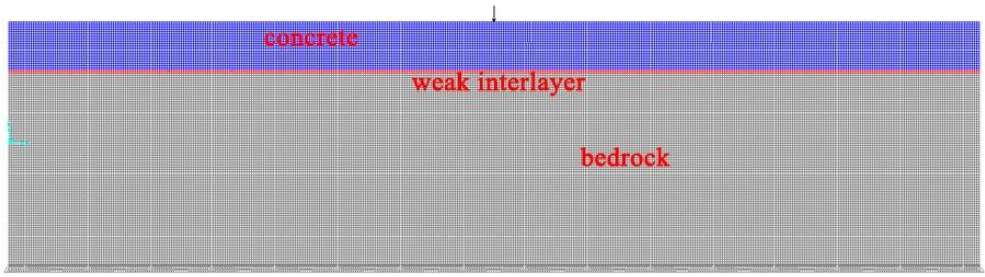
2.2. Description of Finite Element Calculation

Finite element analysis was performed to investigate the feasibility of using the SASW method to evaluate the lining-bedrock interface condition. The plane model had a dimension of 8 m wide and 2 m deep, and a uniform element size of 2 cm was adopted, as shown in Figure 4. Four different model schemes were created, as shown in

Table 1. Model schemes.

Number	Material	Thickness (cm)	Model Type
1	concrete	200	Uniform
2	concrete	40	Layered model 1
	bedrock	160
3	concrete	40	Layered model 2
	weak interlayer	2
	bedrock	158
4	concrete	40	Layered model 3
	weak layer	160

. The material properties are listed in

Table 2. Material properties.

Material	Dynamic Elastic Modulus (GPa)	Poisson’s Ratio	Density (kg/m3)
concrete	30	0.2	2450
bedrock	10	0.3	2500
weak interlayer	1	0.3	-
weak layer	1	0.3	-

. The weak interlayer was used to simulate a real case scenario when there was very poor bonding between the lining and the surrounding rock, which often happened at the two sidewalls and the bottom of the lining due to insufficient treatment of the excavated rock surface. The weak layer intended to simulate the case where there was a total separation (void) outside the lining, which typically happened at the top arch of the lining due to over-excavation of the bedrock. The layered concrete-weak interlayer-bedrock model is shown in Figure 5. The hammer impact was simulated by applying a 0.5 KN-magnitude impulse point-load with a half-cycle sine curve of force-time history at the top middle node of the model, in which the time span of the impulse represented the impact duration.

Linear transient modal time history analysis was conducted. Vertical accelerations were picked up at two receivers shown in Figure 4. The sampling interval at the receiver locations was 5 us and the total number of sampling points was 1024. Cross-power spectrum analysis of the signals of these two channels was then performed using Matlab to generate phase spectra and the corresponding R-wave velocity dispersion curves.

The theoretical R-wave velocity of concrete can be obtained from Equation (7), which is calculated to be 2059 m/s using the parameters in Table 2.

$$V_R=\frac{0.87+1.12\mu }{1+\mu }\sqrt{\frac{E_d}{2\rho \left(1+\mu \right)}}$$

(7)

where E_d is the dynamic elastic modulus, ρ is the density, and μ is the Poisson’s ratio of concrete.

3. Results and Discussion

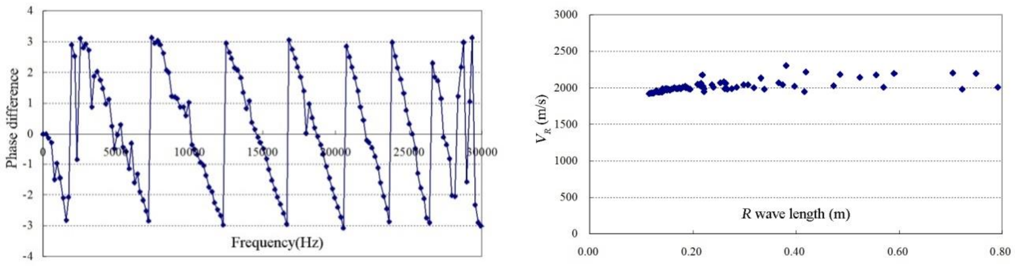
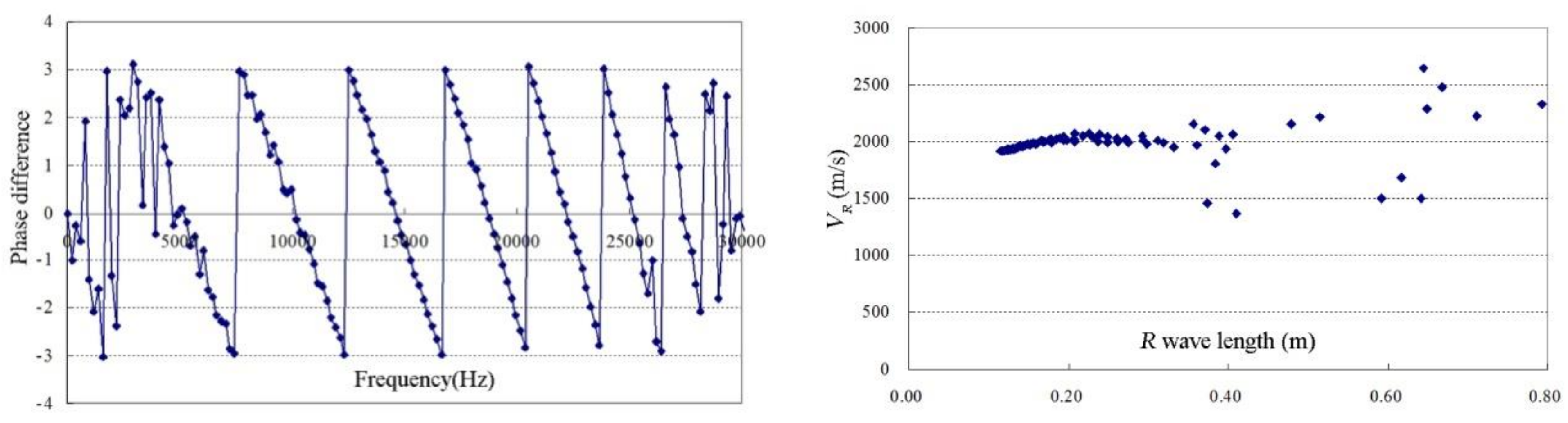
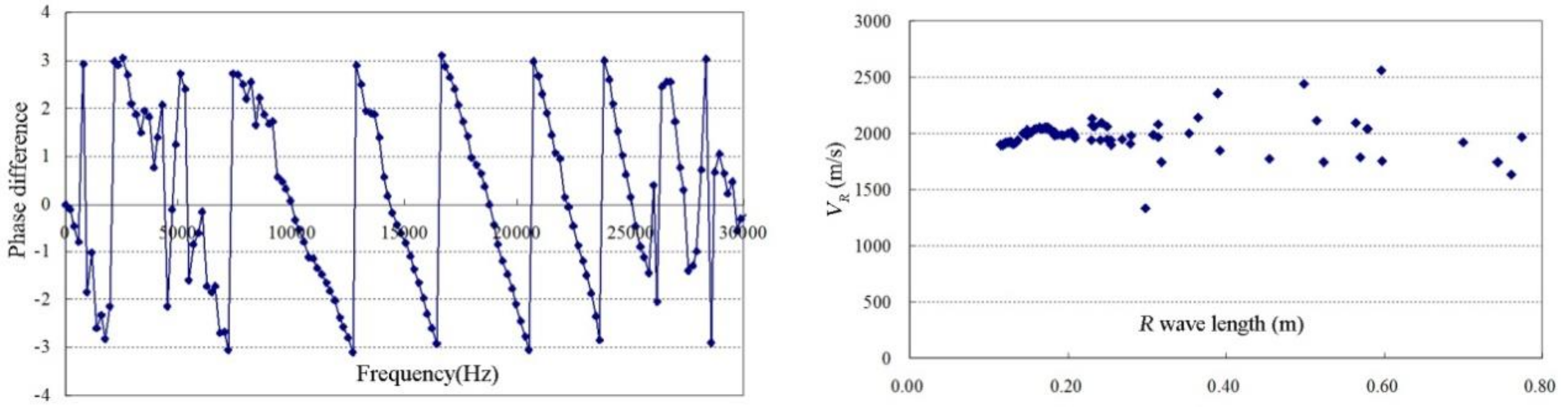
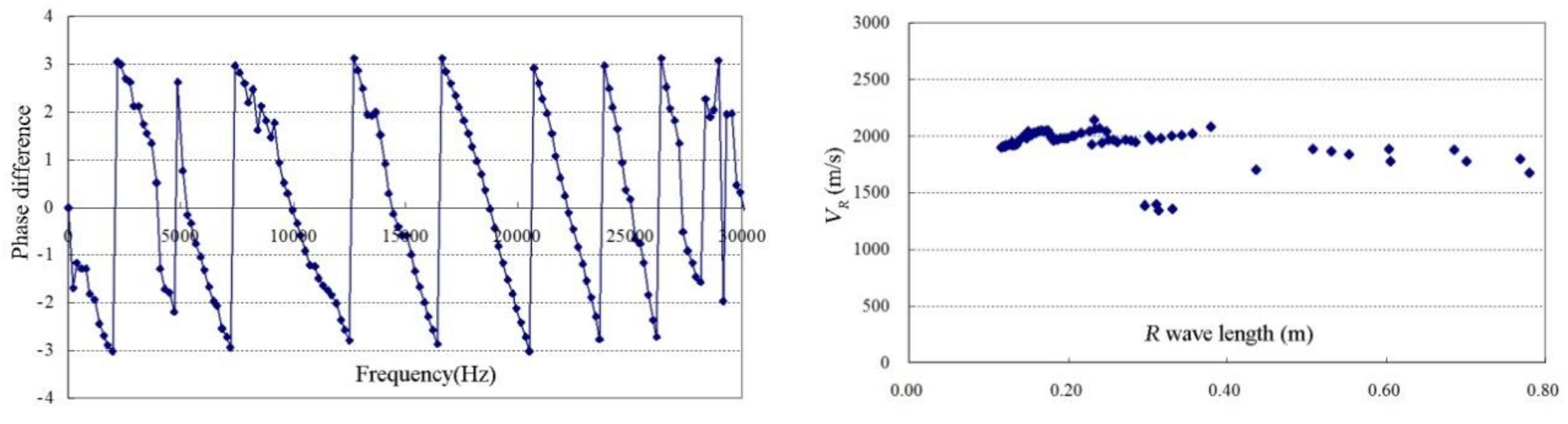
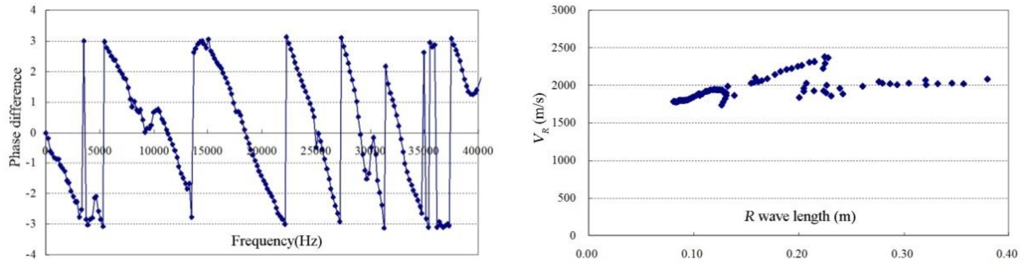
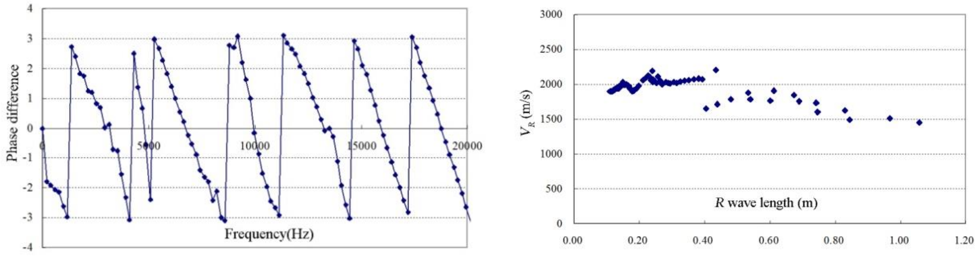
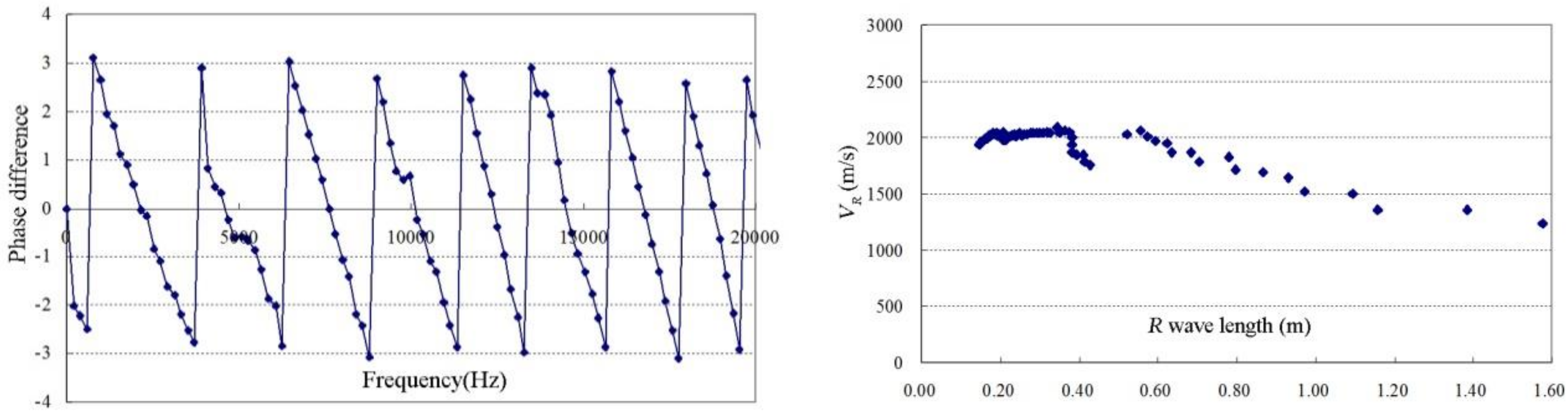
3.1. Dispersion Curves of Different Models

For this part of the study, the nearest offset (i.e., the distance between the impact and the near receiver) was set to 80 cm, and the receiver spacing was 40 cm, which is the same as the thickness of the top concrete layer. The impact duration was set to 250 us, which is roughly the time caused by an instantaneous knock of a typical 30 mm-diameter solid steel ball-hammer at the concrete surface. The purpose was to investigate how different model schemes, both uniform and layered, as shown in Table 2, affect the shapes of phase spectra and dispersion curves.

Figure 6, Figure 7, Figure 8 and Figure 9 show the phase spectra and dispersion curves of the four models. For the uniform model, the phase spectrum shows several repeated cycles, which exhibit a relatively regular and smooth pattern. The first four cycles are quite consistent and have no obvious disturbances. As a result, the R-wave velocity dispersion curve obtained from unwrapping the phase angles on the phase spectrum is generally flat, especially when the R-wave length is larger than 0.2 m, averaging around 2050 m/s, which is quite close to the theoretical value of concrete calculated from Equation (7). It is worth noticing that when the R-wave length is smaller than 0.2 m, the R-wave velocity slightly drops. This can be attributed to the element size effect of the model [17]. It has been shown that the model element size should be less than one-tenth of the shortest R-wave length of interest in order to get a satisfactory analysis result. The element size used in this study is 2 cm; therefore, the R-wave velocity after the R-wave length of 0.2 m tends to be more accurate.

Compared to the uniform model, the first phase cycle at the low frequency of the phase spectrum of the concrete-bedrock model seems to have more interference, thus yielding a more scattered point distribution on the dispersion curve. This scattering starts right from the R-wave length of 40 cm, which coincides with the thickness of the concrete. Except for this scattered portion, the other part of the dispersion curve is almost the same as that of the uniform model.

For the concrete-weak interlayer-bedrock model, unlike the above two, a noticeable discontinuity occurs inside the first cycle of the phase spectrum, generating a more scattered dispersion curve, and the scattering also seems to begin at the R-wave length of 40 cm. For the layered model 3 (concrete-weak layer), the discontinuity inside the first phase cycle becomes more obvious, and this creates an abrupt drop of R-wave velocity at an R-wave length of about 40 cm on the dispersion curve.

It should be noted that for all those four dispersion curves, the R-wave velocity distribution before the R-wave length of 40 cm essentially follows the same trend, and the average (neglecting the element size effect) well approaches the theoretical R-wave velocity of concrete, 2058 m/s.

From Figure 6, Figure 7, Figure 8 and Figure 9, it can be seen that the interface contact condition may be evaluated by inspecting both phase spectra and dispersion curves. When the material properties on both sides of the interface are far-off from each other, like the case of the layered model 3, there will be very clear discontinuities both inside the first phase cycle and on the dispersion curve at the R-wave length roughly equal to the concrete layer thickness. When a weak interface exists between the two layers, which is quite common in the hydraulic tunnel construction, discontinuity will occur in the first phase cycle, but the dispersion curve may not display the abrupt drop of R-wave velocity at the same wave-length as that of the layered model 3.

3.2. Dispersion Curves of Receiver Spacing

The purpose of this part of the study was to find out the influence of different receiver spacings on the efficiency of detecting the existence of a weak layer underneath the concrete using the SASW method. The layered model 3 (concrete-weak layer) was used in this analysis. In addition to the 40 cm spacing discussed above, extra 20 cm, 60 cm, and 80 cm receiver spacings were also introduced. The corresponding nearest offsets were set to be double those of those spacings, while the impact duration was still kept at 250 us.

The analysis results for those three scenarios are shown in Figure 10, Figure 11 and Figure 12. At a receiver spacing of 20 cm, a noticeable disturbance occurs in the first cycle of the phase spectrum, which leads to a discontinuity on the dispersion curve at an R-wave length of about 20 cm, but this is not related to the weak layer underneath, since at this wave length, the R-wave does not penetrate through the 40 cm-thick concrete layer above. In fact, according to the basic rules of SASW, the maximum R-wave length of the dispersion curve is limited to two times that of the receiver spacing. This dispersion curve discontinuity may be caused by the element size effect, as discussed above in Section 3.1.

The phase spectrum and dispersion curve at a receiver spacing of 60 cm in Figure 11 are quite similar to those at a receiver spacing of 40 cm in Figure 9, except that the discontinuity on the phase spectrum moves towards the end of the first phase cycle. However, as shown in Figure 12, at a receiver spacing of 80 cm, the phase spectrum is distinct from those of 40 cm and 60 cm receiver spacings. The phase cycles are seemingly smooth and no apparent discontinuity or interference occurs, and the shape of the dispersion curse is also a little dissimilar. Although there is an interruption on the dispersion curve at the wave length near 40 cm, the R-wave velocity seems more likely to decease gradually after that point, rather than exhibiting an abrupt drop, as shown in Figure 9 and Figure 12.

It is found from the results above that in order to clearly identify the weak layer underneath the concrete slab using the SASW method, the receiver spacing should be set to within the range of 1 to 1.5 times of the slab thickness.

3.3. Dispersion Curves of Impact Duration

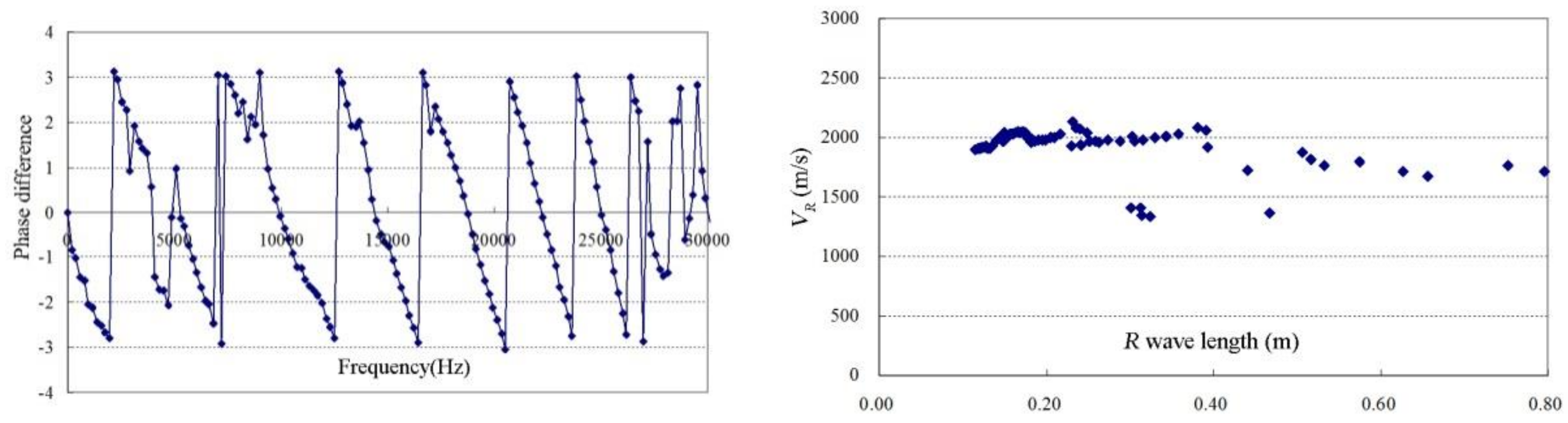
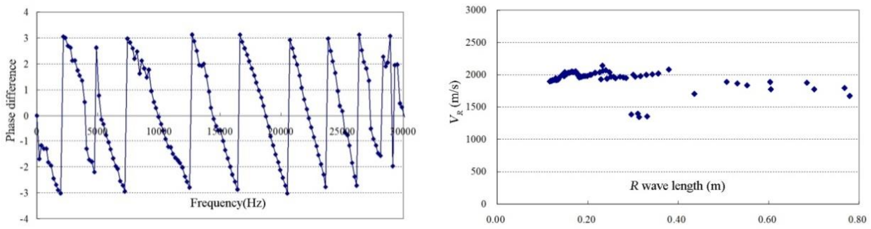
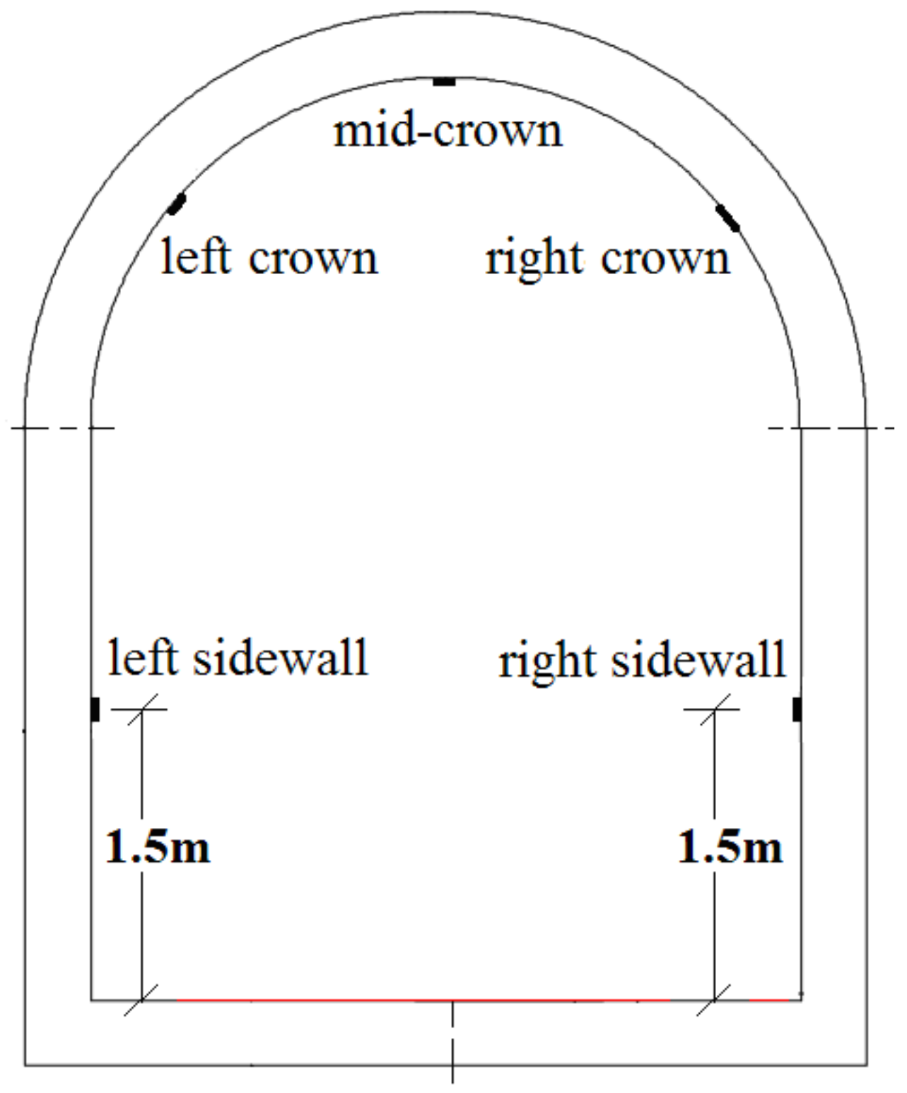
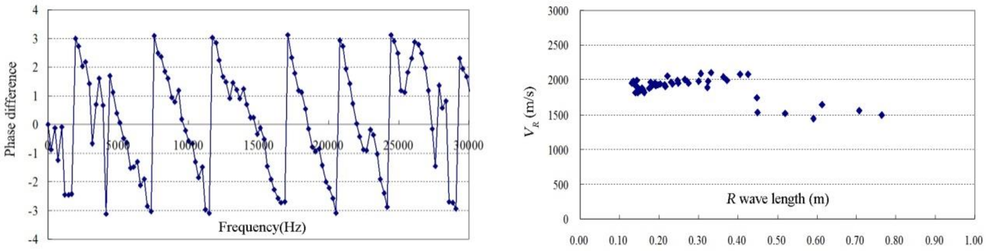
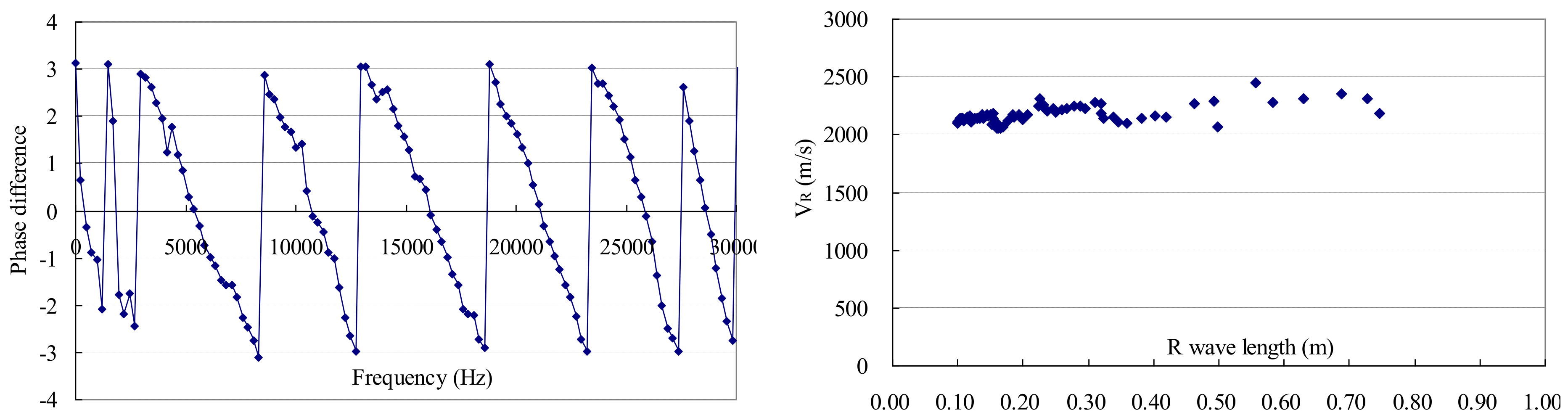
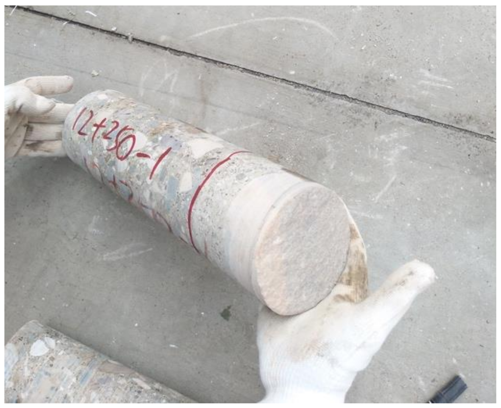
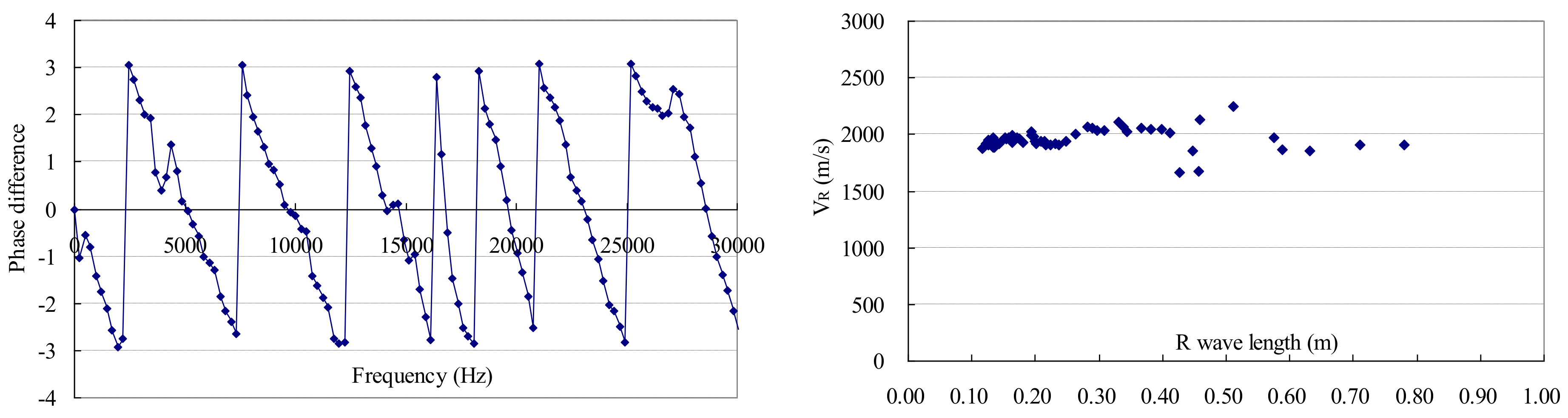
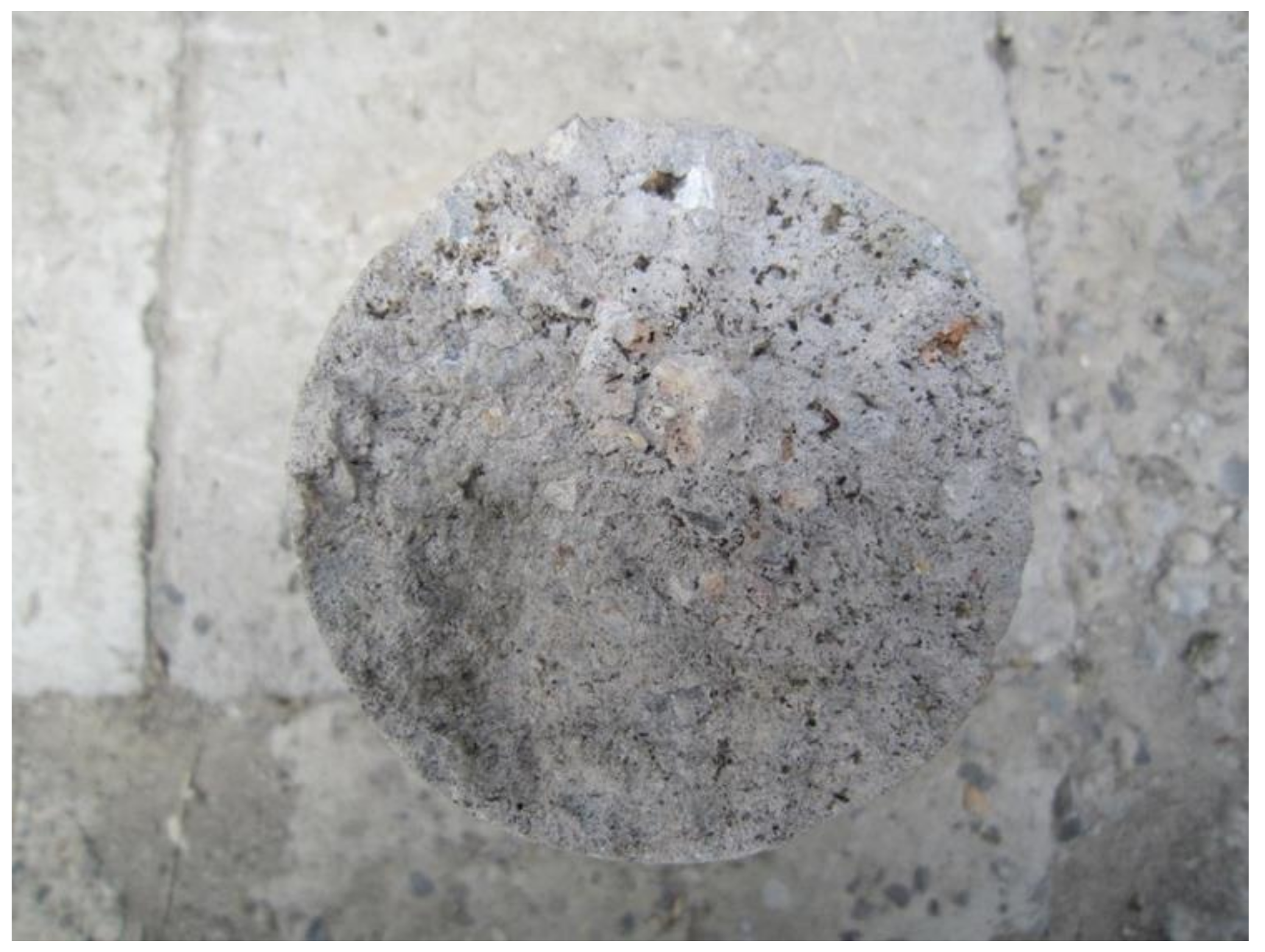
The frequency content of the elastic wave caused by an instantaneous impact on concrete depends on the impact duration of the hammer with the surface. The shorter the impact duration is, the higher the main frequency components will be. Under the same conditions, the bigger the diameter of the solid steel ball-hammer, the longer the impact duration. As stated before, the impact duration from a 30 mm-diameter solid steel ball-hammer at the concrete surface is roughly 250 us. Using the layered model 3 (concrete-weak layer), under a receiver spacing of 40 cm, the effects of impact durations of 100 us and 500 us are also studied, and the results are shown in Figure 13 and Figure 14.

Comparing Figure 9, Figure 13 and Figure 14, it can be seen that, under a certain reasonable range, the impact duration has an insignificant effect on the phase spectra and dispersion curves of a concrete-weak layer model.

3.4. Field Test

In order to verify the applicability of the SASW method, on-site inspection experiments were carried out on the basis of simulation calculations. A conveyance tunnel which diverts water from the Yellow River in Western China will not be put into operation until the lining has passed the quality inspection. The tunnel has a total length of 4.3 km with an arched-gate cross section, of which the width is 4.84 m, the height of its vertical wall is 3.5 m, and the crown radius is 2.42 m. The lining of the tunnel is constructed with C25 concrete with a doubly reinforced section and the steel protective cover is 35 mm thick. The lining thickness of the surrounding rock of Class III, IV, and V is 300 mm, 350 mm, and 400 mm, respectively.

Due to the dense interior and exterior reinforcement of the concrete lining section, the steel bars strongly interfere with the GPR signal and the contact condition at the lining-rock interface cannot be read from the radar image with confidence. The SASW method is then introduced for further investigation. The schematic layout of SASW test stations at each test section is shown in Figure 15. As per the owner’s request, a total of 10 test sections were arranged along the tunnel, of which the locations were chosen based on the GPR results, bedrock types, and apparent concrete quality.

The nearest offset (i.e., distance between the impact point and the nearest transducer) is 40 mm, and the receiver spacing is 80 cm. The sampling interval is 4 us, the sampling points are 1024, and at each station, the impact test is performed four times. The typical phase spectrum and dispersion curve obtained from a mid-crown station at section 11+250 are shown in Figure 16. There are five regular and complete phase cycles in the phase spectrum, among which the first cycle has some strong interference. In the dispersion curve, when the R-wave length is below 40 cm, the R-wave velocity is around 2000 m/s, which reflects the overall quality of the concrete lining, but then a sharp drop to roughly 1500 m/s occurs at the R-wave length of 40 cm. These two irregularities are in good agreement with the results of finite element model analysis, indicating a quite probable void at the concrete-rock interface of the lining crown.

Due to the gravity effect of the flowable concrete mixture during placement at the crown part of the lining and over-excavation, it is very easy for voids to form between the lining and bedrock above, and therefore most of the results of crown test stations, especially the mid-crown ones, have the same pattern as that in Figure 16. The voids could be easily detected by dry-drilling (since it is hard to core at the mid-crown).

For the same reason, it is quite logical to imagine that the concrete-bedrock contact condition should be much better at both sidewall parts. The typical phase spectrum and dispersion curve obtained from the left sidewall station at section 12+250 are shown in Figure 17. The phase cycles exhibit a smooth and regular pattern and no obvious disturbance occurs, which leads to an essentially flat dispersion curve with the R-wave velocity fluctuating near 2200 m/s, indicating good concrete quality and concrete-bedrock connection. This was verified by coring, as shown in Figure 18.

However, there are some sidewall stations where the phase cycles of the phase spectra exhibit some disturbances. As shown by the results of the right sidewall station at section 13+400 in Figure 19, a small but noticeable discontinuity occurs at the first phase cycle, causing scattering on the dispersion curve near the wave length of 40 cm, which is also the lining thickness at that location. As verified by coring, this happens due to insufficient treatment of the excavated rock surface, usually loose sand particles or weak mortar, which forms a weak interlayer between the concrete and bedrock. This weak interlayer is normally porous, low in strength, and easily breaks during coring (see Figure 20).

4. Conclusions

Due to the effect of reinforcing bars on the transmission of the electromagnetic wave of GPR, the on-site inspection of the contact condition between the concrete lining and surrounding rock for hydraulic tunnels often cannot provide accurate results. In this paper, the SASW method is used as an alternative to perform this evaluation task, and the following conclusions are obtained.

(1)

The finite element analysis results of different uniform or layered models show that the SASW method can accurately identify the interface contact condition between the concrete lining and bedrock, especially the existence of voids.

(2)

When the receiver spacing is 1.0–1.5 times that of the thickness of the target object to be inspected, the quality of the collected signal data is the best, which is conducive to improving the accuracy of defect identification.

(3)

Under a certain reasonable range, the impact duration has an insignificant effect on the phase spectra and dispersion curves of a concrete-weak layer model.

(4)

The results of the in-situ SASW inspection are consistent with those of the finite element model analysis, which can accurately tell whether the voids exist at the concrete-bedrock interface. It shows the SASW method may be applied as an effective supplement to the ground penetrating radar in inspecting the densely reinforced concrete tunnels.

(5)

The data processing program of the SASW method based on the MATLAB platform is accurate, convenient, and worth promoting.

References

1. Goodman, D. Ground-penetrating radar simulation in engineering and archaeology. Geophysics 1994, 59, 224–232. [Google Scholar] [CrossRef]
2. Annan, A.P. The history of ground penetrating radar. Subsurf. Sens. Technol. Appl. 2002, 3, 303–320. [Google Scholar] [CrossRef]
3. Fisher, E.; Mcmechan, G.A.; Annan, A.P.; Cosway, S.W. Examples of reverse-time migration of single-channel, ground-penetrating radar profiles. Geophysics 1992, 57, 577–586. [Google Scholar] [CrossRef]
4. Kohler, B.; Schubert, F. Study of Impact Excited Elastic Waves in Concrete by Scanning Laser Vibrometry. Quant. Nondestruct. Eval. 2006, 820, 1328–1334. [Google Scholar] [CrossRef]
5. Wieczorek, G.F.; Snyder, J.B.; Waitt, R.B.; Morrissey, M.M.; Uhrhammer, R.A.; Harp, E.L.; Norris, R.D.; Bursik, M.I.; Finewood, L.G. Unusual July 10, 1996, rock fall at happy isles, Yosemite National Park, California. Geol. Soc. Am. Bull. 2000, 112, 75–85. [Google Scholar] [CrossRef]
6. Mutlib, N.K.; Baharom, S.; Nuawi, M.Z.; El-Shafie, A. Ultrasonic surface wave monitoring for steel fibre-reinforced concrete using gel-coupled piezoceramic sensors: A case study. Arab. J. Sci. Eng. 2016, 41, 1–9. [Google Scholar] [CrossRef]
7. Karaman, K.; Kesimal, A. Correlation of schmidt rebound hardness with uniaxial compressive strength and p-wave velocity of rock materials. Arab. J. Sci. Eng. 2015, 40, 1897–1906. [Google Scholar] [CrossRef]
8. Hawwa, M.A. Shear waves in an initially stressed elastic plate with periodic corrugations. Arab. J. Sci. Eng. 2016, 42, 1–10. [Google Scholar] [CrossRef]
9. Olson, L.D.; Miller, P. Comparison of Surface Wave Tests for Pavement System Thicknesses/Moduli. In Proceedings of the GeoHunan International Conference: Challenges and Recent Advances in Pavement Technologies and Transportation Geotechnics, Changsha, China, 3–6 August 2009; Volume 189, pp. 174–179. [Google Scholar]
10. Ismail, M.A.; Samsudin, A.R.; Rafek, A.G.; Nayan, K.A.M. In Situ Determination of Layer Thickness and Elastic Moduli of Asphalt Pavement Systems by Spectral Analysis of Surface Waves (SASW) Method. In Proceedings of the GeoHunan International Conference: Challenges and Recent Advances in Pavement Technologies and Transportation Geotechnics, Changsha, China, 3–6 August 2009. [Google Scholar]
11. Cho, Y.S. Ndt response of spectral analysis of surface wave method to multi-layer thin high-strength concrete structures. Ultrasonics 2002, 40, 227–230. [Google Scholar] [CrossRef]
12. Barkan, D.D.; Drashevska, L. Dynamics of Bases and Foundations; McGraw-Hill Book Company Inc.: New York, NY, USA, 1962. [Google Scholar]
13. Volti, T.; Burbidge, D.; Collins, C.; Asten, M.; Odum, J.; Pascal, C.H.; Holzschuh, J. Comparisons between vs30 and spectral response for 30 sites in Newcastle, Australia, from collocated seismic cone penetrometer, active- and passive-source vs. data comparisons between vs30 and spectral response for 30 sites in Australia. Bull. Seismol. Soc. Am. 2016, 106, 1690–1709. [Google Scholar] [CrossRef]
14. Lu, Y.; Cao, Y.; Mcdaniel, J.G.; Wang, M.L. Fast Inversion of Air-Coupled Spectral Analysis of Surface Wave (SASW) Using in situ Particle Displacement. ISPRS Int. J. Geo-Inf. 2015, 4, 2619–2637. [Google Scholar] [CrossRef] [Green Version]
15. Nazarian, S.; Stoke, K.H., II. In-Situ Determination of Elastic Moduli of Pavements Systems by Spectral Analysis of Surface Waves Method (Practical Aspects); Research Report Number 368-1F; US Department of Transportation, Federal Highway Administration: Washington, DC, USA, 1985. [Google Scholar]
16. Kim, D.S.; Seo, W.S.; Lee, K.M. IE–SASW method for nondestructive evaluation of concrete structure. NDT E Int. 2006, 39, 143–154. [Google Scholar] [CrossRef]
17. Lu, X.; Sun, Q.; Feng, W.; Tian, J. Evaluation of dynamic modulus of elasticity of concrete using impact-echo method. Constr. Build. Mater. 2013, 47, 231–239. [Google Scholar] [CrossRef]
18. Ma, F.; Wang, R.; Lu, X.; Luke, A. Assessing frost resistance of concrete by impact-echo method. Mag. Concr. Res. 2015, 67, 1–8. [Google Scholar]
19. Kang, S.L.; Choi, J.I.; Kim, S.K.; Lee, B.K.; Hwang, J.S.; Bang, Y.L. Damping and mechanical properties of composite composed of polyurethane matrix and preplaced aggregates. Constr. Build. Mater. 2017, 145, 68–75. [Google Scholar] [CrossRef]
20. Kim, D.S.; Kim, H.W.; Seo, W.S.; Choi, K.C.; Woo, S.K. Feasibility study of the IE-SASW method for nondestructive evaluation of containment building structures in nuclear power plants. NDT E Int. 2003, 219, 97–110. [Google Scholar] [CrossRef]
21. Chen, Z.S.; Jiang, B.F.; Song, J.J.; Wang, W.T. Accurate Sparse Recovery of Rayleigh Wave Characteristics Using Fast Analysis of Wave Speed (FAWS) Algorithm for Soft Soil Layers. Appl. Sci. 2018, 8, 1204. [Google Scholar] [CrossRef]
22. Harley, J.B.; Moura, J.M. Sparse recovery of the multimodal and dispersive characteristics of lamb waves. J. Acoust. Soc. Am. 2013, 133, 2732–2745. [Google Scholar] [CrossRef] [PubMed]
23. Song, X.; Tang, L.; Lv, X.; Fang, H.; Gu, H. Application of particle swarm optimization to interpret rayleigh wave dispersion curves. J. Appl. Geophys. 2012, 84, 1–13. [Google Scholar] [CrossRef]
24. Snowball, P.S.I. Spectral Analysis of Signals. Leber Magen Darm 2005, 13, 57–63. [Google Scholar]
25. Rao, K.D.; Swamy, M.N.S. Spectral Analysis of Signals. In Digital Signal Processing; Springer Singapore: Cham, Switzerland, 2018. [Google Scholar]
26. Lee, U. Spectral Analysis of Signals. Spectral Element Method in Structural Dynamics; John Wiley & Sons, Ltd.: Hoboken, NJ, USA, 2005; pp. 57–63. [Google Scholar]
27. Singh, A.; Derybel, T.; Marti, J.R. FFT tutor: A matlab-based instructional tool for FFT parameter exploration. Acoust. Week Can. 2008, 36, 82–83. [Google Scholar]
28. Xu, Y.; Zhang, X.M.; Wang, Y.; Sun, Q.B.; Wang, Z.M.; Sun, Y. A new method of spectrum analysis based on DFT. Power Syst. Prot. Control 2011, 39, 38–43. [Google Scholar]
29. Zeng, S.; Shen, H.; Zhen, Y.U. FFT based spectrogram analysis and display of signals using matlab. Bull. Sci. Technol. 2000. [Google Scholar]
30. Lyon, D.A. The Discrete Fourier Transform, Part 6: Cross-Correlation. J. Object Technol. 2010, 9, 17–22. [Google Scholar] [CrossRef]
31. Pei, S.; Ding, J.; Chang, J. Efficient implementation of quaternion Fourier transform, convolution, and correlation by 2-D complex FFT. IEEE Trans. Signal Process. 2001, 49, 2783–2797. [Google Scholar] [CrossRef]
Figure 1. Schematic elastic wave propagation generated by impact excitation [12].
Applsci 08 02428 g001
Figure 2. Schematic layout of the SASW test.
Applsci 08 02428 g002
Figure 3. Matlab implementation procedures of the SASW method.
Applsci 08 02428 g003
Figure 4. Numerical model and schematic layout of impact and receivers.
Applsci 08 02428 g004
Figure 5. Layered model 2 (concrete-weak interlayer-bedrock).
Applsci 08 02428 g005
Figure 6. Phase spectrum and dispersion curve of the uniform model.
Applsci 08 02428 g006
Figure 7. Phase spectrum and dispersion curve of the layered model 1 (concrete-bedrock).
Applsci 08 02428 g007
Figure 8. Phase spectrum and dispersion curve of the layered model 2 (concrete-weak interlayer-bedrock).
Applsci 08 02428 g008
Figure 9. Phase spectrum and dispersion curve of the layered model 3 (concrete-weak layer).
Applsci 08 02428 g009
Figure 10. Phase spectrum and dispersion curve of the layered model 3 @ receiver spacing 20 cm.
Applsci 08 02428 g010
Figure 11. Phase spectrum and dispersion curve of the layered model 3 @ receiver spacing 60 cm.
Applsci 08 02428 g011
Figure 12. Phase spectrum and dispersion curve of the layered model 3 @ receiver spacing 80 cm.
Applsci 08 02428 g012
Figure 13. Phase spectrum and dispersion curve of the layered model 3 @ impact duration 500 us.
Applsci 08 02428 g013
Figure 14. Phase spectrum and dispersion curve of the layered model 3 @ impact duration 100 us.
Applsci 08 02428 g014
Figure 15. Schematic layout of SASW test stations at each test section.
Applsci 08 02428 g015
Figure 16. Phase spectrum and dispersion curve at the mid-crown test station at section 11+250.
Applsci 08 02428 g016
Figure 17. Phase spectrum and dispersion curve at the left sidewall test station at section 12+250.
Applsci 08 02428 g017
Figure 18. Core sample at the left sidewall test station at section 12+250.
Applsci 08 02428 g018
Figure 19. Phase spectrum and dispersion curve at the right sidewall test station at section 13+400.
Applsci 08 02428 g019
Figure 20. Broken weak interlayer between concrete and bedrock.
Applsci 08 02428 g020