5.1. Simulation 1
Most existing stability criteria for trotting gaits assume that the robot is in stable motion only when ZMP is located on the support line formed by the current support feet. However, this is inconsistent with the movement of animals in nature. To illustrate that these stability criteria cannot accurately determine the stability state of the robot, the following simulation was designed.
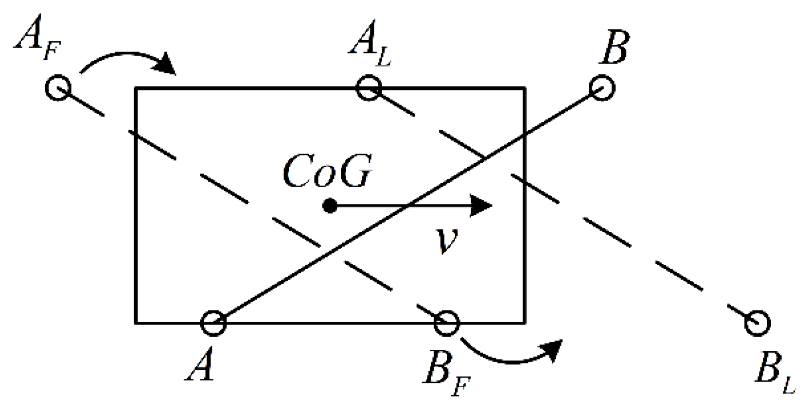
The projection of CoM in the direction of gravity onto the virtual-support plane is denoted by CoG. In the trot-gait-motion planning used in this simulation, the CoM of the body moves forward at a constant speed and, at each phase-changing point, CoG is located at the center of the quadrilateral formed by the just-disappearing support line and the newly formed line (see
Figure 13).
The simulation animation is in
Video S1. The position changes of the support lines, CoG, and
ZMP on the support plane (
plane) during the entire simulation process are shown in
Figure 14.
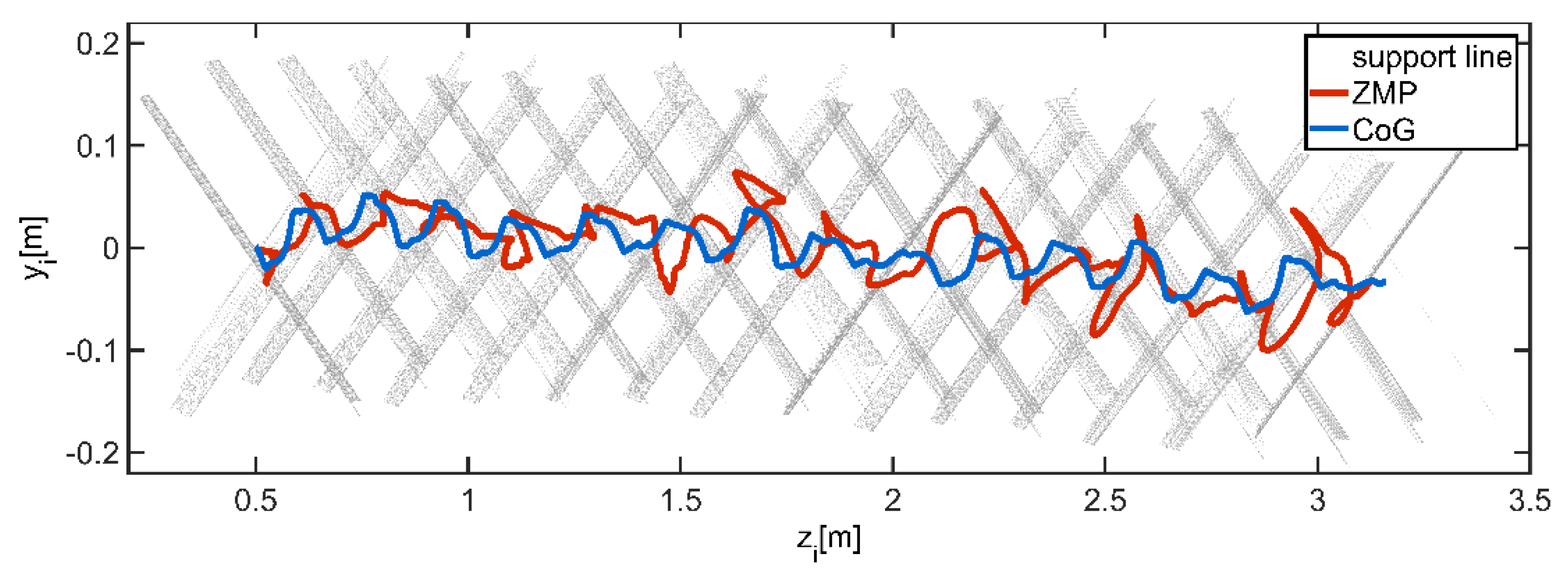
The gray lines in
Figure 14 are the support lines and are shown as several groups of line clusters for two reasons. First, the active or passive compliance was not considered in this simulation process, therefore the feet were bouncing for a short period after landing. Second, the feet were slipping during the support phases. The blue line is the actual motion trajectory of CoG on the horizontal plane. The motion trajectory of CoG was not completely consistent with the planned trajectory under the influence of the unbalanced moment around the current support line, the legs’ movement, and the impact force at the feet. The red line is the trajectory of traditional
ZMP. It can be clearly seen that, during this simulation,
ZMP was not always or mostly located on the current support line.
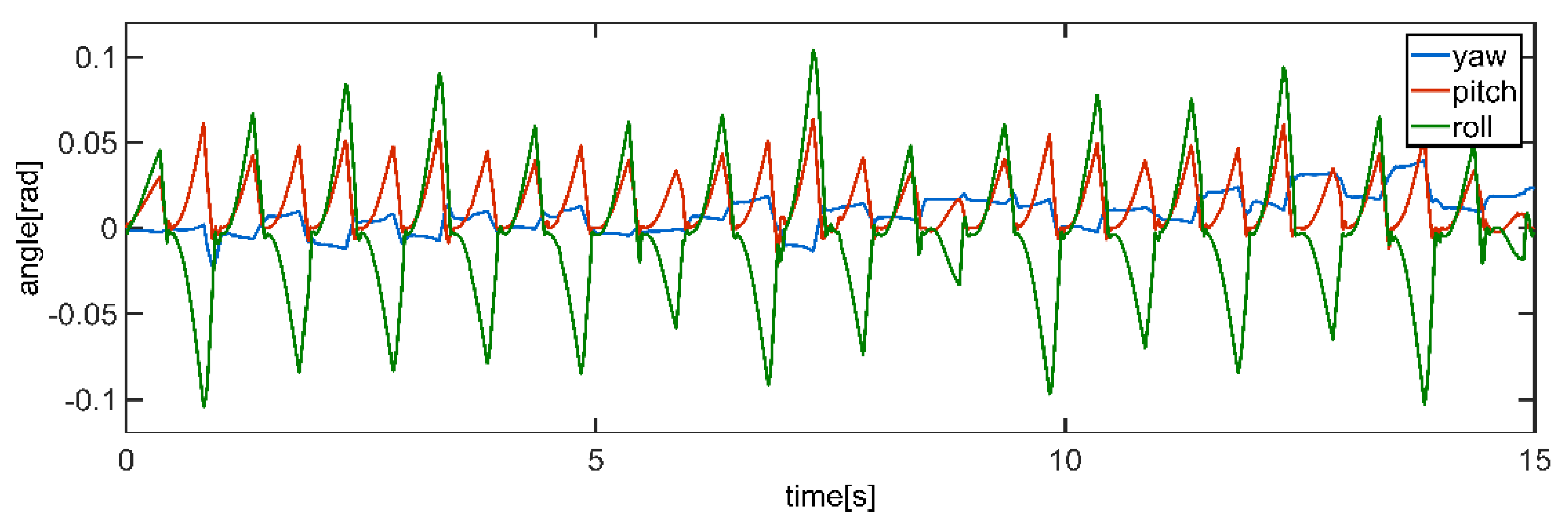
As shown in
Figure 15, the running direction of the body was slightly skewed (see yaw angle), and the absolute values of the pitch and roll angles were less than 0.11 rad (6°). The curves of these attitude angles show that the robot moved stably and had no obvious tendency to tumble. This indicates that the existing stability criteria for the trot gait cannot accurately determine the stability state of the robot.
5.2. Simulation 2
A second set of comparative simulations was designed to verify the following: (1) it is difficult to correctly evaluate the stability by only considering the distance between
ZMP and the current support line; (2) the accuracy and effectivity of LAR are worse than the stability-evaluation method proposed in this paper; and (3) the stability-evaluation method proposed in this paper can satisfy the first two requirements of a good-stability criterion and evaluation method presented in
Section 1.
In addition to the motion trajectory of the CoG used in Simulation 1 (denoted as Test 1), two other CoG trajectories were used for off-line planning of the quadruped robot’s movement (the actual trajectories of CoG did not necessarily coincide with the planned trajectory); refer to the animation (
Video S2).
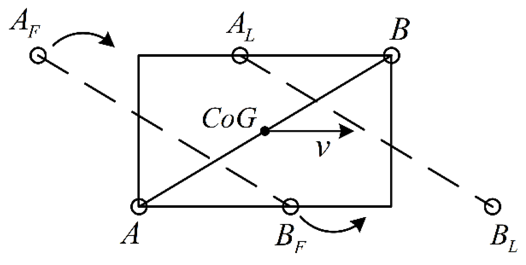
Test 2: CoG moves around the current support line (the velocity parallel to
is 0.2 m/s, and the velocity and acceleration parallel to
at the two ends of this direction are zero), as shown in
Figure 16.
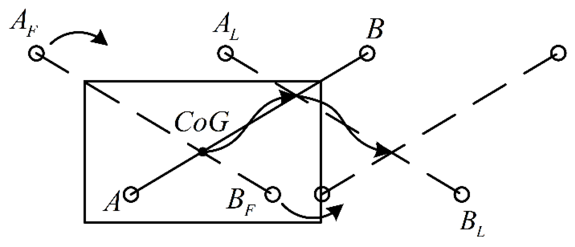
Test 3: CoG starts to move from the midpoint of the current support line to that of the next support line at a constant speed when the previous support line has just disappeared, as shown in
Figure 17.
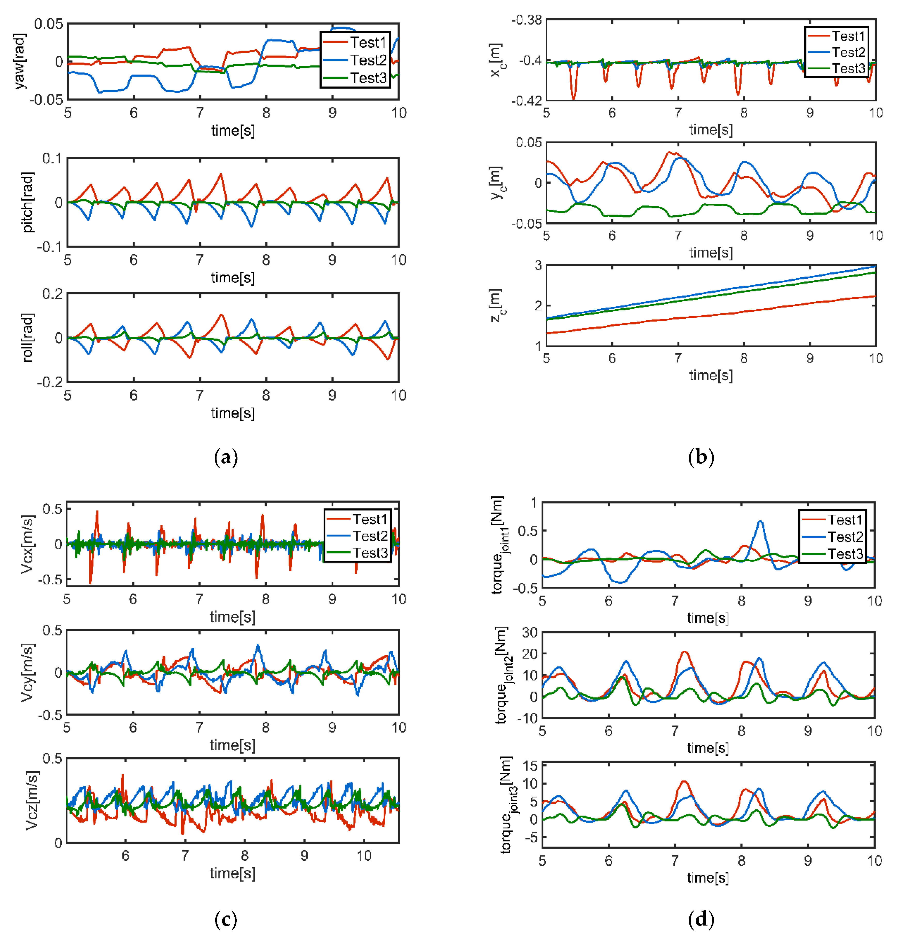
The posture angles, positions, and velocities of the body for the three tests are shown in
Figure 18a–c, respectively. The driving moments of the three joints of the left hind leg are shown in
Figure 18d.
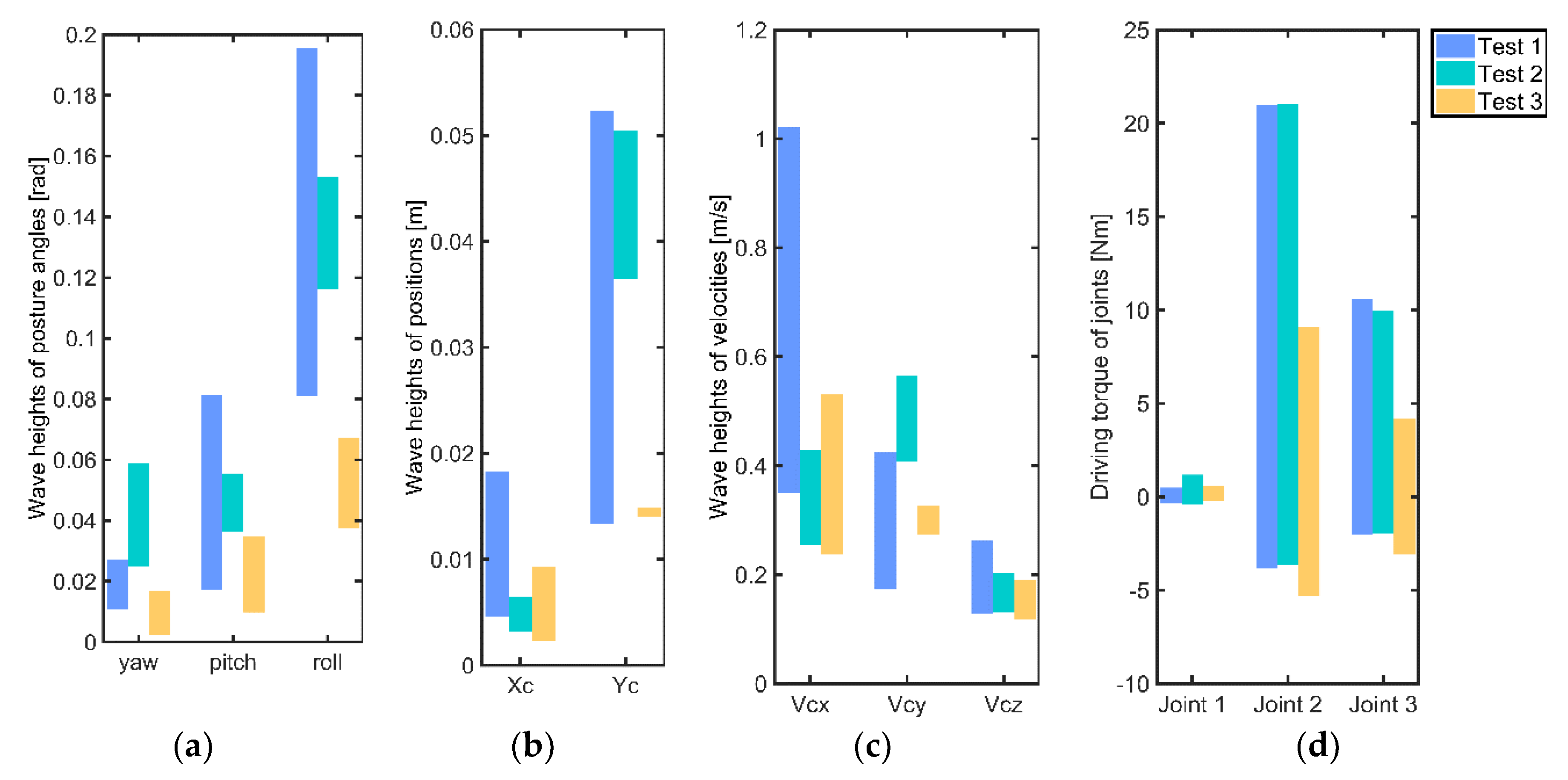
The wave heights of the data curves referring to the difference between adjacent peaks and troughs show the severity of data fluctuations if the fluctuation period is similar. The wave-height-variation range of each dataset and the driving-torque-variation ranges of the three joints of the left hind leg are shown in
Figure 19.
As shown in
Figure 19, the motion of Test 3 was the steadiest and required the minimum joint-driving torque, and the stabilities of the other two tests were about the same. In fact, stability cannot be evaluated accurately using individual-sensor data, which is one of the reasons the stability criterion and measurement must be proposed.
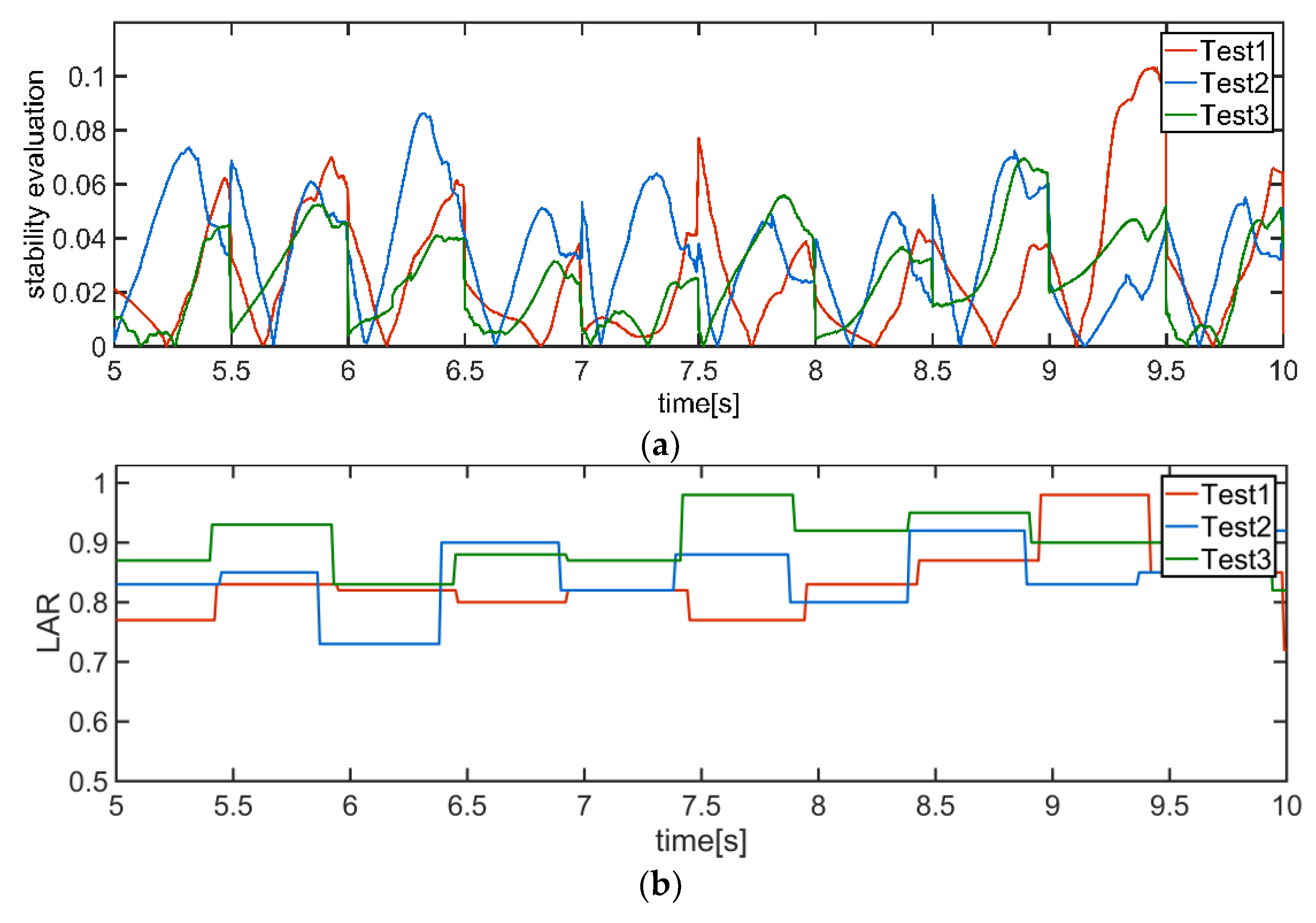
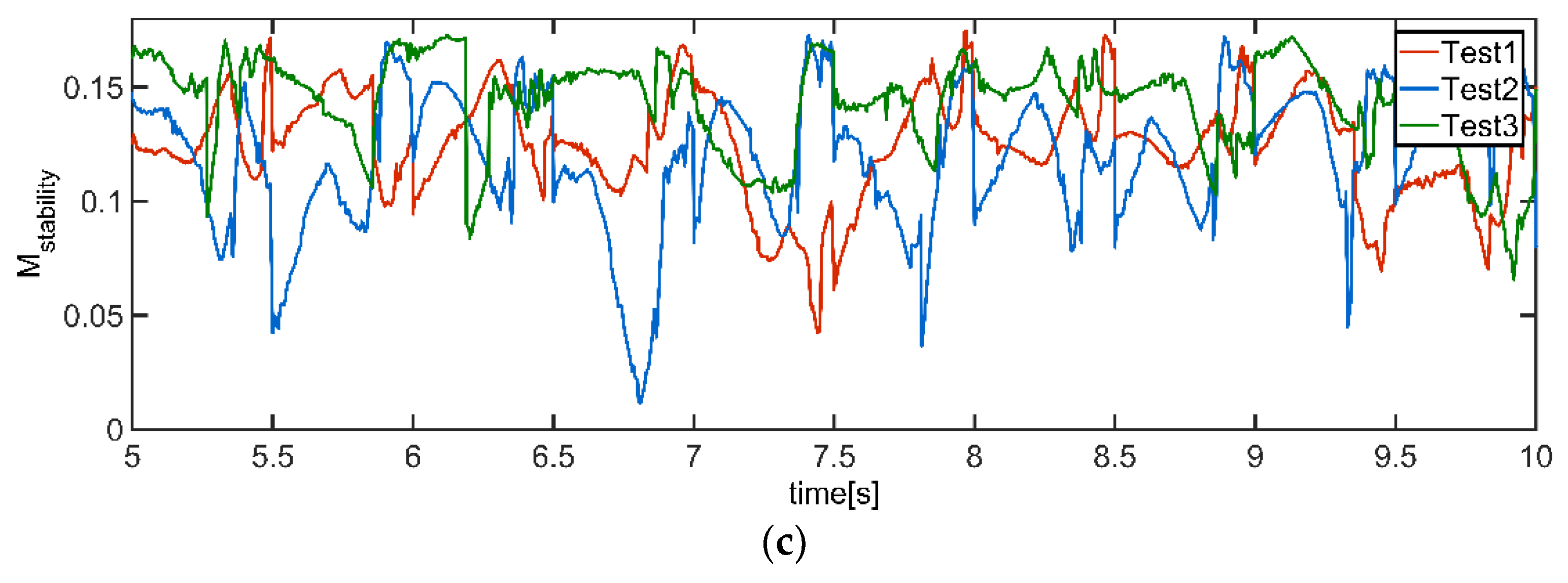
The generally accepted stability-evaluation method (denoted as Method 1), i.e., the one that measures the distance between the traditional
ZMP and the current support line; LAR (denoted as Method 2); and the proposed stability measurement for the trot gait of a quadruped robot (denoted as Method 3) were used to evaluate the stability of the three tests (
Figure 20a–c).
The average values (over 15 s) of the stability evaluations obtained using these three methods are shown in
Table 4.
Test 2 had the lowest stability, followed by Test 3 and then Test 1 according to Method 1. However, this result was not consistent with the actual movement of the robot. Method 2 indicated that the stability of the robot in Test 3 was better than Test 2, followed by Test 1. Using the second method, the stability of Test 1 was found to be slightly better than that of Test 2, with Test 3 being the most stable case. The last two methods could both indicate that the stability of Test 3 was best, but one more simulation should be designed to compare the stability of Test 1 and Test 2.
Two impact forces parallel to
in the opposite direction were both applied to the CoM of the body during the trotting in Test 1 and Test 2. The magnitudes, timings, and durations of these forces are shown in
Table 5.
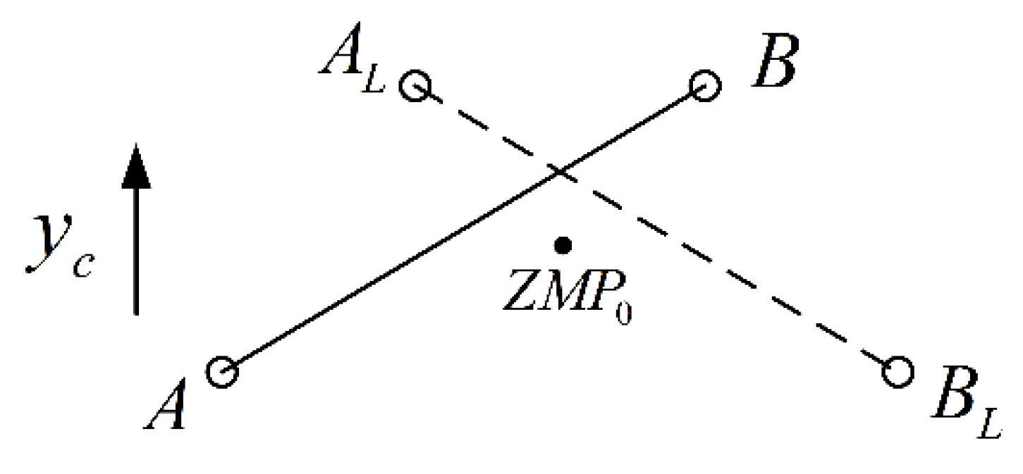
The robot is supported by the same set of diagonal legs during the first half of each gait cycle of the trotting gait. The magnitude of the forces that the robot can bear differs in the positive and negative directions of if the positions of and the next support line are fixed.
For example, in the case shown in
Figure 21, the impact forces in the positive and negative directions of
can both drive
ZMP0 closer to the boundaries of the virtual-support quadrilateral. However, the force in the positive direction can reduce the distance between
ZMP and the support lines, whereas the force in the negative direction increases this distance. Thus, the robot can endure a greater positive impact force along
.
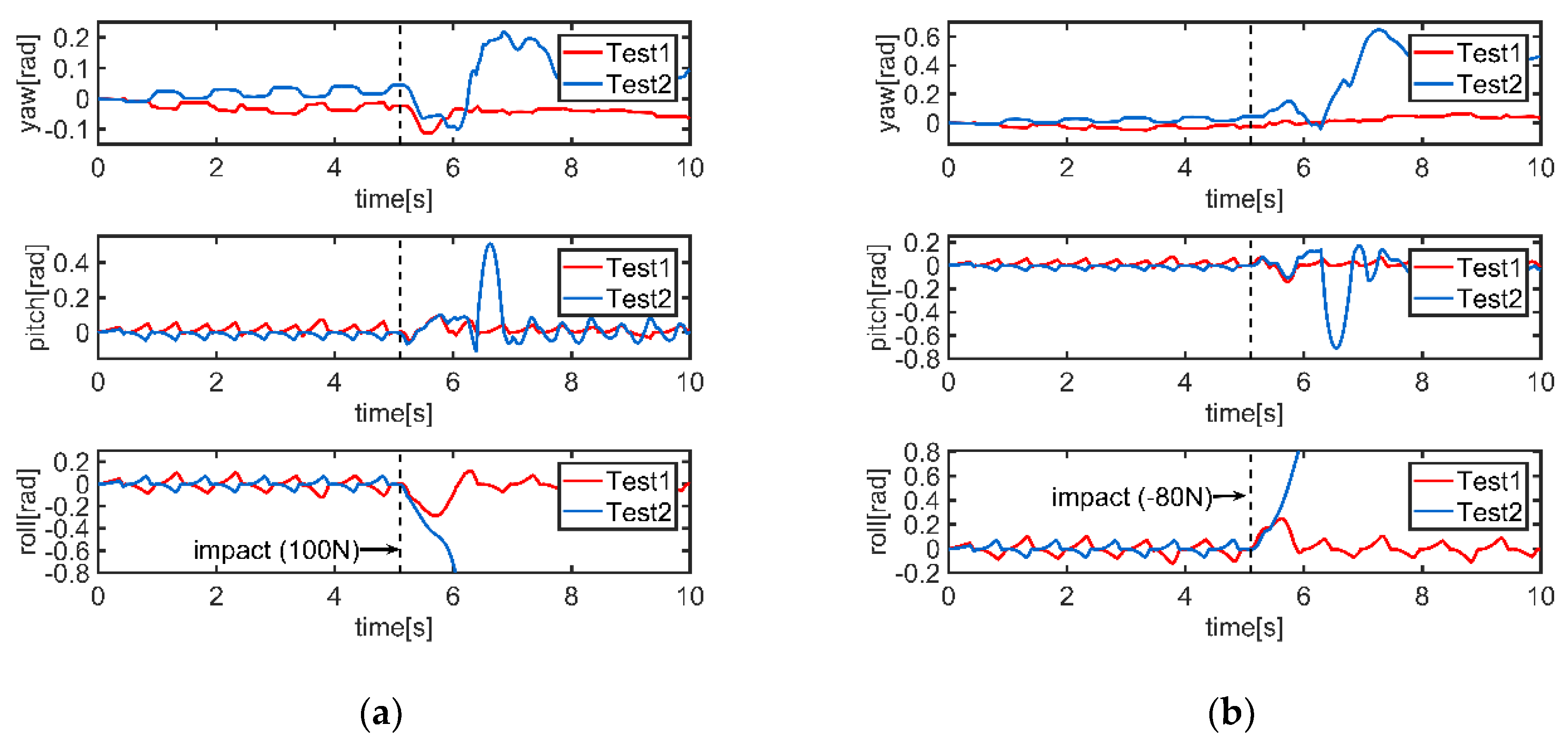
The changes of the posture angles of these two tests under impacts are shown in
Figure 22.
The robot in Test 2 tumbled to the ground after those two impact forces acting in different directions, while the robot in Test 3 could sustain the impacts without losing its stability. This means that the stability of the motion in Test 1 was better than Test 2, thus the method proposed in this paper could evaluate the stability of the quadruped robot with trotting gait more accurately than LAR.
Three impact forces parallel to
were applied to the CoM of the body in the three trotting tests, as described above, to further illustrate the accuracy of the proposed stability criterion and measurement. The magnitudes, timings, and durations of these forces are shown in
Table 6.
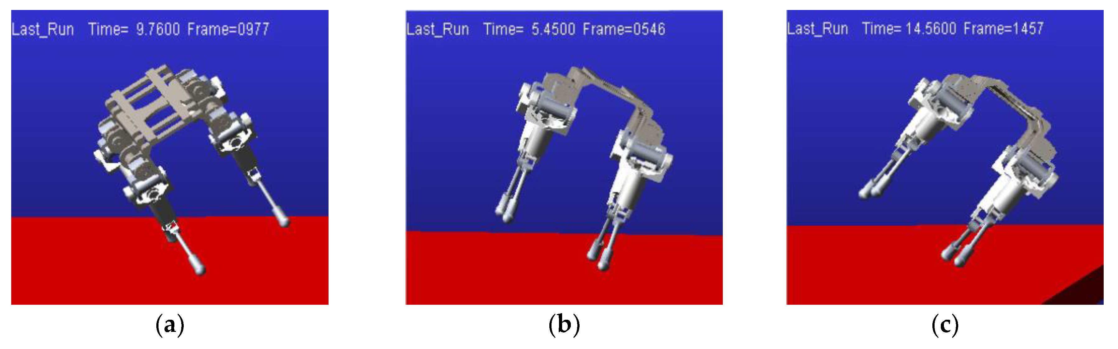
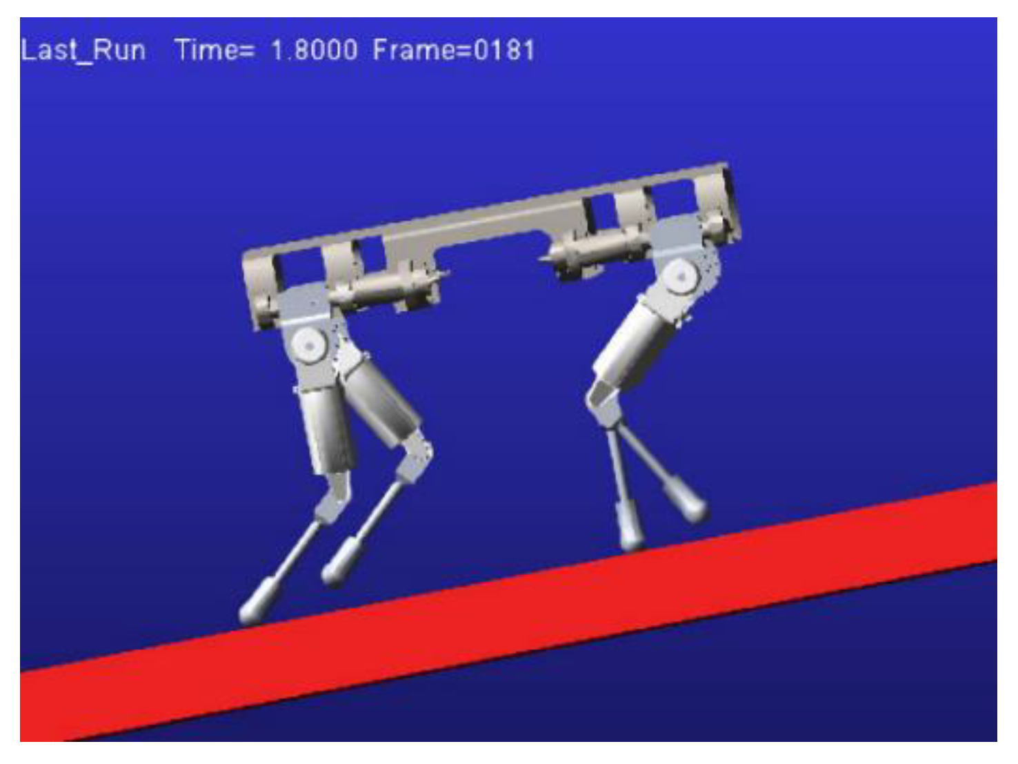
The simulation results of these three tests after impacts are shown in
Figure 23.
Test 2 was the least able to bear the impact force in the positive direction of
, since the positions of the next set of support feet differed with respect to
ZMP0 (as can be seen simply from the positions of the next support lines with respect to CoG), tumbling after the first impact (
Figure 23b). The robot walked stably in Test 1 until the second impact was applied to the body (
Figure 23a), and the robot in Test 3 lost its balance after the last impact (
Figure 23c).
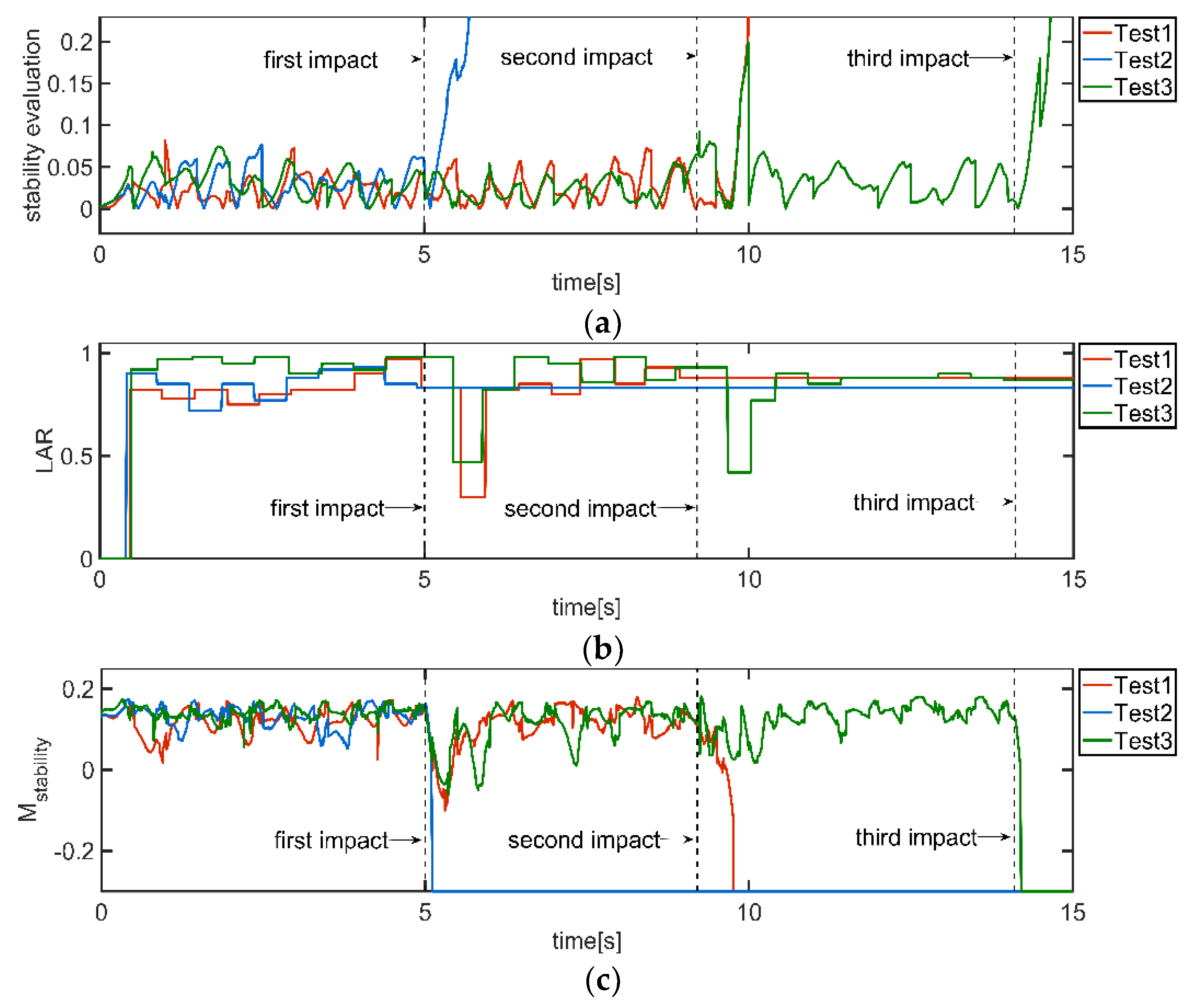
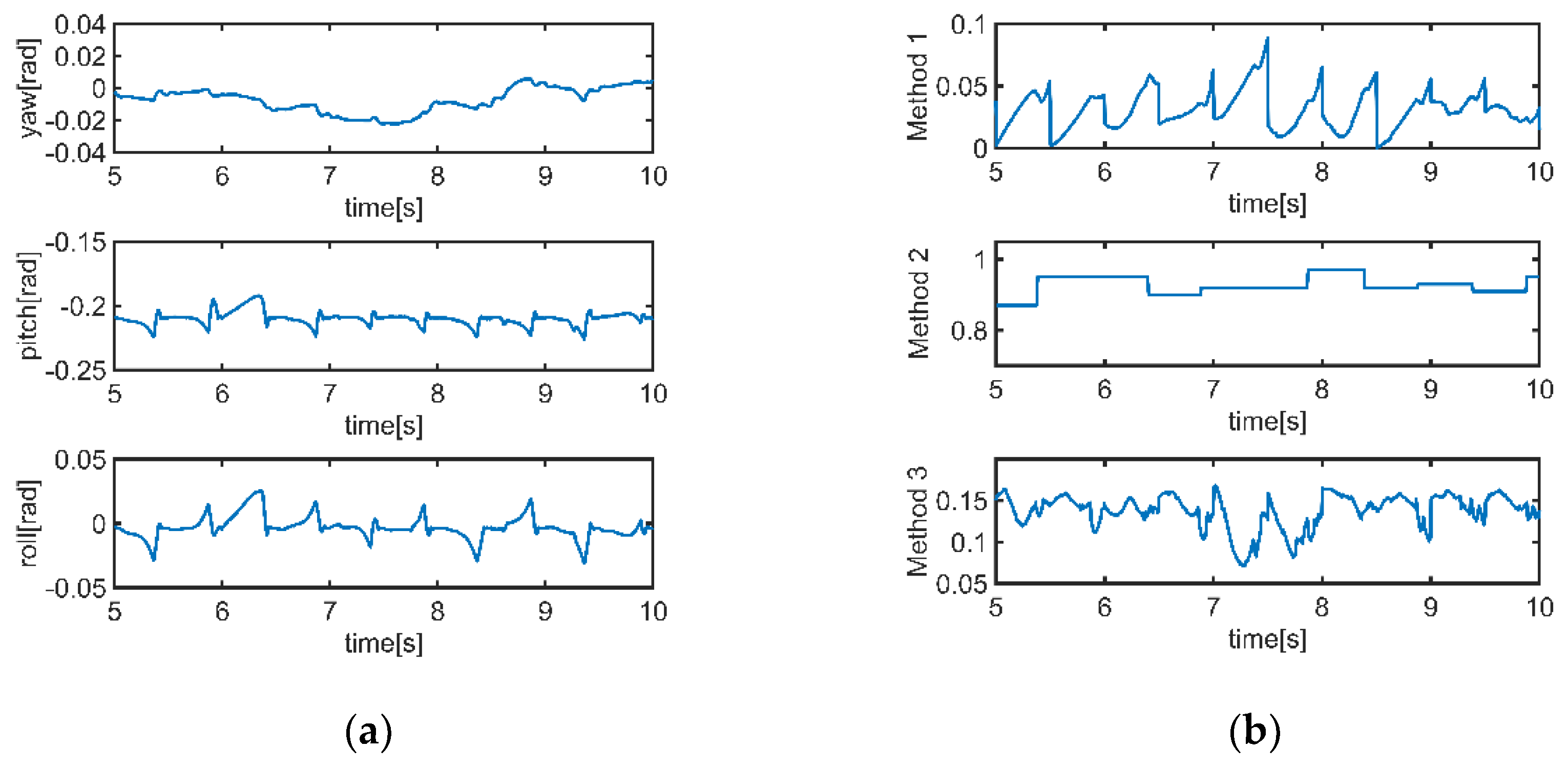
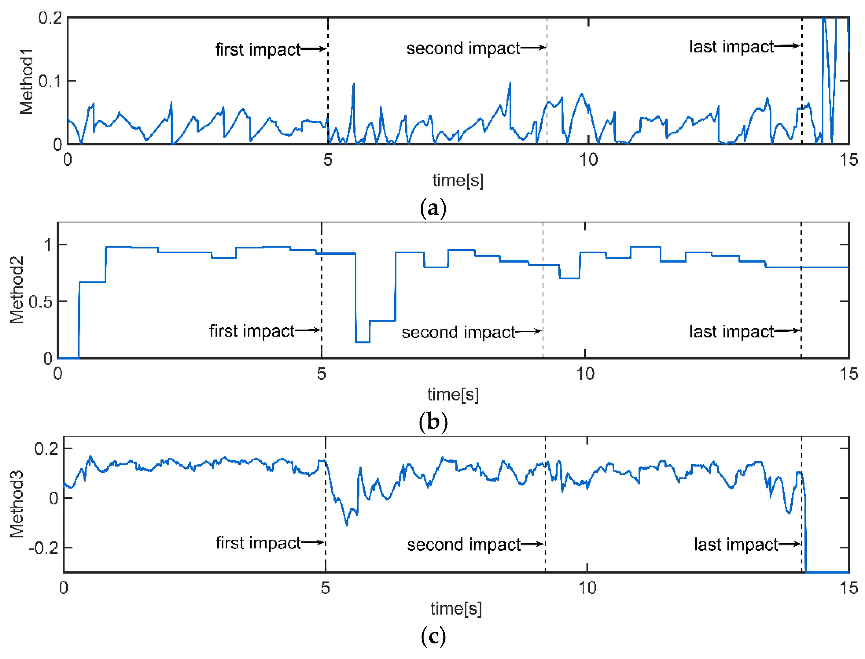
The three stability-evaluation methods were also used for the analysis of the three tests with external impacts. To illustrate this intuitively, for Method 2, the stability measurement was set to −0.3 if ZMP0 was outside the virtual-support quadrilateral and the robot lost its balance according to Equation (40).
As shown in
Figure 24, the distance between
ZMP and the current support line was not zero for most of the time, making it very difficult to determine when the robot would lose its balance. Using Method 2, it was hard to decide when to update the value of LAR if the robot tips over, because one of the feet would never touch the ground. From the results of Method 3, the robot was considered to lose its balance at 9.753 s (Test 1), 5.109 s (Test 2), and 14.2 s (Test 3), which was consistent with the actual motions of the robot.
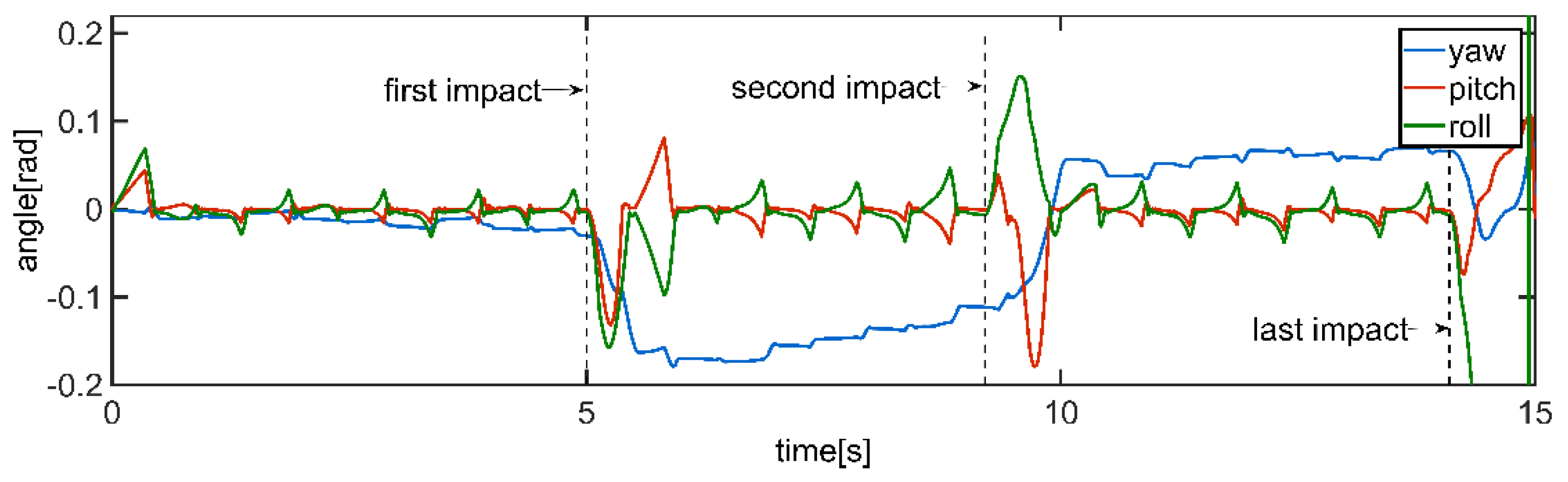
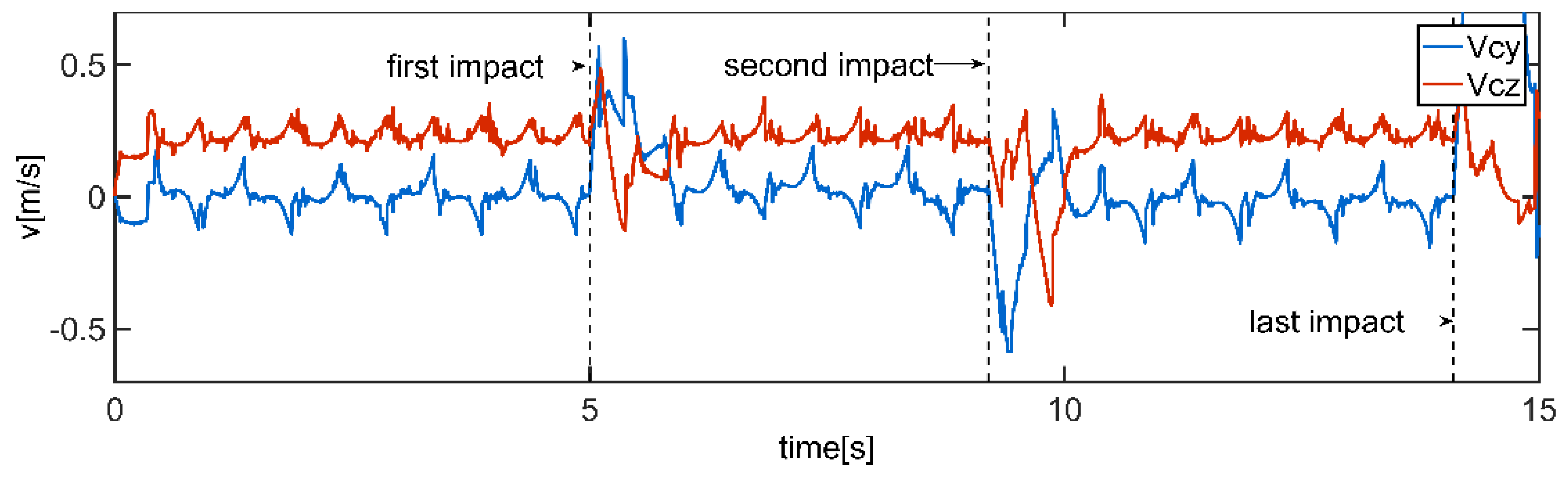
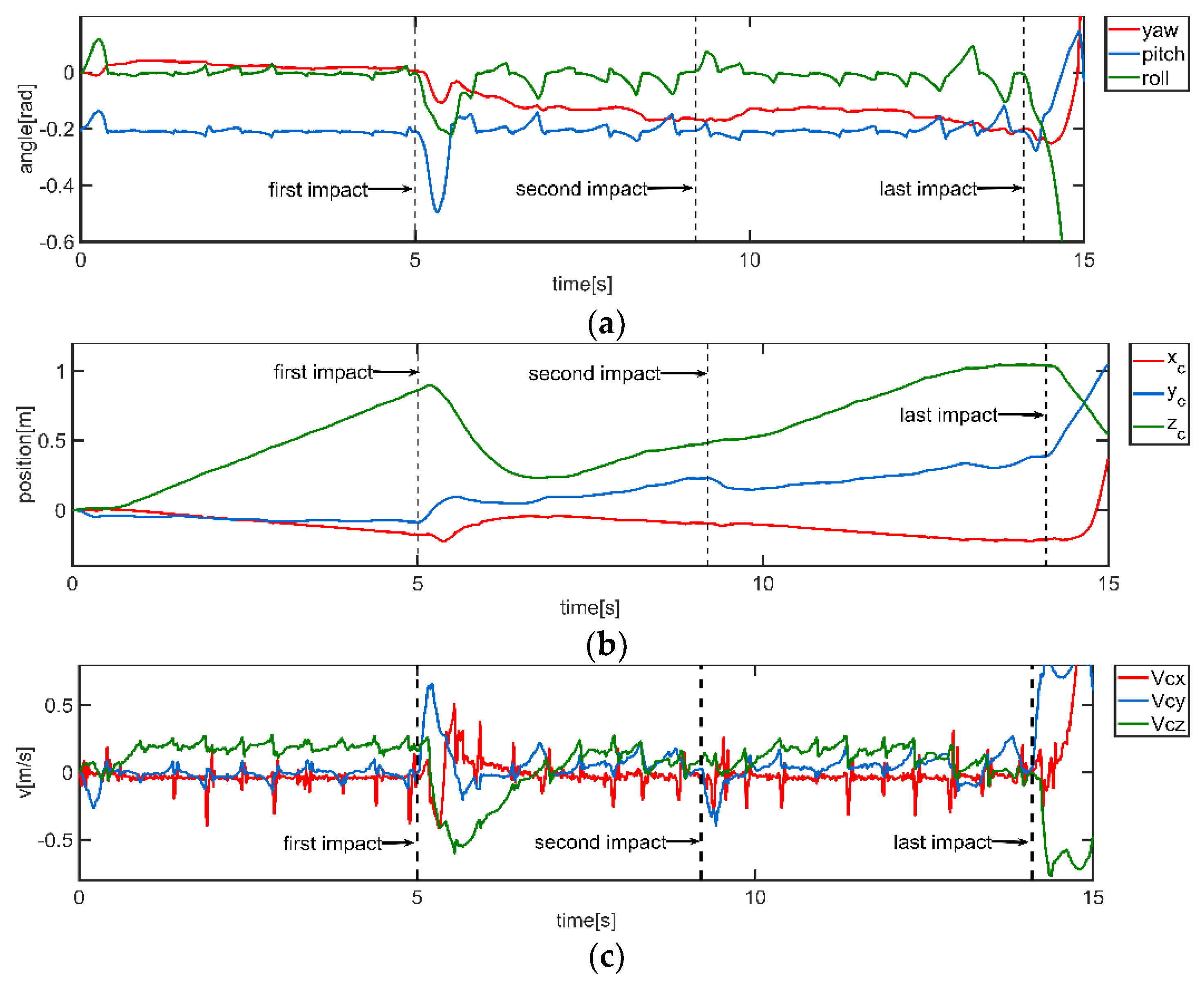
The simulation data from Test 3 were analyzed separately. Here, the three posture angles of the principal-axes coordinate system and the velocities of the body in the
and
directions are shown in
Figure 25 and
Figure 26, respectively.
The impact forces caused large changes in the velocities along the and directions since the current support lines and these forces were not vertical; thus, the posture angles of the body exceeded the angle-fluctuation range of normal stable motion, reducing the stability of the robot. After the first two impacts, the current ground-reaction force prevented the continued increase of undesired speeds in these two directions to a certain extent since ZMP0 was located inside the virtual-support quadrilateral, but did not affect the speed in the direction perpendicular to the support line. This part of speed could only be eliminated when the next set of support feet hit the ground, causing a great impact force at the next set of support feet, such that the stability of the robot was still poor and it had to take several steps for the robot to restore normal stable state. Following the last impact, the speed in the direction, the pitch angle, and the roll angle of the body changed sharply, and the ground-reaction force at the support feet could not prevent the robot from tipping over, and the robot lost its balance.
It can be seen in
Figure 24 that, after the first impact, the distance between
ZMP and the current support line did not exceed the range of the normal stable trotting, and, after the second impact, it was not until 9.8 s that the evaluated stability of Method 1 decreased markedly. Method 2 could show the reduction of the robot’s stability correctly after impacts were applied in this test, but it could not evaluate the stability in time, because LAR was updated when the two feet in the same phase both touch the ground. However, from the curve of Method 3, the stability measurement of the robot decreased very quickly and markedly after the first two impacts and then fluctuated significantly within a few steps after impact. After the last impact, the robot lost its balance. This was consistent with the movement previously analyzed.
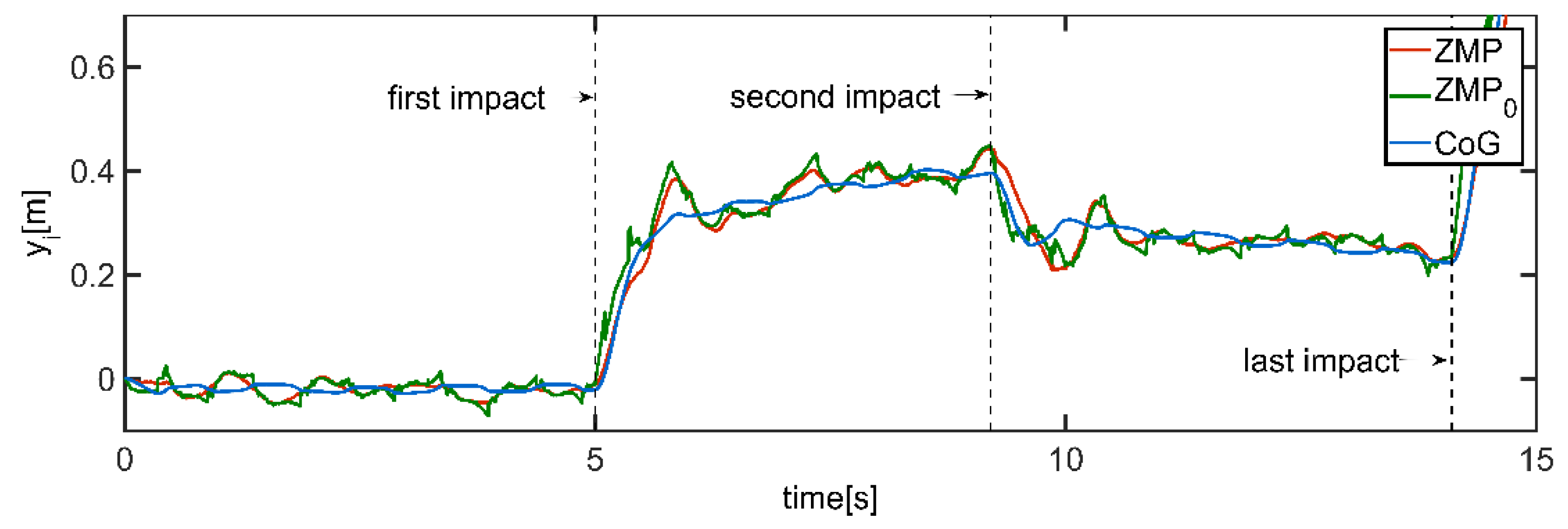
The positions of
ZMP and
ZMP0 were both calculated in this simulation to illustrate that the modified
ZMP with a velocity term can reflect the motion state better than the traditional
ZMP.
Figure 27 shows the curves of
ZMP,
ZMP0, and CoG in the
direction.
After each impact,
of
ZMP0 could show the movement trend faster than that of
ZMP and CoG, and there was not much difference between the peaks (or troughs) of
ZMP and
ZMP0 during the whole movement, meaning that the measurement using
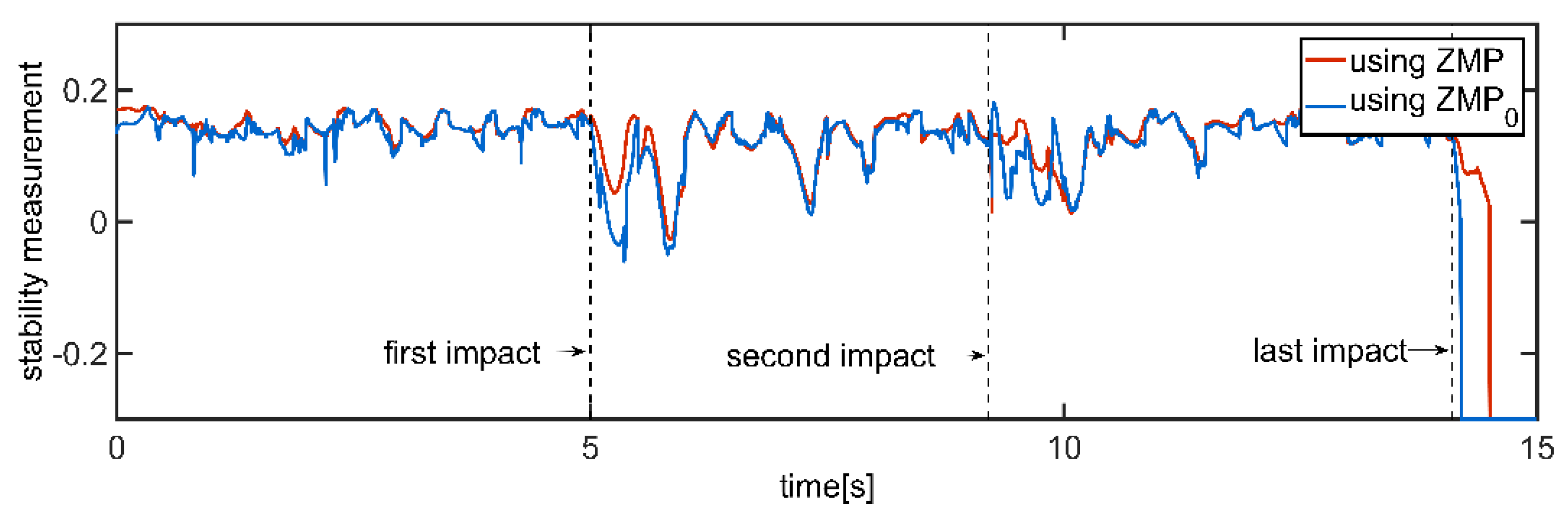
ZMP0 could decrease response time without misjudging the stability state of the robot. As shown in
Figure 28, after the final impact, the stability criterion using
ZMP0 determined that the robot lost its balance at 14.2 s, whereas the criterion using
ZMP showed instability at 14.5 s. The time difference between the two adjacent steps of the trot gait used in this study was 0.5 s. Such a time difference is crucial for the robot to adjust the landing positions of the next support line in time to maintain its balance during robot-motion control.


