Peridynamic Analysis of Rail Squats


Abstract
Featured Application
Abstract
1. Introduction
2. Methods
2.1. State-Based Peridynamic Theory
2.2. Computational Model
2.3. Model of a Rail
2.4. Fatigue Damage Model Parameters
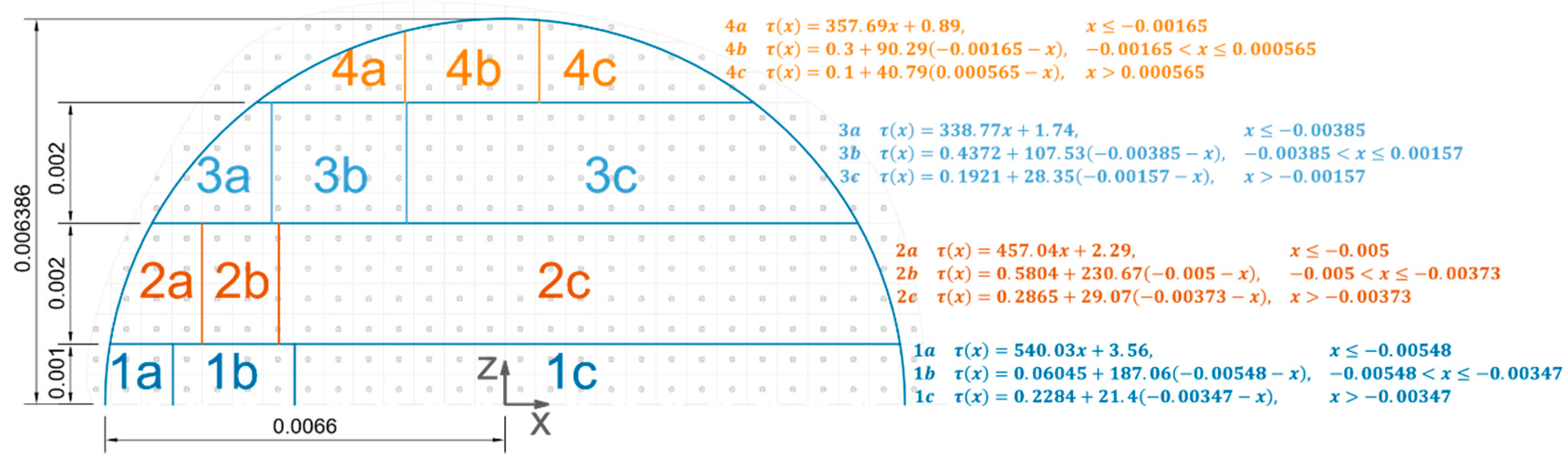
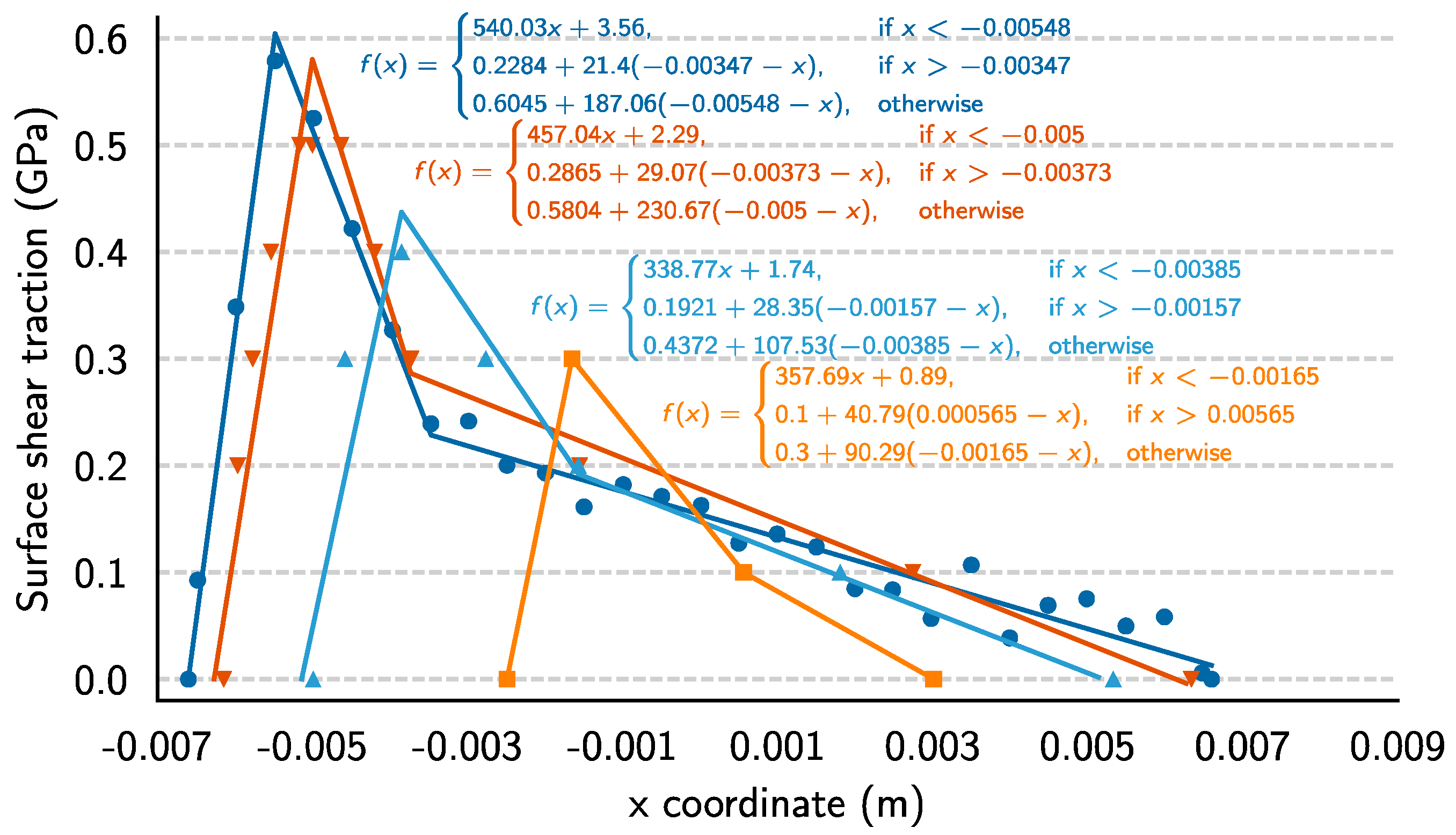
2.5. Boundary Conditions
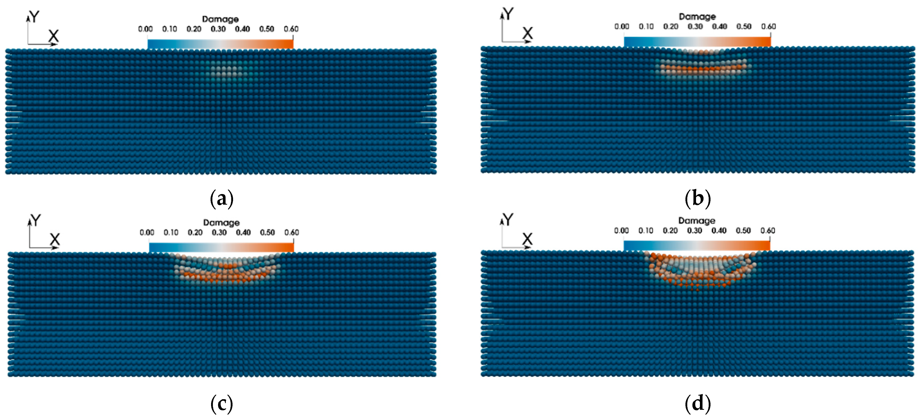
3. Results
4. Discussion and Concluding Remarks
Author Contributions
Funding
Acknowledgments
Conflicts of Interest
References
- Grassie, S.L.; Fletcher, D.I.; Gallardo Hernandez, E.A.; Summers, P. Studs: A squat-type defect in rails. Proc. Inst. Mech. Eng. Part F J. Rail Rapid Transit 2012, 226, 243–256. [Google Scholar] [CrossRef]
- Grassie, S.L. Squats and squat-type defects in rails: The understanding to date. Proc. Inst. Mech. Eng. Part F J. Rail Rapid Transit 2012, 226, 235–242. [Google Scholar] [CrossRef]
- Remennikov, A.M.; Kaewunruen, S. A review of loading conditions for railway track structures due to train and track vertical interaction. Struct. Control Health Monit. 2008, 15, 207–234. [Google Scholar] [CrossRef]
- Kaewunruen, S.; Remennikov, A.M. Progressive failure of prestressed concrete sleepers under multiple high-intensity impact loads. Eng. Struct. 2009, 31, 2460–2473. [Google Scholar] [CrossRef]
- Kaewunruen, S.; Remennikov, A.M. Dynamic properties of railway track and its components: Recent findings and future research direction. Insight Non-Destr. Test. Cond. Monit. 2010, 52, 20–22. [Google Scholar] [CrossRef]
- Carden, E.P. Vibration Based Condition Monitoring: A Review. Struct. Health Monit. 2004, 3, 355–377. [Google Scholar] [CrossRef]
- Kaewunruen, S.; Remennikov, A.M. On the residual energy toughness of prestressed concrete sleepers in railway track structures subjected to repeated impact loads. Electron. J. Struct. Eng. 2013, 13, 41–61. [Google Scholar]
- Seo, J.; Kwon, S.; Jun, H.; Lee, D. Numerical stress analysis and rolling contact fatigue of White Etching Layer on rail steel. Int. J. Fatigue 2011, 33, 203–211. [Google Scholar] [CrossRef]
- Li, Z.; Zhao, X.; Dollevoet, R.; Molodova, M. Differential wear and plastic deformation as causes of squat at track local stiffness change combined with other track short defects. Veh. Syst. Dyn. 2008, 46, 237–246. [Google Scholar] [CrossRef]
- Li, Z.; Zhao, X.; Esveld, C.; Dollevoet, R.; Molodova, M. An investigation into the causes of squats-Correlation analysis and numerical modeling. Wear 2008, 265, 1349–1355. [Google Scholar] [CrossRef]
- Li, Z.; Zhao, X.; Dollevoet, R. An approach to determine a critical size for rolling contact fatigue initiating from rail surface defects. Int. J. Rail Transp. 2017, 5, 16–37. [Google Scholar] [CrossRef]
- Zhao, X.; An, B.; Zhao, X.; Wen, Z.; Jin, X. Local rolling contact fatigue and indentations on high-speed railway wheels: Observations and numerical simulations. Int. J. Fatigue 2017, 103, 5–16. [Google Scholar] [CrossRef]
- Freimanis, A.; Kaewunruen, S.; Ishida, M. Peridynamics Modelling of Rail Surface Defects in Urban Railway and Metro Systems. Proceedings 2018, 2, 1147. [Google Scholar] [CrossRef]
- Kaewunruen, S.; Ishida, M. In Situ Monitoring of Rail Squats in Three Dimensions Using Ultrasonic Technique. Exp. Tech. 2016, 40, 1179–1185. [Google Scholar] [CrossRef]
- Silling, S.A. Reformulation of elasticity theory for discontinuities and long-range forces. J. Mech. Phys. Solids 2000, 48, 175–209. [Google Scholar] [CrossRef]
- Silling, S.A.; Epton, M.; Weckner, O.; Xu, J.; Askari, E. Peridynamic states and constitutive modeling. J. Elast. 2007, 88, 151–184. [Google Scholar] [CrossRef]
- Hu, Y.L.L.; De Carvalho, N.V.V.; Madenci, E. Peridynamic modeling of delamination growth in composite laminates. Compos. Struct. 2015, 132, 610–620. [Google Scholar] [CrossRef]
- Hu, Y.; Madenci, E.; Phan, N. Peridynamics for predicting damage and its growth in composites. Fatigue Fract. Eng. Mater. Struct. 2017, 40, 1214–1226. [Google Scholar] [CrossRef]
- Kilic, B.; Agwai, A.; Madenci, E. Peridynamic theory for progressive damage prediction in center-cracked composite laminates. Compos. Struct. 2009, 90, 141–151. [Google Scholar] [CrossRef]
- Bobaru, F.; Ha, Y.D.; Hu, W. Damage progression from impact in layered glass modeled with peridynamics. Cent. Eur. J. Eng. 2012, 2, 551–561. [Google Scholar] [CrossRef]
- Bobaru, F.; Zhang, G. Why do cracks branch? A peridynamic investigation of dynamic brittle fracture. Int. J. Fract. 2016, 196, 1–40. [Google Scholar] [CrossRef]
- Perré, P.; Almeida, G.; Ayouz, M.; Frank, X. New modelling approaches to predict wood properties from its cellular structure: Image-based representation and meshless methods. Ann. For. Sci. 2015, 73. [Google Scholar] [CrossRef]
- Gerstle, W.; Sau, N.; Sakhavand, N. On Peridynamic Computational Simulation of Concrete Structures; American Concrete Institute, ACI Special Publication: Detroit, MI, USA, 2009; pp. 245–264. ISBN 9781615678280. [Google Scholar]
- Shen, F.; Zhang, Q.; Huang, D. Damage and Failure Process of Concrete Structure under Uniaxial Compression Based on Peridynamics Modeling. Math. Probl. Eng. 2013, 2013, 631074. [Google Scholar] [CrossRef]
- Yaghoobi, A.; Chorzepa, M.G. Meshless modeling framework for fiber reinforced concrete structures. Comput. Struct. 2015, 161, 43–54. [Google Scholar] [CrossRef]
- De Meo, D.; Diyaroglu, C.; Zhu, N.; Oterkus, E.; Amir Siddiq, M. Modelling of stress-corrosion cracking by using peridynamics. Int. J. Hydrogen Energy 2016, 41, 6593–6609. [Google Scholar] [CrossRef]
- Bobaru, F.; Foster, J.T.; Geubelle, P.H.; Silling, S.A. Handbook of Peridynamic Modeling; CRC Press: Boca Raton, FL, USA, 2016; ISBN 9781482230437. [Google Scholar]
- Madenci, E.; Oterkus, E. Peridynamic Theory and Its Applications; Springer: New York, NY, USA, 2014; ISBN 978-1-4614-8464-6. [Google Scholar]
- Silling, S.A.; Lehoucq, R.B. Peridynamic theory of solid mechanics. Advances in Applied Mechanics. Adv. Appl. Mech. 2010, 44, 73–168. [Google Scholar]
- Seleson, P.; Parks, M. On the Role of the Influence Function in the Peridynamic Theory. Int. J. Multiscale Comput. Eng. 2011, 9, 689–706. [Google Scholar] [CrossRef]
- Silling, S.A.; Askari, E. A meshfree method based on the peridynamic model of solid mechanics. Comput. Struct. 2005, 83, 1526–1535. [Google Scholar] [CrossRef]
- Silling, S.; Askari, A. Peridynamic Model for Fatigue Cracks SANDIA REPORT SAND2014-18590; Sandia National Laboratories: Albuquerque, NM, USA, 2014.
- Zhang, G.; Le, Q.; Loghin, A.; Subramaniyan, A.; Bobaru, F. Validation of a peridynamic model for fatigue cracking. Eng. Fract. Mech. 2016, 162, 76–94. [Google Scholar] [CrossRef]
- Jung, J.; Seok, J. Mixed-mode fatigue crack growth analysis using peridynamic approach. Int. J. Fatigue 2017, 103, 591–603. [Google Scholar] [CrossRef]
- Jung, J.; Seok, J. Fatigue crack growth analysis in layered heterogeneous material systems using peridynamic approach. Compos. Struct. 2016, 152, 403–407. [Google Scholar] [CrossRef]
- Oterkus, E.; Guven, I.; Madenci, E. Fatigue failure model with peridynamic theory. In Proceedings of the ITherm 2010: 12th IEEE Intersociety Conference on Thermal and Thermomechanical Phenomena in Electronic Systems, Las Vegas, NV, USA, 2–5 June 2010. [Google Scholar]
- Baber, F.; Guven, I. Solder joint fatigue life prediction using peridynamic approach. Microelectron. Reliab. 2017, 79, 20–31. [Google Scholar] [CrossRef]
- Parks, M.L.; Littlewood, D.J.; Mitchell, J.A.; Silling, S.A. Peridigm Users’ Guide; Digital Library: Piscataway, NJ, USA, 2012. [Google Scholar]
- Littlewood, D.J. Roadmap for Peridynamic Software Implementation; Sandia National Laboratories: Albuquerque, NM, USA, 2015.
- Scutti, J.J.; Pelloux, R.M.; Fuquen-Moleno, R. Fatigue behavior of a rail steel. Fatigue Fract. Eng. Mater. Struct. 1984, 7, 121–135. [Google Scholar] [CrossRef]
- Ahlström, J.; Karlsson, B. Fatigue behaviour of rail steel—A comparison between strain and stress controlled loading. Wear 2005, 258, 1187–1193. [Google Scholar] [CrossRef]
- Schone, D.; Bork, C.-P. Fatigue Investigations of Damaged Railway Rails of UIC 60 PROFILE. In Proceedings of the 18th European Conference on Fracture: Fracture of Materials and Structures from Micro to Macro Scale, Dresden, Germany, 30 August–3 September 2010. [Google Scholar]
- Eisenmann, J.; Leykauf, G. The Effect of Head Checking on the Bending Fatigue Strength of Railway Rails. In Rail Quality and Maintenance for Modern Railway Operation; Springer: Dordrecht, The Netherlands, 1993; pp. 425–433. [Google Scholar]
- Christodoulou, P.I.; Kermanidis, A.T.; Haidemenopoulos, G.N. Fatigue and fracture behavior of pearlitic Grade 900A steel used in railway applications. Theor. Appl. Fract. Mech. 2016, 83, 51–59. [Google Scholar] [CrossRef]
- Deshimaru, T.; Kataoka, H.; Abe, N. Estimation of Service Life of Aged Continuous Welded Rail. Q. Rep. RTRI 2006, 47, 211–215. [Google Scholar] [CrossRef]
- Cannon, D.F.; Pradier, H. Rail rolling contact fatigue Research by the European Rail Research Institute. Wear 1996, 191, 1–13. [Google Scholar] [CrossRef]
- Bobaru, F.; Yang, M.; Alves, L.F.; Silling, S.A.; Askari, E.; Xu, J. Convergence, adaptive refinement, and scaling in 1D peridynamics. Int. J. Numer. Methods Eng. 2009, 77, 852–877. [Google Scholar] [CrossRef]
- Wei, Z.; Li, Z.; Qian, Z.; Chen, R.; Dollevoet, R. 3D FE modelling and validation of frictional contact with partial slip in compression–shift–rolling evolution. Int. J. Rail Transp. 2016, 4, 20–36. [Google Scholar] [CrossRef]
- Freimanis, A.; Kaewunruen, S.; Ishida, M. Peridynamic Modeling of Rail Squats. In Sustainable Solutions for Railways and Transportation Engineering; El-Badawy, S., Valentin, J., Eds.; GeoMEast 2018. Sustainable Civil Infrastructures; Springer: Cham, Switzerland, 2018. [Google Scholar] [CrossRef]
- Ye, L.Y.; Wang, C.; Chang, X.; Zhang, H.Y. Propeller-ice contact modeling with peridynamics. Ocean Eng. 2017, 139, 54–64. [Google Scholar] [CrossRef]
- Tupek, M.R.; Rimoli, J.J.; Radovitzky, R. An approach for incorporating classical continuum damage models in state-based peridynamics. Comput. Methods Appl. Mech. Eng. 2013, 263, 20–26. [Google Scholar] [CrossRef]
- Ferdous, W.; Manalo, A.; Van Erp, G.; Aravinthan, T.; Kaewunruen, S.; Remennikov, A.M. Composite railway sleepers–Recent developments, challenges and future prospects. Comp. Struct. 2015, 134, 158–168. [Google Scholar] [CrossRef]
- Kaewunruen, S.; Chiengson, C. Railway track inspection and maintenance priorities due to dynamiccoupling effects of dipped rails and differential track settlements. Eng. Fail. Anal. 2018, 93, 157–171. [Google Scholar] [CrossRef]
- Kaewunruen, S.; Sussman, J.M.; Matsumoto, A. Grand challenges in transportation and transit systems. Front. Built Environ. 2016, 2, 4. [Google Scholar] [CrossRef]


| Parameter | Volume, m3 | % Difference |
|---|---|---|
| Cubic | 1.25000 × 10⁻¹⁰ | 0.00% |
| Min | 1.18960 × 10⁻¹⁰ | −4.83% |
| Max | 1.29750 × 10⁻¹⁰ | 3.80% |
| Average | 1.26464 × 10⁻¹⁰ | 1.17% |
| Value | X | Y | ||||
|---|---|---|---|---|---|---|
| FE, m | PD, m | Difference | FE, m | PD, m | Difference | |
| Max | 2.03 × 10⁻⁵ | 1.90 × 10⁻⁵ | −6.95% | 2.35 × 10⁻⁶ | 2.55 × 10⁻⁶ | 7.92% |
| Min | −6.59 × 10⁻⁷ | −8.30 × 10⁻⁷ | 20.61% | −4.69 × 10⁻⁵ | −5.07 × 10⁻⁵ | 7.48% |
| Phase I | Phase II | |
|---|---|---|
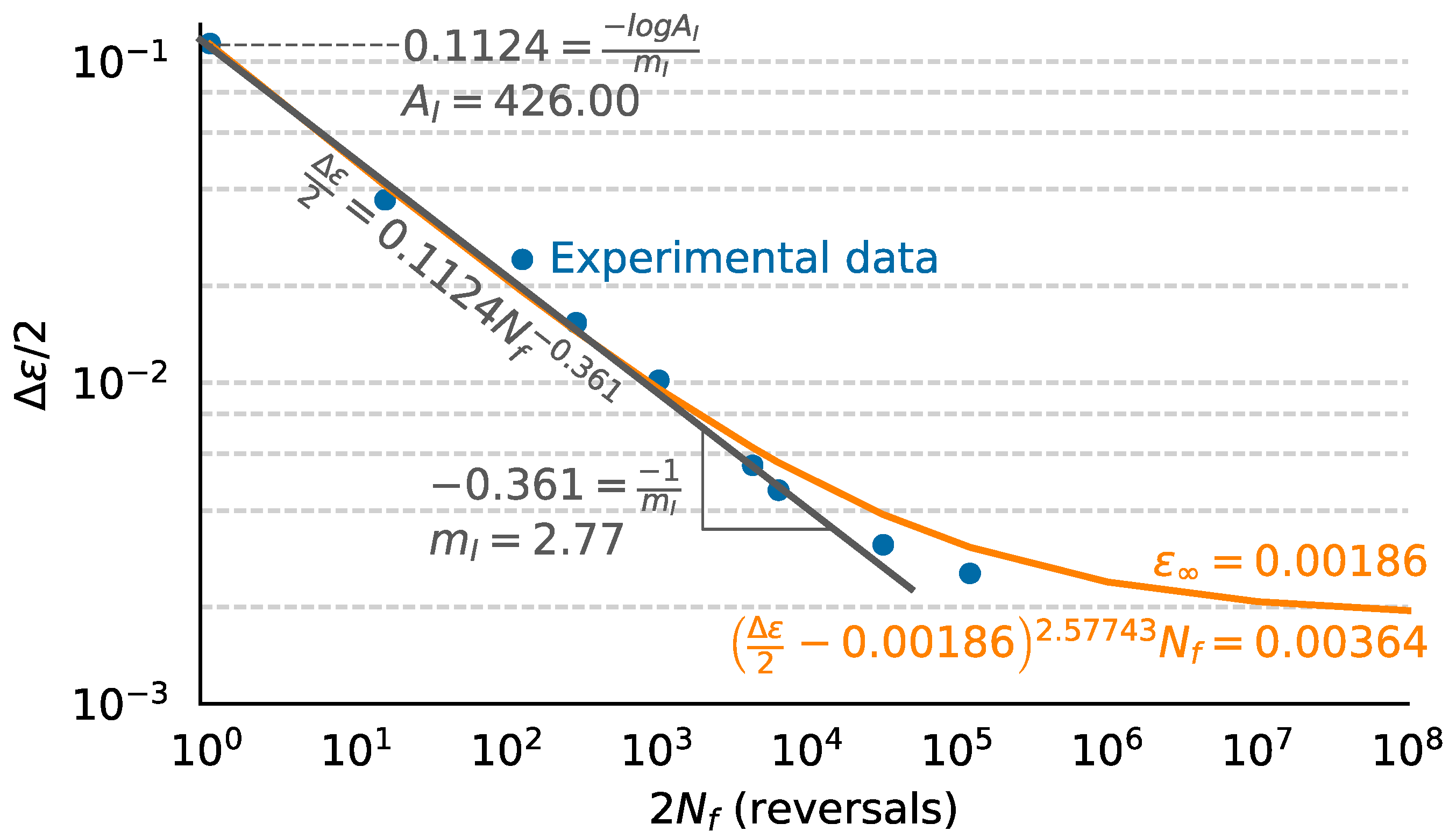
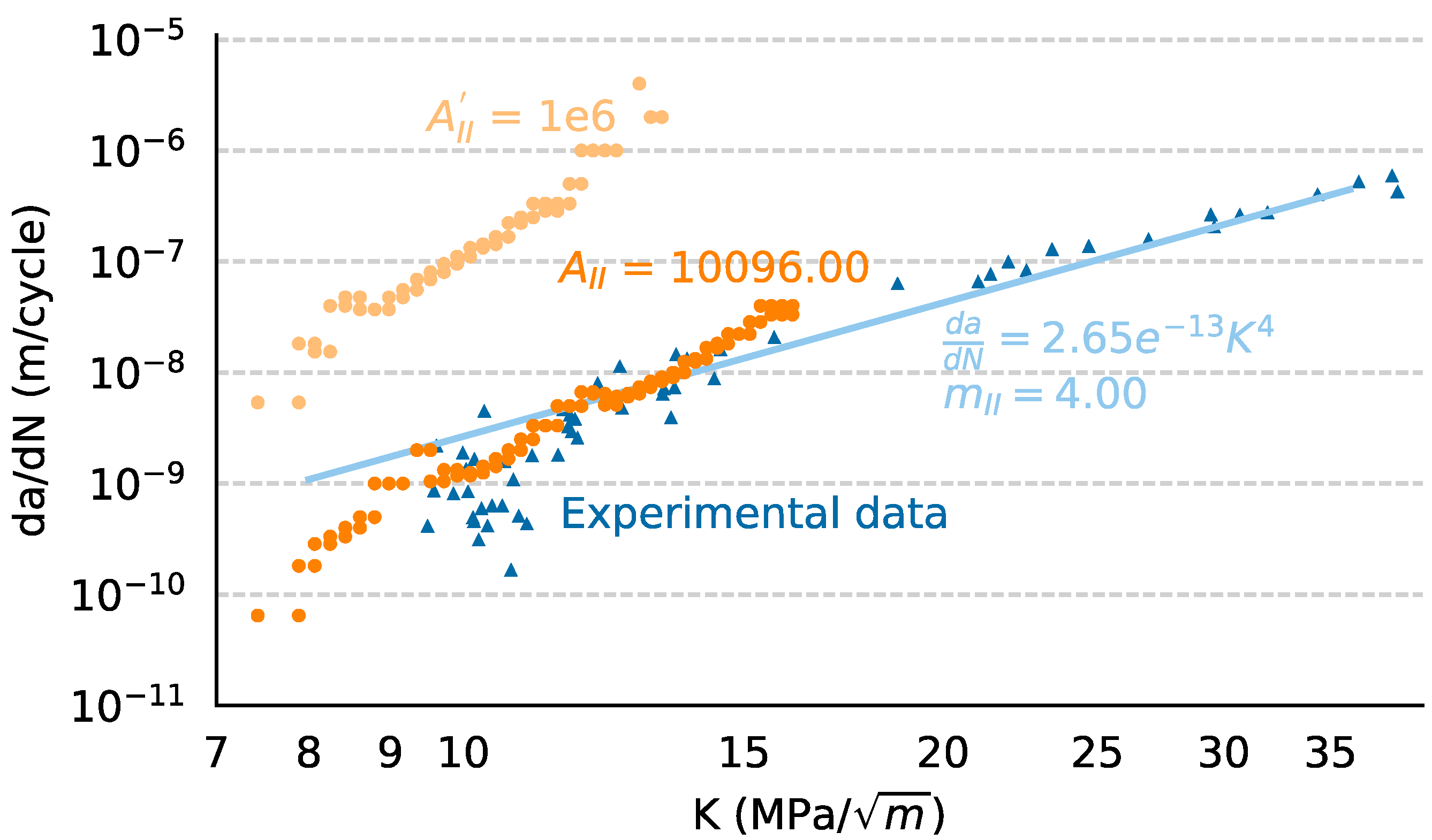
| A | 426.00 | 25,237.48 |
| m | 2.77 | 4.00 |
| ε∞ | 0.00186 | -- |
© 2018 by the authors. Licensee MDPI, Basel, Switzerland. This article is an open access article distributed under the terms and conditions of the Creative Commons Attribution (CC BY) license (http://creativecommons.org/licenses/by/4.0/).
Share and Cite
Freimanis, A.; Kaewunruen, S. Peridynamic Analysis of Rail Squats. Appl. Sci. 2018, 8, 2299. https://doi.org/10.3390/app8112299
Freimanis A, Kaewunruen S. Peridynamic Analysis of Rail Squats. Applied Sciences. 2018; 8(11):2299. https://doi.org/10.3390/app8112299
Chicago/Turabian StyleFreimanis, Andris, and Sakdirat Kaewunruen. 2018. "Peridynamic Analysis of Rail Squats" Applied Sciences 8, no. 11: 2299. https://doi.org/10.3390/app8112299
APA StyleFreimanis, A., & Kaewunruen, S. (2018). Peridynamic Analysis of Rail Squats. Applied Sciences, 8(11), 2299. https://doi.org/10.3390/app8112299