1. Introduction
Good control of the production parameters is required for producing precision parts. Which production parameters to choose and which tolerances they should have can be best determined when the process is well understood. When casting thermoset polymers an important and fundamental aspect is the understanding of the curing process [
1,
2,
3,
4,
5]. A complete cure is required to obtain good mechanical properties. Curing also causes shrinkage that can influence the surface quality of the component. Depending on the geometry of the part, thermal and curing shrinkage can also create internal stresses that can weaken the part or lead to cracking [
6,
7,
8,
9,
10,
11,
12]. Further, the heat generated during the cure in an exothermic reaction needs to be controlled. When the heat cannot be removed from the inside of the component, temperature increases substantially and the properties of the polymer may degrade, even leading to a fire in the worst case. The control of the heat development is especially important for big components having a large volume to surface ratio, since, due to the low heat conductivity of most polymers, the heat cannot be removed easily [
13,
14].
This paper describes how heat development during the cure of a polymer can be predicted and how the necessary material properties are obtained. In principle all required steps are well known, but a practical approach that an industrial user can utilize is lacking. The main practical challenge is that the detailed composition of the polymer is typically not known in engineering applications [
1]. The producer of the polymer does not give that information to the manufacturer for commercial reasons. Without knowing the exact composition of the polymer the manufacturer cannot use information directly from the literature. Even if the manufacturer had the full knowledge of all details of the polymer, the specific properties required for cure modeling would likely not be readily available. This paper provides an approach that gives the manufacturer of components sufficient information with relatively little test effort to predict the heat development during curing.
This paper describes first briefly the basic theory behind curing kinetics and the challenges for the general user. It shows then how the required properties can be measured using relatively simple methods. A key practical aspect is that the measured results should allow sufficiently accurate prediction of the curing behavior. However, the results may not be good enough to characterize the curing kinetics in all detail, as it is not needed for the manufacturer. This simplification makes it possible to give the manufacturer a simple procedure to get the data needed for production modelling. Emphasis will be put on some critical details that need to be considered in the data analysis. Finally it will be shown how the measurement results can be used in a slightly modified commercial finite element program to predict curing behavior. The subroutines needed to modify the program will be explained.
The procedures will be explained for an example of casting a large block of a filled two-component thermoset polyurethane. The curing reaction is exothermic. The polyurethane is used for casting large components (rings of about 1 m diameter and 30 cm thickness and width) with metallic inserts. This paper presents the simplified case of casting a block of mm3.
2. Cure Modeling and Heat Generation
The conversion
(or degree of cure) is the amount of bonds formed in a certain amount of polymer. The rate
at which bonds are formed with time
t during a chemical reaction is typically described with a general rate equation [
15,
16]:
The so called kinetic function
will be discussed below,
T is the absolute temperature and
k the rate coefficient. The latter relates to the temperature according to the empirical Arrhenius equation [
17,
18] which appears in the right hand side of Equation (
1) instead of
k. In the Arrhenius equation
R is the universal gas constant,
E the activation energy and
A the pre-exponential factor. The exact physical meaning of
A is out of scope of this article, but in general it determines how often molecules collide with each other. Note that
is given as a normalized quantity ranging from 0 (no bonds) to 1 (fully cured). The rate of reaction
should change with the number of bonds that have already formed. This change can be described by the kinetic function
. Intuitively one could think that the reactants can find possible sites for bonding easily at the beginning of the curing process. Once many bonds have formed the reaction rate slows down due to a limited number of available sites. Depending on the chemistry involved many scenarios are possible. Much work has been done to determine the functions
for various chemical reactions and we refer to
Table 1 in
Section 3.2 for some of them. While traditionally it was assumed that
k is only dependent on the temperature, a growing body of works shows that both
E and
A can be dependent on
(see for example [
19,
20,
21,
22,
23,
24,
25,
26,
27,
28,
29]).
The formation of polymer bonds is an exothermic reaction. During each bond formation a certain amount of heat
Q is released. If, in a given amount of polymer, all bonds are formed, the total heat
(usually normalized to one gram) is released (cf.
Figure 1b and text). The heat set free during a chemical reaction can be measured with a standard experimental procedure as described in more detail below. The rate at which bonds are forming is related to the released heat. This relationship is expressed in the equation:
The quantities
and
are of primary interest for the practical user. If the former can be calculated as the integral of Equation (
1), the latter can easily be obtained as the integral of Equation (
2). This has an important implication. It is sufficient to model the integral of the reaction equations accurately. This means typically that certain inaccuracies in the reaction equations can be acceptable, because they play a minor role in the integrated quantities. This will be discussed in more detail throughout the paper.
The equations also show that the main parameters to be obtained are: E, A and ; which is often called the “kinetic triplet”. The following will describe how these parameters can be obtained at sufficient accuracy.
2.1. Heat Flow Measurements by Differential Scanning Calorimetry
Several techniques exist to investigate the curing of polymers. Raman or infrared spectroscopy [
30,
31,
32,
33] allows investigation of the reaction mechanisms. However, these techniques can not analyze the often very weak signals at high conversion. Measuring the dielectric properties (utilizing dielectric analysis –DEA) [
33] or the change of the internal structure (using ultrasound) [
34,
35] of the polymer are other methods to characterize the curing process. However, these provide the user not with thermal data.
Judging from the literature curing characteristics are most often measured with Differential Scanning Calorimetry (DSC). DSC is a versatile, well known and long established material characterization technique [
15,
16].
In this case DSC is used to determine the exothermic heat created by the curing process of the thermoset polymer, as it turns from a viscous liquid into a solid by cross-linking [
36,
37,
38,
39,
40,
41,
42,
43,
44,
45,
46,
47,
48,
49,
50]. It is assumed that no other phase transitions occur absorbing or developing heat. Knowing the progression of the curing reaction and the related energy allows calculation of the heat release in a given volume in finite element simulations.
In the following we will provide a brief overview of the DSC method, which should enable the reader to understand the results of this paper. More details can be found in [
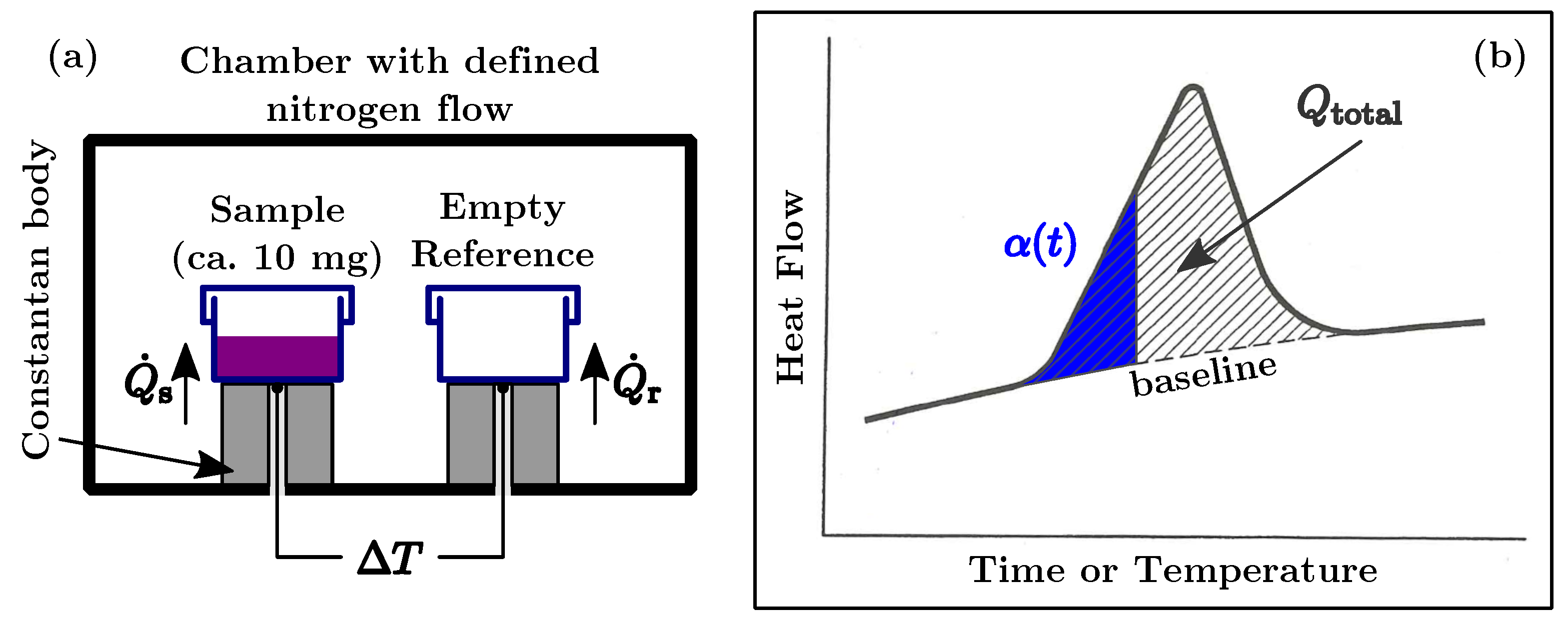
15]. The DSC related equations shown here are also taken from this reference and the same symbols are used. A DSC apparatus is basically a chamber with a defined gas flow (often nitrogen) that contains two similar pans on a constantan body. A sketch of such a setup can be seen in the
Figure 1a.
One pan contains the sample, the other one is empty and acts as reference. The temperature difference between both pans is measured while the temperature is ramped up. In isothermal experiments the heating rate is constant, while a temperature ramp is applied to both pans in dynamic experiments. Temperature differences occur either when the temperature of the constantan body is raised and the thermal inertia of the sample takes up more heat (this happens for any material) or when phase changes occur. Examples of the latter would be melting or transitioning from the glassy to the rubbery state. However, none of these are relevant for the data and results presented here. Another cause for a temperature difference are chemical reactions taking place in the sample pan (as in the case of a curing polymer). Since both pans are similar (in material and mass) and are placed on the same constantan body, any difference in temperature between the sample and the reference pan is solely due to the sample itself. Leaving all particulars aside, the heat flow
is simply proportional to the temperature difference between the containers:
and
denote the sample and reference heat flow respectively. A DSC instrument measures the temperature difference very accurately, see e.g., [
15]. Of interest here is the dependency of the released heat on time or (change of) temperature since it embodies the information needed to simulate the heat released during cure.
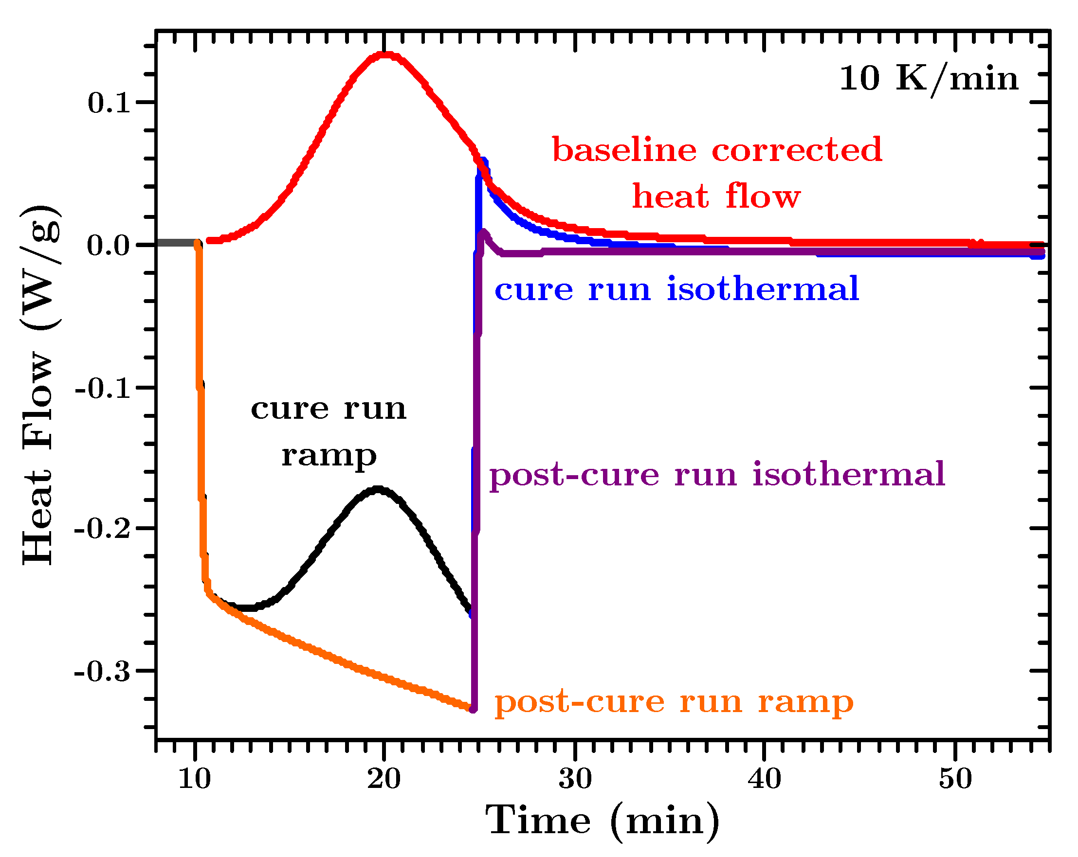
A DSC curve shows the heat flow over time (or temperature in dynamic experiments). A curing reaction exhibits an exothermal heat flow peak over a baseline. A simplified sketch is shown in
Figure 1b. The baseline is the heat flow during steady state conditions [
15]. The peak above the baseline is the total heat of curing
. By integrating Equation (
2) the time (or later temperature) dependent degree of cure
can easily be calculated directly from the DSC measurements.
It is necessary to determine the baseline of the DSC curve to be able to calculate
and
. In reality the baseline is a sigmoid and several, more or less complicated, techniques exist to calculate it. However, very often simply a straight line is used between the start- and end-point of the exothermic peak [
15,
42,
51,
52,
53,
54,
55,
56]. If the change in heat capacity during the exothermic peak is insignificant a straight line is justified [
15,
55].
The procedure to obtain the baseline will also influence
. However, choosing a straight line gives just a small error of
relative to the scatter of
between samples [
56].
Appendix C gives a detailed example on how to perform the baseline correction of the heat flow data for isothermal and dynamic measurements.
Dynamic DSC experiments are typically run at a constant rate of increasing temperature. The rate may be changed from experiment to experiment. Since the time to cure depends on the characteristics of chemical reaction, dynamic DSC experiments under different conditions allows obtaining the kinetic triplet parameters from Equation (
1).
The standard way to obtain the kinetic triplet is regular fitting of DSC data with a given kinetic function [
4,
57]. Here, and in the following, the term “regular fitting” shall describe that the parameters of a given function are optimized until said function describes the data in question. If for example it is assumed that
in Equation (
1) than the function that needs to be optimized is
. In this example the values for
A,
E and
n are initially guessed and said function will be calculated. Then the values for these three parameters will be changed and the function calculated again until the deviation between the function with optimized parameters and the data is below a given threshold.
If the chemical composition of the constituents and the chemical pathways are known, it is possible to arrive at the kinetic function by studying the rate equations of the underlying chemical reactions [
58,
59]. However, this research was done for the practical case where no detailed information of the involved chemicals was available (cf.
Section 5.2).
Two other methods shall be mentioned which enable a user to simulate the curing process of a polymer: Molecular dynamic calculations [
60] and thermodynamic frameworks [
61]. However, these are rather involved, require extensive mathematical frameworks, can not easily be used in standard finite element software and are not suitable for the simulation of large structures with today’s computational technology.
3. Utilizing the Isoconversional Method and the Compensation Effect to Calculate the Actual Kinetic Model
If the polymer under investigation does not behave according to an idealized reaction model or if this model
is not known it may not be possible to acquire the correct kinetic triplet by regular fitting of the DSC data as described above. In such cases the isoconversional method allows obtaining the activation energy in dependency of the conversion without having to know anything about the kinetic model. Below we present just the final results of the theory extensively laid out in the works of Vyazovkin and others [
19,
20,
21,
22,
23,
25,
27,
29]. The theory assumes that the Arrhenius prefactor
A and the activation energy
E in Equation (
1) are also dependent on the degree of cure, thus becoming
and
. A more detailed derivation and justification for these equations can be found in
Appendix A.
A certain degree of theoretical background needs to be given to make the used methods understandable at all. However, at the end of each subsection a short summary of the quintessence is given. A potential user needs to obtain just dynamic DSC data and needs to code simple programs to calculate the kinetic triplet or use software that can be found online (either commercial or in common software repositories).
3.1. The Isoconversional Method to Determine the Activation Energy
Considering several DSC experiments with constant, but different temperature ramps with heating rates
. Then the essence of the isoconversional method is the following equation:
in which
stands for the value of the double sum on the right side. The reader may observe that this equation does neither contain the kinetic model nor the pre-factor. The indices
i and
j denote different experiments,
n is the total number of experiments and
J is an abbreviation for the following integral:
J is basically an integral over the Arrhenius equation. The upper limit is the temperature when the polymer reached the degree of cure of interest and the lower limit is the temperature when the material reached a lower conversion.
For a given conversion
, the limits of the integral in Equation (
5) follow directly from the heat flow data. Then the integral(s) themself are calculated by first choosing an arbitrary value for
(the initial guess) and computing the double sum. This yields a value for
. Next another value for
is chosen while the integral limits stay the same and the ingrals and double sum are calculated with this new value for
. This yields another value for
. This algorithm is then repeated until an activation energy is found for which
is minimal.
DSC measurements with arbitrary temperature programs can be analyzed by equalling the heating rate(s)
in Equation (
4) to one (no matter what the actual heating rate was) and in Equation (
5) the integral is performed over time instead of temperature. A more detailed derivation and justification for these equations can be found in
Appendix A.
is an integral which is evaluated over all the available data for Equation (
4). Thus, the influence of any (random) experimental errors will be small since random fluctuations play a minor role in the integrated values.
A summary of the above is the following: First the baseline corrected heat flow data of all experiments is used to obtain the limits of the integral in Equation (
5) and the same is calculated. Afterwards the double sum in Equation (
4) is minimized as described above to determine the activation energy for each degree of cure between zero and 100% in steps determined by the user.
3.2. The Compensation Effect to Determine the Pre-Factor
Determining the pre-factor
A in the Arrhenius equation is independent of the isoconversional method decribed above. If Equation (
1) is rearranged the following relationship is obtained:
Here the index
k denotes different kinetic models as for example given in
Table 1.
The time dependency of the conversion follows directly from the DSC data (cf. Equation (
2)) and thus is known. For each
, the inverse of the different kinetic functions can simply be calculated. Hence, the left hand side of Equation (
6) is known for each time
t. Since constant heating rates are assumed, time and temperature correlate linearly with each other. The left hand side of Equation (
6) over the inverse temperature needs then to be linearly fitted for each model
k. This will yield different sets of
and
. It has to be mentioned that here, and only here, the pre-factor and activation energy are not considered to be dependent on the conversion.
After sets of
and
are determined for different models
k (e.g., all the models in
Table 1) it was shown [
62,
63,
64,
65,
66,
67] that these lie all on a line and the following linear relationship holds true:
This is the so called compensation effect with the compensation parameters a and b. The interested reader is refered to the cited sources for a justification of these equations.
Once the compensation parameters are known the conversion dependent pre-factor can easily be determined by:
A summary of the above is the following: The baseline corrected heat flow data of all dynamic experiments is taken to calculate the left hand side of Equation (
6) for all models given in
Table 1. Then these values are fitted over the inverse temperature for
to obtain the sets of
and
. The interval of
was chosen as proposed by Alzina et al. [
24]. However, smaller or larger intervals have no significant influence on the values of the compensation parameters.
Finally, as described above, a linear fit over all these sets yields a and b.
3.3. Calculating the Actual Kinetic Model
After the activation energy
and the pre-factor
have been determined for sufficiently small increments of the degree of cure, Equation (
1) can be re-arranged to:
Since
is known directly from the heat flow data (cf. Equation (
2)), Equation (
9) can be used to calculate the actual kinetic model which governed the curing reaction. The calculated kinetic function
can than be plotted vs.
and can be parametrized as the user wishes. It can also be compared with each of the idealized kinetic models given in
Table 1 to chose an appropriate model. However, it should be noted that the approach shown here needs only
and a match with a known model is not needed.
4. Heat Capacity and Heat Conductivity
Two additional quantities are needed for the cure simulations of components. The first is the heat capacity of the polymer. The dependence of the heat capacity on the degree of curing and the temperature needs to be established. So called temperature modulated DSC was utilized to determine this property. The specifics of this method are out of scope of this article. Thus we refer the interested reader exemplary to the works of e.g., Höhne et al. [
15] or Schawe and others [
39,
41,
43,
44,
47,
48,
68,
69,
70,
71,
72] for information about this technique.
Finally, the heat conductivity of the material is needed for the cure simulations. This property can be obtained according to standard methods, such as described in ISO 8301 [
73].
5. Experimental Methods
5.1. General DSC Setup and Procedures
In principle a user of this method needs to perform just a number of dynamic DSC experiments with different heating rates. The above presented methods take this data as input and yield , and . We have performed both dynamic and isothermal DSC experiments. The results obtained by these two different datasets differ little from each other. However, the compensation effect works ony with data that exhibits a temperature ramp. Thus, with two minor exceptions, the input parameters used to perform the simulations were obtained with dynamic DSC data. The exceptions will be discussed in the appropriate sections.
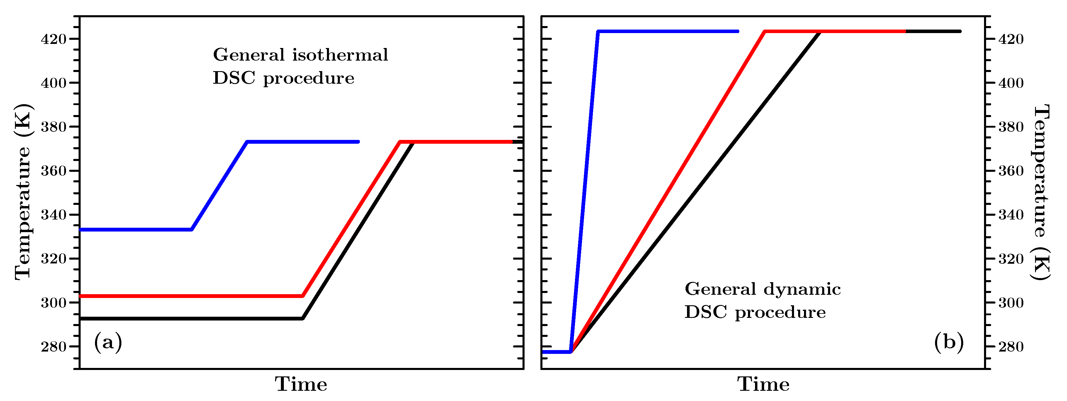
A Discovery DSC 250 from TA Instruments with a TRIOS software package and TZero Pans with TZero hermetic lids were used to acquire the necessary DSC data. The mass of the samples was ca. 10 mg. Seven isothermal and ten dynamic experiments were performed. In all experiments one and the same reference pan was used. Before the experiment started the temperature of the DSC was set to the desired value and the sample pan was carefully placed onto the constantan body. On average 30 s (
s) passed between opening the chamber to place the sample and starting the collection of the data. In isothermal experiments the sample was held for a certain amount of time at a given temperature. In dynamic experiments the samples were heated from 292 K to 423 K with different heating rates and then held at 423 K for 30 min to allow them to reach 100% conversion. A sketch of these two general principles can be found in
Figure 2 and important experimental parameters can be found in
Table 2. In
Appendix B the details how the isothermal and dynamic experiments were performed can be found.
Each experiment was repeated with the fully cured sample to establish the baseline. The reason for this was that for the dynamic experiments no reaction endpoint could be determined from the initial experiment(s) because the sample(s) did not reach 100% conversion during the temperature ramp. An example is shown in
Appendix C. These second experiments exhibited straight heat flow lines. The actual heat flow during the curing of the sample was then determined by subtracting the second run from the first. This can be justified since heat capacity measurements suggest that the material properties are governed by the unknown filler material (cf.
Section 7.2) which is not affected by the chemical reaction or the changing properties of the curing polymer. This simple method is also within the scope of this article to provide a practical approach for engineers to gather data.
All the DSC data was exported to ASCII-files to allow analysis outside the proprietary DSC program.
These experiments provided the input data, which was used to obtain the limits of the integral in Equation (
5) which then were used in Equation (
4) to determine the conversion dependent activation energies. Only the data from the dynamic experiments was utilized to obtain the compensation parameters according to Equation (
6). Afterwards, from both datasets again, the actual kinetic function was calculated using Equation (
9).
Lastly one temperature modulated experiment was performed to investigate the heat capacity properties of the material. The amplitude of the temperature modulation was 1 K over a period of 60 s. A sample of 14.063 mg was first held for 4000 min at 293 K. Thus the dependency of the heat capacity from the degree of cure could be established. Subsequently the temperature was increased with 2 K/min to 423 K to investigate the temperature dependency of the heat capacity of the same (now fully cured) sample.
5.2. Material Preparation
The project partners from whom we got the resin and the hardener could not provide any details about the material except that it was a polyurethane with fillers. It was supposed to exhibit low cure shrinkage and supposedly no chemicals were added to enhance the curing rate. The resin and the fully cured material were pitch black. Resin and hardener were mixed according to manufacturers recommendations.
For the DSC experiments the masses of resin and hardener were controlled within 0.01 g accuracy. Resin and hardener were mixed at room temperature thoroughly for one minute (time accuracy was approximately 5 s). Afterwards the amounts stated in
Table 2 were weighed into the DSC pans within 0.001 mg accuracy. Eight to nine minutes passed between the start of the mixing and placing the samples in the DSC.
For the verification experiment, the mixing was performed by the project partners. The total mass was 4300 g. The resin was pre-heated to 303 K and mixing took place under vacuum in a plastic bucket with a diameter of 185 mm. The mixing time was approximately 8 min and 30 s. Due to technical issues the mixture sat still in the bucket for an unknown amount of time (less than 15 min) before 3790 g were poured into the mold that contained the temperature sensors. The whole experiment took place in an oven that was set to 303 K.
A part of the fully cured material was sent to Norner AS, an external polymer research institution, to measure the thermal conductivity
according to ISO 8301 [
73]. It was determined that
exhibits a linear temperature dependency:
5.3. Setup of the Large Cast Control Experiment
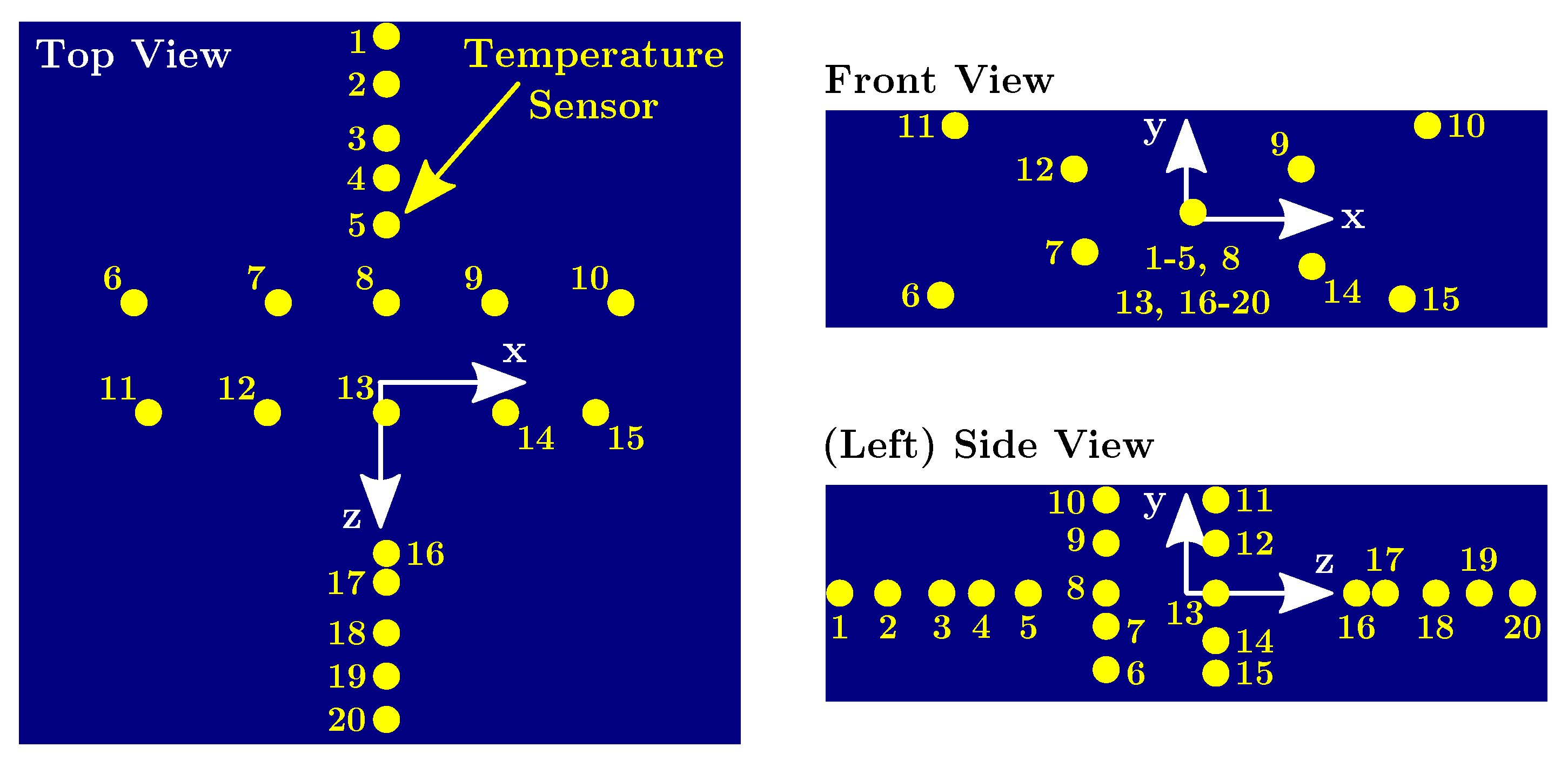
A fairly large rectangular brick was molded to emulate a large-scale commercial cast. To hold an amount of the material that would sufficiently emulate a large scale cast, a mold of stainless steel was constructed. The thickness of the walls was 2 mm. The cavity of the mold had an area of mm2 and a wall height of approximately 11 cm. The mold was filled with material to a height of ca. 6 cm.
The temperature development during the progress of the curing reaction was measured by embedding twenty temperature probes into the material. The sensors were radial glass NTC thermistors, encapsulated in glass with 10 k
resistance at 298 K and a temperature range from 233 K to 523 K. In
Figure 3 the position of the sensors with respect to the point of origin can be seen.
The interval between two subsequent temperature measurements was either 15 min or 3 min, depending on whether the temperature in the middle of the block was below or above 313 K.
6. Finite Element Simulations
A finite element analysis was set up to simulate the curing behavior and to predict the temperature developments of the cast block during curing. The program for finite element simulations was Abaqus 6.14-1 from Dassault Systèmes Simulia Corp. All units of the used variables were stated in SI units. A mesh size of 0.005 was used for the simulations.
For the material properties the temperature dependent thermal conductivity (see
Section 5.2), the specific heat (see
Section 7.2) and the density at room temperature were used.
No mechanical boundary conditions were applied since a heat transfer problem was simulated. An appropriate initial temperature and degree of cure value was applied to all nodes of the mesh (see detailed description below). To simulate convective heat transfer in air on the surface of the body, a surface film condition interaction was implemented in the model. The sink temperature and film coefficient were chosen appropriately, dependent on the simulated conditions (see below).
The simulation of the generation of heat due to curing is done with the HETVAL user subroutine. The routine was used in connection with the conversion in each nodal point as solution dependent variable. To initialize the solution dependent variable the SDVINI user subroutine was utilized which is called once at the start of the simulation. The HETVAL user subroutine reads the temperature and degree of cure in each nodal point. Then it calculates the progress of
during the last time step according to Equation (
1). The heat generated per cubic meter and time for the given step is then calculated according to Equation (
2). The FLUX(1) variable of the HETVAL subroutine is set to this value. Abaqus is then able to calculate the distribution of the heat without further input.
Since the experiment consisted of two steps (mixing in bucket and the actual experiment in the mold) these two needed to be simulated. First the mixing in the bucket with the buckets geometry and 29,757 elements was modeled to determine the initial degree of cure for the simulations of the actual experiment. For this simulation the initial node temperature was set to 303 K, since the resin was pre-heated, and the surrounding temperature was 296 K. The (surface) film coefficient was set to 10 W/m per K, due to the fact that the heat transfer coefficient for convection in air with a low velocity is ca. 10 W/m per K [
74]. The initial conversion was set to zero. The core temperature of the bucket-simulation was the control parameter to determine the initial degree of cure to be used in the block-simulation. When the core reached a temperature of 314 K (the very first temperature measurement), the conversion of said bucket-core was used as initial value for
in the simulations of the block. The mixing process itself was not modeled.
Secondly the actual experiment was simulated with a block of
and 19,200 elements. The initial temperatures at the nodes were set to 314 K (the first measured temperature value) and the initial degree of cure was set to the value determined in the bucket-simulation. The surrounding temperature was set to 303 K but for the film coefficient a value of 20 W/m per K was used. The latter because the heat flux is proportional to the surface area [
74] and the walls of the steel mold in the control experiment were higher than the poured material, thus acting as cooling fins. This additional surface area amounted to approximately a factor of two. Since the mold is not modeled, this area dependency of the heat flux is put into the film coefficient.
7. Results
At this point we want to point out again that all of the results in connection with the isoconversional method can be calculated with data from just dynamic experiments. However, since the material investigated was supposed to be slow curing, we expected the simulations to be rather isothermal-like from one time step to the other than with fast rising temperatures as in dynamic DSC experiments. Hence, we performed also isothermal experiments as a control measure on how good the determined parameters are. Since the isothermal data was available to us we performed also all calculations with it and the results did not change significantly. This will be shown for the activation energy and the actual kinetic model. However, two minor differences compared to the dynamic results were the mean total heat value and the activation energy for low conversions. Again, since the data was available for us, we did not reject these two minor differences, since this allowed us to easily get slightly better simulations. This will be discussed in the appropriate sections.
7.1. Isothermal and Dynamic Experiments
All heat flow data is baseline corrected as described in
Section 5.1 and
Appendix C to obtain the heat flow related to the curing of the polymer.
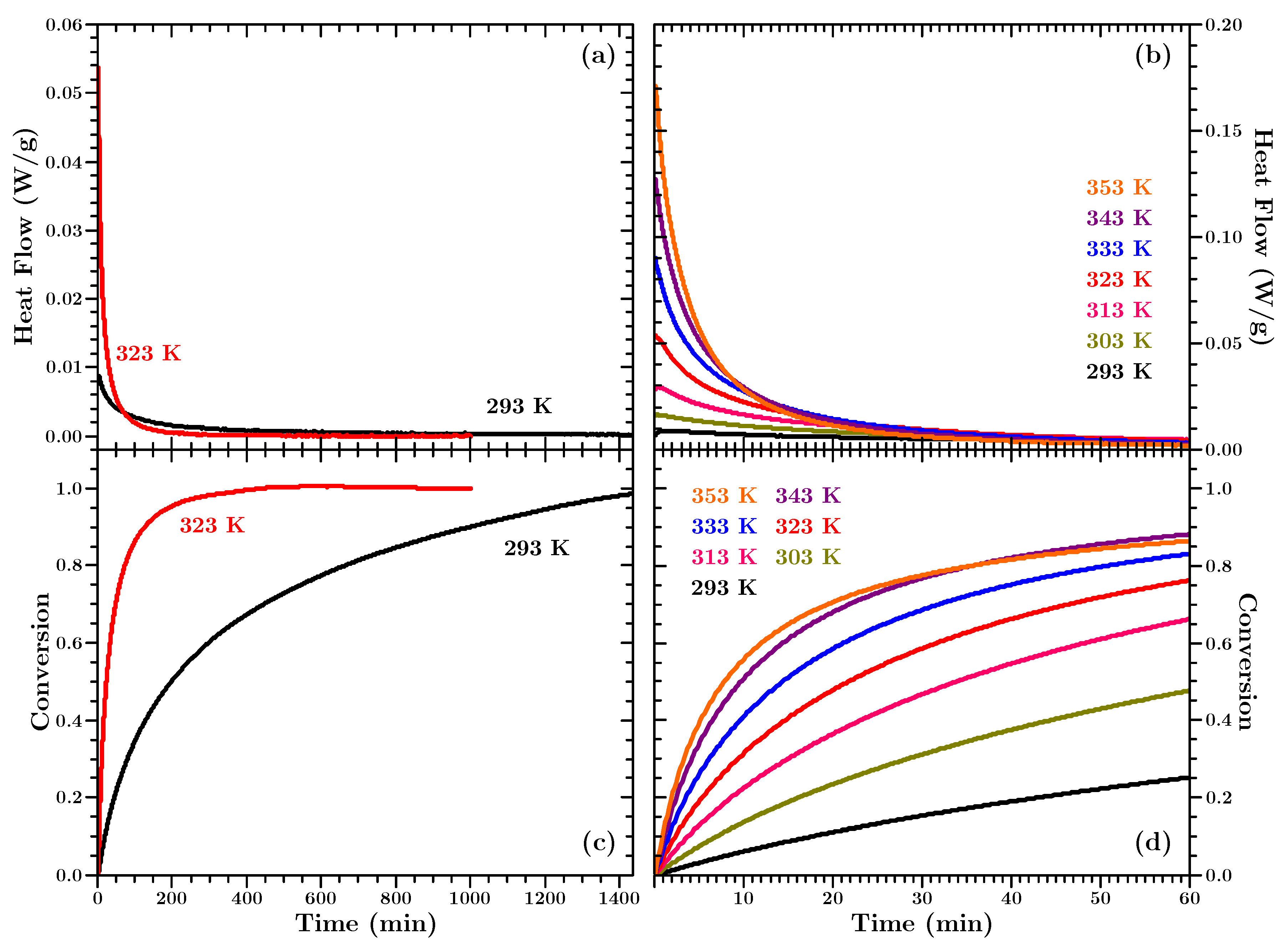
Figure 4 shows the measured heat flows and corresponding conversion (calculated according to Equation (
2); cf. also
Figure 1b) for the isothermal experiments.
The lower row of
Figure 4 shows that the material more quickly reaches higher conversion at higher temperatures, as was to be expected according to Equation (
1) since the Arrhenius term increases with higher temperature. Thus, at higher temperatures more heat is released early in the experiment, as the upper row of
Figure 4 shows. Hence, at lower temperatures the amount of heat released at any time is smaller than at higher temperatures, but heat is released over a longer period. This is shown on two heat flow curves in
Figure 4a. The heat flow signal for the experiment at 323 K falls below the heat flow curve for the experiment at 293 K after approximately 70 min. In the former experiment 100% conversion is reached after ca. 500 min and no heat flow is measured any longer, the signal reached the baseline level. In the latter experiment 100% conversion is not reached before ca. 2000 min.
As for the isothermal data
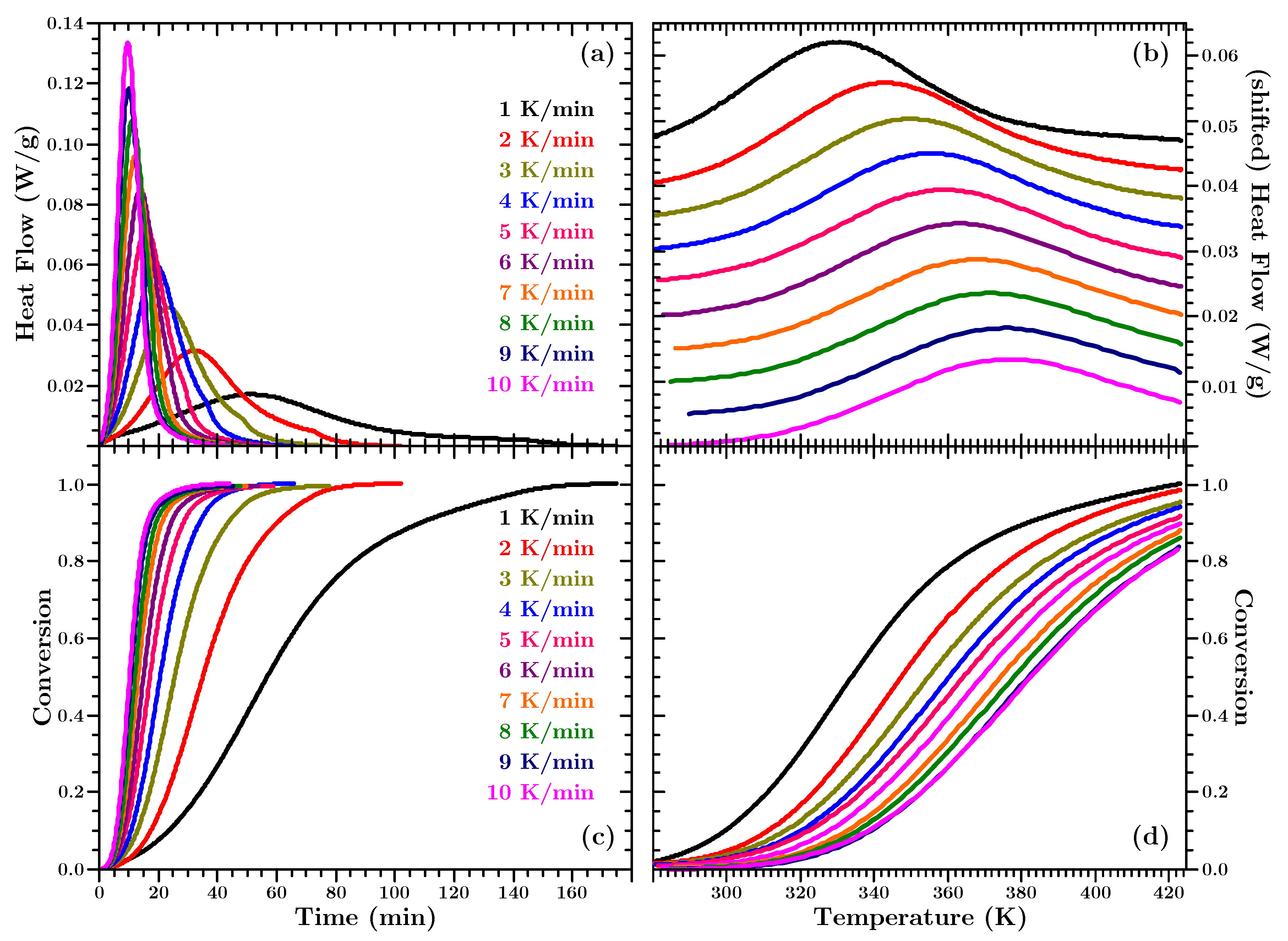
Figure 5 shows the heat flows and corresponding conversion for the dynamic experiments.
It can be seen that the position of the heat flow peak occurs at higher temperatures for higher heating rates. In addition
Figure 5 shows that the experiments do not reach full cure during the temperature ramps (with the exception of the experiment at 1 K/min).
The reason for the right shift of the peak in the temperature dependent dynamic data in
Figure 5b is the following: At slower heating rates the material spends more time at lower temperatures and reaches higher conversion earlier, temperature-wise (cf.
Figure 5d). The Arrhenius term in Equation (
1) still increases with rising temperature. Thus, the reason for a decreasing heat flow is to be found in
. As said above
is often assumed as the kinetic model to describe polyurethane. Hence,
decreases with increasing conversion. Temperature-wise, the heat flow peak occurs earlier in slow heating rate dynamic data, because the decreasing kinetic function “outpaces” the increasing Arrhenius term.
The isothermal and dynamic data shows quite different curing behaviour at different temperatures and heating rates. Any set of model parameters must be able to characterize this wide range of curing behaviour.
Table 3 presents the determined total heats of reaction for all experiments. The total heat is the integral of the curves shown in
Figure 4 and
Figure 5 (cf. also
Figure 1b).
As
Table 3 reveals, the total heats of reactions are all similar. For the isothermal values a mean value of 67 J/g was found, while it was 73 J/g for the dynamic experiments.
The scatter in the total heat values seems high (especially for the isothermal experiments), but is comparable (or better) to other reported differences in total heat values of thermoset resins from one experiment to another determined by DSC [
36,
42,
49,
75].
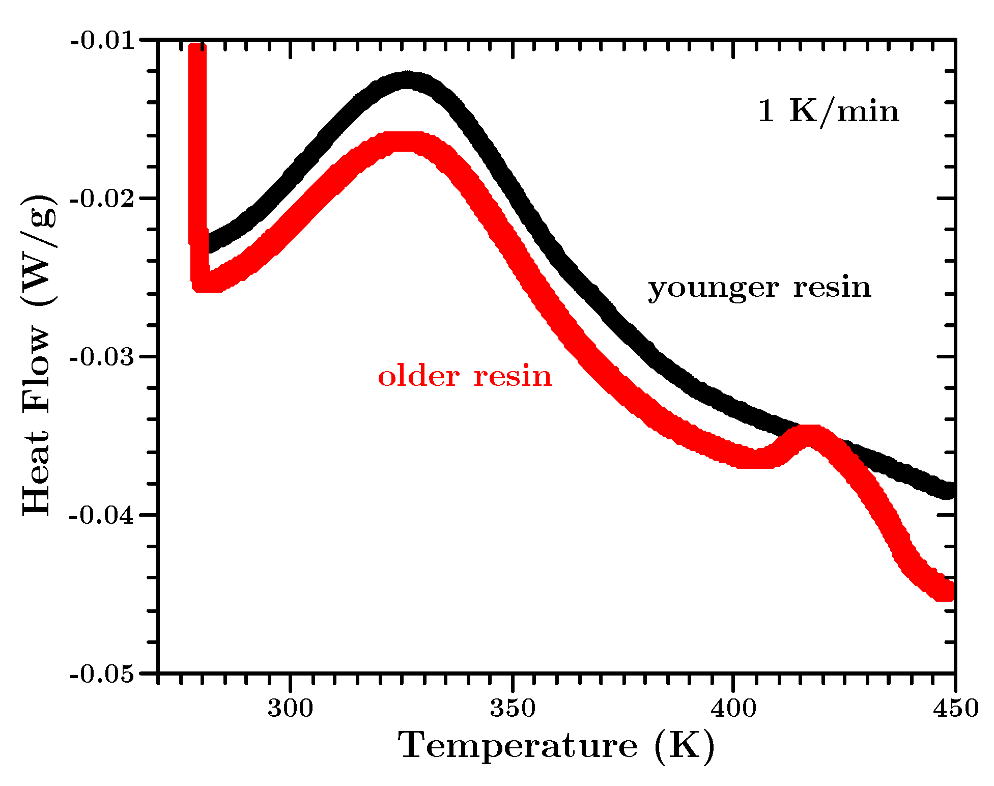
The mean of the dynamic total heat is slightly higher than for the isothermal data. This difference can be explained by a second, not curing related, small heat flow peak, which occurs at high temperatures (cf.
Figure A3). Since we measure just the sum of the heat flow of all different origins, we cannot distinguish it from the curing related total heat. However, this second peak does not occur at the temperatures at which the isothermal experiments were performed. Taking the concrete engineering application of this material into consideration this material is not supposed to experience temperatures above 353 K. Thus, we decided to use the mean of the total heat from the isothermal data. This experimental artifact is discussed in more detail in
Appendix E.
7.2. Heat Capacity
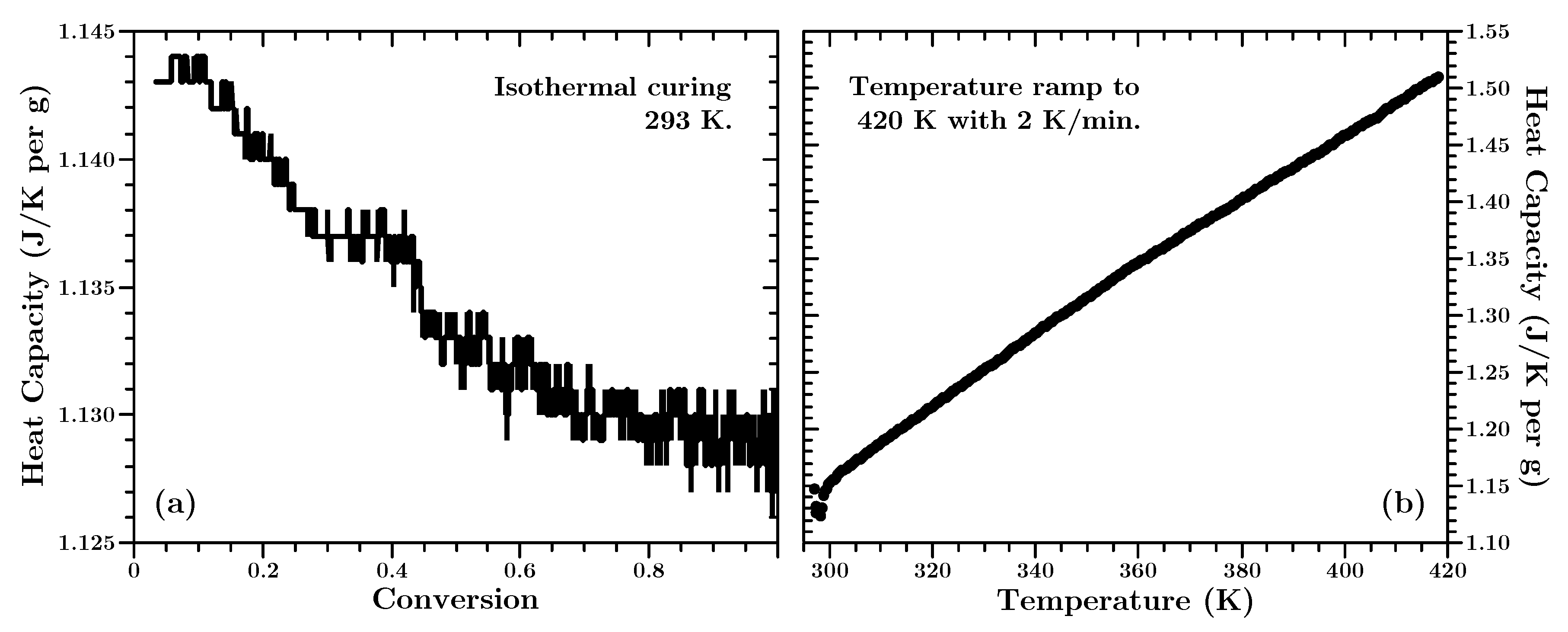
In
Figure 6 the conversion and temperature dependency of the heat capacity is shown. The latter is shown for the fully cured material (cf.
Section 5.1).
Figure 6 reveals two things. Firstly, the change of the heat capacity is approximately 1%. This is just slightly larger (about three times) than the natural variations of the measurement signal of the instrument. Thus the change in the heat capacity during the curing process can be justified as insignificant and is just visible due to the scaling of the ordinate. Secondly, the temperature dependence of the heat capacity
is almost perfectly linear:
Due to the high viscosity of the material (compared to neat resin) we assume that the amount of additional non-reactive fillers in the material is rather high and that the properties of the filler dictate the overall temperature behavior of the uncured and fully cured material. Non-reactive filler’s are common in industrial applications to lower the costs of a material or to tailormake the properties of a polymer [
76,
77]. The low conversion dependency of the heat capacity supports this assumption strongly. For an unfilled resin a heat capacity change between approximately 10 to 25% would be expected during the curing process, as reported for other thermoset materials [
44,
47,
48,
71,
72]. The constant heat capacity is beneficial for the analysis, since a straight baseline is assumed for the heat flow data (cf.
Section 2.1 and
Appendix C), which will not lead to large errors as long as the heat capacity does not exhibit a significant change during cure [
15,
55].
7.3. The Kinetic Triplet Determined with Regular Function Fitting
While the correct kinetic model of polyurethane is still a topic of academic debate, often a so called
n-th order model (cf.
Table 1) is used to describe the curing progress [
78,
79]. Regular fitting of the isothermal data according to Equation (
1) with
leads always to very good agreement between the data and the fitted curves and yields values for
A,
E and
n. However, these parameters are very dependent on the initial guesses for the fitting algorithm. Regular fitting of the dynamic data is more robust regarding the initial parameters, however, the determined activation energies and reaction orders are dependent of the heating rate which should not be the case. Thus one set of kinetic parameters determined for one heat flow curve do not describe a heat flow curve for a different temperature or heating rate. This was the reason why the authors employed the isoconversional apparatus to determine a kinetic triplet which describes all types of curing heat flow curves of this material.
7.4. Activation Energies Based on the Isoconversional Method
The activation energies, determined by Equation (
4) can be seen in
Figure 7.
Figure 7a reveals a more or less constant activation energy for
which is diverging above this value. Stanko and Stommel report in [
75] the same behaviour for fast curing polyurethane resins. However, no explanation is given why the activation energy diverges. We assume that the above mentioned second, not curing related peak in the heat flow data at high temperatures may be the reason. This peak does not occur at low temperature, thus not at low conversion. Therefore, at high temperatures a compound activation energy is determined—one value for the actual curing process and the process responsible for the second peak. In order to predict the heat flow (cf.
Section 7.7) it turned out that it is most practical to use a constant activation energy for
of 44 kJ/mol.
In
Figure 7b it can be seen that for
both types of datasets (isothermal or dynamic) yield virtually the same activation energy, as mentioned earlier. However, below 20% conversion the determined values for
differ slightly from each other, but never more than aobut 4%. Such differences in the activation energy for low conversion have been reported for other types of thermosetting polymers [
23,
80] and were attributed to changes in the viscosity of the material. However, investigations of the issues around this matter would require more experiments and are out of the scope of this article, especially considering that the differences are rather small.
The temperature in a large cast of the material would not be expected to rise as fast as is characteristic for the dynamic experiments, as already mentioned above. It is however expected that stepwise isothermals in a simulation describe the material more accurate. Hence, the development of the activation energy was described with a second order polynomial
which was used to predict the heat flow and in the simulations presented below.
Lastly, it shall be mentioned that the determined activation energies are not dependent on the initial guess used to minimize Equation (
4). Thus, one of the problems in connection with regular fitting is solved by the isoconversional method.
7.5. Determining the Pre-Factor
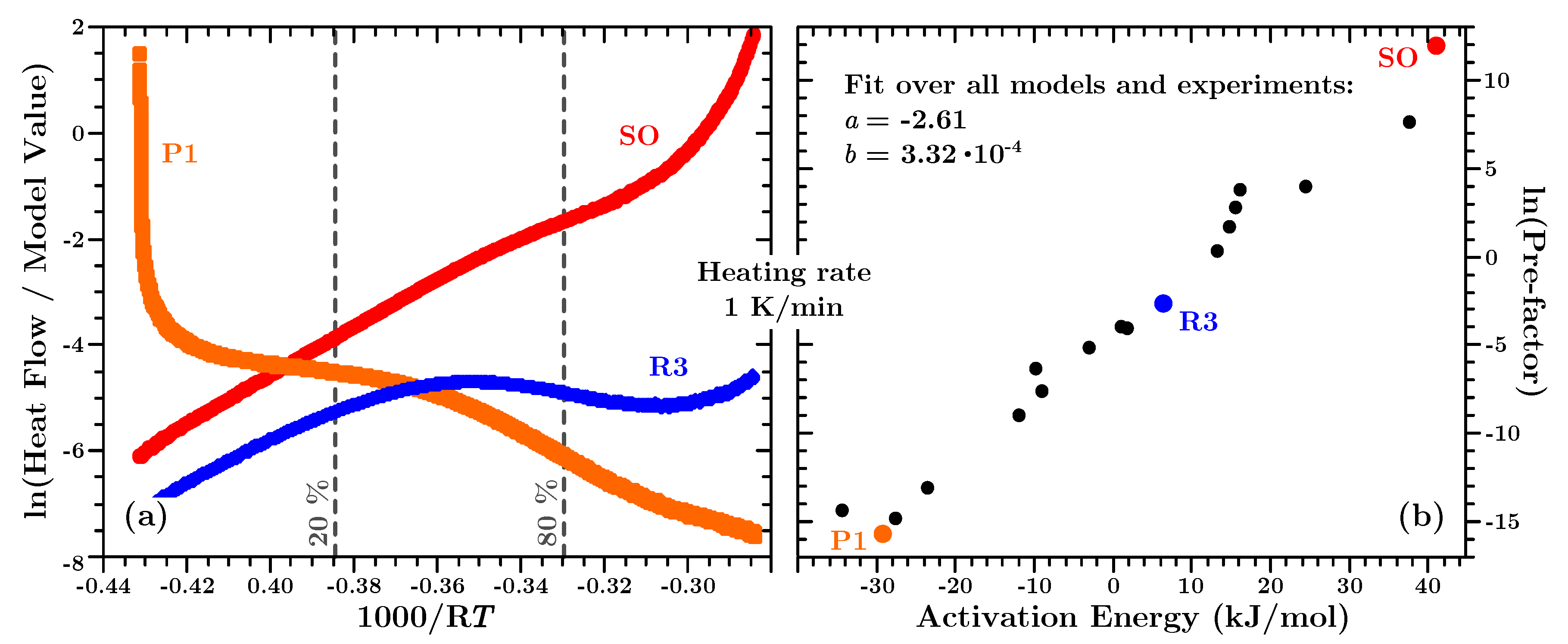
In
Figure 8a the functional value of the left side of Equation (
7) is plotted for a second order kinetic function—
, a power law—
and a contracting sphere model—
(cf. also
Table 1).
If these kinetic models (and all others in
Table 1) are fitted between
as described in
Section 3.2, the sets of pre-factor and activation energies are found as shown in
Figure 8b. Indeed, a linear relationship exists between these values, as described in Equation (
7). When all dynamic experiments are fitted in this way with all kinetic models in
Table 1, a linear fit over all these
and
yields the compensation parameters
J/mol and
.
It is beyond the scope of this article to interpret the compensation effect itself. Its origin remains the subject of academic debate and several mechanisms were proposed as towhy it exists at all [
81,
82]. Qualitatively the same results were reported in the references cited above for many material systems and processes. Hence, we accept it as consensus that the compensation effect is real. Due to the convienence of its simplicity, the compensation effect fits very well with the scope of this article.
The determined compensation parameters are independent on the dataset used for the calculations. Thus, the second problem of regular fitting, one set of parameters not valid for all datasets, was solved by employing the compensation effect to determine the pre-factor.
7.6. The Actual Kinetic Function
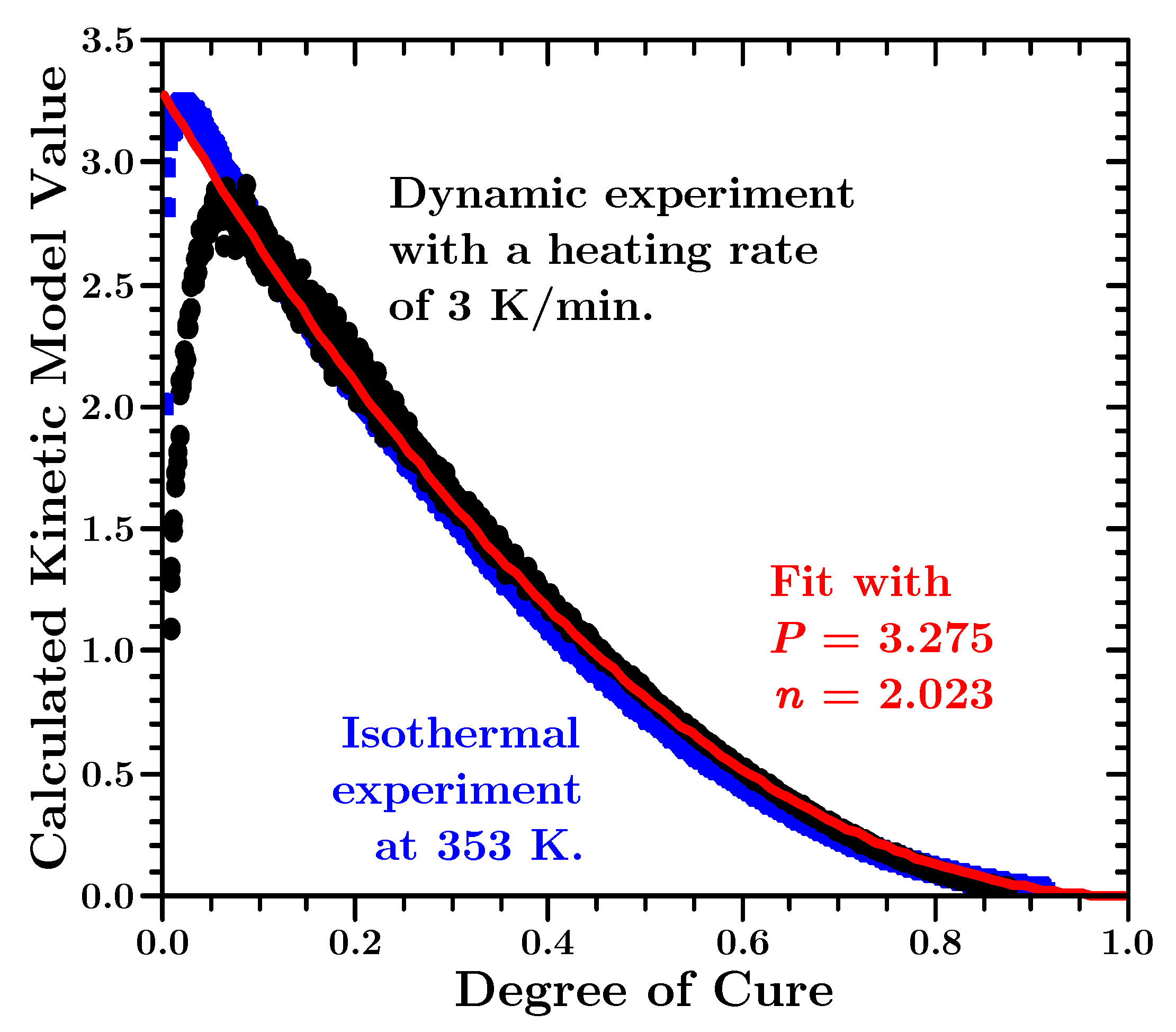
In
Figure 9 the actual kinetic function
, calculated from Equation (
9) with two representative datasets, can be seen.
The values of the black points in
Figure 9 were calculated using a dynamic dataset, whereas the values of the blue squares were calculated with an isothermal dataset. These two curves are representative for all the kinetic functions, calculated with the data from the ten dynamic or the seven isothermal experiments. All the functions in
Table 1 were compared to these values. But as expected, the kinetic function is best fitted with a
n-th order equation, ignoring the first 6%. However, the
n-th order equation has to be multiplied with a factor, which we call
P:
The values of
and
are the mean values of the parameters determined by fitting all actual kinetic functions, that were calculated using the dynamic datasets, and fitting them for
with Equation (
13).
As already mentioned, the shape and magnitude of the kinetic function was little influenced by the concrete set of activation energies (isothermal or dynamic) used to calculate it.
A
n-th order equation does not fit the calculated kinetic functions below 6% since said equation can not reach a value of zero if
approaches zero. An autocatalytic kinetic model, such as a Sestak-Berggren equation (cf.
Table 1), could fit such a behaviour. However, the shape and maximum value of such a function did not agree with the data as well as the
n-th order equation that was finally used.
At this point the user of the above described method has to decide how much effort she or he intends to put into determining the true kinetic model. Stanko and Stommel, for example, used the more complex 3D diffusion model for fast curing polyurethane resins [
75]. In principle no additional experiments are needed to determine a more accurate description of the actual underlying chemical model. However, for the more practical approach of this article, ignoring the first 6% of conversion and using the
n-th order Equation (
13) is better suited. This is especially true in view of the good results of the simulations presented below.
7.7. Prediction of the Heat Flow
To test the validity of the results, the heat flow in the DSC experiments was calculated every 0.1 s according to Equation (
1) and with the determined kinetic triplet as presented in the previous sections. The only additional parameter used for these predictions was the exact total heat to make a comparison of the predicted and measured values meaningful.
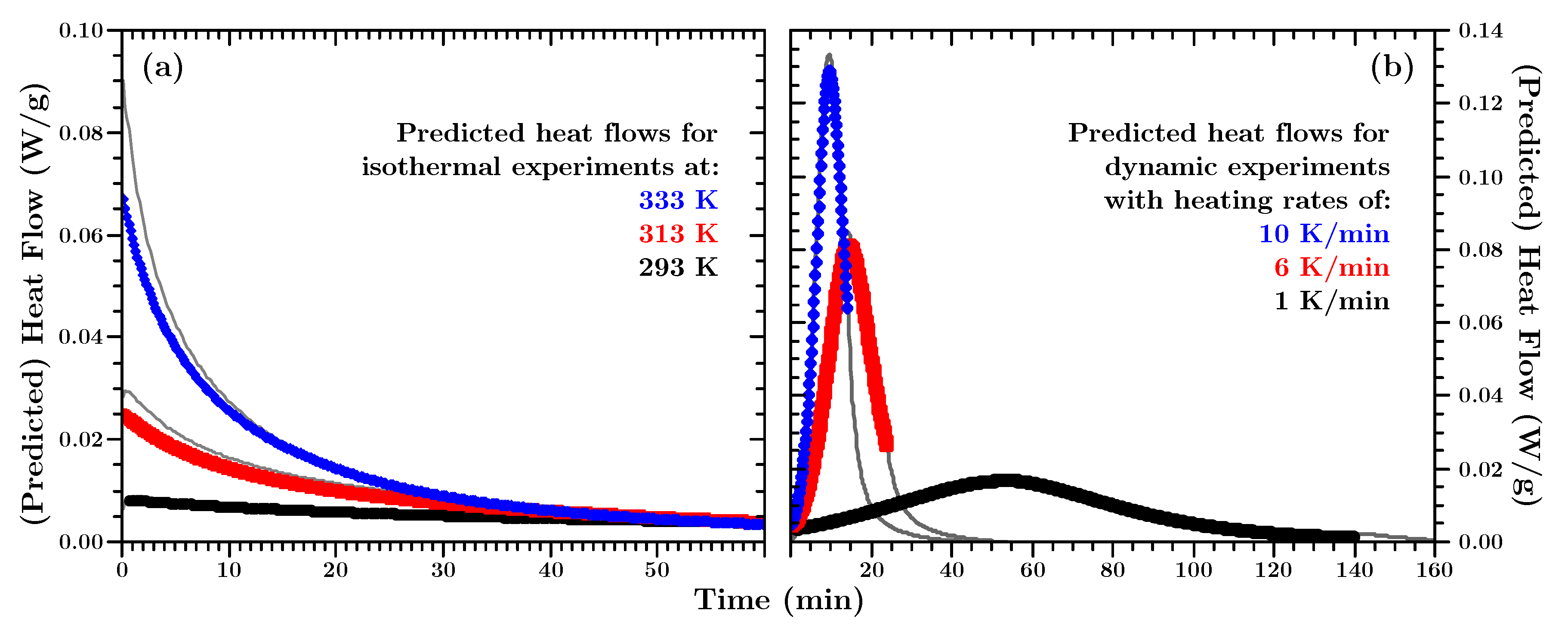
Figure 10 shows some representative predictions.
Since the predictions describe the DSC results from which the model parameters were obtained, good agreement between measurements and predictions is expected. However, considering all the modeling assumptions and simplifications made, it creates confidence in the modeling approach when the data match.
Even though only mean values were used, predicted and measured values agree very well. For isothermal predictions (
Figure 10a) the experimentally measured values are ca. 10% higher than the predicted values in the beginning of the curing process. The project partner from which we got the material assumes that minimal amounts of reaction accelerating chemicals may be part of the resin or hardener. Once the (assumed) supply of accelerators is used, the chemical reaction behaves according to the proposed model. However, this discrepancy becomes smaller within the first couple of minutes of the reaction.
The predicted dynamic heat flows (
Figure 10b) were performed only while the temperature increased. Here too, the predicted and actually measured heat flow values agree with each other.
The above predictions were made with the exact total heat values for each experiment to allow comparison between model and actual measurements. If the isothermal mean total heat value is used, as for the finite element simulations below, the differences are so small that the curves could not be distinguished from each other in
Figure 10. However, a detailed analysis reveals that the maximum relative error is ca. 10% or better at the position of the curve(s) where the two predictions deviate most from each other.
7.8. Simulation of and Actual Temperatures in a Cast Polymer Block
In
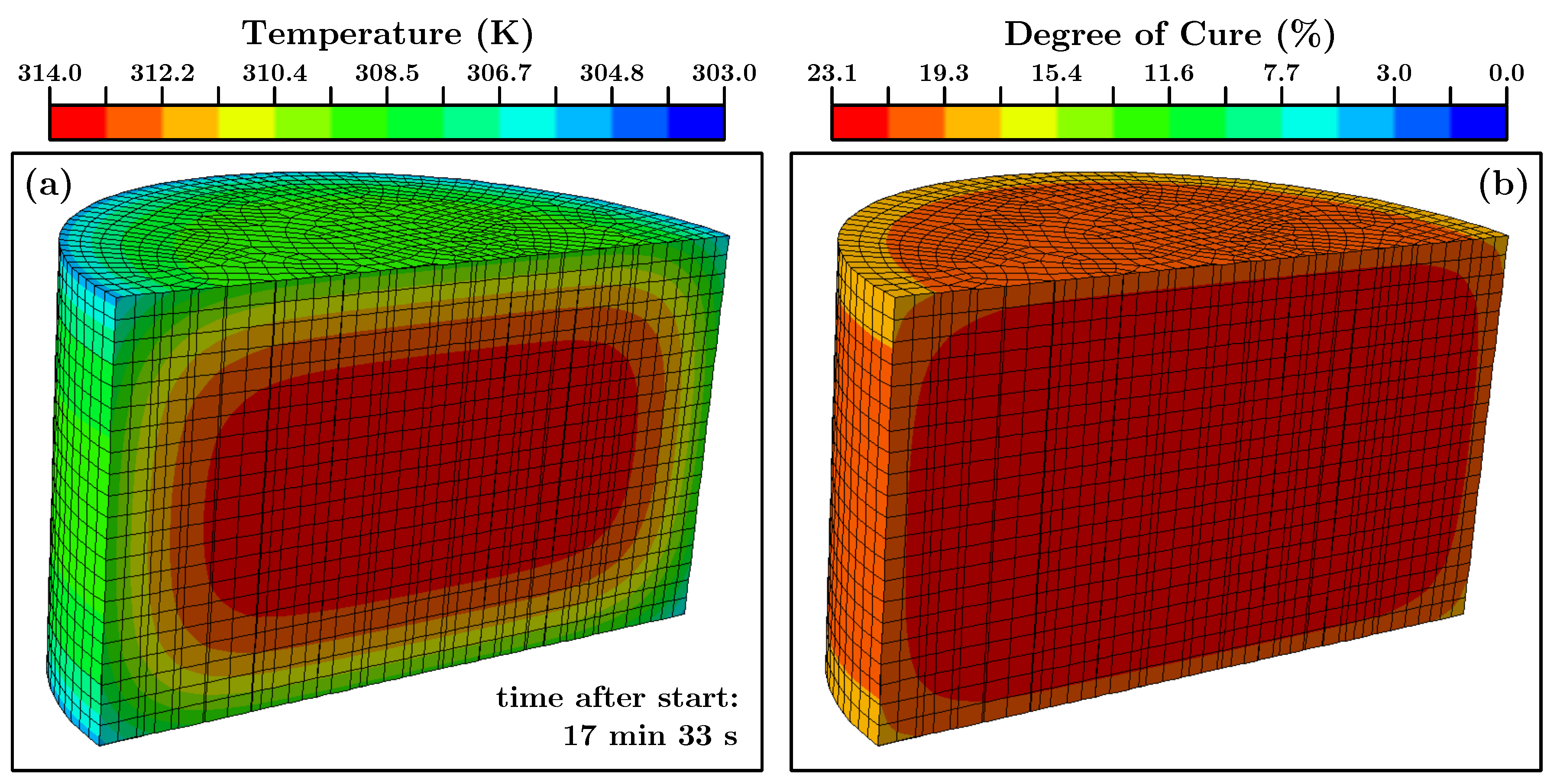
Section 7.7 the actual total heat of each experiment was used to make the heat flow predictions and the experiments more comparable. For the finite element simulations however, the mean value of 67 J/g was utilized. As described in
Section 6 we did first a finite element simulation of the material in the bucket after mixing the components. In
Figure 11 the results for one step can be seen.
The time step of the shown finite element simulation is 17 min and 33 s since this was the moment when the core of the simulated cylinder reached the value of the very first temperature measurement (ca. 314 K). At this point the degree of cure of the core (
Figure 11b) was ca. 23%. This value was used as the input parameter for the simulation of the curing process in the actual mold which contained the temperature sensors (cf.
Section 5.3 and
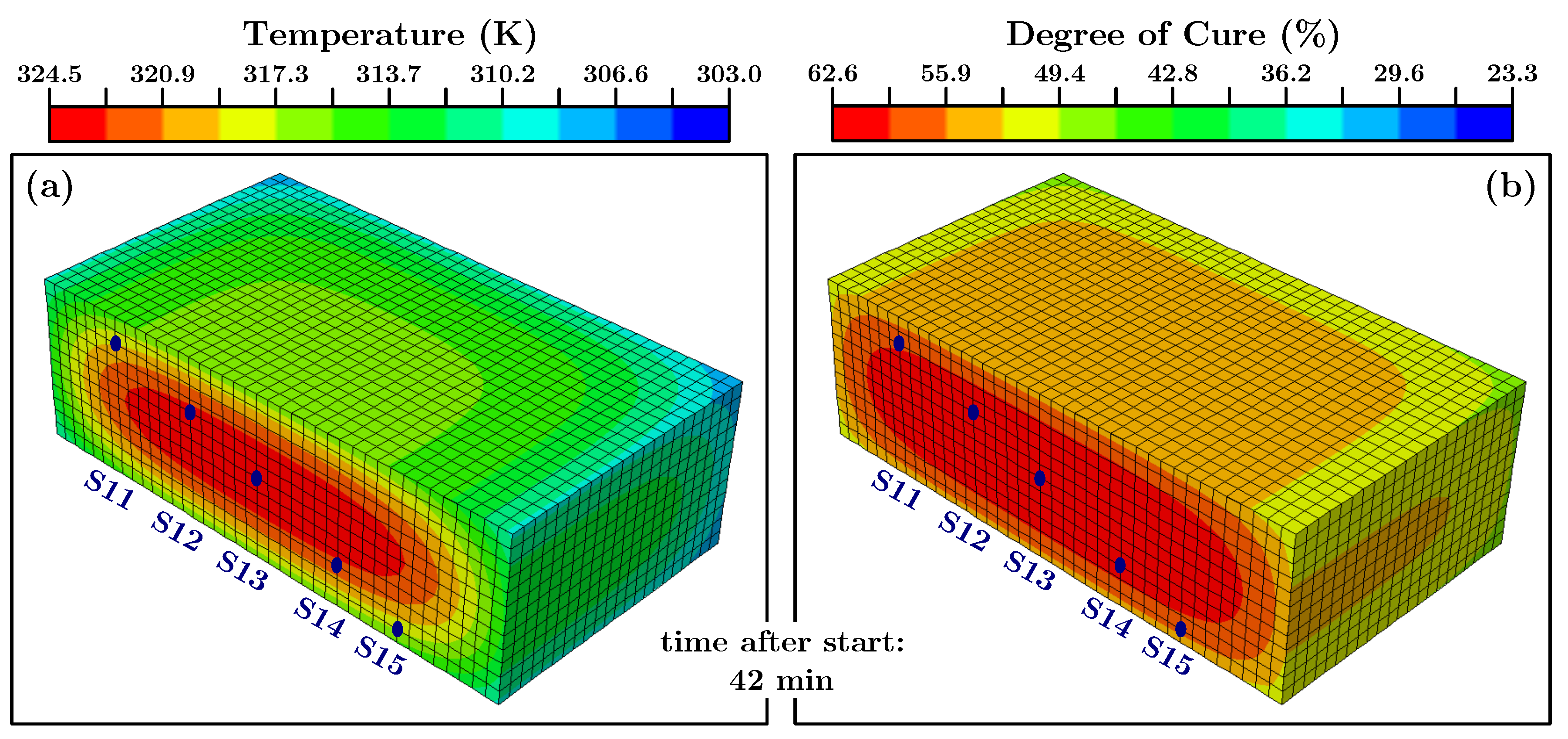
Figure 3). One step of these simulations can be seen in
Figure 12.
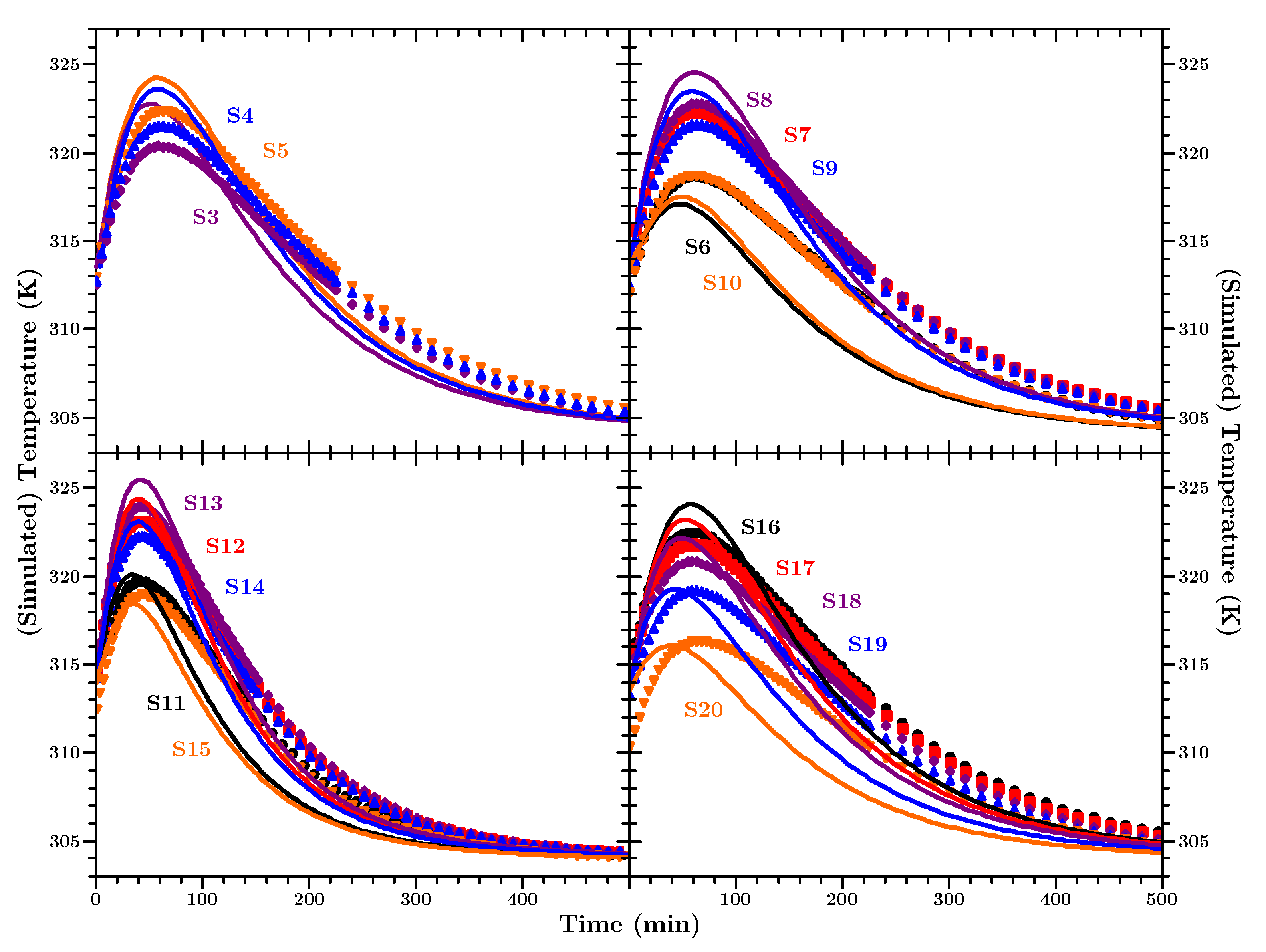
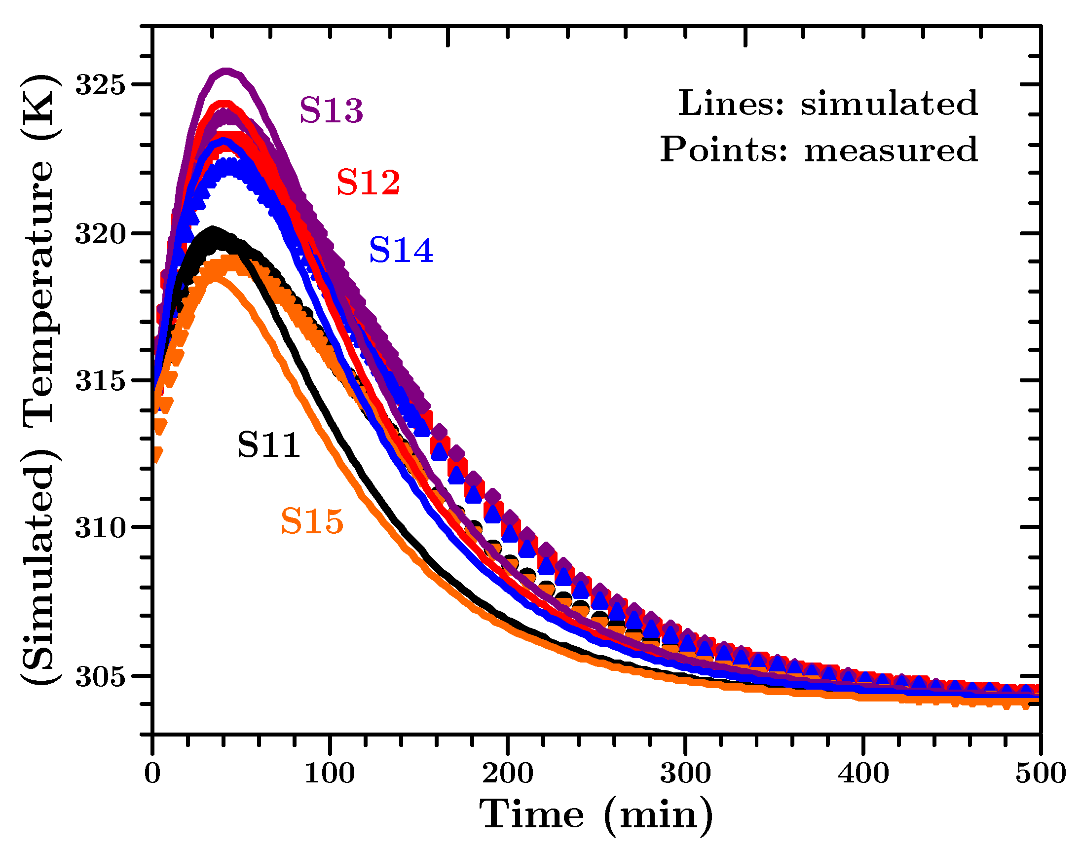
Since the conversion can not be measured directly, in-situ, in a large body the temperature development has to act as a proxy for information about the ongoing curing progress. In
Figure 13 the measured and simulated values of sensors 11 to 15 are shown.
The presented measurement values and simulation curves in
Figure 13 are representative for the experiment/simulation. The data of all temperature sensors is presented in
Appendix F.
Taking into account the uncertainties about the material and that mean values from the above described investigations were used, it can be stated that the measured and simulated temperature values agree well with each other. The most interesting period during the cure, for engineers to identify hot-spots in the material, is the period when the temperature is rising and when it reaches its highest value. The simulation predicts the peak temperatures within an error of max. 3 K. In addition the (time wise) peak positions and the differences for sensors at different positions are predicted very well. The simulated body cools slightly faster than the actual material in the experiment, but the overall dynamic of the temperature development is predicted correctly over three orders of magnitude in time. One minor disagreement can be seen between the simulated temperature and the actual measured temperature. From a purely physical point of view, the material closer to the edges of the block (e.g., sensors S11 and S15) should exhibit the temperature peak earlier than the material in the middle of the block; simply due to the closeness to the colder outside. The underlying physical model of the finite element heat transfer simulation predicts this correct. However, we observe a slight difference between the peak positions of the measured and predicted temperature values. For the measured values the shape of the temperature curves seems to follow the core temperature, and the temperature peak occurs for all positions at the same time. We have to admit that we do not have an explanation for this behaviour. However, it has also been observed in a different kind of thermosetting polymer [
83]. Apart from that, the amplitude of the predicted temperature agrees well with the measured values at all positions. Since, from an engineering perspective, the prediction of the temperature values is most important and because the deviation in the peak positions is only by minutes (in an experiment over a day) we consider the simulations a success.
8. Discussion
The results have shown that the kinetic triplet describing the curing of a polymer can be obtained by straightforward experimental DSC measurements. The parameters for the kinetic triplet of the polyurethane polymer studied are summarized in
Table 4.
This set of parameters describes all measured data equally well. The parameters are used as input to finite element analysis for predicting curing of cast components.
The procedure described here allowed finding a consistent set of parameters. The activation energy was obtained based on the isoconversional method, the Arrhenius pre-factor was determined using the compensation effect and the kinetic function was obtained by comparing the actual kinetic function calculated with the correct activation energy and pre-factor with known kinetic models for polymers. Regular curve fitting was than used to determine the parameter P and n of said kinetic function.
The equations to obtain the parameters are simple as shown in the previous sections. However, performing all the required calculations against experimental data is substantial and can be considered as not trivial. Computer programs need to be created to make the data analysis possible. However, this is a rather simple task and commercial software exists for free, and open source programs can be found online in the common software repositories.
Simplifications were made either to analyze the data and for the final finite element simulations.
A straight heat flow baseline was assumed. The baseline corrected heat flow data was obtained by simply subtracting the post-cure run data from the cure-run heat flow data.
Mean values were used for the total heat , the compensation parameters a and b, and the parameters P and n of the kinetic function, as stated above.
A n-th order kinetic function was used for , which is one of the simplest models to describe the curing of a polymer.
The first ca. 6% of the calculated actual kinetic function were omitted to arrive at said conclusion that the reaction can be described with a n-th order kinetic model.
The choice of these simplifications is mainly justified by the success of modeling the generated heat and temperature of the DSC experiments and of a cast big block. The predicted temperature and heat of the DSC tests match the measured values well, regardless of if a slow isothermal reaction at 293 K or a fast dynamic experiment with a heating rate of 10 K/min are predicted. The former needs many hours and exhibits rather small heat flow values while the latter reaches 100% conversion in a matter of minutes and develops heat flow values more than a magnitude larger. The simulation of a large cast of said material predicted the location dependent magnitude and the trend of the temperature within an accuracy of 3 K. Thus, despite the simplifications the above-described methods give relatively precise predictions.
Since the analysis based on the isoconversion method is an integral method, the influence of the natural variations between experiments is minor and the determined model is good enough for engineering purposes. For example, the prediction of the isothermal heat flow is systematically underestimated by about 10% for the start of the reaction, but the overall prediction is still good.
It should be noted that it was not possible to find a consistent set of parameters using the standard DSC analysis based on regular function fitting. Ambiguous kinetic parameters were obtained, valid for only one dataset, but not another.
It is possible to evaluate each of the kinetic triplet parameters in more depth and more accurately. Some indications on how this can be done were described earlier. But the goal of this study was to describe the degree of curing and the heat of curing during the molding process of components. A more detailed description of the individual processes does not necessarily improve the prediction of the progress of the curing of the material. Discrepancies between the model and reality appear mainly at low curing rates and very high curing rates. Both are not so critical for most molding processes. At low conversion the polymer is still close to being liquid. At high conversion the curing process is essentially finished anyway.
The approach described here should be applicable to many other polymers than the filled polyurethane that was described here. One assumption made in this work was that the heat measured during the DSC tests is not influenced by a phase transition. If this approach is applied to an epoxy resin, this may not be right. The temperature of the epoxy may cross the glass transition temperature during curing. In this case the baseline correction would get somewhat more complicated. If modulated temperature DSC is used to monitor the dependency of the heat capacity from the conversion [
44,
71], the baseline can be reconstructed [
55]. Since the temperature dependent heat capacity is also needed for simulating the heat development during the cure at least one temperature modulated DSC experiment should be performed. In contrast to polyurethane, the cure of epoxy is usually described with kinetic models containing more than one reaction pathway, and thus more than one reaction rate coefficient. However, it has been shown that the isoconversional method can also be applied to determine the kinetic parameters in such cases [
23,
24,
26,
27,
80].
If the kinetic triplet of a new polymer shall be investigated it is sufficient to perform only the dynamic tests with a DSC. However, the authors feel that double checking of the activation energy with dynamic and isothermal data is advantageous.
Many material properties are dependent on the degree of cure. Thus, calculating the degree of cure is relevant for many applications and control of production processes. For example, the development of the (cure) shrinkage of a polymer can be determined by e.g., embedding optical fibers into the liquid material and monitoring the strain during the curing process [
83]. Then another simple Abaqus user subroutine (UEXPAN) can be used to simulate said cure shrinkage, allowing more insight into the characteristics of a large polymer cast. This illustrates that the isoconversional method as described above stands just at the beginning of further possibilities.
9. Conclusions
The prediction of the degree of cure, the associated heat and temperature increase during the curing of a polymer was successfully done using a standard finite element program with the so called “kinetic triplet” as input parameters. The kinetic triplet consists of the activation energy, the Arrhenius pre-factor and the kinetic function, which describes the chemical reaction. The three parameters could be obtained with standard DSC equipment. The data were analyzed with the model-free isoconversional method combined with the compensation effect. The same set of parameters allowed prediction of cure behavior over two orders of magnitude of time and at a curing temperature range from room temperature up to 420 K.
The parameters obtained with this method were checked against DSC data and more importantly, the curing of a large polymer block of mm3. Agreement between the simulations and measurements for the (DSC) was within a relative error of ca. 10%. Temperature measurements in the large block were accurate within 3 K. The timing of the peak temperatures was predicted within 3 min in the core of the block and 9 min at its edges, while the whole simulation spanned more than 13 h.
The overall process can be easily applied and can be summarized in the following few steps.
Perform a number of dynamic DSC experiments (cure + immediate post cure) to gather the heat flow raw data.
Subtract the post cure data from the cure data to get the correct baseline and heat of reaction.
Calculate the kinetic parameters. The paper gives the required equations to determine the total heat(s) of reaction, the activation energy via the isoconversional method, the pre-factor via the compensation effect and the actual kinetic function.
Said actual kinetic function needs to be compared to existing models or parameterized individually.
All the gathered information can then be used in a simple finite element simulation with a program of the user’s choice.
Some simplifications were made when describing the parameters characterizing the cure reaction. The simplifications were important to reduce the computational effort and to make the method applicable over a wide range of application cases. Due to the integrating nature of the analysis these simplifications do not reduce the accuracy of the predictions significantly, which was confirmed by good agreement with the experiments.

