An AWS Machine Learning-Based Indirect Monitoring Method for Deburring in Aerospace Industries Towards Industry 4.0

Featured Application

The proposed method could potentially be applied to aerospace manufacturing industries or other manufacturing processes that required in-process sensing to monitor the quality of the component or part.

Abstract

The number of studies on the Internet of Things (IoT) has grown significantly in the past decade and has been applied in various fields. The IoT term sounds like it is specifically for computer science but it has actually been widely applied in the engineering field, especially in industrial applications, e.g., manufacturing processes. The number of published papers in the IoT has also increased significantly, addressing various applications. A particular application of the IoT in these industries has brought in a new term, the so-called Industrial IoT (IIoT). This paper concisely reviews the IoT from the perspective of industrial applications, in particular, the major pillars in order to build an IoT application, i.e., architectural and cloud computing. This enabled readers to understand the concept of the IIoT and to identify the starting point. A case study of the Amazon Web Services Machine Learning (AML) platform for the chamfer length prediction of deburring processes is presented. An experimental setup of the deburring process and steps that must be taken to apply AML practically are also presented.

1. Introduction

The Internet of Things (IoT) was first introduced by Kevin Ashton in 1999 [1]. He proposed the concept to bridge physical and virtual objects through a network of sensors and computers. This allows for the direct and indirect exchange of data between devices and applications. A review of the definition of IoT from the literature is presented in Reference [2]. Amazon Web Services (AWS) defines the IoT as a managed cloud platform that allows devices to be easily interconnected to each other and for them to securely interact with cloud applications and other devices. A simple definition from our perspective is defined as follows: IoT is the way to transform raw data, which is obtained from the environment of physical systems, into useful data that can be used for monitoring purposes or decision-making by means of the internet, cloud computing, and intelligent systems.

The IoT has been applied in various fields such as the fields of social sciences [2], healthcare [3], food supply chain (FSC) [4], and transportation [5]. A more detailed view of IoT applications in other fields such as the fields of logistics, smart home and buildings, smart cars, energy, safety and security, governance, education, and entertainment has been reviewed quantitatively in Reference [2]. In this paper, the application of IoT is narrowed down to industrial IoT (IIoT), especially in the manufacturing engineering field.

During the October 2017 AWS public sector SUMMIT in Singapore, AWS mentioned that the IoT comprise of three pillars, namely, (1) things, (2) the cloud, and (3) intelligence. Without cloud computing and intelligent systems, the IoT is merely the transference and communication of data through the internet. This paper presents a preliminary study on cloud computing and an intelligence-based machine learning method for industrial practices.

The cloud computing services hype began in 2006 when Amazon first established Amazon Web Services for small-scale developers to test their applications. Cloud computing services have now dominated the software application field due to their ability to hyper-scale the size of a project.

In recent years, the development of advanced mechanical systems and manufacturing technology has been on a path of continuous high demand with more specifications due to the need for better and more consistently high-quality products, more product variability, a reduced production cost, globally competitive products, and a shorter product life cycle. The advancement of data communication and storage through the IoT leads to possibilities of connecting sensors, robots, and devices.

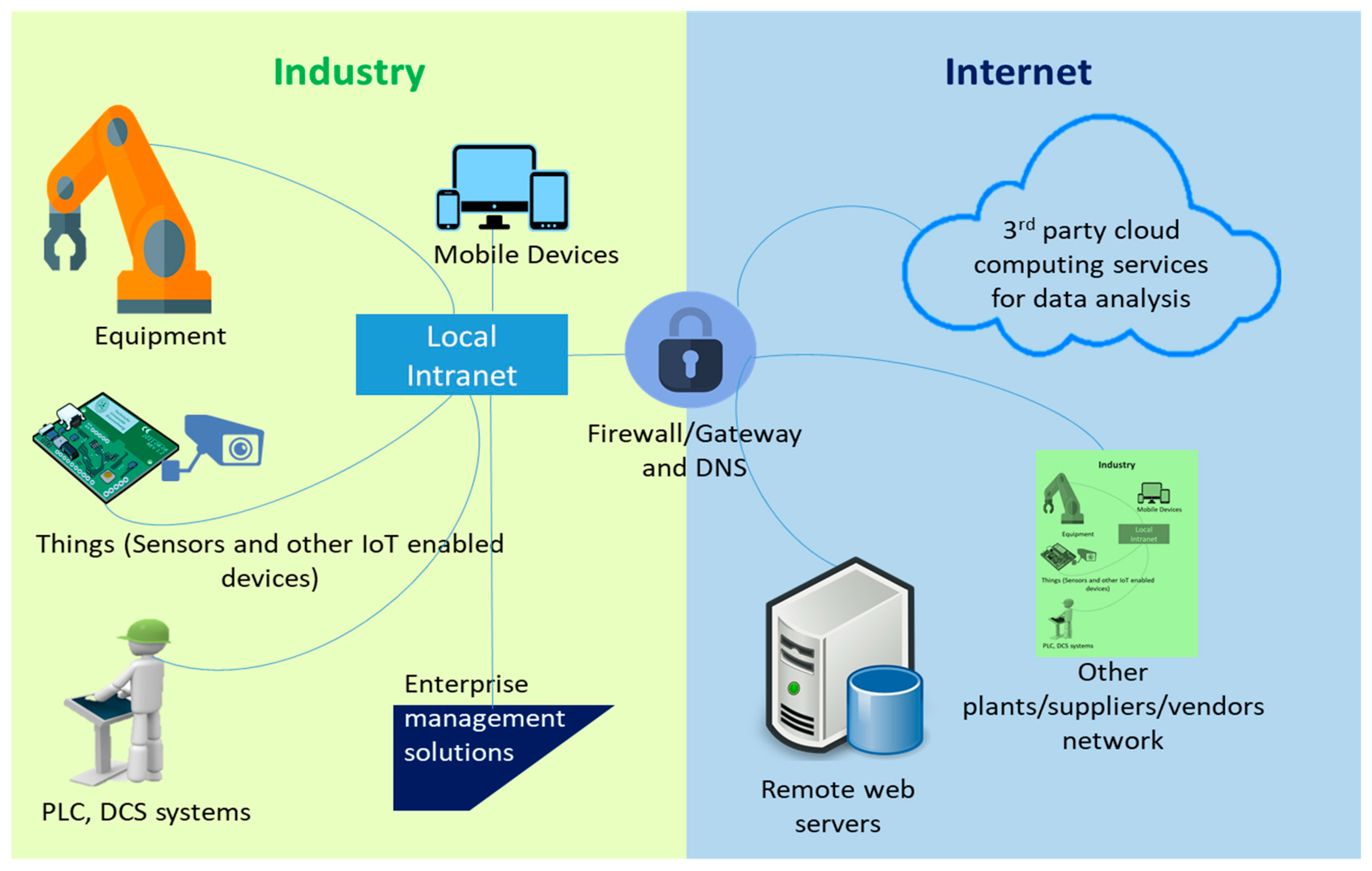
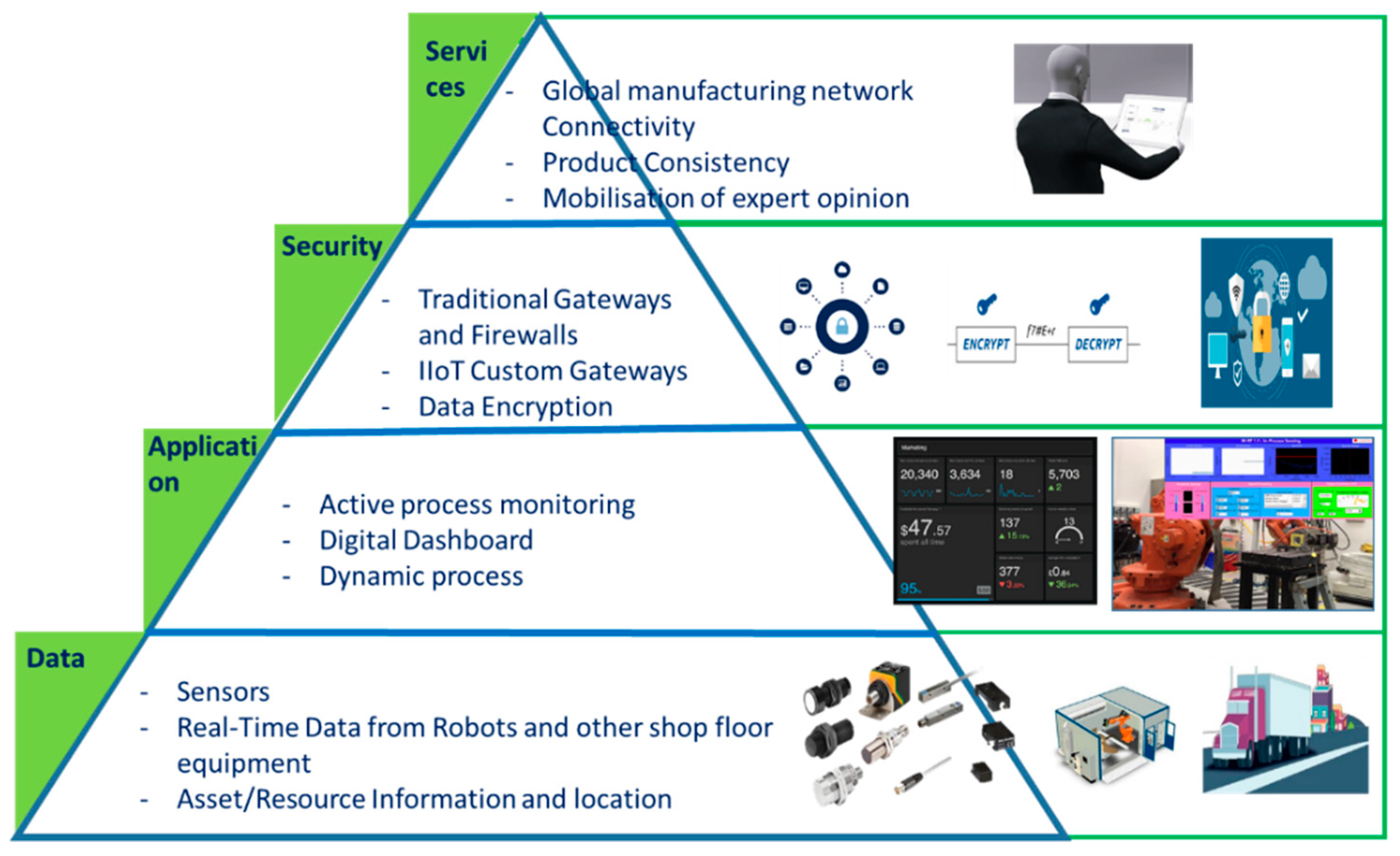
The current manufacturing scene consists of advanced automation technologies using robots and implementing an IoT architecture. This set-up requires the integration of intelligent data processing sensors and state-of-the-art machine-to-machine (M2M) technologies with existing automation technologies. Such an architecture is required to utilize IIoT or the industrial internet in the manufacturing industries. The convergence of industrial internet infrastructures with the advent of IoT technologies can be further illustrated in Figure 1.

This paper presents a brief review of IoT applications from the perspective of the manufacturing field in order to provide significant information so as to initiate the IIoT applications. The review particularly concentrates on engineering applications rather than from the computer science perspective. The study of AWS machine learning is also validated by means of the application of the post-manufacturing process, where the goal is to predict the quality of the component using AWS-featured machine learning. This method is potentially applied to enhance the conventional measurement method in aircraft manufacturing industries.

Our research motivation is to study the implementation of AWS Machine Learning (AML) in practical applications in the aerospace manufacturing industry, especially in the surface finishing process. The challenge of this study is to succeed in secure data transference and storage because the aerospace industry is strictly concerned about the secure communication and transfer of data to the external servers.

The paper is organized into 5 Sections. The motivation and IoT definition is presented in Section 1. The architectural design of the IoT is described in Section 2, which is comprised of 4 layers, i.e., the data layer, the application layer, the security layer, and the service layer. Section 3 explains the role of cloud computing in the IoT. This role includes cloud computing services such as Infrastructure as a Service (IaaS), Platform as a Service (PaaS), Software as a Service (SaaS), and the vendor option. An example application of AWS machine learning (AML) used to predict the quality of the components in the surface finishing process is presented in Section 4. In addition, Section 4 presents a detailed view of the AML features and the steps that must be taken to implement the AML so as to predict the chamfer length in the deburring process. Finally, the research conclusions, potential improvements, and future work are presented in Section 5.

2. Architectural Design of IoT

To initiate an IoT application, a certain data architecture design has to be predetermined. In the data architecture, a flow process that transforms raw data into useful data can be obviously seen. The architecture also enables us to understand what kind of software and hardware are necessary to build the IoT application. The following is a brief review of some proposed IoT architecture.

A recent survey on the IoT in the industry mentioned that the International Telecommunication Union recommends that the IoT architecture should consist of five different layers, i.e., the sensing, accessing, networking, middleware, and application layers [6]. In addition, the authors in Reference [6] proposed a service-oriented architecture for industrial applications from the perspective of the functionalities of the four layers, namely, the sensing layer, the networking layer, the service layer, and the interface layer. In another review paper [7], the authors presented a three-layered architectural model for the IoT, which consisted of the application layer, the network layer, and the sensing layer. In one example in healthcare applications, the author proposed three major layers, i.e., the perception layer, the networking layer, and the service layer (or application layer) [3]. In a more relevant article to manufacturing processes that involved a lot of sensors, Liu [8] proposed four layers comprising the physical layer, the transport layer, the middleware layer, and the application layer for sensory environments. According to the abovementioned reviews, a potential IIoT architecture for the manufacturing process is proposed as illustrated in Figure 2.

In an industrial setting, the standard IoT architecture will serve as a rigid option and a more requirement-specific adaptation of the architecture becomes necessary. We consider the lowest layer as ‘data’, however, the data generated from the shop floor (as can be seen in Figure 1) will not exclusively be from physical sensors. The data will consist of sensor data, asset particulars, and images and information pertaining to the operator. Hence, generalising the lowest layer as a sensing layer is inadequate. The data acquired from various sources have to be classified with the metadata, while a preliminary assessment to derive the conclusions/predictions must be performed. A Human-Machine-Interface (HMI) and an application of the programming interface must be developed to fulfil this requirement. This can be classified under the ‘application’ layer. Another important consideration in such a scenario is safety. As the security of data generated within the industry and the shop floor is very crucial, adequate measures to ensure the safety of the data should be accounted for in the architecture itself. This brings us to the third proposed layer: ‘security’. In sequence, following data acquisition, process monitoring, and adequate encryption, the architecture can be packaged into a ‘service’ in such a way as for the coherent information from the data to be easily understood by other personnel associated with supervisory and monitoring duties relating to the manufacturing process. This would improve productivity as any abnormal process behaviours can be predicted and, therefore, mitigated, hence, reducing equipment downtime [9].

2.1. Layer 1: Data Layer

The data layer can be associated with the process of identifying data sources and acquiring relevant data from these sources. For applications involving prognostics, the data acquired from past instances are also grouped under this layer. In order to acquire data from the sensors, standard data acquisition (DAQ) devices should consider the wide band of the sensor in order to avoid any data losses. The IoT-enabled asset tags will help to acquire information with regards to the asset location and availability. The data layer essentially includes all the data regarding the identified ‘things’ on a manufacturing floor.

2.2. Layer 2: Application Layer

The application layer acts as the medium to access the process-related data. This can be interfaced by off-the-shelf systems like distributed control systems or custom data interfaces. Some of the current manufacturing processes are equipped with process monitoring solutions and these applications enable the shop floor operator to indirectly monitor the progression of the process. These interfaces are often scalable and, hence, can cater to the IIoT requirements as ascertained by the end-user.

2.3. Layer 3: Security Layer

The industrial IoT network comprises of sensors, industrial controls, embedded systems, and other components used for automation. This list easily outnumbers the traditional end-points and, hence, generates big data that can potentially be used for the improvement of the business. However, acquiring big data also manifests a big data management problem. Ensuring the safety of the data starts by keeping an account of the total number of connected devices and their properties, which can be accessed from a centralized location. Additional effort must be taken to assess the exposure of these devices and how the I/O can be mapped. Password-protected access to all this information has to be in place as a basic layer of security. Any potential threats to the data being compromised arise from inconsistencies and system vulnerabilities.

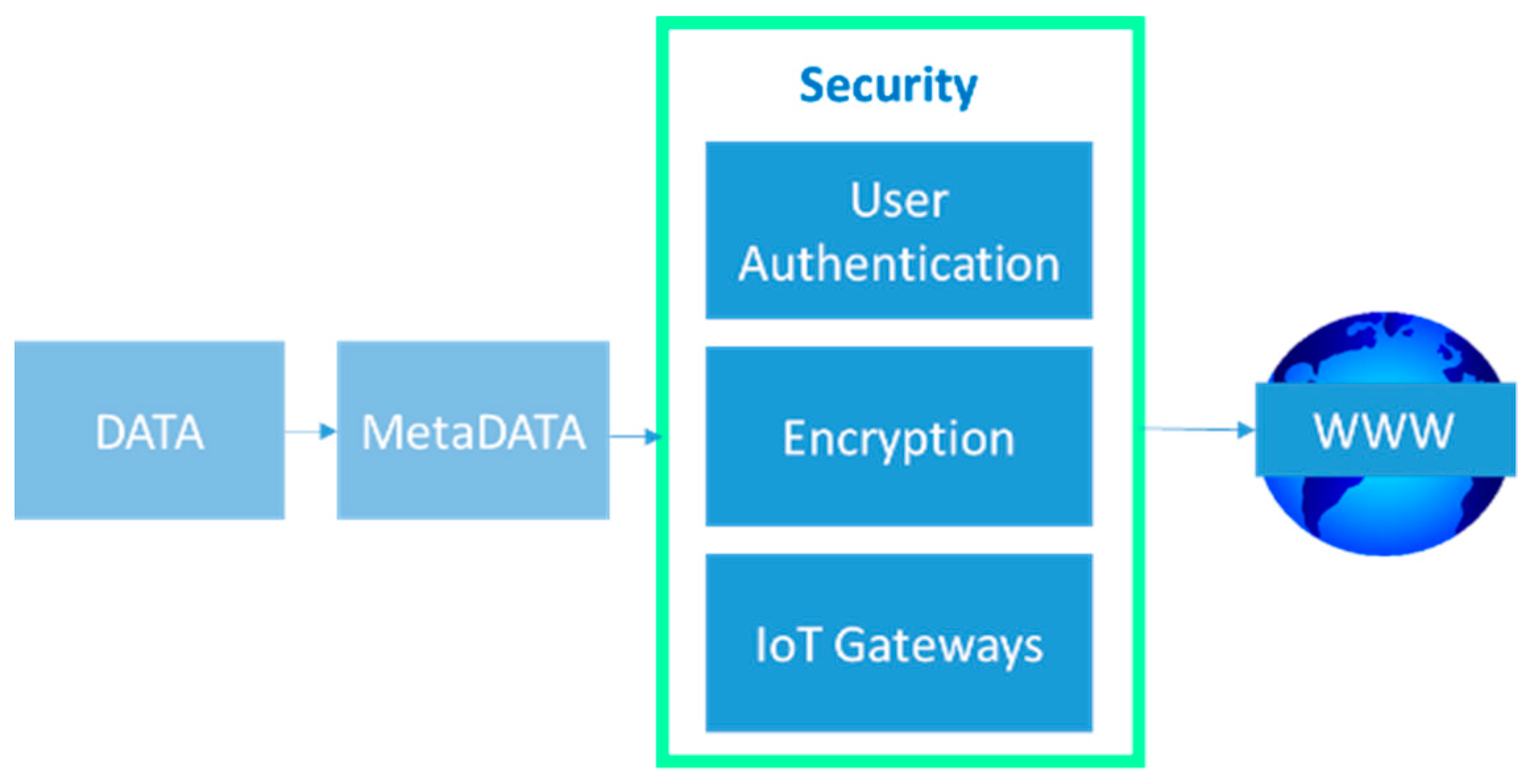
As such, after establishing the basic security layer, it is recommended that third-party information security solutions be employed to address the different safety aspects of the data, as listed in Figure 3.

2.4. Layer 4: Service Layer

The topmost layer of the proposed architecture is the service layer. The traditional functions of the service layer are retained in the IIoT architecture. The service layer can act as the platform that establishes connectivity to remote devices and services. With the advent of cloud computing services, it is apparent that data analyses can be cost-effectively performed using cloud services. The service layer can be used to interface with such cloud computing services and, depending on the level of confidentiality, a dedicated data transfer medium or a general medium can be selected. Many industries will have numerous suppliers and vendors and the service layer can be used to interact with these parties. This capability reduces miscommunication and also adopts a proactive approach to engage supplier services.

3. The Cloud Computing Role in the IoT

Once the architectural design of the IoT application is determined, the second important part in the IoT application is the design of the cloud computing role. In the IoT applications, the size of the project has to be planned out as early as possible. This is because most developers would scale the size of the application up once its early implementation is successful. The scaling itself will be a challenge if it is not planned earlier. This would lead to redundant work if the scaling capability was not included in the developed application. This section of the paper serves as a guideline to identify which path to take for one’s application with respect to cloud computing services.

3.1. IaaS, PaaS, or SaaS

Cloud computing services have three different categories based on their requirements, namely, the Infrastructure as a Service (IaaS), the Platform as a Service (PaaS) and the Software as a Service (SaaS). The IaaS provides an infrastructure that consists of computer resources and servers with network connectivity and cloud capability. Users have direct access to their servers and storage, usually via an Application Programming Interface (API). The PaaS is built on a physical server infrastructure and it provides a platform on which users can build their own software. Meanwhile, SaaS provides ready-to-use software that can be accessed remotely by the users as long as there is an internet connection. A few SaaS examples are Google Apps, Microsoft Office 365, or Adobe Creative Cloud.

In the development of the IoT application, we chose between IaaS or PaaS to build our software because SaaS does not provide us with the required platform for software development. The next question is determining which category we should choose, IaaS or PaaS? The selection depends on a few criteria that are described in

Table 1. The differences in criteria between the Infrastructure as a Service (IaaS) and the Platform as a Service (PaaS).

Criteria	IaaS	PaaS
Developer’s main focus	Storage, networking, computing	Building application
Platform flexibility to build software	Flexible as the developer build the software on a platform that is on a common infrastructure	Non-flexible as the developer build the software on a platform specific to the provider
Learning curve	Higher learning curve as the developer has to build both the platform and the software	Lower learning curve as the developer only has to focus on the software
Scalability	Allows for more flexibility	Has a certain scalability limit
Intercommunication between software	Allows for software from different platforms to communicate easily on the same infrastructure	Software from different platforms must communicate to each other from different infrastructures

.

3.2. Vendors Option, Costs, and Data Transmission Procedure

There are four big cloud computing service providers available at the moment that dominate the current cloud computing service market, namely, Amazon Web Services (AWS), Microsoft Azure, Google, and IBM. Depending on the users’ requirements, it is best to research each vendor based on their advantages and disadvantages.

The cost varies from vendor to vendor. Some of them are based on usage time (per second, per month, per year, on-demand) and some, by the amount of data used. The main point is that one has to know how much data is generated on one’s application and when this data will be generated. Knowing these two factors would allow one to be able to save on the costs immensely rather than over-compensating.

The data transmission procedure mainly allows one to send in data by https, VPN, or a direct connection. From these, direct connections are the most secure but will be the most expensive. Different vendors would be able to provide different types of connection.

4. The Application of AWS Machine Learning (AML) for the Surface Finishing Process

This section illustrates the example of an application of AML for the prediction of chamfer length as a result of a surface finishing process. The monitoring of the surface finishing processes in the aerospace manufacturing industry has become one of the key issues in maintaining the overall quality of the products or parts. To date, the surface quality monitoring post-machining processes, such as deburring and polishing, rely on visual inspections, surface roughness tests, and ultrasonic and laser gap gun measurements, which require a considerable amount of time and a skilled operator. This process-monitoring aims to eliminate the surface anomalies by halting production when defects (or part size deviations) are detected. In addition, the early detection of part size deviations will also reduce the production cost and increase the efficiency of the manufacturing processes.

4.1. Research Motivation, Experimental Setup, and Data Acquisition

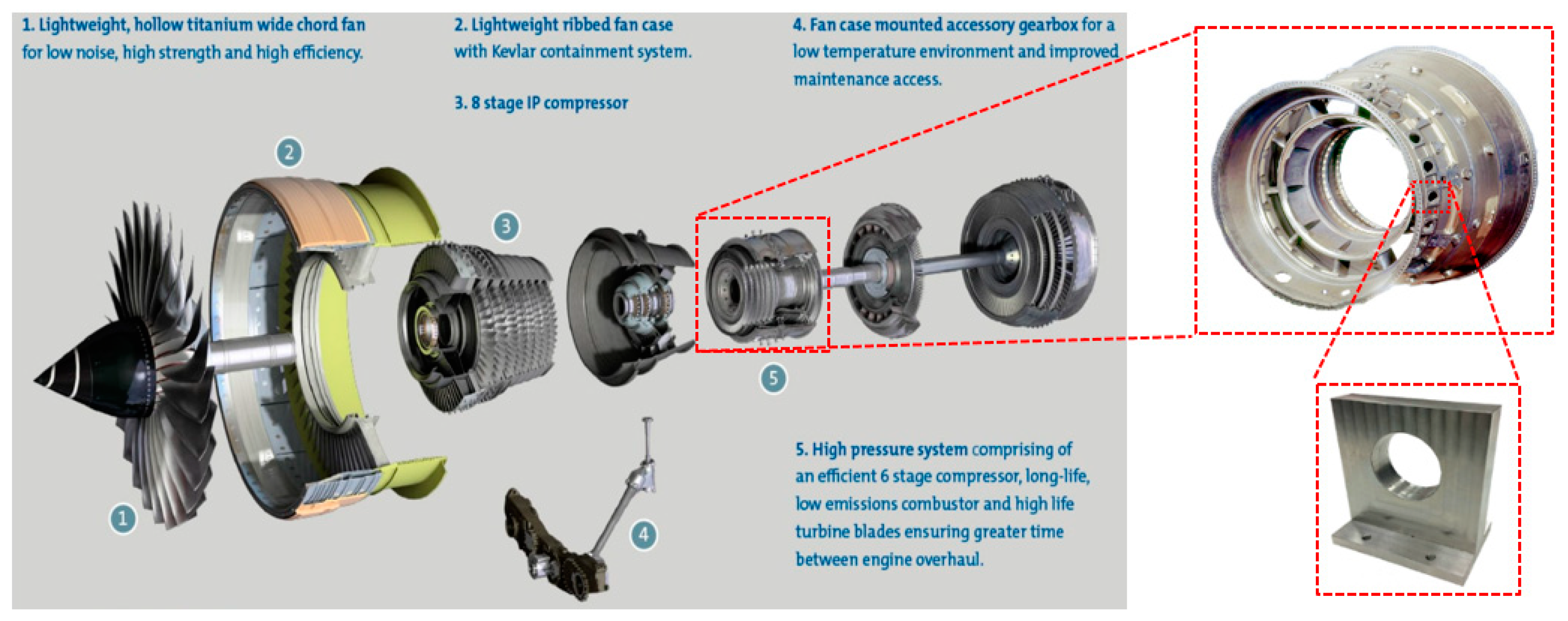
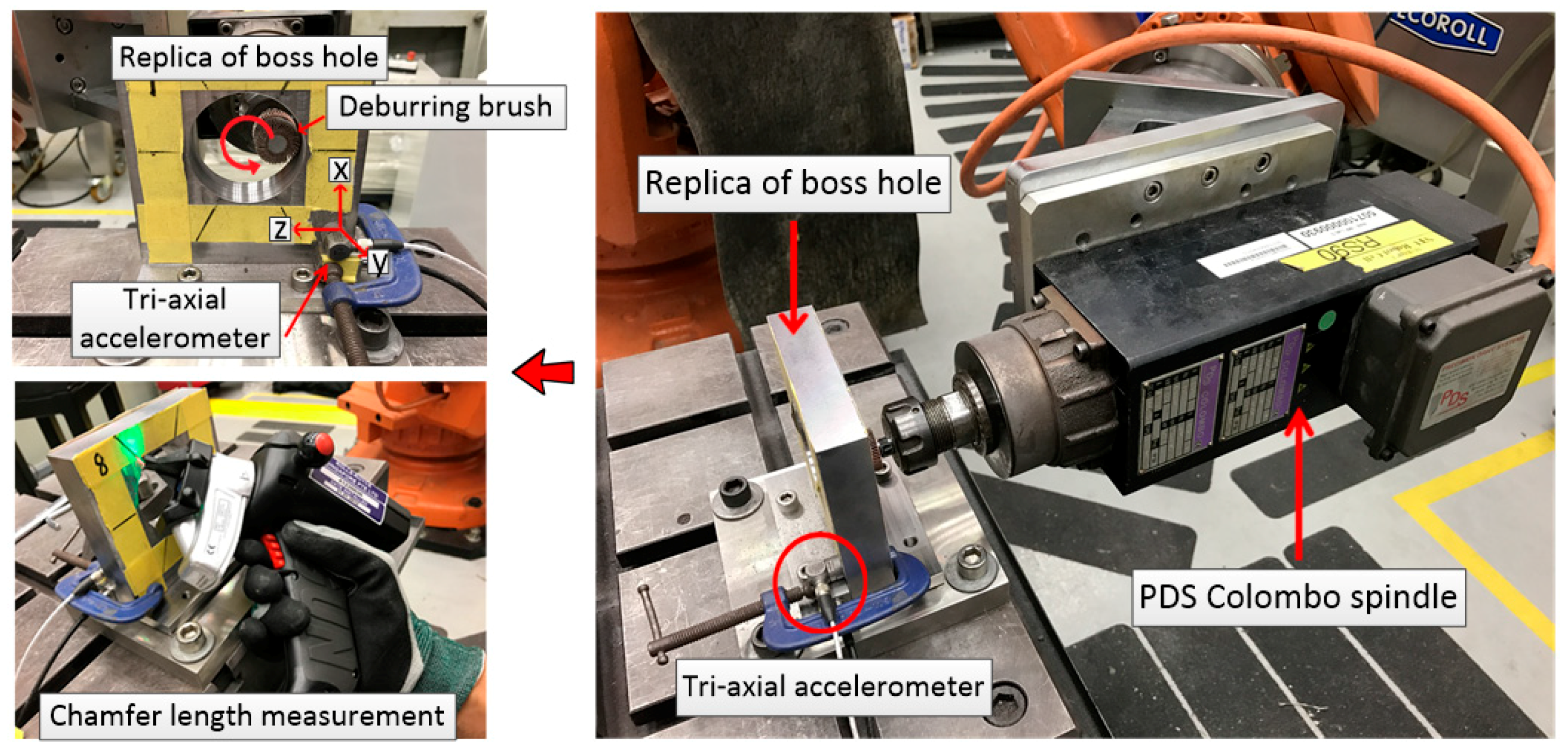
Deburring in aerospace manufacturing processes is a treatment for removing burrs, sharp edges, and rough surfaces. The importance of deburring is growing as the product quality tolerance becomes tighter and high-precision devices become the norm [10]. The deburring process is important for the safety of the critical components of the aircraft engine, as well as for eliminating stress concentration. In this paper, the deburring process being analysed is the one that is applied on the boss holes of the combustor case in aircraft engines to remove any burrs and to chamfer the hole edges (see Figure 4). For an assembly process, the precision of the boss-hole diameter and chamfer is essential. The surface quality parameter is, therefore, the chamfer length of the boss-hole edges. To date, the chamfer length measurement is carried out by a direct measurement conducted by a skilled operator. However, this dependency might lead to product quality variations. In addition, a direct measurement requires a considerable amount of time as the measurement process needs to interrupt the production cycle. For the measurement, the combustor case needs to be detached from the fixture. When the chamfer length of the component does not meet the requirements, it needs to undergo an identical process again. As aerospace industries are looking for a process that would drive down the manufacturing time, they recognized that an in-process sensing solution is a potential tool to overcome the issue. One thing that should be highlighted is that in-process sensing requires a machine learning method to be implemented. A preliminary study on the offline machine learning method has been presented in Reference [11].

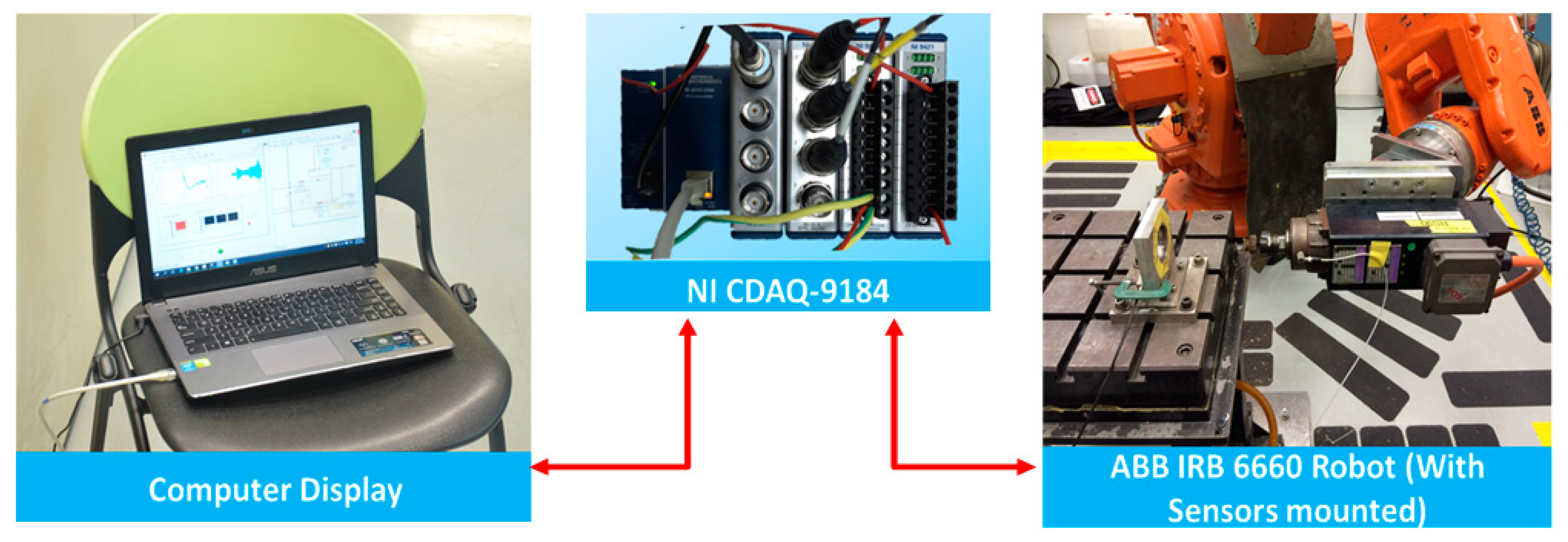
To answer the aforementioned challenge, an experimental setup to represent the actual process on the shop floor is established. The experimental setup requires the preparation of a work coupon, ABB robotic programming, and a vibration data acquisition system, including the use of an accelerometer and LabVIEW (2015, National Instruments, Austin, TX, USA). The work coupon was designed to replicate the combustor casing boss hole, as presented in Figure 4. It was designed to represent the actual Trent 700 combustor casing boss hole during the lab-scale deburring process. A detailed specification of the work coupon can be found in Reference [11]. The deburring experimental setup is shown in Figure 5 and Figure 6. It comprises an ABB IRB 6660 robot with an electric power spindle (PDS Colombo RS 90). A standard mounted flap wheel (aluminium oxide) with a grit size of P80 is used as the deburring brush for removing the burrs and sharp edges of the boss-hole replica. The rotational speed of the spindle is controlled by a variable frequency drive set to 166.67 Hz, which corresponds to 10,000 RPM and a feed rate of 30 mm/s.

The 3-axis accelerometer was attached to the work coupon as shown in Figure 6. The accelerometer used in this study is a Kistler 8763B IEPE (2016, Kistler, Winterthur, Switzerland) accelerometer with a sampling frequency of 40 kHz. The NI 9234 module from National Instruments with a maximum sampling frequency of 51.2 MS/s is utilized to record the signal. The data acquisition was performed using an NI-DAQ 9184 chassis, coupled with a supporting module for the respective sensor.

The data acquisition was run synchronously with the robot spindle movement. The vibration signal was triggered as soon as the abrasive tool was in contact with the work coupon and it automatically stopped when the tool completed one cycle. The vibration data were then saved onto the PC once one cycle of the deburring process was completed. The chamfer length was also measured after each cycle of the deburring process was completed. The aim of measuring the chamfer length was to use this data in the learning process of the machine learning method. The chamfer length measurement process using the gap gun is shown in Figure 6.

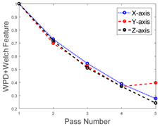
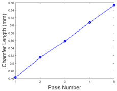
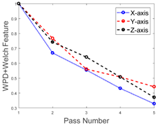
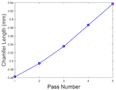
In this study, one complete cycle of the deburring process on one side of the work coupon (replica boss hole) is referred to as one “pass”. During one pass, three sets of vibration signals are generated from the X, Y, and Z directions of the 3-axis accelerometer. A detailed visualization of the three directions can be seen in Figure 6. To remove the burrs that are produced from the previous manufacturing process and to develop a chamfer on the boss-hole edges, five passes of the deburring process and data acquisition are conducted. A more detailed visualisation of the vibration signals obtained from the deburring process is presented in Reference [11]. A feature from the combined wavelet decomposition and Welch’s spectrum estimation is calculated and applied to obtain the raw vibration signal. This feature is selected based on a previous study [12]. The feature extraction results of each pass and the associated chamfer length for each pass are presented in

Table 2. The vibration features of the three axes for the training data.

Pass No.	Accelerometer Axis			Chamfer Length (mm)
	X	Y	Z
1	1	1	1	0.462
2	0.729	0.698	0.717	0.515
3	0.544	0.522	0.510	0.558
4	0.388	0.369	0.369	0.607
5	0.277	0.396	0.242	0.653

and

Table 3. The vibration features of the three axes for the testing data.

Pass No.	Accelerometer Axis			Chamfer Length (mm)
	X	Y	Z
1	1	1	1	0.462
2	0.669	0.767	0.742	0.494
3	0.554	0.560	0.641	0.535
4	0.431	0.508	0.507	0.586
5	0.328	0.442	0.371	0.637

.

Six work coupons were used in the experiment. Three were used for the machine learning training process and the remaining three were used for testing the process. For demo simplification of the AML prediction, we calculated the mean value of the features and the associated chamfer length from the three work coupons for both the training and testing processes. We then normalize the feature into the form of the baseline. The objective was to obtain a better visualisation of the decreasing trend of the feature values associated with the increasing number of passes. It can be seen from Table 2 and Table 3 that the decrease on the features (X-, Y-, and Z-axis) corresponds to the increasing number of passes and the chamfer length.

4.2. Amazon Web Services Machine Learning (AML)—General Overview

In this paper, the AML functionalities and APIs for the chamfer length prediction in the deburring process are presented. Prior to the AML platform application, the vibration features of the deburring process must be predetermined. The measured chamfer length is also needed as the target prediction of the training process in order to build the prediction model. The detail of the developed feature based on WPD and Welch is presented in our previous study [11]. The AWS client provides APIs for users to build and to evaluate the machine learning models. Once we have designed a model that is capable of chamfer length predictions, we will build an infrastructure to communicate between the AML and the chamfer length prediction application in a dynamic chart. The infrastructure will consist of a webpage, a server, sensors, and the machine learning application. The Javascript and PHP scripts will be used to automate the process of sending the new data to the server, communicating with the AML client to request for the predictions, storing the prediction data, and presenting the predictions on the webpage.

The first part of our problem is confirming if the machine learning model created by the AML client is able to predict the target output at within a certain degree of accuracy. Using the selected feature, we will create a machine learning model and utilize the service functionality on the AWS to evaluate its performance. After some assessments, we will determine whether the features have a linear correlation to the target output.

The second part of our problem is integrating the AML into our database and webpage in order to achieve real-time data visualization. We will first create an application to work with the AML client in order to generate predictions from the machine learning model. We will make use of the SDK provided by the AWS to call upon a real-time prediction end-point based on the AWS APIs and output the predictions into our database. Next, we will connect the database to our webpage and create a script to automatically update the chart with prediction data in real-time.

The objective of this study is to develop an indirect real-time monitoring system equipped with machine learning capabilities to predict the chamfer thickness during a deburring process. To achieve this, the project is segmented into the following tasks:

• Understanding the AML functionalities
• Vibration feature selection for the deburring process
• Building the machine learning model
• Building the machine learning prediction application
• Webpage design for data visualization
• Database creation for data storage and access
• Integrating the machine learning application, database, and the designed webpage
• System testing

4.3. Amazon Web Services Machine Learning (AML)—Algorithm Perspective

Machine learning on the AWS is classified into three main categories, i.e., (1) the machine learning application service, (2) the machine learning platform service, and (3) deep learning on AWS. The machine learning application service consists of APIs for vision services, language services, and chatbots. Some use cases include face recognition services, speed recognition, speech-to-text translations, and the building of interactive chatbots. Deep learning on AWS is dedicated to the development of artificial neural networks. In this paper, the machine learning platform service will be explored and applied to obtain the deburring data. In the second class, the AWS Machine Learning (AML) platform is essentially a Software as a Service (SaaS) solution developed by Amazon with the ability to work closely with other AWS functions in order to create machine learning models which can subsequently be utilised to fetch the required predictions. Users can choose from real-time predictions and batch predictions based on the size of the datasets.

Although the full details on AML implementations are not publicly available, the service documentation and API are able to provide sufficient information on its functionality. These detail that the machine learning performed on the service is based on the linear regression and logistic regression algorithms. Both algorithms are less complicated than other machine learning-based regression methods, e.g., artificial neural methods (ANN) and support vector regression (SVR) methods. However, these algorithms are suitable for binary, classification, and regression machine learning problems in industries with less complex datasets.

In addition, AML uses two types of algorithms—e.g., (1) the linear regression algorithm and (2) the logistic regression algorithm—to produce three types of machine learning models. The linear regression algorithm consists of squared loss functions, where the stochastic gradient descent is used for the logistic regression models. These are basic standard algorithms and are able to be efficiently applied to machine learning problems in the industry [13]. Binary classification models utilise the logistic regression algorithm which consists of a logistic loss function and a stochastic gradient descent. Multiclass classification models utilize the multinomial logistic regression algorithm which consists of a multinomial logistic loss function and a stochastic gradient descent.

These models are selected depending on the problem that the user is looking to solve. If the user wants to predict an output value from a set of input values, the linear regression model should be used. On the other hand, if the user seeks to classify the inputs values into two outcomes/categories, the binary classification model should be used. If the user is looking to classify the inputs into a range of outcomes/categories, the multiclass classification model should be chosen.

4.4. Amazon Web Services Machine Learning—An Example Deburring Data Application

4.4.1. Prediction System Architecture

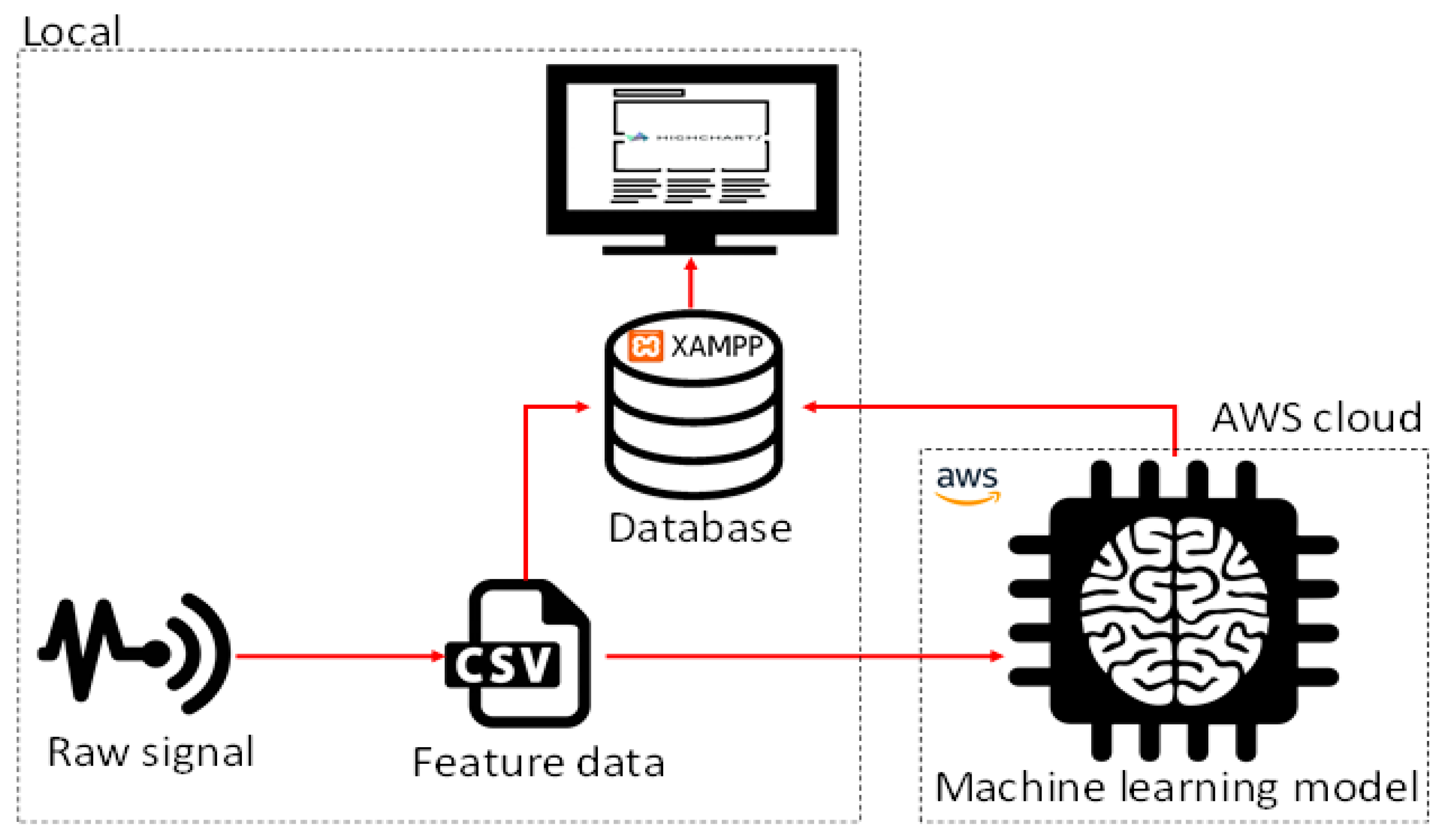
In our approach, most of the components of our system will run locally except for the real-time prediction of the machine learning model which will run on the AWS cloud. The local components include the sensor signals, the feature data, the database, and the data visualization chart. Figure 7 shows a pictorial representation of our monitoring system.

4.4.2. Developing the Machine Learning Model on AML

There are two processes involved in the development of a machine learning model on AML: (1) the training process and (2) the testing/evaluation process. In the training process, users need to specify the following:

• The input training data source
• The data attribute that contains the target variable
• The data transformation instructions (recipe)
• The training parameters required to control the learning algorithm

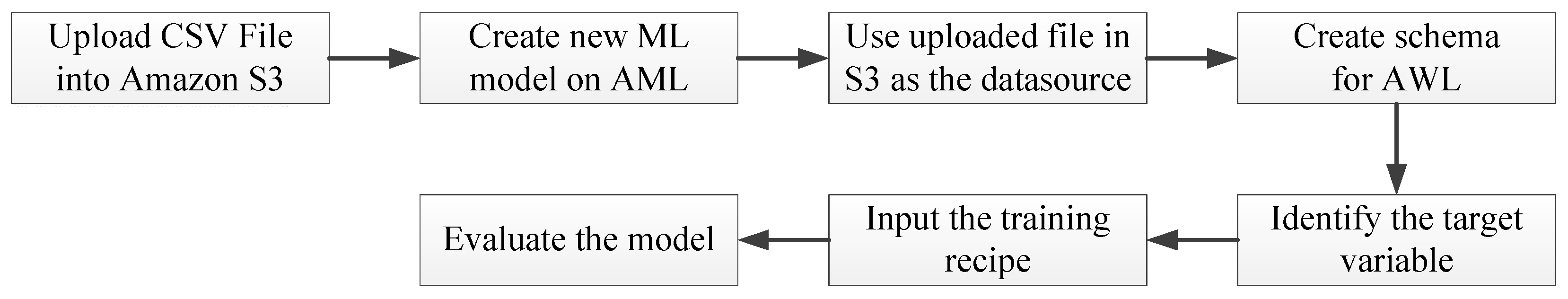
To start the evaluation process on AML, we require a machine learning model that will be created after the training process. A data source with a scheme similar to that of the training data source must be created before it proceeds to the evaluation. The actual values of the target variable must also be included in the evaluation data source, as AML will compare the actual values with the predicted ones. The general process flow for developing a machine learning model on AML is illustrated in Figure 8.

Since our aims are to predict the chamfer length based on the features extracted from the three axes of the (X, Y, and Z) vibration signal, a multivariate linear regression is used. It is worth noting that the inputs and output must have a linear relationship for the model to perform effectively. This requirement has been tested for the features and the chamfer length. The full data used for creating the machine learning model are presented in Table 2 and Table 3. We used 50% of the dataset to train the model and the other 50% to test and evaluate the model. By utilising the framework provided by AML, a regression model was created and evaluated. Two CSV files, one containing the training data and one containing the testing data, were first uploaded onto Amazon S3, which is a cloud-based database developed by AWS. The motivation for using this database was due to the ease through which the data could be access by AML. Following this, we used the AML interface to create an input data source pointing to the training CSV file. The interface automatically assigns a datatype based on the values in the CSV file. The datatype will be assigned as binary, categorical, numeric, or text. Users can change the datatype accordingly if the assigned datatype was incorrect. For our dataset, we assign the numeric datatype to the chamfer length and to the corresponding X-axis, Y-axis, and Z-axis power spectrum density magnitude values. The pass is assigned as a categorical datatype.

Subsequently, the interface will request the user to select the target variable. Based on the datatype of the selected target variable, the interface will decide on the type of algorithm to use to train the model. If a numeric datatype was selected, the linear regression algorithm is used; if a categorical datatype was selected, the multinomial logistic regression algorithm is used; and if a binary datatype was selected, the logistic regression algorithm is used.

Table 4. The Amazon Web Services Machine Learning (AML) machine model selection based on the target variable datatype.

Target Variable Datatype	Machine Learning Model
Binary	Logistic regression
Categorical	Multinomial logistic regression
Numeric	Linear regression

gives the associations between the machine learning models and the target variable datatypes.

In our case, as the target variable—i.e., the chamfer length—is a numeric datatype, the AML client automatically assigns the linear regression algorithm for the model. The AML client allows users to use the default recipe or to code their own recipe, which sets the parameters for the machine learning training process. The default recipe provided by AML will split the data source in two, 70% of the data source being used for the training set and the remaining 30% being used to evaluate the machine learning model performance, as shown in Figure 9.

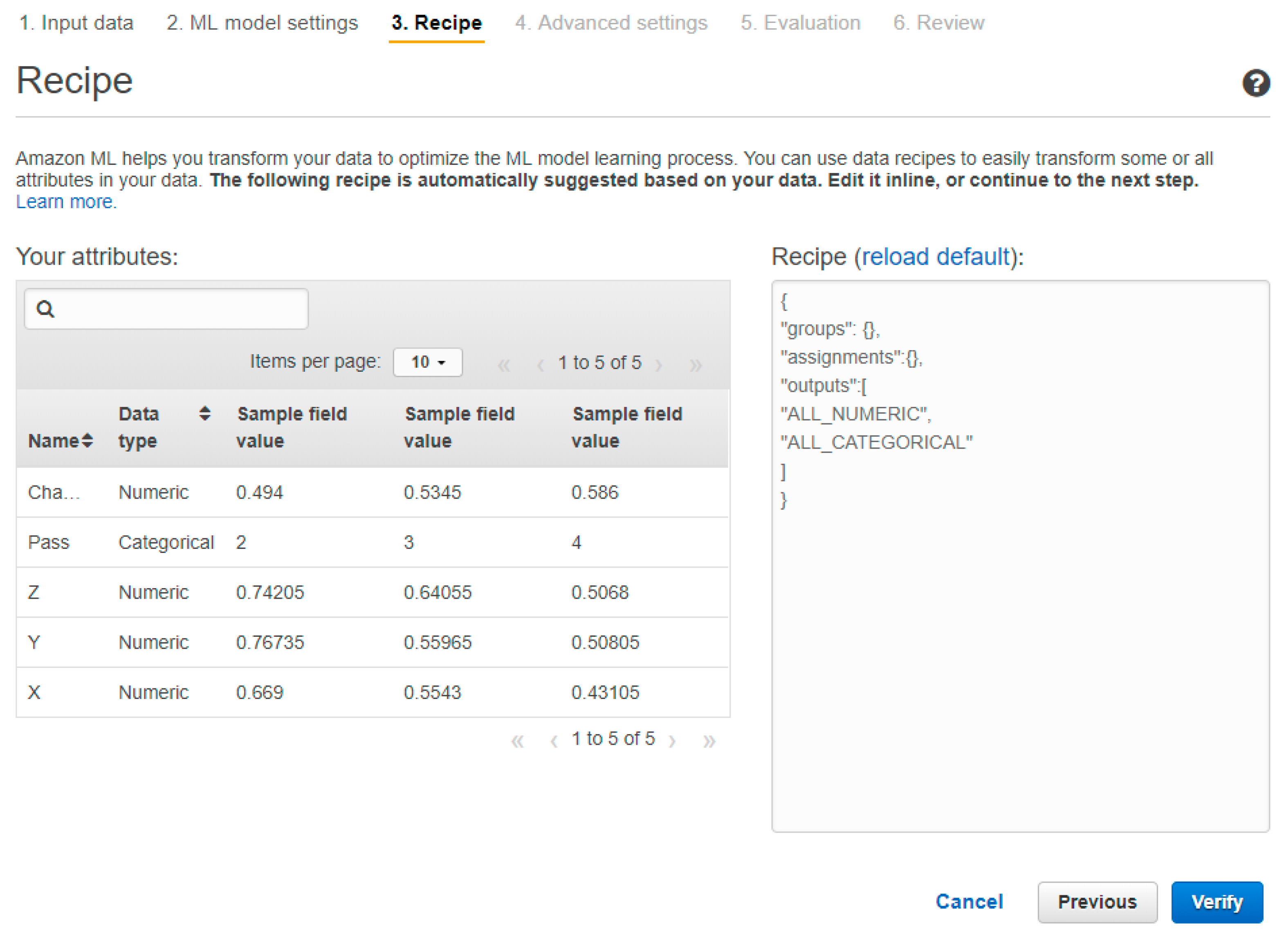
On the other hand, AML provides a custom recipe option for users to code in a specific syntax. The custom recipe allows users to decide on the training parameters for the machine learning model, to apply data transformation tools provide by the AML APIs, and to decide how the data source will be split to train and evaluate the machine learning model. The custom recipe must contain the following 3 sections:

• Groups: to group various variables. This allows for the data transformations to be applied more efficiently.
• Assignments: to create intermediate variables that can be reused.
• Outputs: to define the variables to be used in the training process and to apply the data transformations where required.

All the data in our data source will be used to train the machine learning model. Thus, we do not need to apply any groupings or data transformation. Hence, we applied a custom recipe to train our machine learning model based on these specifications, as shown in Figure 10.

After creating the machine learning model, we used the evaluation function to create a new data source that pointed to the testing CSV file in S3 and proceeded to evaluate the machine learning model. The evaluation results will be discussed in Section 4.4.7.

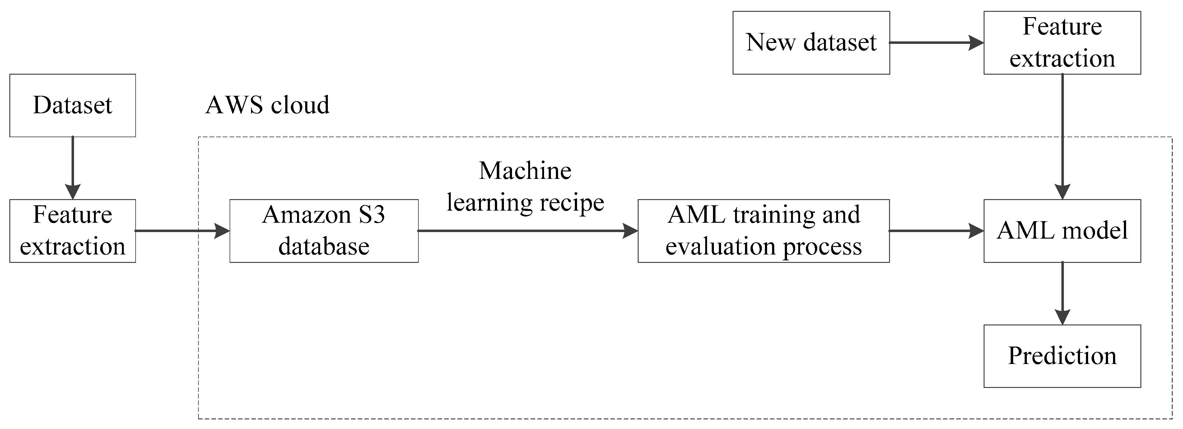
With the machine learning model created and evaluated, we can subsequently proceed to generate predictions using the model. Figure 11 provides an overview of the model creation process on AML and how it will be used to create predictions.

4.4.3. Webpage Development

For a monitoring system to be available to broadcast information, a webpage needs to be created and hosted on the World Wide Web (WWW). This will allow users to monitor the progress of the process at any point in time as long as they have an internet connection. Additionally, security features can be added to the webpage to maintain the confidentiality of the information displayed when required.

HTML is used to create the webpage. The HTML code consists of a header to display the title of the page and a body, which will hold the chart for the data visualisation. Additionally, it requests the required libraries to produce a dynamic chart.

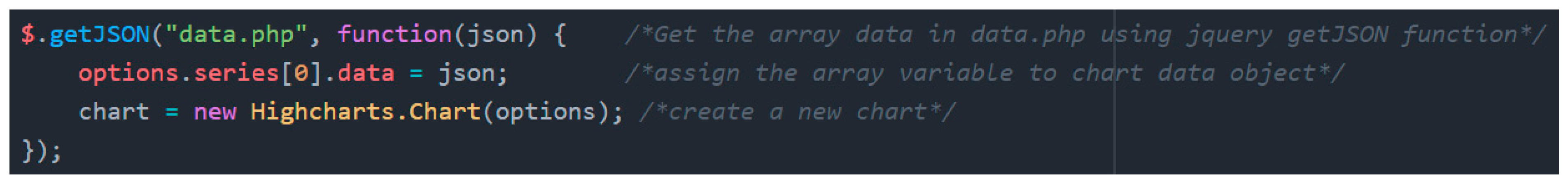
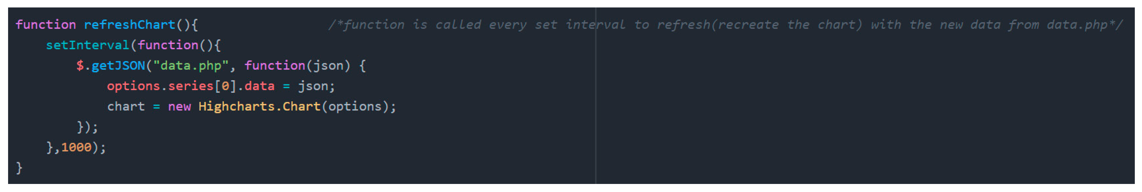
To create the data visualisation chart, a javascript library known as Highcharts was utilized. Highcharts was chosen for to several reasons. Firstly, it is a generic library that allows for the simple integration with major web frameworks. Additionally, it is based on a scalable vector graphics technology and works with HTML5, which is the current trend in data visualization [12]. The HighCharts library is able to create dynamic charts which allow users to interact with the data. It is also an extremely flexible library with a wide range of charts to choose from. This is important in order to create impactful charts that are able to convey the trends and focal points clearly. Since the aim is to create a real-time system, the chart needs to be able to refresh itself whenever new data is obtained. To achieve this, the refreshchart function is called upon from the HighCharts library and the chart is set to refresh every 5 s. This timing was obtained by taking into account the average time required for each pass in the chamfer deburring process. The chart refresh function in HTML is presented in Figure 12.

4.4.4. Creating the Database

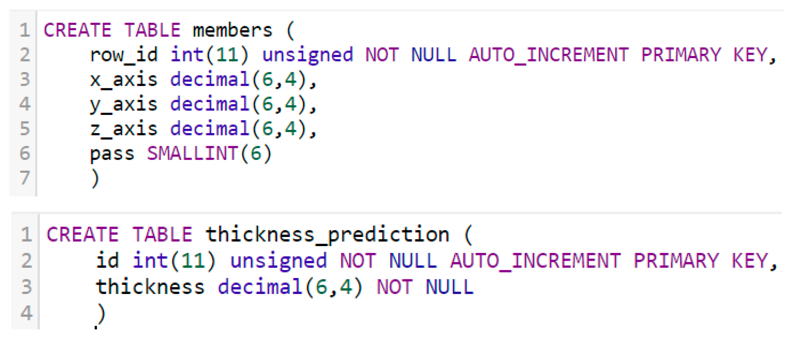
To better simulate the actual manufacturing shop floor and provide a mean for data access and storage, we created a local server. The server stores the sensor data, stores the prediction data, and enables the webpage to retrieve and display the required data. For this project, we will be utilising XAMPP, a free cross-platform web server solution which includes MySQL and PHP interpreters. MySQL is an open-source relational database management system which will be used to store our datasets and PHP will be used for developing server-side scripts. Additionally, XAMP also provides a Graphical User Interface (GUI) for MySQL, which simplifies the database creation process.

The database will consist of 2 tables, one for storing the sensor data and the other for storing the prediction results. To create the tables, we initiated the queries shown in Figure 13.

4.4.5. Connecting the Webpage to the Database

To bring in the datasets into the javascript file and to produce the charts, the javascript file must connect to the server and fetch the required data. This is carried out through PHP programming. PHP is a popular server scripting language which was designed for web development. Hence, the PHP code communicates with the server and returns the required datasets. Since the chart is generated by a javascript file, we require a section of code in javascript to call the PHP code to update the datasets. This is detailed in Figure 14.

For this process to work effectively, the PHP code needs to establish a connection to the MySQL database, query the database for the prediction data, and output the data according to the syntax required for HighCharts.

4.4.6. Building the Real-Time Prediction Application and Scripting Data Import

The AML client provides two ways to generate the predictions using the machine learning models, i.e., (1) batch predictions and (2) real-time predictions. Batch predictions are useful if users have a large dataset that they want to predictions to at once. We will utilise real-time predictions for this project as we want to predict the chamfer length in real-time after every pass and thus, our dataset is small.

Initiating real-time predictions on AML will create a real-time endpoint and an endpoint URL is produced. This will allow users to call upon the real-time prediction API to generate predictions. Since the client does not provide an interface to work with the API, we will create an application to create a prediction request from our CSV file and direct the output to our server. This will allow us to display the real-time predictions on our system subsequently.

Using the SDK provided by AWS, we created a python script which established a connection to our AWS account and retrieved the machine learning model we created in Section 4.4.2, along with the prediction endpoint. The script then opens the CSV file that contains our sensor data, converts the CSV format into a string type, and calls the machine learning API to predict the chamfer thickness. Following which, the script stores the predicted value into the table in the MySQL database that we created in Section 4.4.1 and rename the CSV file to include the current date and time for archiving.

4.4.7. Prediction System Result and Analysis

The developed system was successful in generating predictions using the python application, importing the output into the local MySQL database, and displaying the predicted chamfer length on a dynamic chart.

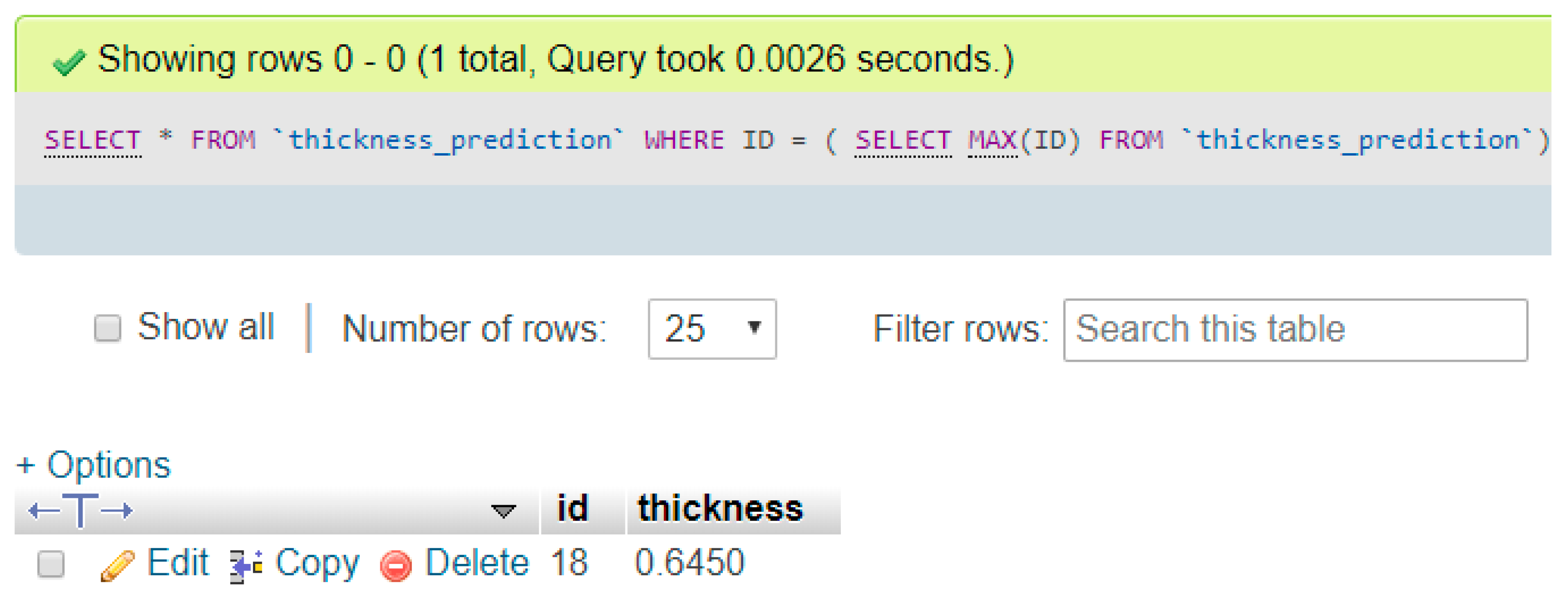
When conducting the system testing, the python application displayed the prediction result and imported the sensor data and predicted data into the local database, as shown in Figure 15. Additionally, we confirmed that the prediction result was successfully written into the database by querying the latest input, as shown in Figure 16.

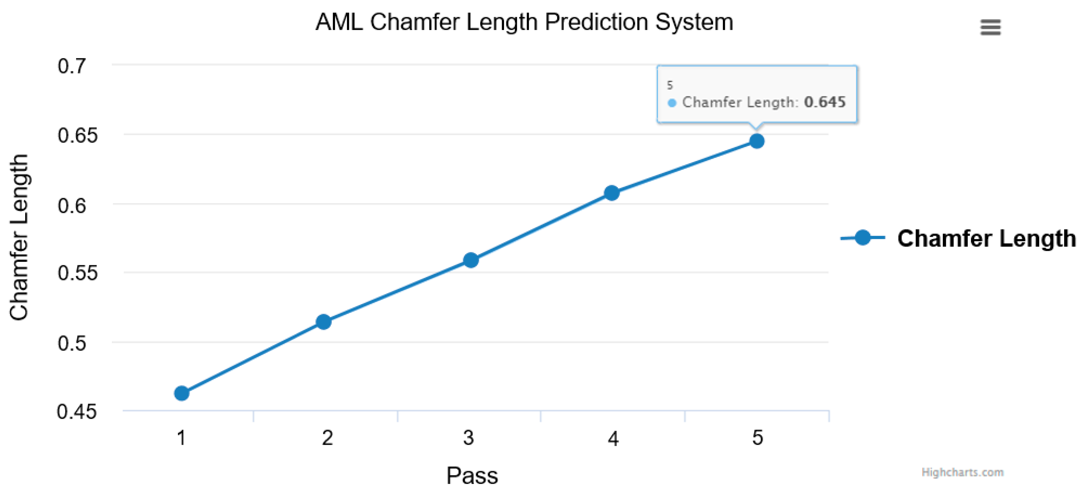
Finally, we confirmed that the chart updated the predicted the chamfer length when we accessed the webpage, as shown in Figure 17.

Evaluation is performed on the machine learning models by means of supervised learning to determine their reliability when new data are introduced. As future target values are unavailable, model evaluation is carried out using the testing dataset that we previously split from our data source. Additionally, an accuracy metric is required to assess the model’s performance. It is important that the testing dataset used is different from the dataset used to train the model as the hypothesis is created from the training data. By doing so, we will obtain a reliable prediction result only if we evaluate the model with a different dataset.

The AML client has various metrics for measuring the machine learning model accuracy depending on the type of the created model. We will focus on the metric used for the regression models as it is the model used for this project. AML uses the root mean square error (RMSE) metric to measure the accuracy of the regression models. This measurement is an industry standard and it is based on the difference between the model’s output variable and the actual target output.

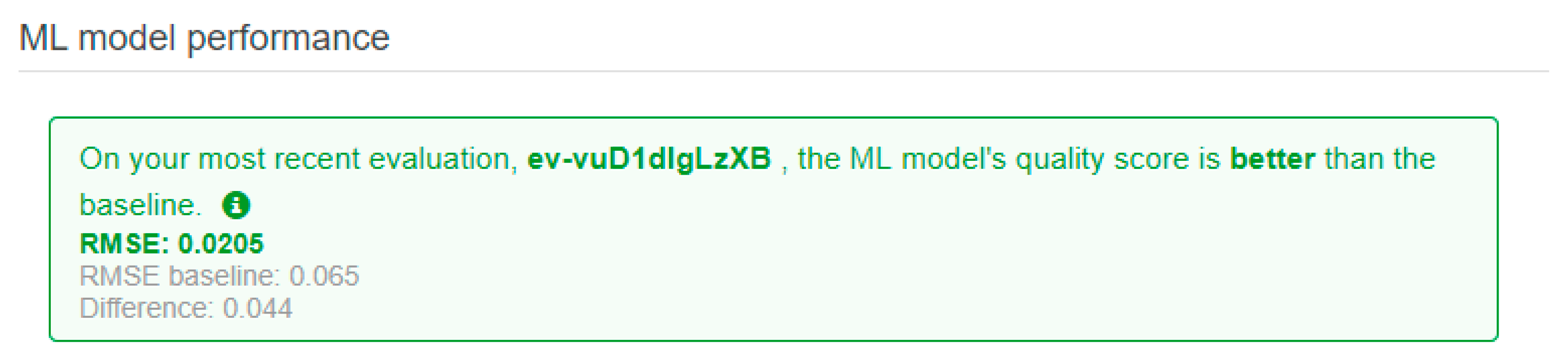
A smaller RMSE value would translate to the model having a better predictive accuracy, with a perfect model having an RMSE value of 0. The AML client provides a baseline metric for validating the regression models. This baseline is attained by assuming that the actual output is the average target value predicted by the regression model. Hence, for this report, we will use the baseline metric to ascertain if the machine learning model is suitable for predicting the chamfer thickness. By using the AML client to evaluate the model, we achieved a desirable model performance which has a better performance than the baseline. The RMSE score is shown in Figure 18.

We observed that the RMSE value of the testing data is 0.0205 and that it is lower than the baseline value of 0.065. This means that the model is able to predict the chamfer length more accurately than a model that always predicts the mean value of the actual chamfer length provided in the training data. From this, we can deduce that the model is satisfactorily accurate in predicting the chamfer length of the testing data. 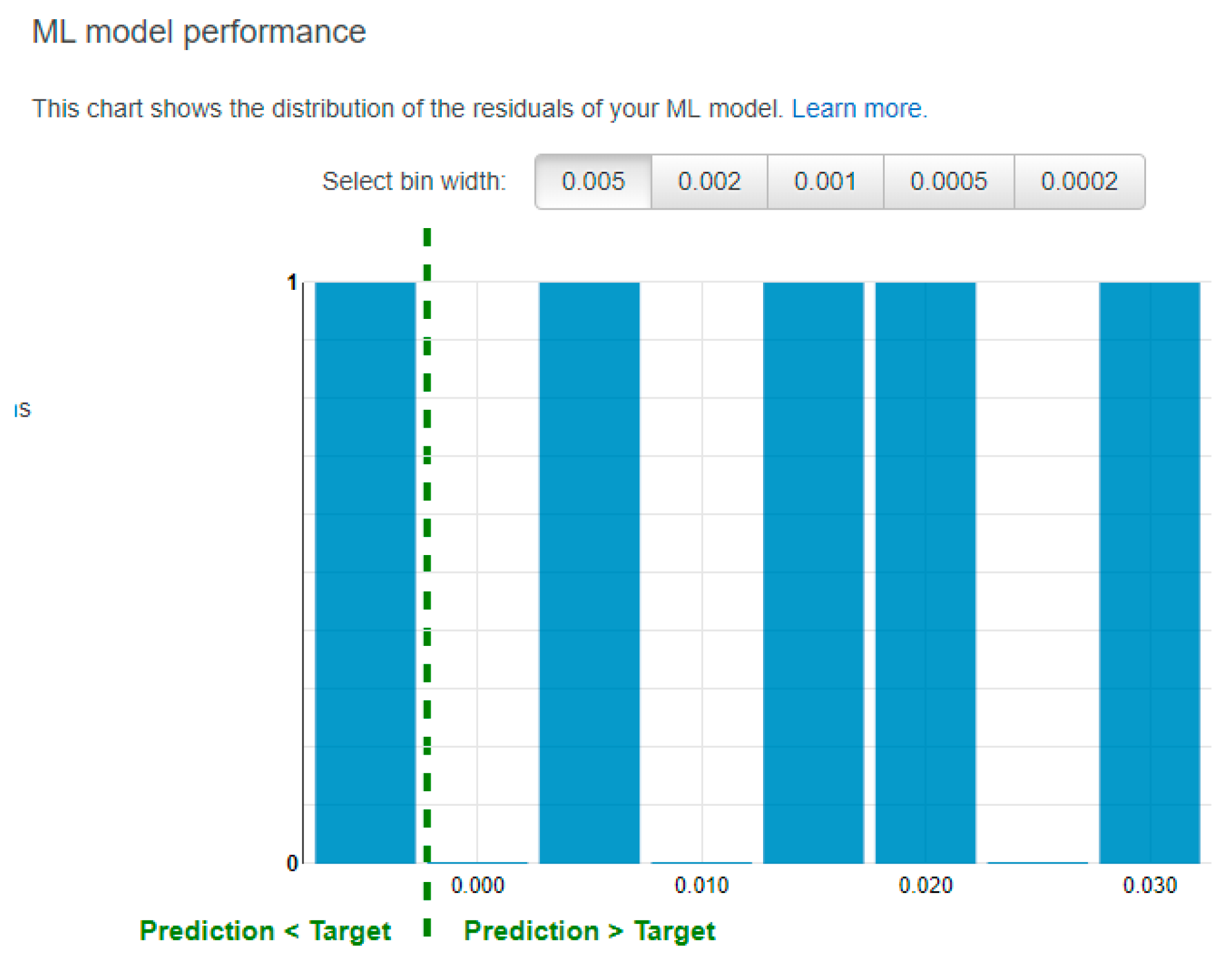Figure 19 shows the distribution of the residuals in the ML model. The residual values refer to the difference between the actual output and the predicted output. Hence, a positive residual value implies that the model is underestimating its predictions and a negative residual value suggests that the model is overestimating its predictions.

By looking at the residual chart presented in Figure 19, we observe that the machine learning model generally underestimates the chamfer length because 4 out of 5 predictions made in the evaluation are less than the actual output. Nonetheless, the predictions are quite accurate, with an RMSE of 0.0205. However, it is important to note that due to the small training and evaluation data sizes, although the results reveal a positive model performance above the baseline, the model may not have accurately captured the trend in the features and the target output.

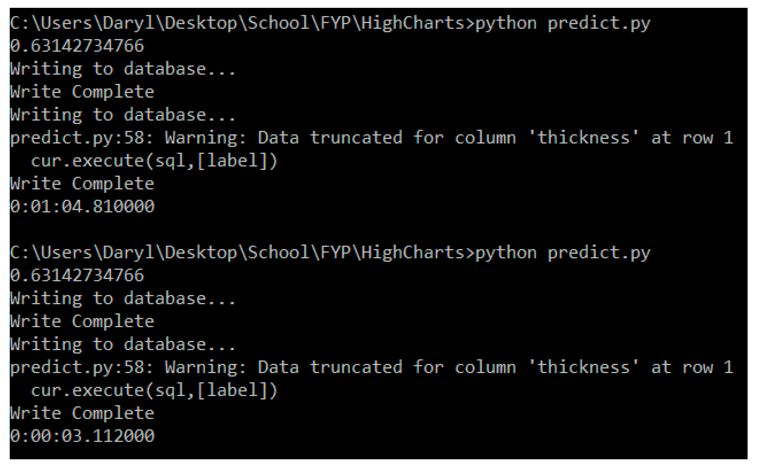
For the developed system to perform better than the current standards, we need to look at the speed of the system by determining how long it takes to predict the chamfer thickness upon receiving the sensor input. This is achieved by introducing the following lines of code into our python script:

• From datetime import datetime
• startTime = datetime.now()
• #Python Script to generate predictions and archive data
• Print datetime.now()—startTime

From this, we observed that the script takes longer to run the first prediction (approximately 1 min), but that that timing decreases to approximately 5 s in the subsequent runs. This is exemplified in Figure 20.

Hence, we can see that utilizing this system of indirect real-time predictions, as opposed to the current direct method, allows us to avoid the time required to remove the component and measure it. This translates to significant time savings. However, it is also noted that this is highly dependent on the accuracy of the machine learning model. Incorrect predictions could lead to greater inefficiencies, especially when high tolerance levels for the process are observed.

5. Conclusions

A brief review of the IIoT applications, architecture design, and cloud computing has been presented. The review is followed by the preliminary application of AML for the indirect monitoring of the surface finishing process. The scope of the research work is the chamfer length prediction of a boss-hole replica in the deburring process using AWS Machine Learning (AML). Overall, our indirect monitoring system performed well in terms of the model performance and the time taken to generate the predictions. Additionally, AML was an effective solution in creating a machine learning model for our infrastructure. This results in a system that is relatively easy to set up. Additionally, this system offers a scalability for the prediction requests as the machine learning model on AML is capable of handling 200 prediction requests every second [13]. Additionally, this computing capability can be increased by the AWS team upon request. However, this method is dependent on the accuracy of the machine learning model. Hence, it is important to train and evaluate the machine learning model with large datasets to ensure the accuracy of the model before the system is implemented. The proposed approach in this report is also not limited to the aerospace deburring process, but to any processes which can utilize the regression or logistic regression algorithms provided by the AML client. From the results attained, it was observed that the algorithms have the potential to improve the efficiency of an aerospace deburring process and that this model can be extended to other processes where machine learning can be adopted.

The limitation of this approach is in the available machine learning methods in AML. Since the AML only provides logistic regression methods, an advanced machine learning method such as an artificial neural network (ANN), a support vector machine (SVM), or an adaptive neuro-fuzzy inference system (ANFIS) need to be developed and embedded in the AML platform in order to increase the prediction accuracy for more advanced applications such as the prediction of surface roughness and material removal rates. Logistic regression methods have a low performance when handling huge datasets. The development of some machine learning methods can be programmed in tensorflow.