A Stability Preserving Criterion for the Management of DC Microgrids Supplied by a Floating Bus

Abstract

Direct current (DC) distribution is one of the most important enabling technologies for the future development of microgrids, due to the ease of interfacing DC components (e.g., batteries, photovoltaic systems, and native DC loads) to the grid. In these power systems, the large use of controlled power converters suggests the need of a careful analysis of system stability, as it can be impaired in particular conditions. Indeed, in DC power systems, a destabilizing effect can arise due to the presence of inductor/capacitor (LC) filtering stages (installed for power quality requirements) and high-bandwidth controlled converters, behaving as constant power loads (CPLs). This issue is even more critical when the CPL is potentially fed only by the battery, causing the DC bus to be floating. In this context, Lyapunov theory constitutes a valuable method for studying the system stability of DC microgrids feeding CPLs. Such a theory demonstrates how the region of asymptotic stability (RAS) shrinks as the state of charge of the battery diminishes (i.e., as the bus voltage decreases). Once the accuracy of the RAS is validated by comparing it to the real basin of attraction (BA), numerically derived using continuation methods, a smart power management of the CPL can be proposed to preserve the system stability even in the presence of a low bus voltage. Indeed, a suitably designed criterion for limiting the load power can guarantee the invariance of RAS and BA for each equilibrium point. An electric vehicle was used herein as a particular DC microgrid for evaluating the performance derating given by the power limitation.

1. Introduction

Currently, direct current (DC) distribution represents the most innovative solution for islanded microgrids, both in transportation [1,2] and in land-based power systems [3,4]. Indeed, thanks to an even more widespread employment of power electronics and performing control systems, DC technology is not only capable of guaranteeing paramount advantages [5] (e.g., improved efficiency, enhanced power-flow control, and increased power availability), but it can also foster the optimal combination of generation, storage, and consumption [6]. Such a trend can be observed in the transportation industry [7,8] and in terrestrial systems [9,10], where many key factors and technologies are promoting this shift toward DC power systems, among which distributed energy resources (DERs) and energy storage systems (ESSs) are the most important. In fact, with ESSs and the great majority of DERs having a DC interface, the exploitation of this technology in some parts of the alternating current (AC) distribution system is becoming profitable. Moreover, several loads (e.g., data center, LED-based lighting systems, consumer electronics, etc.) are natively in DC, thus simplifying the transition. For characterizing the context in which this study is developed, a typical DC microgrid consists of a DC bus to which all components are connected through either DC–DC or DC–AC power converters. Such a DC bus is interfaced to the main AC grid through an AC–DC converter, whose main task is to control the bus voltage while balancing the power flow with the AC grid. The interactions between all these converters are usually investigated to identify possible interferences in the presence of controller bandwidth overlap.

In this context, a critical eventuality studied in academia is the constant power load (CPL) behavior [11,12], which may occur when a tightly controlled power converter (modeled as a nonlinear CPL) interacts with the inductor/capacitor (LC) filter, which is installed for ensuring the power quality requirements in DC systems. Depending on LC values and CPL power, the resonance among the nonlinear load and filtering components can jeopardize the DC microgrid voltage stability. During the past few years, several control techniques were proposed for solving such an instability [13,14,15,16,17,18,19,20], whereas the impedance-based stability criteria evaluated the impact of the nonlinear destabilizing CPL [21,22,23]. A different approach is based on Lyapunov theory [24,25,26,27,28,29,30,31], which overcomes the limits of small-signal linearization by determining the sufficient region of asymptotic stability (RAS) nearby a stable operating point. Conversely, other methods (e.g., numerical continuation analysis) can provide the actual basin of attraction (BA), as described in Reference [32], i.e., the sufficient and necessary area inside which the states can move without impairing the stability of the system. The two methodologies for obtaining RAS and BA were previously compared in Reference [33], demonstrating how the Lyapunov analytical formulation is more suitable for an online implementation aimed at guaranteeing the microgrid’s stable operation.

Starting from the last conclusion, the present paper proposes a load management method for preserving system stability in critical DC power systems. The case under study is a particular islanded DC microgrid, where the floating bus is set only by the energy storage (without any active regulation) and the supplied load is a nonlinear CPL. For such a system, the direct dependency between the decrease of the battery state of charge (SoC) [34] and the shrinking of the RAS [33] suggests employing a CPL management for maintaining a proper stability margin.

The paper is organized as follows: Section 2 describes the DC microgrid topology, together with the related circuit in battery-only operation. In this section, the effect of the floating DC bus on system stability is analyzed by means of the Lyapunov theory, whose results (i.e., the RASs) are validated using a numerical continuation analysis (i.e., the BAs) and dynamic simulations. Section 3 proposes a stability-preserving criterion based on the definition of a stability index. In particular, this criterion is based on the mathematical law that describes how the CPL power depends on this index and on the DC bus voltage. This allows dynamically limiting the maximum available power in order to maintain the same stability margins, i.e., same RAS and BA, while the battery voltage decreases. The applicability of the proposed management is discussed in Section 4, where an electric vehicle is chosen as a DC microgrid example for testing the decrease in performance. Section 5 provides concluding remarks.

2. Effect of Floating DC Bus on System Stability

This section discusses the stability degradation that can possibly arise in a floating DC bus microgrid supplying a CPL. The present paper is based on a previous work [33] published by the authors about the criticality of a DC floating bus powering a hybrid electric vehicle. Nevertheless, the same conclusions can be extended to any islanded DC microgrid with a floating bus, supplying a high-bandwidth destabilizing load. In this regard, the simplified microgrid under study is described in Section 2.1, while initial considerations about the effect of a floating DC bus on the stability margin are proposed in Section 2.2. Then, two methodologies for large-signal analysis are introduced in Section 2.3, whereas numerical simulations are proposed in Section 2.4 for validating, through the system dynamic response analysis, the methodological approach used for the stability evaluation. In Section 2.5, the dynamic numerical simulations are used to verify the basin of attraction (BA) and demonstrate the validity of the Lyapunov analytical approach.

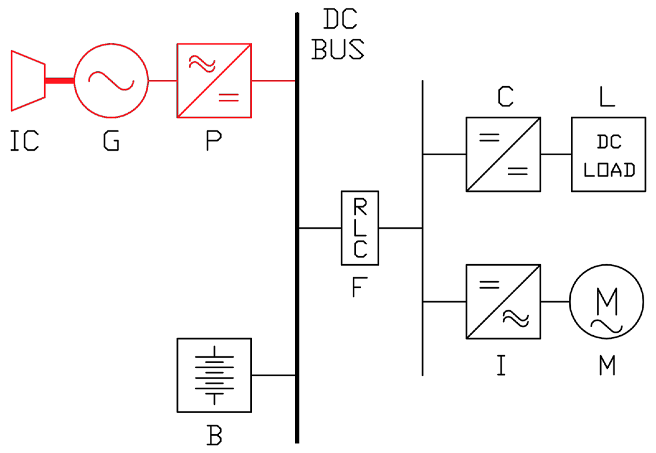
2.1. DC Microgrid Topology

The simplified power system shown in Figure 1 was chosen as a case study to analyze the voltage stability in a floating-bus DC microgrid in presence of a destabilizing CPL. The islanded microgrid used in this study is based on the following elements:

• DC power-generating system, composed of an internal combustion engine (IC), an alternator (G), and a controlled rectifier (P), to supply loads and/or recharge batteries;
• Energy storage system, i.e., an electrochemical battery (B);
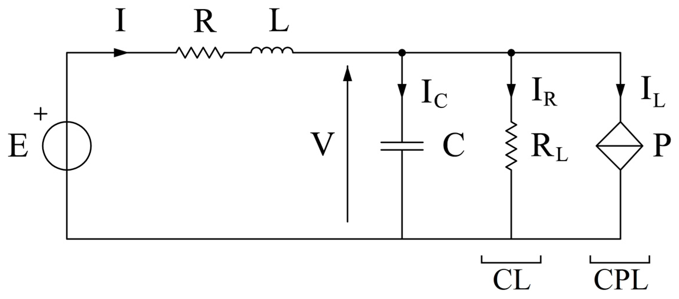
• LC input filter (F), to assure proper voltage and current quality on the load bus;
• Generic static DC load (L), fed by a DC–DC converter (C);
• Generic rotating load (M), supplied by means of a controlled inverter (I).

In order to save space, the system avoids using a battery charger unit, relying upon the controlled rectifier (P) to regulate battery charging. Thus, the DC bus voltage is floating when the power generating system is offline, depending on the battery SoC (the battery is the only source of power). As already shown in Reference [33], in this case voltage stability issues may affect the DC bus. Particular attention has to be paid to the loads; depending on the control bandwidth of the converters used to supply loads from the DC bus, it is possible to classify them into two classes: (i) conventional loads (CLs), and (ii) constant power loads (CPLs). The former category represents loads that do not require strict voltage regulation for proper operation (e.g., resistive heaters, loads with an integrated input conversion stage, etc.). Therefore, their global effect can be modeled through an equivalent linear resistance R_L. Conversely, the latter category is made up of loads requiring tight control by their input power converter (C or I in Figure 1), to either provide a constant voltage (for static loads) or a constant speed/torque (for rotating loads). The final effect is a constant power delivery from the DC bus to the loads. These loads can be modeled through a single equivalent nonlinear current I_L = P/V, where P is the CPL power. It has to be noticed that both static and rotating loads can be classified as CL or CPL, depending on their operating characteristics. The effect of several CLs and CPLs can be modeled using two equivalent aggregated loads. Given the interest in evaluating voltage stability in a floating-bus system, the simplified microgrid shown in Figure 1 was considered as being supplied by batteries only (power system section depicted in black in Figure 1). Thus, it is possible to model the overall power system in battery-only operation using the equivalent circuit of Figure 2, where E is the battery voltage, V is the voltage on the CPL, L and C are the filtering stage components, and R is the inductor physical resistance.

2.2. Definition of Hard Lower Bound for DC Load Voltage

The analysis in Reference [33] introduced the stability problem of a DC floating bus. In particular, an islanded power system supplied only by batteries may be affected by voltage instability in the presence of a perturbation capable of moving the system state outside the BA. This issue becomes critical when the battery has a low SoC and, consequently, its voltage output is low. In this case, the BA shrinks as the bus voltage decreases. This limits the operating margin of the power system.

To introduce the concept of hard lower bound for voltage stability, in this section, the case study was based on the data reported in Reference [33]. The adoption of per unit (p.u.) notation [34] allows performing a numerical continuation analysis [32,33], following the hypothesis of neglecting the presence of the CL (i.e., R_L = ∞). Indeed, the equivalent linear resistance R_L determines an increase in the damping factor, thus enhancing the system’s voltage stability. Conversely, by neglecting CL, it is possible to assess the stability degradation in the worst case [35], thereby making the negative effect of the floating bus more apparent. The method used here to assess voltage stability relies on the evaluation of the basins of attraction (BAs) in the regions close to the stable operating point (Figure 3). Each stable operating point is defined by the couple of variables (v₀, i₀), where v₀ is the steady-state voltage on the capacitor (in p.u.), and i₀ is the steady-state nonlinear current in the filter inductor (in p.u.). The progressive reduction in the battery voltage e (due to the battery SoC decrease) causes the shift of the equilibrium point toward the upper left-hand side of Figure 3 (i.e., lower v₀ and higher current i₀ = p/v₀), with a consequent shrinking in the BA. In particularly, it can be noted that the progressive reduction in BA area (which can be assumed as a measure of system stability) becomes significantly faster for v₀ below 0.8 p.u. (refer to the area with a red boundary in Figure 3). Based on this consideration, it is possible to consider v₀ = 0.8 p.u. as a sort of hard lower bound for the steady-state voltage on the load bus (blue basin of Figure 3). Clearly, this limit on v₀ corresponds to a lower bound also for the battery voltage e, whose value depends on the voltage drop in the filter resistance component. Consequently, for each set of input data (i.e., filter components, CPL power, and rated voltage of the CPL), it is also possible to define a lower limit for the battery SoC, using the voltage limits and the battery specifications.

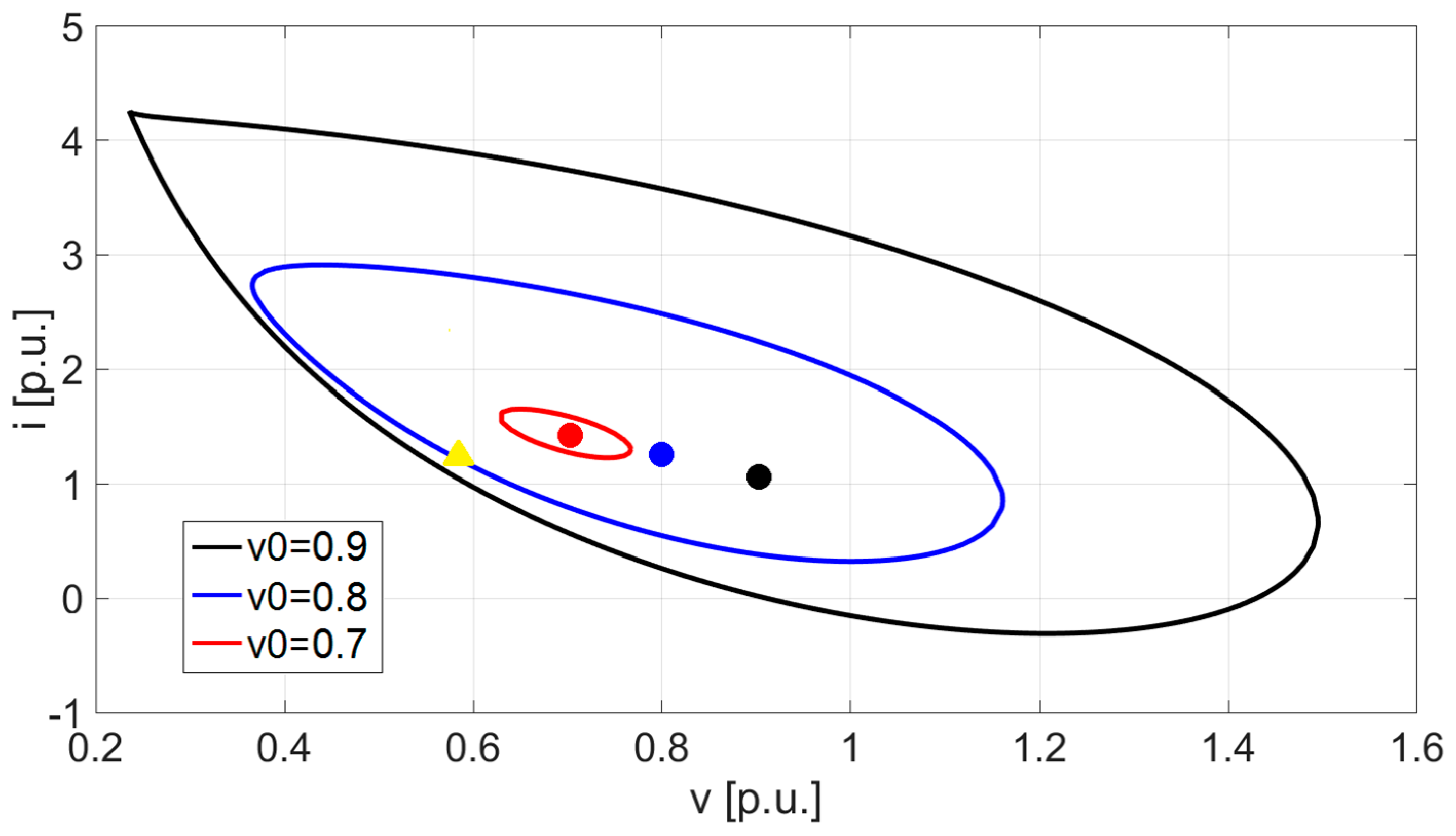
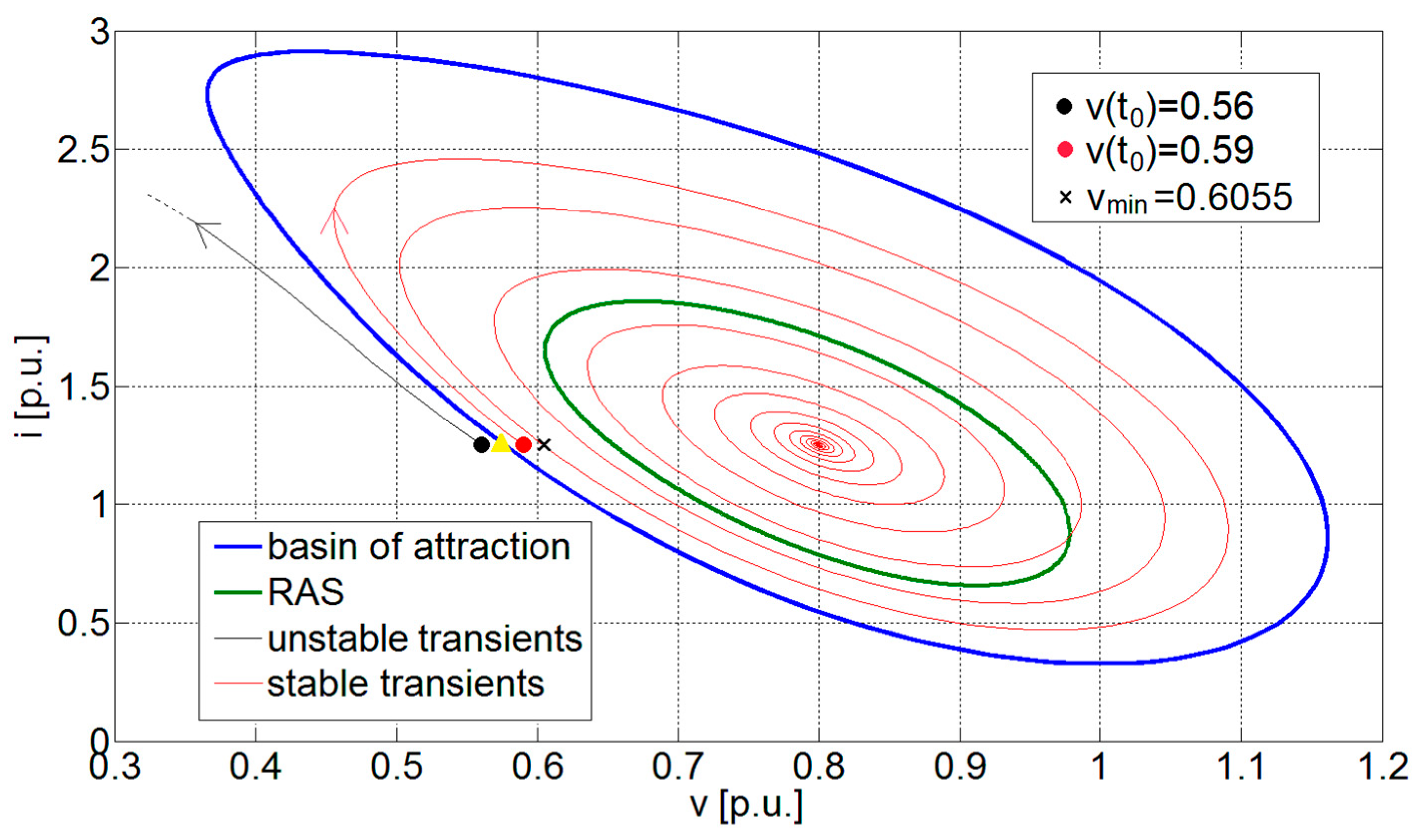
2.3. Basin of Attraction versus Region of Asymptotic Stability

The numerical continuation analysis is a method for studying the stability of nonlinear dynamic systems [32,33]. On the one hand, it allows identifying the Hopf bifurcation [36], which appears when the unstable limit cycle and the equilibrium point coalesce, thus making the equilibrium point unstable. Such a bifurcation was displayed at v₀ = 0.696 p.u. for the case studied in Reference [33]. On the other hand, the numerical continuation analysis makes it possible to evaluate the BA for several different equilibrium points. In fact, it allows determining the lower voltage stability bound once the magnitude of the possible perturbations is known. In particular, in Reference [33], the BA for v₀ = 0.8 p.u. was recognized as the smallest acceptable region for assuring stability in the presence of an impulse perturbation with a reasonable magnitude [37]. Actually, the defined lower bound allows keeping voltage stability after a perturbation constituted by an instantaneous voltage drop of up to ~30% with respect to the actual working point v₀ = 0.8 and i₀ = 1.25 p.u. (i.e., the system state moved to v = 0.5768 p.u. and i = 1.25 p.u.). This can be demonstrated by considering Figure 3, where the perturbed state (yellow triangle) is still in the calculated BA for the starting equilibrium point (blue-bounded area). Conversely, if a lower equilibrium point is assumed (e.g., v₀ = 0.7 p.u., resulting in the red-bounded area in Figure 3), the related BA is so small that the system can be considered unstable for any realistic perturbation.

A different approach to define the stability limits of the system is to establish the region of asymptotic stability (RAS). By applying the Lyapunov theory [38], it is possible to find a conservative region, i.e., the RAS, where a sufficient but not necessary condition for large-signal stability is verified [30]. This, in turn, means that any system state inside the RAS originates a transient that evolves toward a stable equilibrium point. Conversely, system states located outside the RAS are not guaranteed to originate an unstable evolution. Although RAS provides only a subset of the entire BA, its determination is significant. Unlike the BA, which is found numerically, the RAS is defined analytically. Therefore, it is possible to use it in algorithms and control laws able to perform a stability-oriented real-time load management in floating-bus islanded DC microgrids. In particular, the mathematical approach at the basis of the definition of the RAS is used in this paper to define a stability preserving criterion, able to suitably reduce the CPL power when the bus voltage drops. In such a way, the voltage stability is guaranteed even in the presence of low battery voltage output e, i.e., low SoC, assuring the correct supply of the remaining loads.

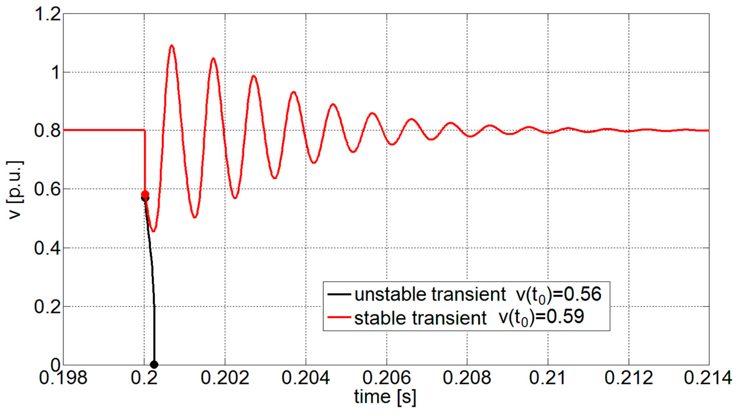
2.4. Numerical Simulation

By removing the conventional load CL from the equivalent circuit in Figure 2, it is possible to define the system’s states as in Equation (1).

$$\{\begin{array}{l}\stackrel{•}{i}=\frac{di}{dt}=\frac{1}{l}\left(e-ri-v\right)\\ \stackrel{•}{v}=\frac{dv}{dt}=\frac{1}{c}\left(i-i_L\right)=\frac{1}{c}\left(i-\frac{p}{v}\right)\end{array},$$

(1)

where v is the CPL voltage, and i is the current flowing in the inductor l. The system parameters were those used in Reference [33], while the CPL power was set at its rated value (i.e., p = 1 p.u.).

Using Matlab Simulink, Equation (1) was implemented to perform simulations to assess the v–i transients following a perturbation. The results were used to provide a dynamic validation of the stability limits previously calculated. The studied DC microgrid in steady-state condition (working point v₀ = 0.8 and i₀ = 1.25 p.u.) was perturbed at t = t₀ = 0.2 s by a voltage impulse capable of instantaneously moving the voltage v applied to the CPL to the new v(t₀) voltage. After the perturbation, the state variables were free to evolve. The study developed in Reference [37] previously demonstrated that this perturbation can be employed for effectively testing the large-signal stability. Therefore, in the following sections, a voltage impulse was considered proper for evaluating the capability offered by the two approaches. The variation in the perturbed initial state v(t₀) allows comparing the consequent v–i transients shown in Figure 4 and Figure 5. In particular, it is possible to notice an unstable behavior when v(t₀) = 0.56 p.u. (black curves), whilst red/green transients (v(t₀) = 0.59 p.u.) are stable and converge toward the pre-disturbance working point. Thus, the performed simulations verified the lower voltage stability limit for the system calculated using BA analyses (v ≈ 0.57 p.u.).

2.5. Validation of Methodological Approach

Dynamic transients are useful for validating both approaches with regards to the large-signal stability, i.e., BA and RAS. To this aim, BA and RAS for the hard lower bound case (i.e., working point v₀ = 0.8 p.u. and i₀ = 1.25 p.u.), together with the dynamic transients after the perturbation, are depicted in the v–i state plane of Figure 6. As can easily be seen, the BA (blue line) can correctly assess system stability. As expected, the transient starting from outside the basin at v(t₀) = 0.56 p.u. (black point) diverges, whereas the red trace of the transient starting inside the basin at v(t₀) = 0.59 p.u. (red point) converges toward the stable working point. Conversely, the RAS (green line) covers only part of the actual BA. This is expected, as the RAS is based only on a sufficient condition. Therefore, it is impossible to predict the system stability through Lyapunov analysis for the transient starting from v(t₀) = 0.59 p.u. (red point).

However, although the RAS can only partially analyze the large-signal behavior, it can constitute a valuable method for designing a stability preserving criterion for floating-bus DC microgrids. Indeed, the determination of the RAS is possible after the identification of the voltage limit above which the Lyapunov first derivative (Equation (2)) is negative.

$$\stackrel{•}{\mathsf{\Psi }}(v)=\frac{1}{lc}\left\{v+rp\frac{1}{v}-e\right\}\cdot \left\{-\frac{r}{l}(v-v_0)-\frac{p}{c}\frac{1}{v}+\frac{p}{c{v}_0}\right\}.$$

(2)

For the microgrid under study, such a limit is expressed by Equation (3).

$$\stackrel{•}{\mathsf{\Psi }}(v)\le 0\iff v\ge \frac{pl}{rc{v}_0}:=v_{\min }.$$

(3)

By assuming the system parameters used in Reference [33]—CPL power p = 1 p.u. and working point v₀ = 0.8 p.u.—the voltage limit v_min = 0.6055 p.u. can be determined (represented by the “×” in Figure 6). Actually, v_min and the basin’s voltage limit (yellow triangle located at v = 0.5768 p.u.) are very close, having a difference smaller than 0.03 p.u. Considering this gap negligible, the voltage limit v_min can act as an effective, yet still conservative, margin for the large-signal stability in the presence of the class of perturbations envisaged in Section 2.4. Moreover, it has to be noted that Equation (3) is a simple equation that can be evaluated immediately, thus making the voltage limit assessment very easy.

3. Stability Preserving Criterion

As previously observed, the system stability is negatively affected by the DC bus voltage decreasing in islanded microgrids feeding a CPL. A possibility for avoiding the consequent instability is to reduce the CPL. In this perspective, a suitably designed CPL management system may be useful for re-establishing a proper stability margin when the bus voltage (which depends on battery SoC in battery-only operation) is low. In order to define such a stability preserving criterion, it is firstly important to understand how the chosen stability index depends on both the CPL power and the floating-bus voltage (Section 3.1). Then, a strategy for decreasing the CPL power can be introduced (see Section 3.2), to guarantee a stable operation even when battery SoC is low. Finally, it is possible to assess the stability performance ensured by the proposed criterion (see Section 3.3) by verifying the presence of a sufficiently large stability region (either BA or RAS) in the v–i state plane as the SoC decreases, and the operating point moves consequently.

3.1. Stability Index

The Lyapunov analysis demonstrated the importance of the v_min term (Equation (3)) in a DC microgrid supplying a CPL. As shown in Figure 6, this parameter represents the lowest voltage margin for a specific DC power system (with given r, l, and c parameters) supplying a CPL with power p and working in steady state at the voltage v₀. In this regard, it is possible to define the distance Δ between the equilibrium point v₀ and the lower bound v_min as a conservative stability index. In fact, any perturbation capable of moving the voltage state inside the area defined by Δ does not jeopardize the system stability, as the Lyapunov conservative condition is still verified.

As previously mentioned, the battery voltage reduction (due to SoC decrease) is responsible for an operating point shift toward the upper left-hand side of the v–i state plane (v₀ decreases and i₀ increases), due to the relationship between supply voltage and absorbed current in a CPL. Moreover, the v₀ drop determines an increase in the v_min limit, as highlighted by Equation (3), which, in turn, leads to a further reduction of Δ. As this behavior is particularly important for the stability issue, the following mathematical study aims to demonstrate the relationship between the bus voltage decrease and the stability index Δ shrinking. To study this issue, it is necessary to define the parameter e_0t, which is the battery voltage needed to supply the CPL rated power (p = 1 p.u.) at the rated load voltage (v₀ = 1 p.u.). This parameter is representative of an optimistic scenario, with a fully charged battery. Conversely, in normal operating conditions, the battery SoC is lower, thus leading to a lower battery voltage e₀, which can be represented as a percentage (e_%) of the full charge voltage e_0t. By observing Figure 2 and assuming the steady-state condition, the battery voltage e₀ is defined through Equation (4).

$$e_0=v_0+r\frac{p}{v_0}=e_{0t}{e}_{\%}.$$

(4)

By rearranging the second equality of Equation (4), it is possible to derive Equation (5), and then obtain the second-order Equation (6) by multiplying Equation (5) with the unknown quantity v₀.

$$v_0-e_{0t}{e}_{\%}+r\frac{p}{v_0}=0.$$

(5)

$$v_0^2-e_{0t}{e}_{\%}{v}_0+rp=0.$$

(6)

By neglecting negative roots, the steady-state voltage v₀ results in Equation (7), while the total battery voltage e_0t is defined in Equation (8), once the rated condition (p = v₀ = 1 p.u.) and full battery (e_% = 1.0) are applied to Equation (4):

$$v_0=\frac{e_{0t}{e}_{\%}+\sqrt{{\left(e_{0t}{e}_{\%}\right)}^2-4rp}}{2}.$$

(7)

$$e_{0t}=1+r.$$

(8)

Assuming a variable e_%, Equations (7) and (8) can be used to delineate the v₀ voltage shift in the presence of different load powers. Consequently, the lower bound v_min corresponding to each v₀ value can be determined using Equation (3), whereas the stability index Δ can be found with Equation (9).

$$\Delta =v_0-v_{\min }=v_0-\frac{pl}{rc{v}_0}.$$

(9)

The equations explained so far allow the drawing of Figure 7, where the gradual contraction of Δ is made evident in response to e_% decrease. In particular, for the system under study, the v₀ curve intersects the v_min trace (i.e., Δ = 0) for e_% ≈ 0.83 in the case of rated power (blue curve). At this specific point, both the large- and the small-signal stability are impaired.

$$\Delta =0\to v_0=v_{\min }\to v_0=\frac{pl}{rc{v}_0}\to v_0=\sqrt{\frac{pl}{rc}}.$$

(10)

On the contrary, for smaller values of CPL power p (black/red curves), larger values of Δ are assured along the e_% drop, thus revealing a possible strategy for ensuring a sufficient stability margin. Actually, it is possible to conceive a smart management of the CPL, able to conveniently decrease its power p as the voltage e₀ decreases, in order to guarantee a proper stability margin.

3.2. Smart CPL Management

As discussed above, when the islanded microgrid is in battery-only operation, a smart management of the CPL power can be useful to preserve voltage stability. To this aim, this subsection focuses on the definition of a power reduction function able to ensure a proper stability index Δ while the battery is discharging (i.e., e_% is decreasing). By multiplying Equation (9) with the steady-state voltage v₀, a second-order equation can be obtained:

$$v_0^2-\Delta v_0-\frac{pl}{rc}=0.$$

(11)

Discarding the negative root, the solution for (11) is

$$v_0=\frac{\Delta }{2}+\sqrt{\frac{{\Delta }^2}{4}+\frac{pl}{rc}}.$$

(12)

The relationship between e₀ and Δ is

$$e_0=v_0+rp\cdot {\left(\frac{\Delta }{2}+\sqrt{\frac{{\Delta }^2}{4}+\frac{pl}{rc}}\right)}^{-1}.$$

(13)

By dividing/multiplying the second term of Equation (13) by the term

$$\left(\frac{\Delta }{2}-\sqrt{\frac{{\Delta }^2}{4}+\frac{pl}{rc}}\right),$$

(14)

a new equation is found as a special product (i.e., difference of two squares):

$$e_0=v_0+\frac{r^{2}cp}{-pl}\left(\frac{\Delta }{2}-\sqrt{\frac{{\Delta }^2}{4}+\frac{pl}{rc}}\right).$$

(15)

Once the v₀ expression (Equation (12)) is substituted into Equation (15), one obtains

$$e_0=\frac{\Delta }{2}+\sqrt{\frac{{\Delta }^2}{4}+\frac{pl}{rc}}-\frac{r^{2}c\Delta }{2l}+\frac{r^{2}c}{l}\sqrt{\frac{{\Delta }^2}{4}+\frac{pl}{rc}},$$

(16)

$$e_0+\left(\frac{r^{2}c}{l}-1\right)\cdot \frac{\Delta }{2}=\left(\frac{r^{2}c}{l}+1\right)\sqrt{\frac{{\Delta }^2}{4}+\frac{pl}{rc}}.$$

(17)

Then, by squaring Equation (17), Equation (18) is obtained and, consequently, after straightforward manipulation, Equations (19) and (20).

$$e_0^2+\left(\frac{r^{2}c}{l}-1\right)\cdot \Delta e_0+{\left(\frac{r^{2}c}{l}-1\right)}^2\cdot \frac{{\Delta }^2}{4}={\left(\frac{r^{2}c}{l}+1\right)}^2\left(\frac{{\Delta }^2}{4}+\frac{pl}{rc}\right),$$

(18)

$$e_0^2+\left(\frac{r^{2}c}{l}-1\right)\cdot \Delta e_0+\left[{\left(\frac{r^{2}c}{l}-1\right)}^2-{\left(\frac{r^{2}c}{l}+1\right)}^2\right]\frac{{\Delta }^2}{4}={\left(\frac{r^{2}c}{l}+1\right)}^2\frac{pl}{rc},$$

(19)

$$e_0^2+\left(\frac{r^{2}c}{l}-1\right)\Delta e_0-\frac{r^{2}c}{l}{\Delta }^2={\left(\frac{r^{2}c}{l}+1\right)}^2\frac{pl}{rc}.$$

(20)

Finally, starting from

$$l{e}_0^2+\left(r^{2}c-l\right)\Delta e_0-r^{2}c{\Delta }^2={\left(r^{2}c+l\right)}^2\frac{p}{rc},$$

(21)

the function p = f(e₀, Δ) can be derived:

$$p=\frac{rc}{{\left(r^{2}c+l\right)}^2}\left[l{e}_0^2+\left(r^{2}c-l\right)\Delta e_0-r^{2}c{\Delta }^2\right].$$

(22)

Equation (22) explains how to modify the CPL power p to maintain a desired Δ when e₀ becomes lower.

To better analyze Equation (22), the filter parameters r, l, and c may be gathered in the K term,

$$K=\frac{{\tau }_L}{{\tau }_C}=\frac{l}{r}\cdot \frac{1}{rc}=\frac{l}{r^{2}c},$$

(23)

through the definition of the time constants τ_L and τ_C. The K term allows simplifying Equation (22).

$$p=\frac{rc}{{\left(r^{2}c\right)}^2{\left(1+K\right)}^2}\left[K{r}^{2}c{e}_0^2+r^{2}c\left(1-K\right)\Delta e_0-r^{2}c{\Delta }^2\right];$$

(24)

$$p=\frac{K{e}_0^2+\left(1-K\right)\Delta e_0-{\Delta }^2}{r{\left(1+K\right)}^2}.$$

(25)

Finally, by substituting the e₀ voltage definition in Equation (4) into Equation (25), one obtains

$$p=\frac{e_{\%}^2\left[e_{0t}^{2}K\right]+e_{\%}\left[\Delta e_{0t}^{}(1-K)\right]-{\Delta }^2}{r{\left(1+K\right)}^2}.$$

(26)

Such a function, equivalent to Equation (22), better highlights the relationship between voltage and power. For this reason, it can be called the “power function”. Through Equation (26), it is possible to appreciate the reduction in CPL power needed to migrate the working point (i.e., a decrease in i₀) toward a new point with the given (desired) stability index Δ (Figure 8). In particular, the green curve in Figure 8 is related to the power reduction function capable of guaranteeing the rated stability index, whereas greater/smaller values of Δ are ensured when the power reduction follows the red/blue curves. Clearly, if the requested stability index exceeds the rated value (0.6 vs. 0.516, red curve), then the rated power is not reachable even with a fully charged battery. Conversely, the DC microgrid can feed the rated CPL power with a partially charged battery (e.g., e_% = 0.95) if the stability performance is downgraded (0.4 vs. 0.516, blue curve). As stated in References [11,12,13,14,15,16,17,18,19,20], the stability of a DC power system supplying a CPL is closely related to the filter parameters. For this reason, Figure 9 depicts the influence of the parameter K on the power function. In particular, by halving K (i.e., the capacitance c is doubled with respect to the inductance l, keeping the resistance r constant), the range of voltages in which the rated power can be supplied is extended (blue curve). On the contrary, more critical scenarios are given by a double K (red curve), where the DC microgrid can never provide the rated power to the CPL while keeping voltage stability (i.e., p < 0.5 p.u. when e_% = 0.9).

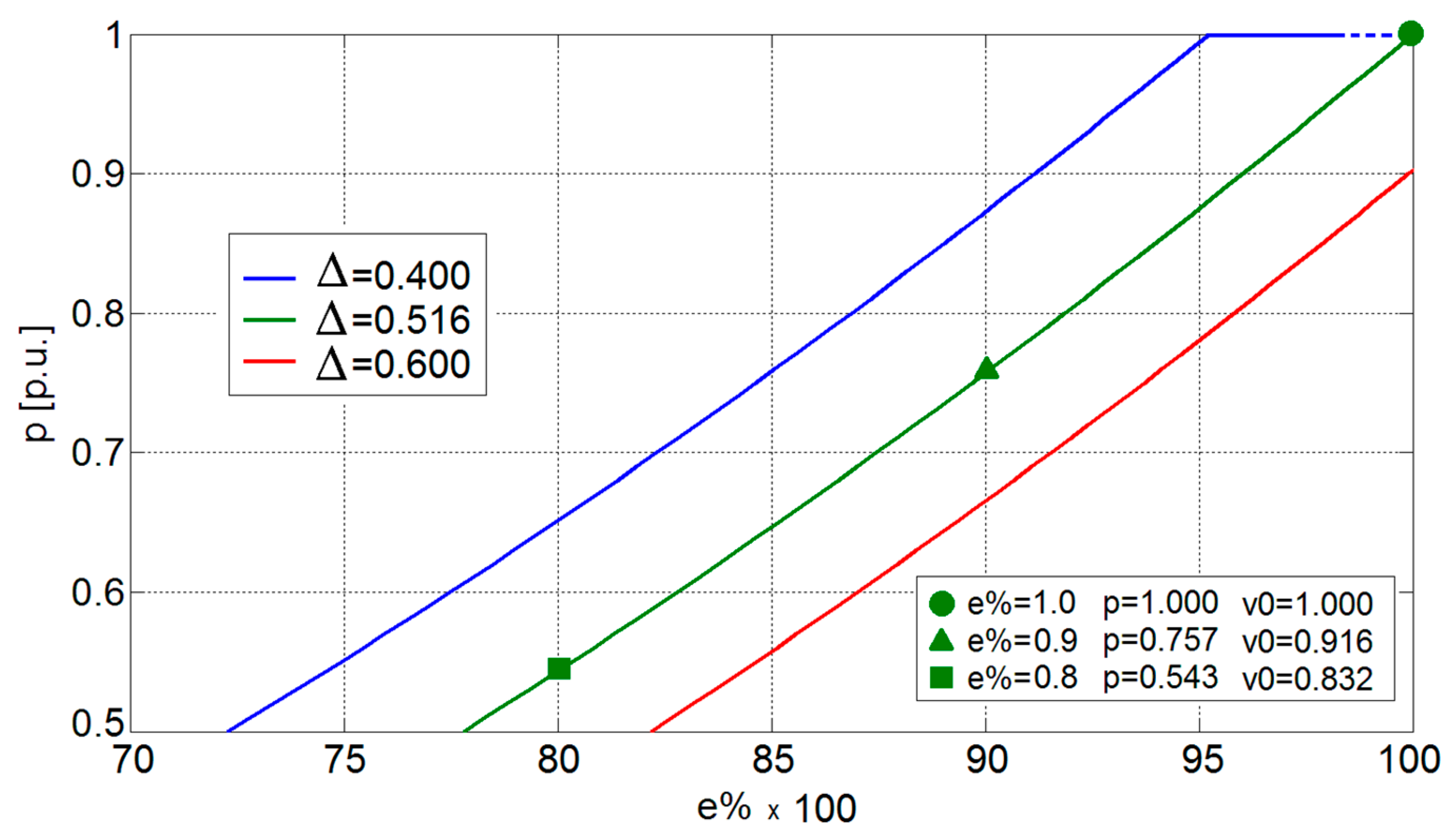
3.3. Migration of RAS and BA

The effects of the proposed power reduction function on RASs and BAs of the system are depicted in Figure 10 and Figure 11, respectively. As expected, both RAS and BA shift along the v–i plane, as e_% and p diminish. Moreover, their area remains constant, due to the stability index invariance (Δ = 0.516) guaranteed by applying the proposed power reduction function.

4. Application Example

To demonstrate the applicability of the proposed smart CPL management (see Section 3.2) and to test the possible outcomes of the power derating on system performance, an application example was chosen. Specifically, a full electric vehicle was selected. The electric propulsion motor and its inverter constitute the CPL. Such a choice allows clearly showing the impact on performance of the proposed smart CPL management by evaluating indices that are evident and easy to understand (i.e., maximum achievable speed and 0–100 km/h acceleration time).

In order to study the worst case for DC voltage stability, the power system of the application example was simplified by removing the CLs and considering battery-only operation. Thus, a battery, an LC filter, and a CPL (the propulsion system) constituted the power system to be analyzed. The result was an islanded DC microgrid with a floating bus, similar to the one analyzed in the previous Sections. The data of a commercial electric car (2011 Nissan Leaf) were inferred from several online datasheets, and are shown in

Table 1. Application example: electric vehicle parameters. SoC—state of charge.

Electric motor power	Pn	80 kW
Battery capacity		24 kWh
Nominal battery voltage		360 V
Battery voltage at full charge		403 V
Battery voltage at 20% SoC		336 V
Mass	M	1500 kg
Frontal area	A	2.28 m2
Wheel diameter (205/55 R16)	R	63.16 cm
Maximum speed (unlimited)		170 km/h
Maximum speed (software limited)		144 km/h
0–100 km/h (unofficial tests)		~9 s
Aerodynamic penetration coefficient	Cx	0.32

. Using standard physics equations and applying a set of simplifying hypotheses, a Matlab script was developed in order to evaluate the performance of the car with respect to the CPL power. As previously mentioned, the maximum achievable speed and the 0–100 km/h acceleration time were chosen as performance indices. Proper modeling was applied to allow the calculation of these indices starting from available propulsion power. To lower the modeling burden, the vehicle was considered as a point of mass, free from the influence of external forces (e.g., no height variations and no wind), whereas the propulsion motor and inverter system had a control bandwidth so high with respect to the overall vehicle that time constants could be considered negligible. As previously discussed, CPL power has to be decreased through the application of the power reduction function (Equation (26)), to preserve the DC voltage stability when the battery discharge causes a decrease in the bus voltage. In particular, the maximum battery voltage range was defined by means of Table 1 parameters: 403 V voltage at full charge means e_% = 1, while 336 V at 20% SoC corresponds to e_% = 0.83. For what concerns the stability index, the value Δ = 0.516 was chosen as a feasible tradeoff between a wide stability margin and the applicable CPL power (as shown in Figure 8, green trace). Using these data, the reduced CPL power can be determined through Equation (26), leading to the results depicted in

Table 2. Application example: power reduction function effect and resulting power at the wheels.

Battery Voltage (%)	Electric Motor Power (per Unit)	Electric Motor Power (kW)	Wheels Power (kW)
100	1	80.00	68.00
95	0.875	70.00	59.50
90	0.757	60.56	51.48
85	0.646	51.68	43.93
80	0.543	43.44	36.92

. Focusing on the performance indices, the maximum achievable speed can be determined by exploiting the steady-state force equilibrium equation,

$$F_m=F_f+F_a,$$

(27)

where F_m is the force applied by the electric motor to the wheels, F_f the force due to the wheel–road friction, and F_a is the drag force due to the air. These three forces were assessed by considering the additional system parameters reported in

Table 3. Application example: system parameters.

Static friction coefficient (rubber–asphalt) wet conditions	μs	0.5
Rolling friction coefficient (rubber–asphalt)	μd	0.035
Traction control safety coefficient	ktc	0.75
Power loss (from motor to wheels)		15%
Minimum battery SoC		20%
Air density (kg/m3)	r0	1.29

. In particular, to model the overall transmission losses, the wheel traction was calculated by reducing the electric motor power through a 15% loss coefficient, thus resulting in a wheel power ranging from 37 to 68 kW (Table 2). Conversely, the wheel–road friction F_f and the air drag force F_a were determined using the following equations:

$$F_f={\mu }_{d}RMg,$$

(28)

$$F_a=\frac{1}{2}\left(r_{0}A{C}_x{v}^2\right),$$

(29)

where the parameters are defined in Table 1, Table 2 and Table 3, whilst v is the car speed in m/s, and g the gravity acceleration constant. Finally, the maximum achievable speed was calculated as a function of the power at the wheels using Equations (27)–(29), the results of which are shown in Figure 12 (red curve, left ordinate).

On the other hand, the 0–100 km/h acceleration time can be found by means of the dynamic equation:

$$a(v)=\frac{1}{2M}\left[F_{md}(v)-F_f-F_a(v)\right],$$

(30)

where a(v) is the vehicle acceleration, F_a(v) the drag force due to the air, and F_md(v) is the dynamic force applied by the electric propulsion motor to the wheels.

In particular, by taking into account not only the propulsion motor’s available power (Table 2), but also the maximum force transferrable from wheels to the asphalt in bad weather conditions and a traction control safety coefficient (refer to Table 3), the term F_md may be obtained.

$$F_{md}(v)=\{\begin{array}{c}{F}_m(v)if{F}_m\le F_{\lim }\\ F_{\lim }if{F}_m>F_{\lim }\end{array},$$

(31)

$$F_{\lim }=\frac{2}{4}{k}_{tc}{\mu }_{s}gM,$$

(32)

where F_lim represents the maximum force transferrable from wheels to the asphalt by a four-by-two-wheel drive car. It is worth noting that, in Equation (30), all the terms depend on speed. Therefore, corresponding to a series of different propulsion power values, Equation (30) was used to calculate the vehicle speed variation from zero to its maximum. The resulting dataset, which relates vehicle speed and time for each power value, allows evaluating the 0–100 km/h time with a simple search algorithm. The results of this procedure are shown in Figure 12 (blue curve, right ordinate), where the acceleration time is shown with respect to the power available at the wheels.

By analyzing Figure 12, it is possible to evaluate the effect of the proposed smart CPL management on the performance indices for the application example. Firstly, the maximum achievable speed at the minimum available power is still in the range of the maximum speed limit set by the car software (135 km/h achievable vs. 144 km/h limit). Secondly, the acceleration performance at the lowest battery level is still satisfactory (~10.4 s) with respect to common car performance levels. In this regard, it has to be noted that these results were calculated in a worst-case condition, thus possibly leading to lower performance loss in a real system.

Although these results were obtained by oversimplifying both the power system and the system’s physics (i.e., not constituting a complete performance assessment), they may provide important insight into the stability criterion effect. Actually, considering the application example, the proposed criterion can represent a valuable solution for preserving the DC stability by suitably managing the CPL power without excessively impairing the system performance. Obviously, the applicability of the proposed smart CPL management depends not only on the single system under study, but also on some parameters that can be defined accordingly by designers (such as coefficient K and stability margin Δ).

5. Conclusions

The paper proposed a smart power limitation in order to preserve system stability in a DC microgrid feeding a CPL. Such a management is crucial when the battery is the only power source for the microgrid. The battery operation determines a floating DC bus, whose unregulated voltage varies over time depending on the SoC of the battery. When the battery SoC is decreasing, i.e., the DC bus voltage is diminishing, the stability region shrinking can be evaluated by means of the Lyapunov theory and numerical continuation analysis. The analytical method demonstrated its effectiveness in defining the stability index, which has the main role in the definition of the stability preserving criterion. For a given power-quality filter, the power function expresses the mathematical relationship among bus voltage, stability index, and CPL power. Therefore, a proper management can be designed to limit the power of the CPL to assure stability when the steady-state DC bus voltage decreases. This power reduction was analyzed on the basis of several results, which confirm the invariance of both the area and shape of the stability regions (i.e., RASs and BAs), while the operating point moves in the state plane. The paper finally demonstrated the effectiveness of the proposed criterion by means of a suitable application example.

References

1. Hansen, J.F.; Wendt, F. History and State of the Art in Commercial Electric Ship Propulsion, Integrated Power Systems, and Future Trends. Proc. IEEE 2015, 103, 2229–2242. [Google Scholar] [CrossRef]
2. Emadi, A. Transportation 2.0. IEEE Power Energy Mag. 2011, 9, 18–29. [Google Scholar] [CrossRef]
3. Zubieta, L.E. Are Microgrids the Future of Energy? DC Microgrids from Concept to Demonstration to Deployment. IEEE Electrif. Mag. 2016, 4, 37–44. [Google Scholar] [CrossRef]
4. Patterson, B.T. DC, Come Home: DC Microgrids and the Birth of the “Enernet”. IEEE Power Energy Mag. 2012, 10, 60–69. [Google Scholar] [CrossRef]
5. IEEE Std. 1709-2010. IEEE Recommended Practice for 1 to 35 kV Medium Voltage DC Power Systems on Ships; IEEE: Piscataway, NJ, USA, 2010. [Google Scholar]
6. Meng, L.; Shafiee, Q.; Trecate, G.F.; Karimi, H.; Fulwani, D.; Lu, X.; Guerrero, J.M. Review on Control of DC Microgrids and Multiple Microgrid Clusters. IEEE J. Emerg. Sel. Top. Power Electron. 2017, 5, 928–948. [Google Scholar]
7. Jin, Z.; Sulligoi, G.; Cuzner, R.; Meng, L.; Vasquez, J.C.; Guerrero, J.M. Next-Generation Shipboard DC Power System: Introduction Smart Grid and dc Microgrid Technologies into Maritime Electrical Netowrks. IEEE Electrif. Mag. 2016, 4, 45–57. [Google Scholar] [CrossRef] [Green Version]
8. Emadi, A.; Williamson, S.S.; Khaligh, A. Power Electronics Intensive Solutions for Advanced Electric, Hybrid Electric, and Fuel Cell Vehicular Power Systems. IEEE Trans. Power Electron. 2006, 21, 567–577. [Google Scholar] [CrossRef]
9. Dragičević, T.; Lu, X.; Vasquez, J.C.; Guerrero, J.M. DC Microgrids—Part I: A Review of Control Strategies and Stabilization Techniques. IEEE Trans. Power Electron. 2016, 31, 4876–4891. [Google Scholar]
10. Dragičević, T.; Lu, X.; Vasquez, J.C.; Guerrero, J.M. DC Microgrids—Part II: A Review of Power Architectures, Applications, and Standardization Issues. IEEE Trans. Power Electron. 2016, 31, 3528–3549. [Google Scholar] [CrossRef] [Green Version]
11. Kwasinski, A.; Onwuchekwa, C.N. Dynamic behavior and stabilization of DC microgrids with instantaneous constant-power loads. IEEE Trans. Power Electron. 2011, 26, 822–834. [Google Scholar] [CrossRef]
12. Emadi, A.; Khaligh, A.; Rivetta, C.H.; Williamson, G.A. Constant power loads and negative impedance instability in automotive systems: Definition, modeling, stability and control of power electronic converters and motor drives. IEEE Trans. Veh. Technol. 2006, 55, 1112–1125. [Google Scholar] [CrossRef]
13. Rahimi, A.M.; Emadi, A. Active Damping in DC/DC Power Electronic Converters: A Novel Method to Overcome the Problems of Constant Power Loads. IEEE Trans. Ind. Electron. 2009, 56, 1428–1439. [Google Scholar] [CrossRef]
14. Rahimi, A.M.; Williamson, G.A.; Emadi, A. Loop-Cancellation Technique: A Novel Nonlinear Feedback to Overcome the Destabilizing Effect of Constant-Power Loads. IEEE Trans. Veh. Technol. 2010, 59, 650–661. [Google Scholar] [CrossRef]
15. Bosich, D.; Giadrossi, G.; Sulligoi, G. Voltage control solutions to face the CPL instability in MVDC shipboard power systems. In Proceedings of the AEIT Annual Conference 2014, Trieste, Italy, 18–19 September 2014. [Google Scholar]
16. Sulligoi, G.; Bosich, D.; Giadrossi, G.; Zhu, L.; Cupelli, M.; Monti, A. Multiconverter Medium Voltage DC Power Systems on Ships: Constant-Power Loads Instability Solution using Linearization via State Feedback Control. IEEE Trans. Smart Grid 2014, 5, 2543–2552. [Google Scholar] [CrossRef]
17. Cupelli, M.; Ponci, F.; Sulligoi, G.; Vicenzutti, A.; Edrington, C.S.; El-Mezyani, T.; Monti, A. Power Flow Control and Network Stability in an All-Electric Ship. Proc. IEEE 2015, 103, 2355–2380. [Google Scholar] [CrossRef] [Green Version]
18. Bosich, D.; Sulligoi, G.; Mocanu, E.; Gibescu, M. Medium Voltage DC Power Systems on Ships: An Offline Parameter Estimation for Tuning the Controllers’ Linearizing Function. IEEE Trans. Energy Convers. 2017, 32, 748–758. [Google Scholar] [CrossRef]
19. Hossain, E.; Perez, R.; Nasiri, A.; Padmanaban, S. A Comprehensive Review on Constant Power Loads Compensation Techniques. IEEE Access 2018, 6, 33285–33305. [Google Scholar] [CrossRef]
20. Su, M.; Liu, Z.; Sun, Y.; Han, H.; Hou, X. Stability Analysis and Stabilization Methods of DC Microgrid with Multiple Parallel-Connected DC–DC Converters Loaded by CPLs. IEEE Trans. Smart Grid 2018, 9, 132–142. [Google Scholar] [CrossRef]
21. Riccobono, A.; Santi, E. Comprehensive Review of Stability Criteria for DC Power Distribution Systems. IEEE Trans. Ind. Appl. 2014, 50, 3525–3535. [Google Scholar] [CrossRef]
22. Riccobono, A.; Cupelli, M.; Monti, A.; Santi, E.; Roinila, T.; Abdollahi, H.; Arrua, S.; Dougal, R.A. Stability of Shipboard DC Power Distribution: Online Impedance-Based Systems Methods. IEEE Electrif. Mag. 2017, 5, 55–67. [Google Scholar] [CrossRef]
23. Javaid, U.; Freijedo, F.D.; Dujic, D.; van der Merwe, W. Dynamic Assessment of Source–Load Interactions in Marine MVDC Distribution. IEEE Trans. Ind. Electron. 2017, 64, 4372–4381. [Google Scholar] [CrossRef] [Green Version]
24. Belkhayat, M.; Cooley, R.; Witulski, A. Large Signal Stability Criteria for Distributed Systems with Constant Power Loads. In Proceedings of the 26th IEEE Annual Power Electronics Specialists Conference, Atlanta, GA, USA, 18–22 June 1995; pp. 1333–1338. [Google Scholar]
25. Griffo, A.; Wang, J.; Howe, D. Large Signal Stability Analysis of DC Power Systems with Constant Power Loads. In Proceedings of the IEEE Vehicle Power and Propulsion Conference (VPPC), Harbin, China, 3–5 September 2008; pp. 1–6. [Google Scholar]
26. Herrera, L.; Zhang, W.; Wang, J. Stability Analysis and Controller Design of DC Microgrids with Constant Power Loads. IEEE Trans. Smart Grid 2017, 8, 881–888. [Google Scholar]
27. Aboushady, A.A.; Ahmed, K.H.; Finney, S.J.; Williams, B.W. Lyapunov-based high-performance controller for modular resonant DC/DC converters for medium-voltage DC grids. IET Power Electron. 2017, 10, 2055–2064. [Google Scholar] [CrossRef]
28. Mukherjee, N.; Strickland, D. Control of Cascaded DC–DC Converter-Based Hybrid Battery Energy Storage Systems—Part II: Lyapunov Approach. IEEE Trans. Ind. Electron. 2016, 63, 3050–3059. [Google Scholar] [CrossRef] [Green Version]
29. Kabalan, M.; Singh, P.; Niebur, D. Large Signal Lyapunov-Based Stability Studies in Microgrids: A Review. IEEE Trans. Smart Grid 2017, 8, 2287–2295. [Google Scholar] [CrossRef]
30. Bosich, D.; Gibescu, M.; Sulligoi, G. Large-signal stability analysis of two power converters solutions for DC shipboard microgrid. In Proceedings of the 2017 IEEE Second International Conference on DC Microgrids (ICDCM), Nuremburg, Germany, 27–29 June 2017; pp. 125–132. [Google Scholar]
31. Sulligoi, G.; Bosich, D.; Giadrossi, G. Linearizing voltage control of MVDC power systems feeding constant power loads: Stability analysis under saturation. In Proceedings of the 2013 IEEE Power & Energy Society General Meeting, Vancouver, BC, Canada, 21–25 July 2013. [Google Scholar]
32. Grillo, S.; Musolino, V.; Sulligoi, G.; Tironi, E. Stability enhancement in DC distribution systems with constant power controlled converters. In Proceedings of the IEEE 15th International Conference on Harmonics and Quality of Power (ICHQP), Hong Kong, China, 17–20 June 2012; pp. 848–854. [Google Scholar]
33. Bosich, D.; Giadrossi, G.; Sulligoi, G.; Grillo, S.; Tironi, E. More Electric Vehicles DC Power Systems: A Large Signal Stability Analysis in presence of CPLs fed by Floating Supply Voltage. In Proceedings of the IEEE International Electric Vehicle Conference (IEVC), Florence, Italy, 17–19 December 2014; pp. 1–6. [Google Scholar]
34. Chen, M.; Rincón-Mora, G.A. Accurate Electrical Battery model capable of predicting runtime and I-V performance. IEEE Trans. Energy Convers. 2006, 21, 504–511. [Google Scholar] [CrossRef]
35. Rahimi, A.M.; Emadi, A. An Analytical Investigation of DC/DC Power Electronic Converters with Constant Power Loads in Vehicular Power Systems. IEEE Trans. Veh. Technol. 2009, 58, 2689–2702. [Google Scholar] [CrossRef]
36. Kuznestov, Y.A. Elements of Applied Bifurcation Theory, 3rd ed.; Springer: New York, NY, USA, 2004. [Google Scholar]
37. Arcidiacono, V.; Monti, A.; Sulligoi, G. Generation control system for improving design and stability of medium-voltage DC power systems on ships. IET Electr. Syst. Transp. 2012, 2, 158–167. [Google Scholar] [CrossRef]
38. Khalil, H.K. Nonlinear Systems; Prentice Hall: Upper Saddle River, NJ, USA, 1992. [Google Scholar]
Figure 1. Proposed direct current (DC) microgrid; the power system section in battery-only operation is shown in black.
Applsci 08 02102 g001
Figure 2. DC microgrid equivalent circuit model.
Applsci 08 02102 g002
Figure 3. Basins of attraction (BAs) corresponding to shifted equilibrium points.
Applsci 08 02102 g003
Figure 4. Voltage transients due to a voltage impulse perturbation at t = 0.2 s.
Applsci 08 02102 g004
Figure 5. Current transients due to a voltage impulse perturbation at t = 0.2 s.
Applsci 08 02102 g005
Figure 6. BA and region of asymptotic stability (RAS); validation when v0 = 0.8 p.u.
Applsci 08 02102 g006
Figure 7. Stability index Δ, with varying constant power load (CPL) power and DC bus voltage.
Applsci 08 02102 g007
Figure 8. Power reduction function for preserving different values of stability index Δ.
Applsci 08 02102 g008
Figure 9. Power reduction function in the presence of different filtering solutions.
Applsci 08 02102 g009
Figure 10. RAS migration imposed by power reduction function.
Applsci 08 02102 g010
Figure 11. BA migration imposed by power reduction function.
Applsci 08 02102 g011
Figure 12. Maximum achievable speed and 0–100 km/h acceleration time as a function of power at the wheels.
Applsci 08 02102 g012