Article

Deep Learning Case Study for Automatic Bird Identification

1
Signal Processing Laboratory, Tampere University of Technology, 28101 Pori, Finland
2
Mathematics Laboratory, Tampere University of Technology, 28101 Pori, Finland
*
Author to whom correspondence should be addressed.
This paper is an extended version of our paper published in 2017 International Symposium ELMAR
Current address: Tampere University of Technology, Signal Processing Laboratory, P.O. Box 300, 28101 Pori, Finland.
Appl. Sci. 2018, 8(11), 2089; https://doi.org/10.3390/app8112089
Submission received: 27 September 2018 / Revised: 22 October 2018 / Accepted: 23 October 2018 / Published: 29 October 2018
(This article belongs to the Special Issue Advanced Intelligent Imaging Technology)

Abstract

:
An automatic bird identification system is required for offshore wind farms in Finland. Indubitably, a radar is the obvious choice to detect flying birds, but external information is required for actual identification. We applied visual camera images as external data. The proposed system for automatic bird identification consists of a radar, a motorized video head and a single-lens reflex camera with a telephoto lens. A convolutional neural network trained with a deep learning algorithm is applied to the image classification. We also propose a data augmentation method in which images are rotated and converted in accordance with the desired color temperatures. The final identification is based on a fusion of parameters provided by the radar and the predictions of the image classifier. The sensitivity of this proposed system, on a dataset containing 9312 manually taken original images resulting in 2.44 × 10⁶ augmented data set, is 0.9463 as an image classifier. The area under receiver operating characteristic curve for two key bird species is 0.9993 (the White-tailed Eagle) and 0.9496 (The Lesser Black-backed Gull), respectively. We proposed a novel system for automatic bird identification as a real world application. We demonstrated that our data augmentation method is suitable for image classification problem and it significantly increases the performance of the classifier.

1. Introduction

Several offshore wind farms are under construction on the Finnish west coast. The official environmental specifications define that bird species behaviour at the vicinity of wind turbines must be monitored. This concerns especially two species: the White-tailed Eagle (Haliaeetus albicilla) and the Lesser Black-backed Gull (Larus fuscus fuscus), which are explicitly mentioned in the environment license. The only way to fulfil this demand cost efficiently is to automate monitoring, and that requires automatic bird species identification at such a level that the aforementioned bird species are separable from all other species in the study area. The problem is how to identify bird species in flight automatically in real-time? The prototype system for automated bird identification is developed and placed at a test location on Finnish west coast. This system is still under construction.
The ultimate objective of bird monitoring in wind farms is to find suitable methods for collision detection [1,2], and especially to find possible deterrent methods [3]. The WT-Bird of the Energy Research Centre of the Netherlands is the first (i.e., known to us) published research of this subject. The principle of the WT-Bird system is that a bird collision could be detected by the sound of the impact and that the bird species can be recognised by non-real time method from video footage [4,5]. However, it has known problems with false alarms in high wind circumstances concerning larger bird species and it has no automated species identification algorithm [6].
Radar is a feasible choice for the detection of birds since the identification need is restricted to the flying birds only. If merely a radar is used, the identification capability is limited to a few size classes according to radar suppliers. Obviously, external information is required and a conceivable method is to exploit visual camera images, thus a digital single-lens reflex (DSLR) camera with a telephoto lens is applied. This paper shows that convolutional neural network (CNN) with deep learning algorithm trained on real-world images is capable to achieve sufficient state-of-the-art performance as an image classifier. At present, all the images are manually taken at the test location. The images will be acquired automatically by the final system.

2. Hardware

2.1. Radar System

We have used a radar system supplied by Robin Radar Systems B.V. (The Haag, Netherlands) because they provide an avian radar system that is able to detect birds. They also have tracker algorithms for tracking a detected object over time i.e., between the blips. The model we use is the ROBIN 3D FLEX v1.6.3 and it is actually a combination of two radars and a software package for implementation of various algorithms such as the tracking algorithms [7].

2.2. Video Head Control

We have used the PT-1020 motorized video head supplied by 2B Security Systems (Copenhagen, Denmark) [8]. The video head is operated by Pelco-D control protocol [9] and the control software for it is developed by us with C in Linux Ubuntu 16.04 platform. The video head steering is based on height, latitude and longitude coordinates (WGS84) provided by the radar. No coordinate conversion from one system to another is needed because all calculations are performed in WGS84 system. However, the geographical coordinates are converted to the rectangular coordinates in accordance with the Finnish Geodetic Institute [10].

2.3. Camera Control

We have manually collected the images at the test site with a Canon 7D mark II camera (Tokyo, Japan) and a Canon 500/f4 IS telephoto lens (Tokyo, Japan). The software for controlling the camera is developed with C# in Microsoft Visual Studio 14.0 because this is the only environment supported by the Canon API at present. The Canon API library of EDSDKLib-1.1.2 is applied. The code is developed in accordance with the instructions and functions of the API. The Canon API library is available for application on the Internet [11].

3. Data Processing

3.1. Input Data

Input data for the identification system consist of digital images and parameters from the radar. The parameters from the radar are real numbers such as velocity of a flying bird in m/s and bearing (i.e., a heading: the horizontal angle between the direction of an object and that of true north) in degrees. All images for training the CNN are of wild birds in flight and they have been taken manually at the test location. There are also constraints concerning the area where the images have to be taken. Here, the area refers to the air space in the vicinity of the pilot wind turbine. We have used the wind turbine swept area (the diameter of the swept area is 130 m) as a suitable altitude level constraint for taking the images, because birds flying below or above the swept area are not in danger. At this stage, the images are only taken in the vicinity of 1350 m in lengthwise direction, which is the distance to the pilot wind turbine. There are 1164 images for each class and the number of classes is 8, thus the original training set size is 8×1164 = 9312. We applied data augmentation as it is well-known method to increase performance of an image classifier. In addition, the original (i.e., not augmented) data set includes plenty of data examples of images with various portion of cloudiness as the background and also with clear sky as the background.
The number of images of each class should be the same as a CNN is applied [12] and therefore the lowest number of images of the classes is used. The number of classes (which includes both key species) is 8 at this phase. The eight classes for training the CNN are the Common Goldeneye (Bucephala clangula), the White-tailed Eagle (Haliaeetus albicilla), the Herring Gull (Larus argentatus), the Common Gull (Larus canus, the Lesser Black-backed Gull (Larus fuscus fuscus), the Black-headed Gull (Larus ridibundus, the Great Cormorant (Phalacrocorax carbo) and Common/Arctic Tern (Sterna hirundo/paradisaea).

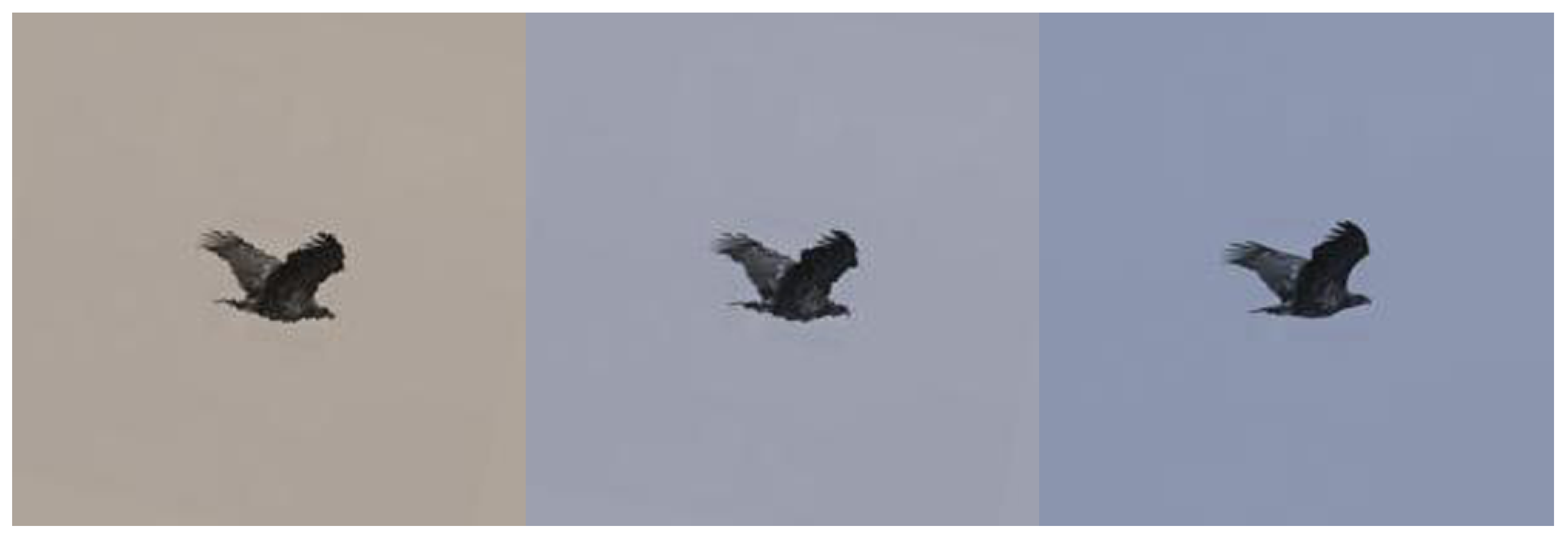
3.2. Data Augmentation

Our system is operating in natural environment and therefore prevailing weather has significant influence on the tonality of the images taken at the test site. Obviously, the lighting will be different in a different time of a day and a different time of a year, and thus the toning of the images will be changing according to lighting. Color temperature is a property of a light source. It is the temperature of the ideal black-body radiator that radiates light of the same color as the corresponding light source. In this context black-body radiation is the thermal electromagnetic radiation emitted by a black body. A black-body is an opaque and non-reflective body. It has a specific spectrum and intensity that depends only on the temperature of the black-body, and it is assumed to be uniform and constant. In our case, the light source is the sun that closely approximates a black-body radiator. Even though the color of the sun may appear different depending on its position, the changing of color is mainly due to the scattering of light and it is not because of the changes in the black-body radiation [13,14,15,16]. Color matching functions (CMFs) provide the absolute energy values of three primary colors which appear the same as each spectrum color. We applied the International Commission on Illumination (Commission internationale de l’éclairage, CIE) 10-deg color matching functions in our data augmentation algorithm [17].
The data augmentation is done according to the curves in Figure 1. Ref. [18] by converting an image into different color temperatures between 2000 K and 15,000 K with step size s, where s ϵ {50, 75, 100, 150, 200, 250, 300, 1000}. This makes the training set significantly larger, e.g., if s is 50, a class containing 1164 training examples becomes a class of 261 × 1164 = 303,804 examples + the original image. The augmented data set size as a result of various value of s is given in Table 1 for the original data set of size 8 × 1164 = 9312. After color conversion, the images are rotated by a random angle between −20 and 20 drawn from the uniform distribution. This value has been altered from 30 to 20 since our first publication because it was empirically noticed that the target birds had never a position angled this steep. Motivation for image rotation is CNN’s property of being invariant to small translations but not rotation of an image [19].
Examples of one original image and two images as an output of the augmentation algorithm with this original image as an input and s = 200 are presented in Figure 2. The color temperature of the original image is 7600 K and the two augmented images 5600 K and 9600 K , respectively.

4. The Proposed System

The most important role of the radar is to detect flying birds, but it also provides parameters for bird identification (i.e., classification) [20,21]. The parameters provided by the radar system are: the distance in 3D of a target (m), the velocity of a target (m/s) and the trajectory of a target. The distance of a detected bird is used to estimate the size of the bird in meters. Velocity of a target bird is used for the final classification. The system also includes the aforementioned camera with the telephoto lens and a motorized video head. The camera is controlled by the application programmable interface (API) of the camera manufacturer. The system has three servers: the radar server, the video head steering server and the camera control server. Software for the radar server is supplied by the manufacturer of the radar but the software for the other two servers is result of our development work.
We took series of images of a single target bird and each image is processed according to the schematic diagram of the system in Figure 3.
Segmentation is computed in parallel to image classification in order to obtain an estimate of the target bird size in pixels, i.e., despite that segmentation is computed simultaneously when the classification process is started, it is not part of the actual classification, but the result of the segmentation is used for assigning a value to the size estimate parameter. When the estimate in pixels is known, the target bird size estimate in meters can be calculated. We studied methods from simple threshold to fuzzy logic for solving the problem at hand i.e., a dark figure against bright background and vice versa as well. At the extremity, the background and the target can share several colors in the RGB color space. We achieved the best results by applying fuzzy logic segmentation compared to the threshold segmentation and the edge detection segmentation [22,23]. In particular, we applied Mamdani’s fuzzy inference method [24]. Figure 4a,b show an example of segmentation.

5. Classification

The classification process is presented in Figure 5. Series of images of a single target (i.e., as a sequence of temporally consecutive frames of the same bird) are fed to the CNN that is applied to feature extraction. The two-step learning method is applied, i.e., the CNN is trained with the first N-1 layers viewed as feature maps and these maps are used to train a Support Vector Machine (SVM) classifier [25]. The SVM classifier makes use of one-versus-all binary learners, in which, for each binary learner, one class is positive and the rest are negative. The total number of the binary learners is the same as the number of classes. A linear classification model is applied. Stochastic gradient descent with 10 as the mini-batch size, and the Hinge loss function with regularization term 1/n, where n is a number of training examples [26,27] are also applied. The output of the SVM is presented as P-vectors as follows:
P i = [ c 1 , c 2 , ... , c nc ] , i = 1 , ... , n ,
where c j is a probability of belonging to class j, nc is the number of classes and n is the number of images in each series, thus there will be one P-vector for each image in any given image series.
There are also two parameters based on information provided by the radar system. The size of the target bird is estimated as follows. The frame size ([width x height y], in pixels) of the camera and the angle of view ( α ) of the lens are known. The distance (d) to the target bird is provided by the radar. The maximum number of horizontal ( σ h ) and vertical ( σ v ) pixels of the target bird are calculated from the segmented image, respectively. The angle of view, b, at the distance, d, is calculated over a right-angled triangle (see Figure 6). The horizontal number of pixels/meter is given by
ρ h = x b h ,
and the vertical number of pixels/meter by
ρ v = y b v ,
where, b h and b v denote the horizontal and the vertical angles of view, respectively. The estimate for the size of the bird in a single image in square meters as an area of rectangle is:
e = σ h ρ h σ v ρ v .
The size estimate is presented as a vector with elements placed according to the class order (the classes are ordered alphabetically by their names), i.e., class 1, class 2, … class nc, where nc denotes the number of classes. The composition of the vector is following: calculate the average of the size estimates of the image series, check from the size-look-up table all the classes that contain the average size, e, turn those elements to one and set the others to zero, yielding
Size Estimate , E = [ e 1 , e 2 , ... , e nc ] ,
with elements:
e j = 1 , if e fits class j , 0 , otherwise .
The velocity of the target bird is composed in similar way as the E-vector in Size Estimate (5), i.e., check from the velocity-look-up table all the classes that contain the provided velocity, v , turn those elements to one and the others to zero.
Velocity , V = [ v 1 , v 2 , ... , v nc ] ,
with elements:
v j = 1 , if v fits class j , 0 , otherwise .
The final classification is achieved by a fusion between the parameters provided by the radar and the predictions from the image classifier. The combined P-vector for a series of images is:
Combined P -vector , P = i = 1 n P i ,
where n is the number of images in each series and the fusion vector, Φ , is:
Fusion vector , Φ = P . V . E ,
where “.∗” denotes element wise multiplication. The score, S , for final prediction is:
Prediction , S = max j ( Φ ) ,
j = arg max j ( Φ ) ,
where j is the index of the predicted class.

5.1. Convolutional Neural Network

The CNN network architecture is presented in Figure 7. The architecture of the CNN results in (200 − 12 + 2 × 1)/2 + 1 = 96 for one side of the feature map and as of the result of square feature maps there are 96 × 96 = 9216 neurons in each feature map of the first convolution layer. Note that there is no max-pooling layer between the first and the second convolution layers. Motivation for this is that we wanted all of the finest edges to be included in resulting feature maps.
The input image is normalized and zero-centered before feeding it to the network. CNN with Mini-batch training and supervised mode as well as stochastic gradient descent with momentum is applied [28,29,30,31]. The L2 Regularization (i.e., weight decay) method for reducing over-fitting is also applied [30,31,32]. Due to limited capacity of computer resources the network size in terms of free parameters is kept small, thus resulting in total of 92 feature maps which are extracted by convolution layers with kernel sizes [ 12 × 12 × 3 ] × 12 , [ 3 × 3 × 12 ] × 16 and [ 3 × 3 × 16 ] × 64 , respectively. Total number of weights is about 9.47 × 10⁶.
Each convolution layer is followed by a Rectified Linear Units (ReLU) nonlinearity layer [33], which simply applies a threshold operation,
f ( x ) = 0 x < 0 , x x 0 ,
to all the components of its input. This non-saturating nonlinearity in deep CNN makes the training several times faster when applied together with the hyperbolic tangent sigmoid transfer function [33,34]. Cross Channel Normalization layers follow the first and the second ReLU layers. These layers aid the generalization as their function may be seen as brightness normalization [34].
The purpose of max-pooling layer is to build robustness to small distortions. This is achievable by filtering over local neighbourhoods as follows: divide the input into rectangular pooling regions, and compute the maximum of each region, thus performing downsampling and reducing the overfitting as well [35].
There are three fully-connected layers at the end of the network for making final nonlinear combinations of features, and prediction by the last fully-connected layer followed by softmax activation which produces a distribution over the class labels with cross entropy loss function [31].

5.2. Hyperparameter Selection
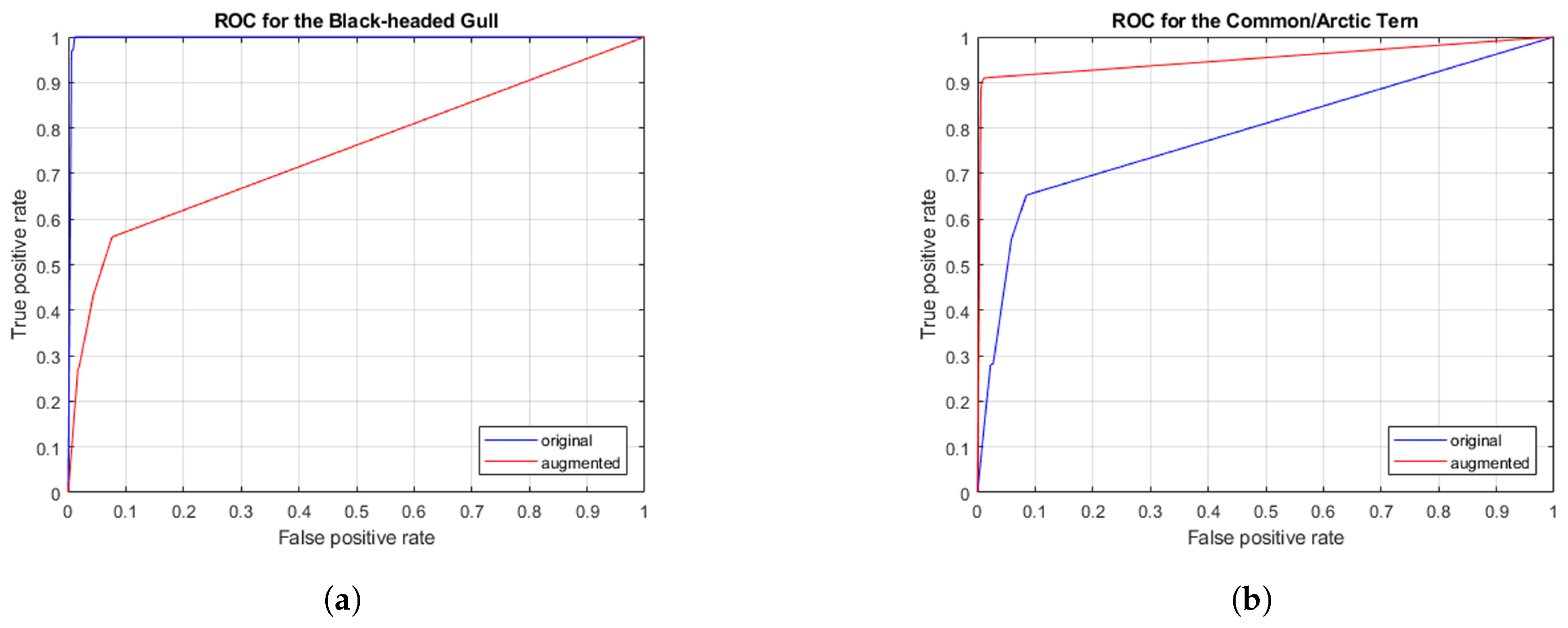
The split into a training set and a validation set was 70% and 30%, respectively. The initial weights for all layers were drawn from the Gaussian distribution with mean 0 and standard deviation 0.01. Initial biases were set to zero. The L2 value was set to 0.0005 and mini-batch size was set to 128. The values of all the previously mentioned hyperparameters were fixed and we used manual tuning only for choosing the combination of the number of epochs and the learning rate drop period (LRDP). Two models with different values of the two parameters were trained on the original data set (i.e., no data augmentation applied). One model was trained on the augmented data set with s = 1100 and s = 350, respectively. Several models with various values of the two parameters were trained on the augmented data set with s = 200 and s = 50, respectively. The results of training these models are presented in Table 2, in which performance is presented as true positive rate (TPR, i.e., sensitivity). The initial values of the two parameters applied to training on each data set are selected empirically. As a result of running these tests, the best model in terms of performance is the model trained on the augmented data set with s = 50 (i.e., 2,439,744 training examples), the number of epochs = 8, and the LRDP = 3.
Initial learning rate was set to 0.01 and when the same value was applied to the number of epochs and the LRDP the learning rate was kept constantly at its initial value. The learning rate decay schedule (LRDS) was applied when the values of the number of epochs and the LRDP were different of each other. In the LRDS method, the learning rate is dropped by a factor of 0.1 (i.e., the updated learning rate will be the current learning rate × 0.1) when a given number of epochs is reached. This given number of epochs is the effective value of the LRDP. Motivation for using the LRDS method is as training proceeds with shorter leaps on the loss function surface from some point on, the optimal value for the weights (i.e., in terms of performance as a classifier) can be found more accurately. If only the short leaps would be applied, the number of epochs should be very large, thus resulting in significant increase of training time. The challenge is to find the points from where on the learning rate should be reduced. We approached this problem in two ways. We fixed the LRDP value and altered the number of epochs. Initially, the problem was to find a suitable starting value for the LRDP. It was intuitively clear that the LRDP value should increase as the number of epochs increases. A small value of the LRDP combined with a high value of the number of epochs would lead to substantial underfitting. We also fixed the number of epochs and altered the LRDP value instead. The same initial value problem concerns this approach as well. However, the size of the respective data set should give some guidance for choosing the initial values. Moreover, as the number of training examples increases, the number of epochs should decrease in order to avoid overfitting.
We applied the dropout technique for improving the performance of our CNN [34,36]. We trained models with fixed hyperparameter values with and without the dropout technique. If overfitting occurs, the results in terms of classification performance should be better as the dropout technique is applied compared to those models for which it is not applied. These tests indicate that some overfitting occurs when the models were trained on the augmented data sets but not necessarily on the original data sets. The dropout was implemented after the first and the second fully-connected layers by randomly setting the output neurons to zero with a probability of 0.5.

6. Results

The following results are based on manually taken images at the test site. The images have been taken at the same position where the camera will be installed. We trained two models on the original data set and several models on four different augmented data sets, in which s was 50, 200, 350 and 1100, respectively (see Table 2). The models with s ϵ {350,1100} were trained only for testing the data augmentation algorithm. The effect of the data augmentation algorithm on classification performance is presented in Figure 8.
The best performance (in TPR) of the two models trained on the original data set is 0.7362. Performance for the models trained on the augmented data sets varies between 0.8687 and 0.9984, which shows clear improvement as the augmented training set size increases and especially compared to the models trained on the original set. Training with and without the dropout technique implied that overfitting will occur to some extent as the data augmentation is applied and the dropout technique decreases this overfitting. The results were different for the original data sets, in which case overfitting was insignificant. These results are logical due to the fact that the enhancement in performance obtained by the data augmentation is extracted from the original images, and thus it inevitably increases redundancy. The results for the original data sets imply that the number of training examples was simply not large enough.
We tested generalization of the models on 100 unseen images for each class, i.e., the data set for testing the models was 8·100,100 = 600 images that the models have never seen before. According to these tests the system achieves its state-of-the-art performance of 0.9463 with the augmented data set of the size 2.44 × 10⁶ (i.e., the color conversion step size, s = 50), number of epochs 8, LRDP 3, and the dropout applied.
The receiver operating characteristic (ROC) curves and the area under the curve (AUC) for the 8 classes (i.e., bird species) are presented in Figure 9, Figure 10, Figure 11 and Figure 12. The TPR values of the generalization tests are applied in these figures. The red curve is for the augmented data set and the blue curve is for the original data set.

7. Discussion

We assembled the non-deep (i.e., in terms of the number of the convolution layers, 3) CNN for image classification, and demonstrated that the model is suitable for real-world application, especially, when the number of training data is limited. We presented and demonstrated that our data augmentation method improves significantly the performance of the classifier, and the desirable state-of-the-art performance as an image classifier can be achieved by applying it. Thus, we showed that the data augmentation is crucial for the classification performance. We also showed that our model generalizes well to images never seen before and hence it is applicable for real-world problem. The number of images in the original data set have been increased since our first publication resulting in the better state-of-the-art performance of 0.9463 compared to the first result of 0.9100. It is noteworthy that this better result is achieved despite of the increased number of the classes, i.e., 8 compared to 6 [37].
The measured performance of the image classifier has been obtained without using the parameters supplied by the radar. It is obvious that those parameters (i.e., the E- and V-vectors) provide additional and relevant a-priori knowledge to the system and they can turn a misclassified (by images) class into the correct one. Data collection will be continued at the test site resulting in a larger original data set, and thus hopefully better performance of the classifier. The number of classes will increase as more images of scarcer species are collected.
We are currently working on the collision detection problem, but no collisions have been observed until now while the pilot wind turbine has been manually monitored for 30 months. It seems that collisions are quite rare in the research area and this makes the field testing of the possible collision detection methods challenging. More research is required of possible deterrent methods, especially on species or species group level.
We proposed a novel system for automatic bird identification as a real world application. However, the system has restrictions such as images can not be taken in pitch-dark or in poor visibility conditions. Infrared cameras may contribute to the collision detection, but their contribution to classification is poor because all color information is lost. The proposed system is still in the installation phase, so we have not yet been able to test the complete system.

Author Contributions

Conceptualization, J.N.; Data Curation, J.N.; Formal Analysis, J.N.; Funding Acquisition, J.T.T.; Investigation, J.N.; Methodology, J.N.; Project Administration, J.N.; Software, J.N.; Supervision, J.T.T.; Validation, J.T.T.; Visualization, J.N.; Writing—Original Draft, J.N.; Writing—Review and Editing, J.T.T.

Funding

This research received no external funding.

Acknowledgments

The authors wish to thank Suomen Hyötytuuli for the financial support of purchasing necessary equipment and Robin Radar Systems for the technical support with the applied radar system.

Conflicts of Interest

The authors declare no conflict of interest.

Abbreviations

The following abbreviations are used in this manuscript:
APIApplication programmable interface
AUCArea under the curve
CIECommission internationale de l’éclairage
CMFsColor matching functions
CNNConvolutional neural network
DSLRdigital single-lens reflex camera
LDPRLearning rate drop period
LRDSLearning rate decay schedule
ReLURectified linear units
ROCReceiver operating characteristic
SVMSupport vector machine
TPRTrue positive range

References

  1. Desholm, M.; Kahlert, J. Avian Collision Risk at an Offshore Wind Farm. Biol. Lett. 2008, 1, 296–298. [Google Scholar] [CrossRef] [PubMed]
  2. Marques, A.T.; Rodrigues, S.; Costa, H.; Pereira, M.J.R.; Fonseca, C.; Mascarenhas, M.; Bernardino, J. Understanding bird collisions at wind farms: An updated review on the causes and possible mitigation strategies. Biol. Conserv. 2014, 179, 40–52. [Google Scholar] [CrossRef]
  3. Baxter, A.T.; Robinson, A.P. A comparison of scavenging bird deterrence techniques at UK landfill sites. Int. J. Pest Manag. 2007, 53, 347–356. [Google Scholar] [CrossRef]
  4. Verhoef, J.P.; Westra, C.A.; Korterink, H.; Curvers, A. WT-Bird A Novel Bird Impact Detection System. Available online: www.ecn.nl/docs/library/report/2002/rx02055.pdf (accessed on 27 September 2018).
  5. Wiggelinkhuizen, E.J.; Barhorst, S.A.M.; Rademakers, L.W.M.M.; den Boon, H.J. Bird Collision Monitoring System for Multi-Megawatt Wind Turbines, WT-Bird: Prototype Development and Testing. Available online: www.ecn.nl/publications/PdfFetch.aspx?nr=ECN-E--06-027 (accessed on 27 September 2018).
  6. Wiggelinkhuizen, E.J.; den Boon, H.J. Monitoring of Bird Collisions in Wind Farm under Offshore-like Conditions Using WT-BIRD System: Final Report. Available online: www.ecn.nl/docs/library/report/2009/e09033.pdf (accessed on 27 September 2018).
  7. Robin Radar Models. Available online: https://www.robinradar.com/ (accessed on 27 September 2018).
  8. PT1020 Video Head. Available online: http://www.2bsecurity.com/product/pt-1020-medium-sized-pan-tilt/ (accessed on 27 September 2018).
  9. Bruxy REGNET for Pelco-D Protocol. Available online: http://bruxy.regnet.cz/programming/rs485/pelco-d.pdf (accessed on 27 September 2018).
  10. Häkli, P.; Puupponen, J.; Koivula, H. Suomen Geodeettiset Koordinaatistot Ja Niiden VäLiset Muunnokset. Natl. Land Surv. Finl. 2009. Available online: https://www.maanmittauslaitos.fi/sites/maanmittauslaitos.fi/files/fgi/GLtiedote30korjausliite.pdf (accessed on 27 September 2018).
  11. Canon’s European Developer Programmes. Available online: https://www.developers.canon-europa.com/developer/bsdp/bsdp_pub.nsf (accessed on 27 September 2018).
  12. Hensman, P.; Masko, D. The Impact of Imbalanced Training Data for Convolutional Neural Networks. Available online: https://www.kth.se/social/files/588617ebf2765401cfcc478c/PHensmanDMasko_dkand15.pdf (accessed on 27 September 2018).
  13. Speranskaya, N.I. Determination of spectrum color co-ordinates for twenty-seven normal observers. Opt. Spectrosc. 1959, 7, 424–428. [Google Scholar]
  14. Stiles, W.S.; Burch, J.M. NPL colour-matching investigation: Final report. Opt. Acta 1959, 6, 1–26. [Google Scholar] [CrossRef]
  15. Wyszecki, G.; Stiles, W.S. Color Science: Concepts and Methods, Quantitative Data and Formulae, 2nd ed.; John Wiley & Sons Inc.: New York, NY, USA, 1982; ISBN 978-0471021063. [Google Scholar]
  16. Stockman, A.; Sharpe, L.T. Spectral sensitivities of the middle- and long-wavelength sensitive cones derived from measurements in observers of known genotype. Vis. Res. 2000, 40, 1711–1737. [Google Scholar] [CrossRef]
  17. CIE. CIE Proceedings, Vienna Session; Committee Report E-1.4.1; CIE: Paris, France, 1963; pp. 209–220. [Google Scholar]
  18. Blackbody Color Datafile. Available online: www.vendian.org/mncharity/dir3/blackbody/UnstableURLs/bbr_color.html (accessed on 27 September 2018).
  19. Goodfellow, I.; Bengio, Y.; Courville, A. Deep Learning; MIT Press: Cambridge, MA, USA, 2016; Available online: www.deeplearningbook.org (accessed on 27 September 2018).
  20. Richards, M.A. Fundamentals of Radar Signal Processing; The McGraw-Hill Companies: New York, NY, USA, 2005; ISBN 0-07-144474-2. [Google Scholar]
  21. Bruderer, B. The Study of Bird Migration by Radar, part1: The Technical Basis. Naturwissenschaften 1997, 84, 1–8. [Google Scholar] [CrossRef]
  22. The MathWorks, Inc. Fuzzy Logic Toolbox Documentation. Available online: https://se.mathworks.com/help/fuzzy/fuzzy.pdf. (accessed on 27 September 2018).
  23. Yuheng, S.; Hao, J. Image Segmentation Algorithms Overview. Available online: https://arxiv.org/ftp/arxiv/papers/1707/1707.02051.pdf (accessed on 27 September 2018).
  24. Mamdani, E.H.; Assilian, S. An experiment in linguistic synthesis with a fuzzy logic controller. Int. J. Man-Mach. Stud. 1975, 7, 1–13. [Google Scholar] [CrossRef]
  25. Huang, J.F.; LeCun, Y. Large-Scale Learning with Svm and Convolutional Nets for Generic Object Categorization. Available online: http://yann.lecun.com/exdb/publis/pdf/huang-lecun-06.pdf (accessed on 27 September 2018).
  26. Moore, R.C.; DeNero, J. L1 and L2 regularization for multiclass hinge loss models. In Proceedings of the Symposium on Machine Learning in Speech and Language Processing, Bellevue, WA, USA, 27 June 2011. [Google Scholar]
  27. Duan, K.B.; Keerthi, S.S. Which Is the Best Multiclass SVM Method? An Empirical Study. Mult. Classif. Syst. LNCS 2005, 3541, 278–285. [Google Scholar] [Green Version]
  28. LeCun, Y.; Bottou, L.; Bengio, Y.; Haffner, P. Gradient-based learning applied to document recognition. Proc. IEEE 1998, 86, 2278–2324. [Google Scholar] [CrossRef] [Green Version]
  29. Li, M.; Zhang, T.; Chen, Y.; Smola, A.J. Efficient Mini-batch Training for Stochastic Optimization. In Proceedings of the 20th ACM SIGKDD international conference on Knowledge, New York, NY, USA, 24–27 August 2014; pp. 661–670, ISBN 978-1-4503-2956-9. [Google Scholar]
  30. Murphy, K.P. Machine Learning: A Probabilistic Perspective; The MIT Press: Cambridge, MA, USA, 2012; ISBN 978-0-262-01802-9. [Google Scholar]
  31. Bishop, C.M. Pattern Recognition and Machine Learning; Jordan, M., Kleinberg, J., Schölkopf, B., Eds.; Springer: New York, NY, USA, 2006; ISBN 0-387-31073-8. [Google Scholar]
  32. Haykin, S. Neural Networks: A Comprehensive Foundation, 2nd ed.; Prentice Hall/Pearson: New York, NY, USA, 1994; p. 470. ISBN 0-13-908385-5. [Google Scholar]
  33. Nair, V.; Hinton, G.E. Rectified linear units improve restricted boltzmann machines. In Proceedings of the 27th International Conference on Machine Learning, Haifa, Israel, 21–24 June 2010; pp. 807–814. [Google Scholar]
  34. Krizhevsky, A.; Sutskever, I.; Hinton, G.E. Imagenet classification with deep convolutional neural networks. Adv. Neural Inf. Process. Syst. 2012, 25. [Google Scholar] [CrossRef]
  35. Jarrett, K.; Kavukcuoglu, K.; Ranzato, M.A.; LeCun, Y. What is the best multi-stage architecture for object recognition. In Proceedings of the International Conference on Computer Vision, Kyoto, Japan, 29 Septemer–2 October 2009; pp. 2146–2153. [Google Scholar]
  36. Srivastave, N.; Hinton, G.E.; Krizhevsky, A.; Sutskever, I.; Salakhutdinov, R. Dropout: A Simple Way to Prevent Neural Networks from Overfitting. J. Mach. Learn. Res. 2014, 15, 1929–1958. [Google Scholar]
  37. Niemi, J.; Tanttu, J.T. Automatic Bird Identification for Offshore Wind Farms: A Case Study for Deep Learning. In Proceedings of the 59th IEEE International Symposium ELMAR-2017, Zadar, Croatia, 18–20 September 2017. [Google Scholar] [CrossRef]
Figure 1. Color temperature and corresponding red, blue and green (RGB) values presented according to Commission Internationale de l’Eclairage (CIE) 1964 10-degree color matching function.
Applsci 08 02089 g001
Figure 2. Data example of the White-tailed Eagle. The image on the left is an augmented image with the color temperature 5600 K . The original image is in the middle with color temperature 7600 K . The image on the right is an augmented image with the color temperature 9600 K .
Applsci 08 02089 g002
Figure 3. Schematic diagram of the system.
Applsci 08 02089 g003
Figure 4. Example of binary image acquired by the segmentation process. (a) an original image of the Herring Gull; (b) respective binary image as a result of segmentation of the original image.
Applsci 08 02089 g004
Figure 5. The classification process.
Applsci 08 02089 g005
Figure 6. Diagram of the size estimate calculation.
Applsci 08 02089 g006
Figure 7. The architecture of the convolutional neural network. The letters, s, and, p, in the max-pooling layers denote stride and padding, respectively. In convolution layers, the first two numbers in the square brackets indicate the width and hight of the respective convolution kernel and the third number is the depth. The number before the brackets is the number of feature maps in respective convolution layer.
Applsci 08 02089 g007
Figure 8. The red curve is for validation during training and the blue curve is according to the generalization test. The actual True Positive Rate (TPR) values are used with s ϵ {350,1100}, and the average TPR value is used of the models with s ϵ {50,200}, respectively. The starting value for both curves is the average value of the two models trained on the original data set.
Applsci 08 02089 g008
Figure 9. ROC curves for the White-tailed Eagle and the Lesser Black-backed Gull. (a) AUC for the original data set and for the augmented data set is 0.9137 and 0.9993, respectively; (b) AUC for the original data set and for the augmented data set is 0.7460 and 0.9496, respectively.
Applsci 08 02089 g009
Figure 10. ROC curves for the Herring Gull and the Common Gull. (a) AUC for the original data set and for the augmented data set is 0.6926 and 0.9128, respectively; (b) AUC for the original data set and for the augmented data set is 0.6967 and 0.9644, respectively.
Applsci 08 02089 g010
Figure 11. ROC curves for the Black-headed Gull and the Common/Artic Tern. (a) AUC for the original data set and for the augmented data set is 0.7583 and 0.9972, respectively; (b) AUC for the original data set and for the augmented data set is 0.8111 and 0.9508, respectively.
Applsci 08 02089 g011
Figure 12. ROC curves for the Great Cormorant and the Common Goldeneye. (a) AUC for the original data set and for the augmented data set is 0.8853 and 0.9870, respectively. (b) AUC for the original data set and for the augmented data set is 0.0.8807 and 0.9829, respectively.
Applsci 08 02089 g012
Table 1. Number of images for augmented data set with various step, s, values.
Step, sNumber of Images for One ClassNumber of Images for 8 Classes
110015,132121,056
70023,280186,240
35045,396363,168
20077,988623,904
100153,6481,229,184
50304,9682,439,744
Table 2. Convolutional Neural Network (CNN) performance (with the Support Vector Machine (SVM) as an actual classifier) as a result of various number of epochs and Learning Rate Drop Period (LRDP).
Number of Training ExamplesNumber of EpochsLRDPTPR TrainingTPR Generalization
931230300.71750.6995
931260600.73620.7052
121,05625100.86870.8662
363,1681870.91370.9187
623,90412120.97880.9253
623,90416160.98390.9254
623,90424240.98350.9170
623,9041650.98300.9270
623,9041660.98310.9337
623,9041690.98340.9249
623,90416130.98370.9154
2,439,744330.99600.9246
2,439,744550.99710.9313
2,439,744880.99840.9363
2,439,74412120.99840.9296
2,439,744530.99650.9250
2,439,744830.99830.9463
2,439,7441030.99840.9448
2,439,7441230.99830.9425

