SambotII: A New Self-Assembly Modular Robot Platform Based on Sambot

Featured Application

This manuscript developed a new self-assembly modular robot (SMR) system SambotII and provided a new vision-based method for efficient and accurate autonomous docking of SMRs. The present work lays a foundation for the future research of modular and swarm robots. Based on the present hardware and software platforms, complex behaviors and various tasks can be achieved on SambotII in the future, such as environment exploration, path planning, robotic swarm control, morphology control and, etc.

Abstract

A new self-assembly modular robot (SMR) SambotII is developed based on SambotI, which is a previously-built hybird type SMR that is capable of autonomous movement and self-assembly. As is known, SambotI only has limited abilities of environmental perception and target recognition, because its STM-32 processor cannot handle heavy work, like image processing and path planning. To improve the computing ability, an x86 dual-core CPU is applied and a hierarchical software architecture with five layers is designed. In addition, to enhance its perception abilities, a laser-camera unit and a LED-camera unit are employed to obtain the distance and angle information, respectively, and the color-changeable LED lights are used to identify different passive docking surfaces during the docking process. Finally, the performances of SambotII are verified by docking experiments.

1. Introduction

1.1. Background

A self-assembly or self-reconfiguration modular robot (SMR) system is composed of a collection of connected modules with certain degrees of locomotion, sensing, and intercommunication [1,2,3]. When compared with robots that have fixed topologies, SMR systems have some advantages, such as versatility, robustness, and low cost [4].

The concept of dynamically self-reconfigurable robotic system was firstly proposed by Toshio Fukuda in 1988 [5]. Since then, many interesting robot systems have been proposed. In spite of the significant advances of SMRs, researchers in this field believe that there is a gap between the state-of-art research on modular robots and their real-world applications [3]. As Stoy and Kurokawa [6] stated, the applications of self-reconfigurable robots are still elusive.

One main challenge in this field is how to achieve autonomous docking among modules, especially with higher efficiency and accuracy. Autonomous docking is an essential capability for the system to realize self-reconfiguration and self-repairing in completing operational tasks under complex environments. Various methods, such as the infrared-red (IR) ranging, vision-based ranging, ultrasonic ranging, etc., have been employed to guide the autonomous docking process.

The IR-based methods generally have high accuracy, simple structure and small size. Thus, they are suitable for self-reconfigurable robotic systems with the shapes of chain, tree or lattices. They were applied in many SMR systems, like PolyBot [7], ATRON [8], ModeRED [9], SYMBRION [10], etc. However, the IR-based methods are unsuitable for mobile robotic systems due to the limited detection ranges.

The vision-based methods can provide more information than IR-based method do. Some SMR systems like CKBot [11], M-TRAN [12], and UBot [13] utilize the vision-based methods in their autonomous docking process. However, these methods generally involve large-scale and complex image processing and information extraction. This restricts their applications in SMR systems, to some extent.

Except the IR and vision-based methods, ultrasonic sensors are also used in the docking process. For example, the JL-2 [14] conducts autonomous docking under the guidance of several ultrasonic sensors. In addition, the eddy-current sensors, hall-effect sensors and capacitance meters are occasionally applied in the docking navigation. However, they are easy to be interfered by motors and metallic objects.

1.2. Related Works

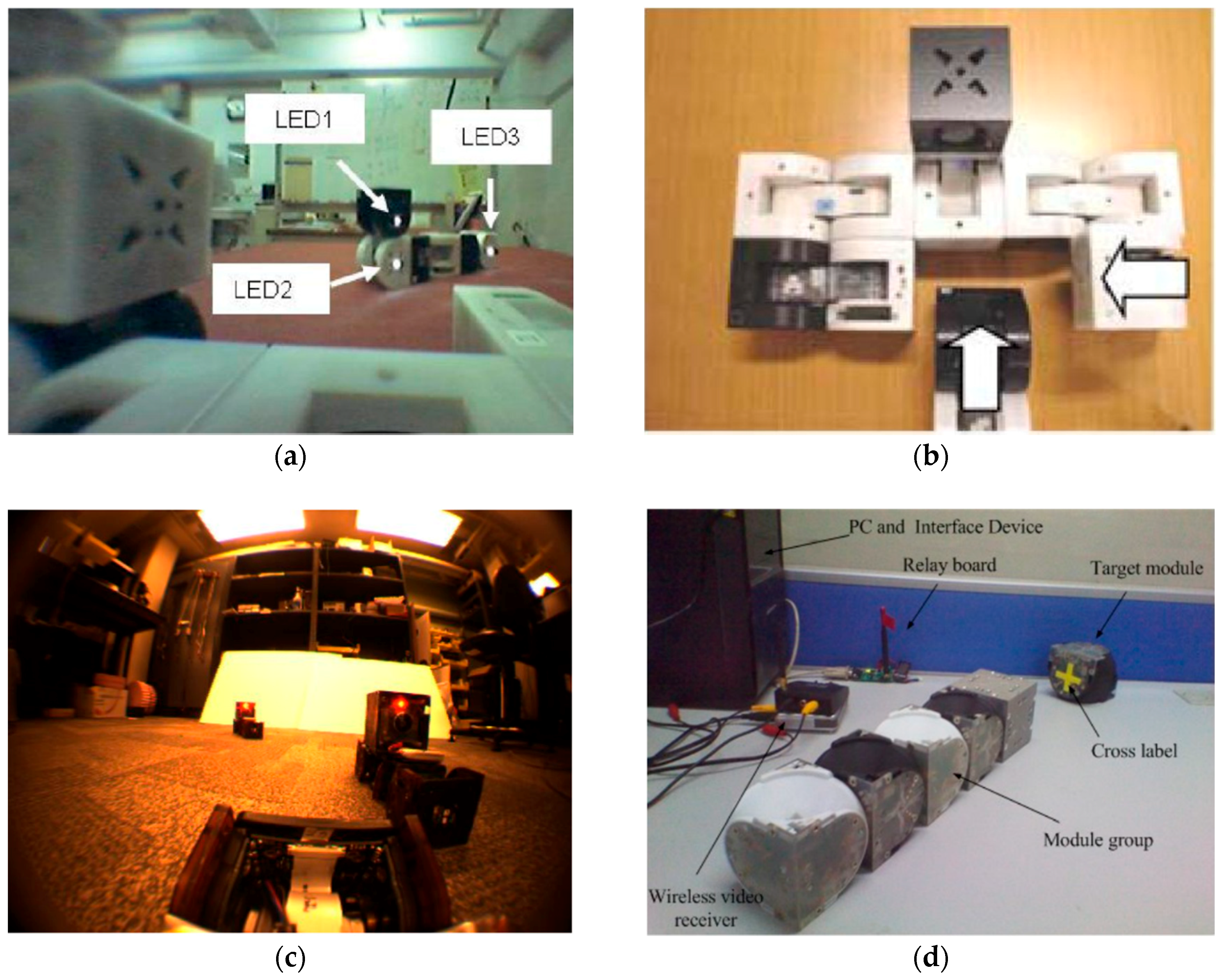
For SMRs that utilize the vision-based methods in autonomous docking, it is important to set proper target features, such as LEDs, special shapes, etc. Not only should the target features make the target robot module easily recognizable, but also it should provide enough information for distance/orientation measurement. Additionally, each docking module should have target features that can provide unique identification.

As showed in

Table 1. Existing self-assembly modular robot (SMR) systems that utilize the vision-based method.

Name	Target Features	Capable of Identifying Different Module	Image Processor (Type)	Location of the Image Processor
M-TRAN	5 white-colored LEDs	No	X86 CPU (PC)	Outside robot
CKBot	LED blink sequences	Yes	PIC18F2680 (MCU)	Camera module of robot
UBot	Cross label on robot	No	X86 CPU (PC)	Outside robot
SambotII	Combination of color-changeable LEDs	Yes	X86 CPU (Edison module)	Inside robot

and Figure 1a, M-TRAN have five LEDs (two on its front face and three on its side face) as its target features. Depending on those LEDs, M-TRAN can determine the distance and orientation of the target-robot group, which consists of three M-TRAN modules and a camera module. However, this method cannot be used to simultaneously identify different robot groups, which means only one docking robot group can be recognized during the docking process. In each M-TRAN system, the captured images are processed by a host PC (personal computer). Because of the limitation in accuracy, the robot group has to form a special configuration to tolerate the docking error (see Figure 1b).

The CKBot can achieve an autonomous docking process after the robot system exploded into three parts, each of which consists of four CKBot modules and one camera module. Some specific LED blink sequences are used as target features for the distance and orientation measurements. In this way, different disassembled parts of the robot system can be identified (see Figure 1c). However, this method costs too much time, because of the large number of images to be processed and the limited computing power of its PIC18F2680 MCU.

For UBot, a yellow cross label is chosen as the target feature (see Figure 1d), by which the distance and orientation between the active and passive docking robot can be determined. Nevertheless, when the distance between the two docking surface is small enough, the UBot will use Hall sensors instead to guide the final docking process. In addition, the UBots are similar to the M-TRANs in two aspects: The images are processed by a host PC; and, different modules cannot be simultaneously distinguished.

1.3. The Present Work

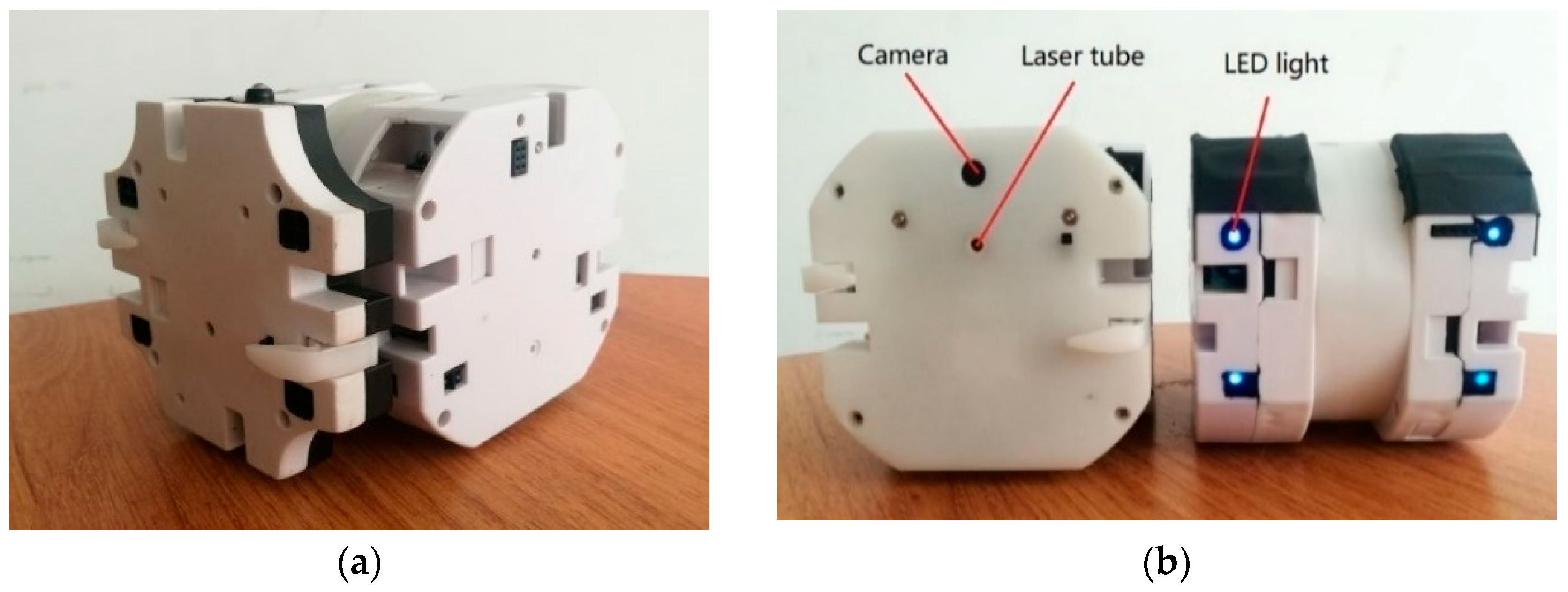
In the present work, a new SMR SambotII is developed based on SambotI [15], a previously-built SMR (Figure 2a), In SambotII (Figure 2b), the original IR-based docking guidance method is replaced by a vision-based method. A laser-camera unit and a LED-camera unit are applied to determine the distance and angle between the two docking surfaces, respectively. Besides, a group of color-changeable LEDs are taken as a novel target feature. With the help of these units and the new target feature, the autonomous docking can be achieved with higher efficiency and accuracy.

An Intel x86 dual-core CPU is applied to improve the computing ability for image processing, information extraction, and other tasks with large computing consumption in the future. Besides, a five-layer hierarchical software architecture is proposed for better programming performances and it is a universal platform for our future research.

Compared with existing SMRs utilizing the vision-based method, the SambotII has three main advantages: (1) The autonomous docking process is more independent, because the whole procedure, including image process and information extraction, is controlled by the SambotII system itself. (2) Apart from distance and orientation measurement, the target feature can be used to identify different modules simultaneously. (3) The docking process is more accurate and efficient, because it costs less than a minute and no extra sensors or procedures are needed to eliminate the docking error.

In the remaining parts, a brief description is given at first for the mechanical structure, electronic system, and software architecture. Then, a detailed introduction is made on the principle of the laser-camera unit, LED-camera unit and docking strategy. Finally, docking experiments are preformed to verify the new docking process.

2. Mechanical Structure of SambotII

As displayed in

Table 2. Main parameters of SambotII.

Content	Parameters
Overall sizes	120 mm × 80 mm × 80 mm
Weight	Approx. 355 g
DOFs	4 (1 neck rotation + 2 wheels + 1 hook)
Connector	A pair of mechanical hooks
Torque of neck	1.3 Nm (max)
Motion method	A pair of wheels
Power source	Inner 7.4V Lithium battery
Battery capacity	Approx. 1200 mAh (8.88 Wh)
Assistant peripherals	Laser tube, LEDs, switches and, etc.
Vision module	HD CMOS camera
Camera resolution	640 × 480 mode (currently used) or 1920 × 1080 mode (maximum resolution)
Wireless system	Wi-Fi 2.4 G/5.8 G + Bluetooth 4.0
Coprocessor	ARM Cortex-M3 STM32
Central Processing Unit	Intel Atom dual-core x86 CPU

, each SambotII is an independent mobile robot containing a control system, a vision module, a driving module, a power module, and a communication system.

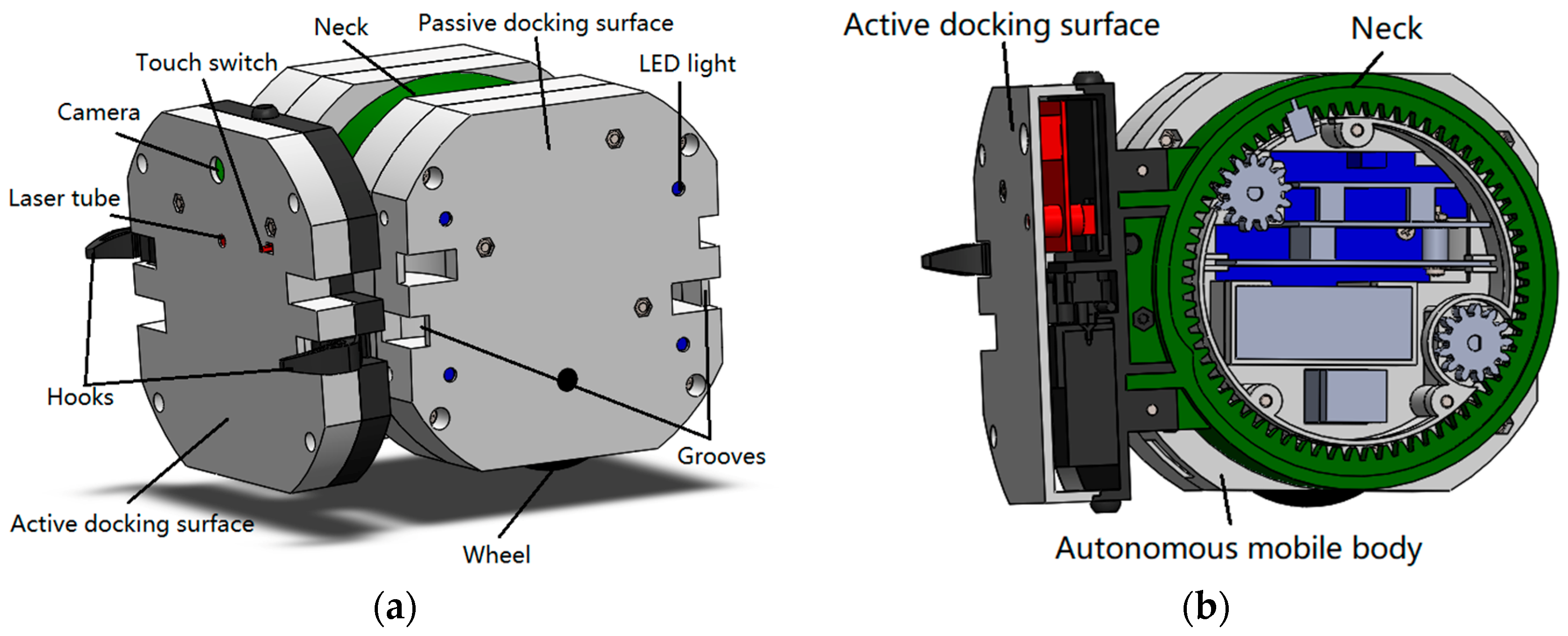
The mechanical structure of SambotII includes an autonomous mobile body and an active docking surface. They are connected by a neck (the green part in Figure 3). Each active docking surface has a pair of hooks.

2.1. Autonomous Mobile Body

The autonomous mobile body of SambotII is a cube with four passive docking surfaces (except for the top and the bottom surfaces). Each passive docking surface contains four RGB LED lights and a pair of grooves. The hooks on the active docking surface of a SambotII robot can stick into the grooves of a passive docking surface of another SambotII robot to form stable mechanical connection between them. The LED lights are used to guide the active docking robot during the self-assembly process. Also, they are used to identify different passive docking surfaces by multiple combinations of colors. In addition, two wheels on the bottom surface of the main body provide mobility for SambotII.

2.2. Active Docking Surface

Actuated by a DC motor, the active docking surface could rotate about the autonomous mobile body by ±90°. It contains a pair of hooks, a touch switch, a camera, and a laser tube. As mentioned above, the hooks are used to form a mechanical connection with a passive docking surfaces of another SambotII. The touch switch is used to confirm whether the two docking surfaces are touched or not. The camera and laser tube are used for distance measurement and docking guidance, and they will be described in detail in the following parts.

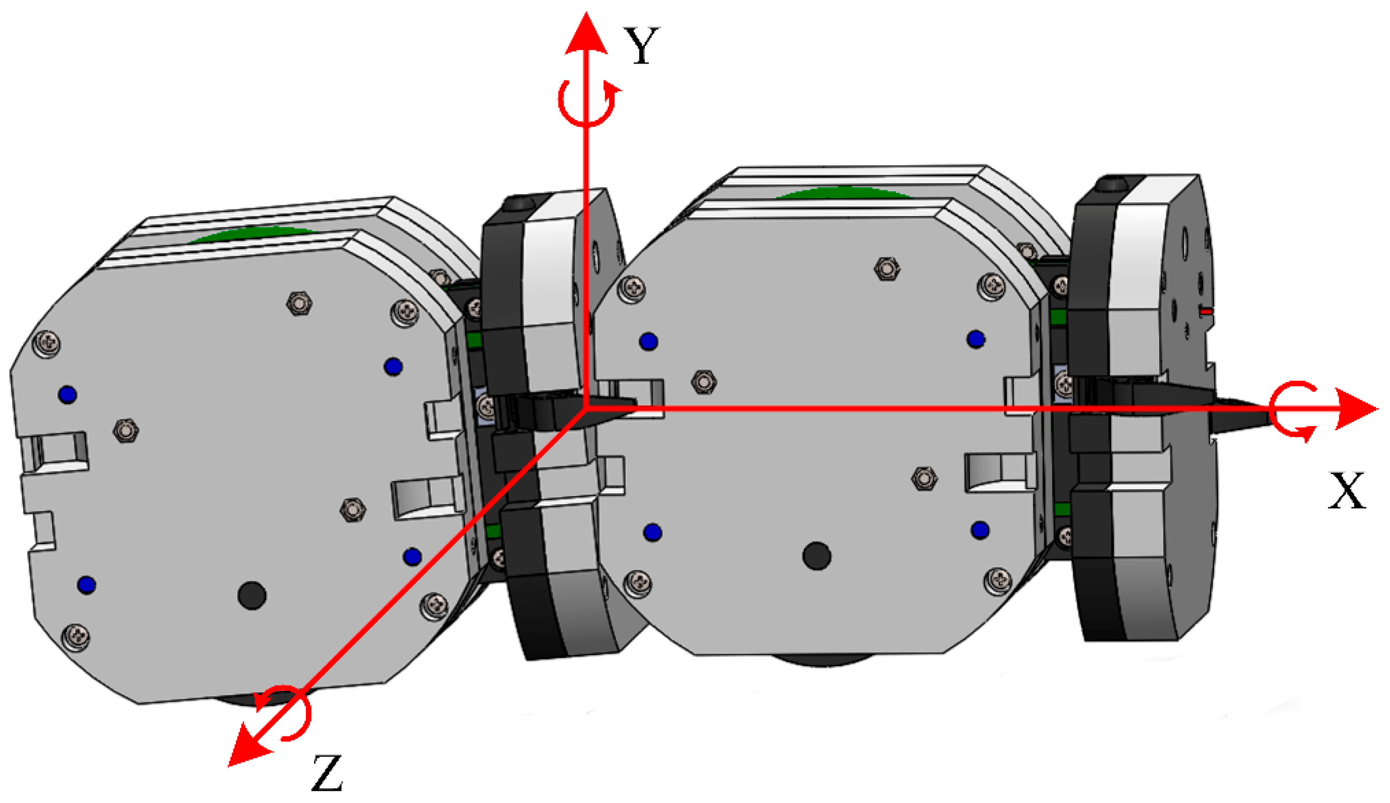
2.3. Permissible Errors of the Docking Mechanism

It is necessary to mention that there are multiple acceptable error ranges during the docking process of two robots (see Figure 4 and

Table 3. The acceptable docking deviation between two SambotIIs.

Direction	Permission Deviation/mm	Direction	Permission Deviation/(°)
Movement along X	13	Rotation around X	$\pm 5$
Movement along Y	$\pm 4.5$	Rotation around Y	10
Movement along Z	$\pm 19.5$	Rotation around Z	$\pm 5$

), which can enhance the success rate of docking. The analysis of permissible errors is given in [16].

3. Information System of SambotII

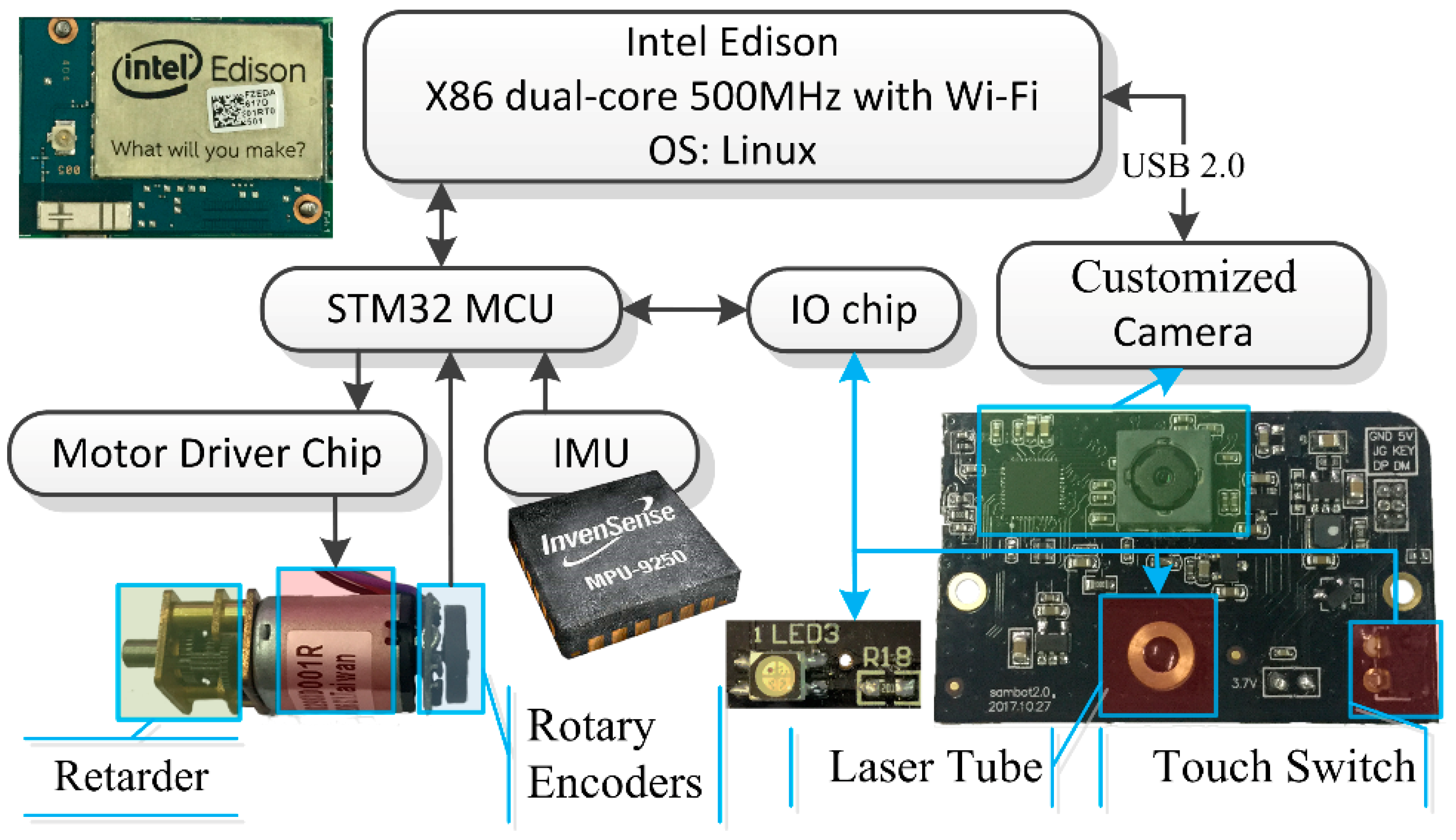
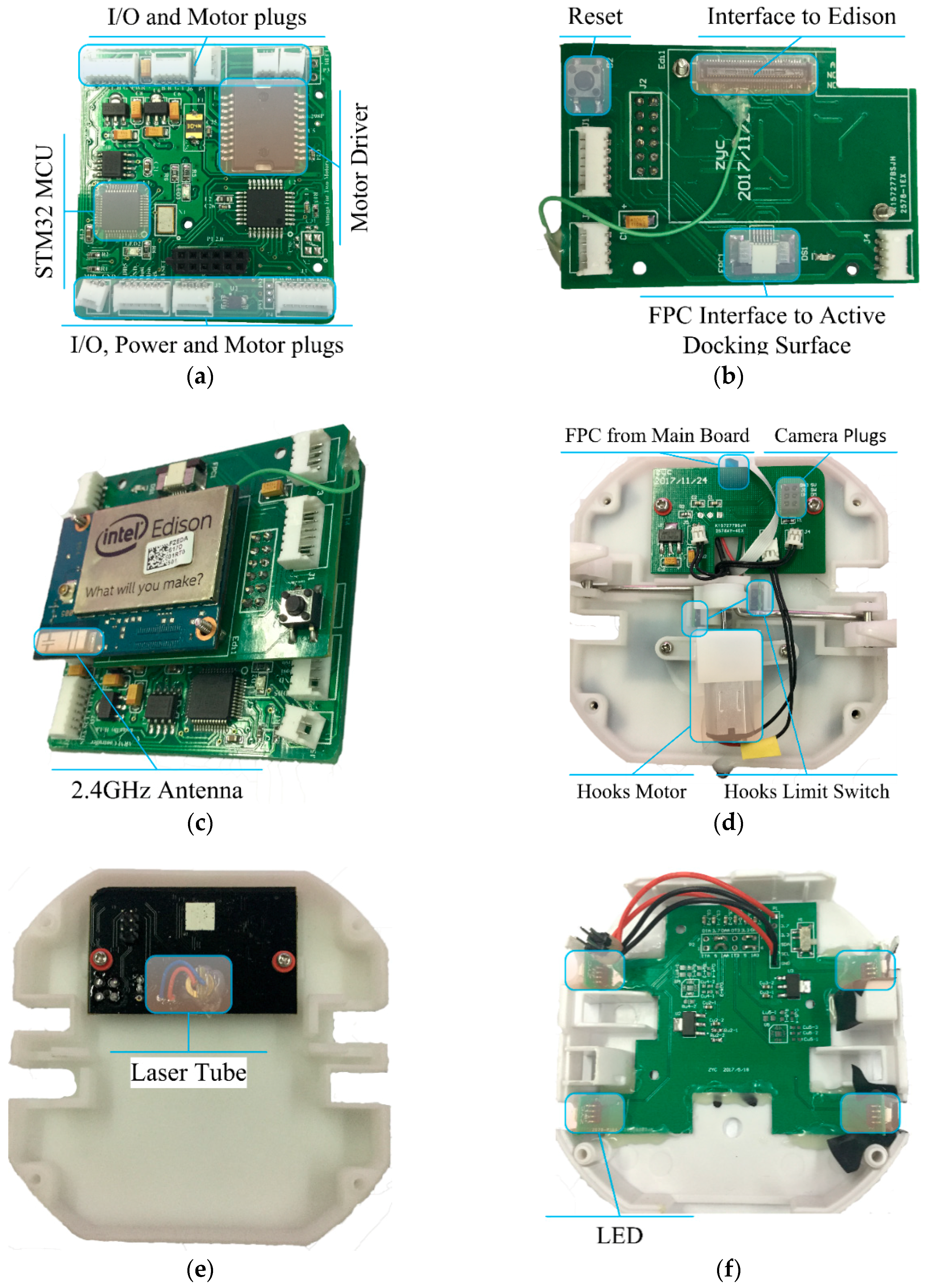
One noticeable improvement of SambotII, as compared with SambotI, is the information system (see Figure 5). The perception, computing, and communication abilities are enhanced by integrating a camera, a MCU (i.e., a microprocessor unit that serves as a coprocessor), a powerful x86 dual-core CPU, and some other sensors into a cell robot. Figure 6 shows the major PCBs (Printed Circuit Board) of SambotII.

The information system consists of three subsystems: The actuator controlling system, the sensor system, and the central processing system.

The actuator controlling system controls motors, which determine the movement and operations of SambotII. The PWM signals are generated by a MCU at first, and then they are transmitted into the driver chip to be amplified. Those amplified analog signals are eventually used to drive the customized motors. Each motor is integrated with a Hall effect rotary encoder, which converts angular velocity into pulse frequency and then feed back into MCU, forming a closed-loop control system. When combining with limit switches, the MCU can open or close the hooks and rotate the neck. By controlling the I/O chip, the MCU can change the colors of LED lights, read the states of switches and turn on or off the laser.

The sensor system includes the encoders, switches, an IMU (Inertial Measurement Unit used to measure orientation and rotation) and a customized HD CMOS camera. Combined with laser tube and LED lights, the sensor system can measure the distance and angle between two docking robots. By identifying the combination of color-changeable LED lights, the robot can locate the specific surface it should connect with during the self-assembly procedure.

The central processing system is a high-density integrated module [17] (see Figure 5) that contains an Intel Atom CPU, a storage, a wireless, etc. (see

Table 4. Features of the Intel Edison CPU module.

Components	Description
Processor	Dual-core, dual-threaded Intel Atom CPU at 500 MHz with 1MB cache. Supporting SIMD SSE2, SSE3, SSE4.1/4.2
RAM memory	1 GB
Storage	4 GB eMMC
Wireless	2.4 and 5 GHz IEEE 802.11a/b/g/n
Bluetooth	BT4.0
USB	USB2.0 OTG
Sizes	35.5 × 25.0 × 3.9 mm

). It supports Linux Operation System (OS) and can run multiple softwares concurrently, capture pictures from the camera through USB, and communicate with other robots through Wi-Fi. Moreover, it is binary compatible with PC.

4. Software Architecture and Task Functions of SambotII

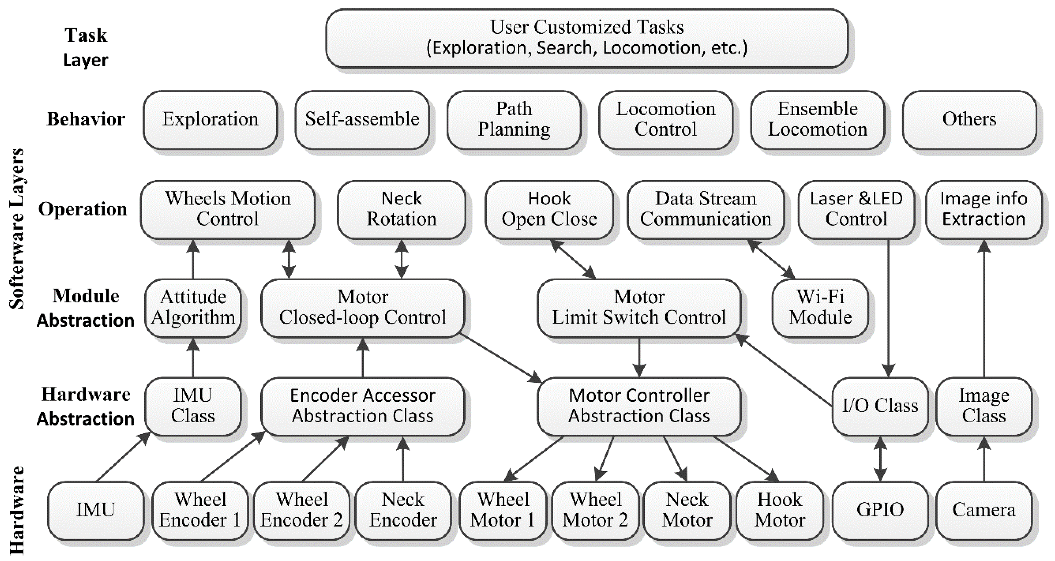
A hierarchical architecture is proposed for the software system. As shown in Figure 7, the hardware and software are decoupled from each other in the architecture. It improves the software reusability and simplifies programming by using the uniform abstract interfaces between different layers and programs.

There are five main layers in the software system: (1) hardware abstract layer; (2) module abstract layer; (3) operation layer; (4) behavior layer; and, (5) task layer. Different layer consists of different blocks, which are designed for particular functions and offer implementation-irrelevant interfaces to upper layers.

The hardware abstract layer acts as an abstract interconnection between the hardware and the software. All the control details of the hardware are hidden in this layer. For instance, the “motor controller abstraction class” controls four motors and offers an interface for upper layer to adjust motor speed. The “encoder accessor abstraction class” processes pulse signals generated by the encoder and converts them into velocity and positional data. The I/O class reads and sets GPIO through I/O chip. The “IMU class” reads the rotation and acceleration data from IMU. These four classes are built in MCU to meet real-time requirements. Besides, the “image class” captures images from the camera by utilizing the OpenCV library in Intel Edison module.

The module abstract layer offers higher level module abstractions by integrating the blocks of the hardware abstract layer into modules. For instance, the “motor closed-loop control class” reads velocity and positional data from the “encoder accessor abstraction class” and sends speed commands to the “motor controller abstraction class”. With the inner control algorithms, it can control speed and position, making it easier for the operation layer to control robot’s motion, and so does the “motor limit control class”. The “attitude algorithm class” reads data from the “IMU class” and calculates the orientation after data filtering and fusion. Finally, the Wi-Fi module is used to establish the wireless network environment for data communication.

The operation layer contains operation blocks, which control the specific operations of the robot. For example, the “wheels motion control block” in the operation layer combines the “motor closed-loop control block” and the “attitude algorithm block”, and so it can control the movement operations of the robot. In this way, we can just focus on designing the behavior and task algorithms, rather than the details of motor driving, control, or wheels movement. Similarly, the blocks, “neck rotation”, “hooks open close”, “laser control”, and “LED control”, are used to control the corresponding operations of the robot, respectively. The “image info extraction block” is designed to extract the useful information we care about from images. Through the “data stream communication block”, robots can coordinate with each other by exchanging information and commands.

The behavior layer is a kind of command-level abstraction designed for executing practical behaviors. A behavior can utilize operation blocks and other behavior blocks when executing. For instance, if the robot needs to move to a certain place, the “locomotion control behavior block” first performs path planning behavior after it receives the goal command, and then it continuously interacts with the “wheels motion control block” until the robot reaches the target position. In the docking behavior, the “Self-assembly block” will invoke the “hooks open close block”, “locomotion block”, “image info extraction block”, and so on. Also, the “exploration block” can achieve information collection and map generation by combing the “locomotion block”, “data stream communication block”, and “image processing block”.

The task layer consists of tasks, the ultimate targets that user wants robots to achieve. Each task can be decomposed into behaviors. For example, if the robots are assigned with a task to find something, they will perform the “exploration behavior” for environmental perception, the “locomotion-control behavior” for movement, as well as the “self-assembly and ensemble locomotion behaviors” for obstacle crossing.

5. Self-Assembly of SambotII

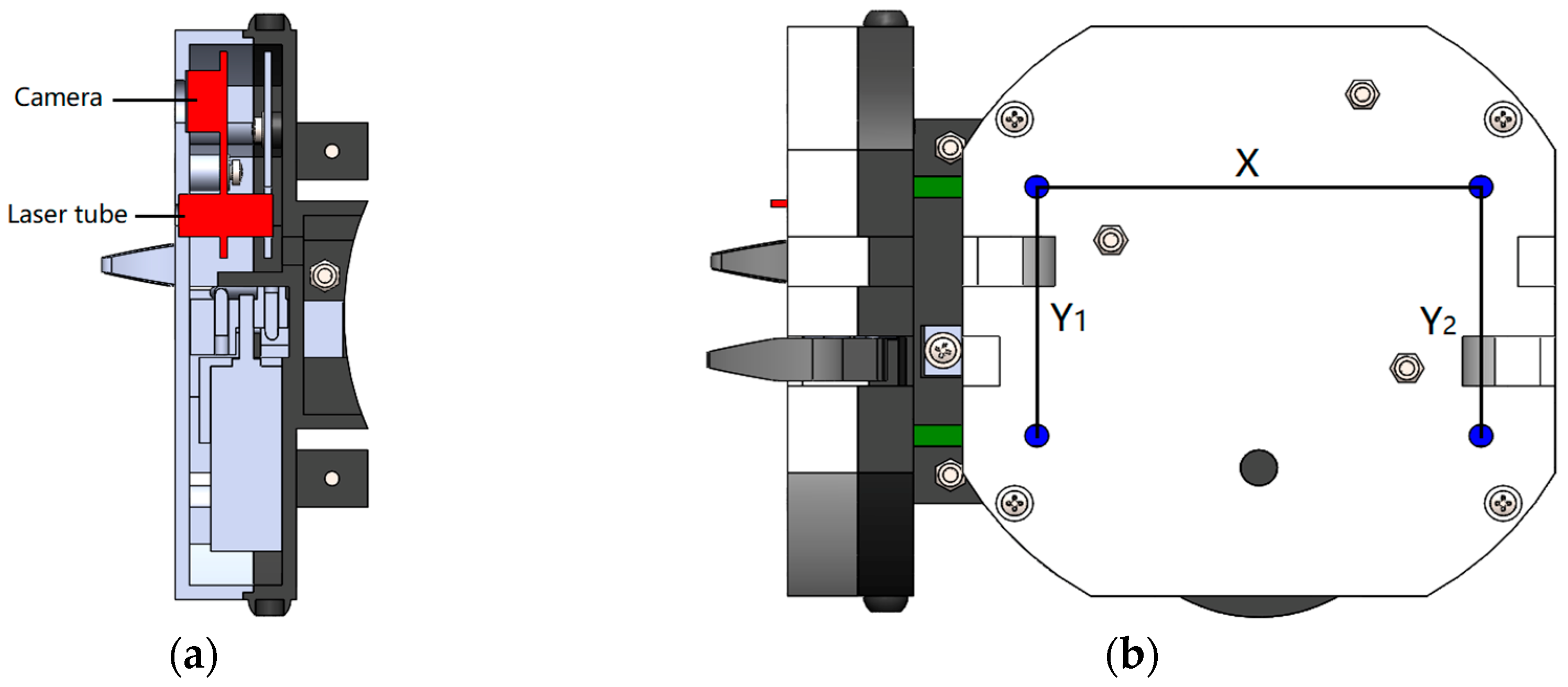
During the self-assembly process of SambotII, it is necessary to obtain the information of distance and angle between the two docking robots. For this purpose, a laser-camera unit and a LED-camera unit are employed to gain the distance and angle, respectively. The position of the camera, laser tube, and LED lights are shown in Figure 8.

5.1. Laser-Camera Unit

As is known, the idea of laser triangulation means the formation of a triangle by using a laser beam, a camera and a targeted point. The laser-camera unit consists of a laser tube and a camera, both of which are installed parallel on the vertical middle line of the active docking surface (see Figure 3a and Figure 8a). 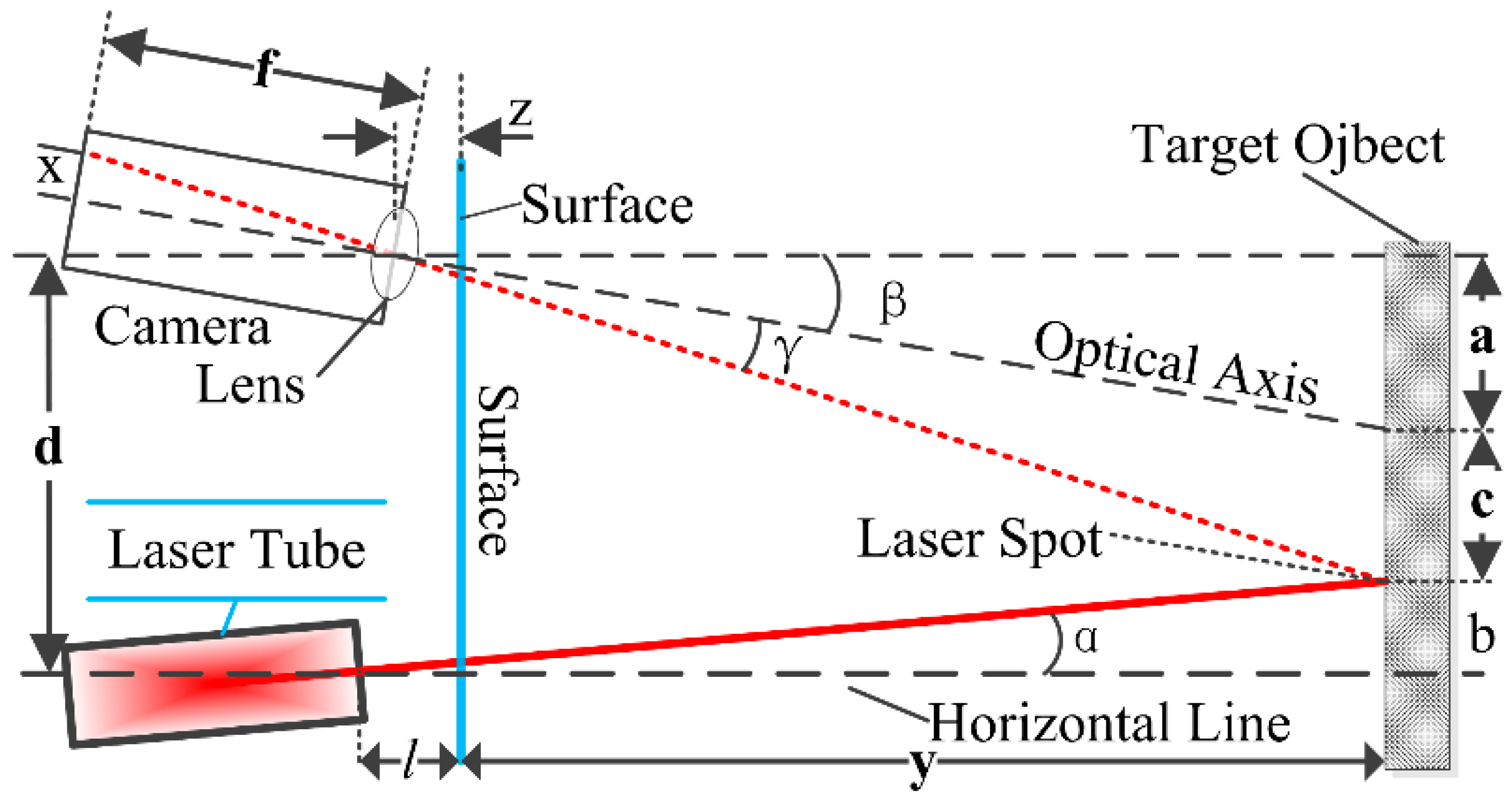Due to the actual machining and installation errors, the optical axes of the camera and laser may be inclined to some extent (see α and β showed in Figure 9). Here, α indicates the angle between the central axis of the laser beam and the horizontal line, while β represents the angle between the camera and the horizontal line. Theoretically speaking, the position of the laser spot that is projected in the camera image (x) changes with the distance between the object and the active docking surface.

In Figure 9, the ‘Surface’ denotes the active docking surface and the right panel refers to a target object. The parameter x stands for the distance between the laser projection spot and the central point of the captured image. The x is calculated by the number of pixels, y denotes the actual distance between the active docking surface and the measured object, and z is the distance between the camera lens and the active docking surface. The parameter d is the vertical distance between the center of camera lens and the emitting point of the laser beam. f represents the focal distance of camera and l is the distance between the laser tube and surface.

According to the principle of similar triangles and the perspective projection theory, one can get:

$$b=\tan \alpha \left(l+y\right)$$

(1)

$$a+c=d-b$$

(2)

$$\tan \left(\gamma +\beta \right)=\frac{a+c}{z+y}=\frac{\left(x+f\tan \beta \right)\sin \left(90°-\beta \right)}{f\frac{1}{\cos \beta }-\left(x+f\tan \beta \right)\cos \left(90°-\beta \right)}$$

(3)

From Formulas (1)–(3), one can obtain:

$$Axy+Bx+Cy+D=0$$

(4)

where

$$A=\cos \beta -\tan \alpha \sin \beta$$

(5)

$$B=z\cos \beta +d\sin \beta -\tan \alpha \sin \beta \cdot l$$

(6)

$$C=f\left[\sin \beta +\tan \alpha \left(\frac{1}{\cos \beta }-\tan \beta \sin \beta \right)\right]$$

(7)

$$D=f\left[\sin \beta \left(z+d\tan \alpha \right)-d\frac{1}{\cos \beta }+l\tan \alpha \left(\frac{1}{\cos \beta }-\tan \beta \sin \beta \right)\right]$$

(8)

Based on Formulas (4)–(8), one can determine the relationship between x and y. The values of coefficients A, B, C, and D can be obtained by using the methods of experimental calibration and the least square estimation algorithm.

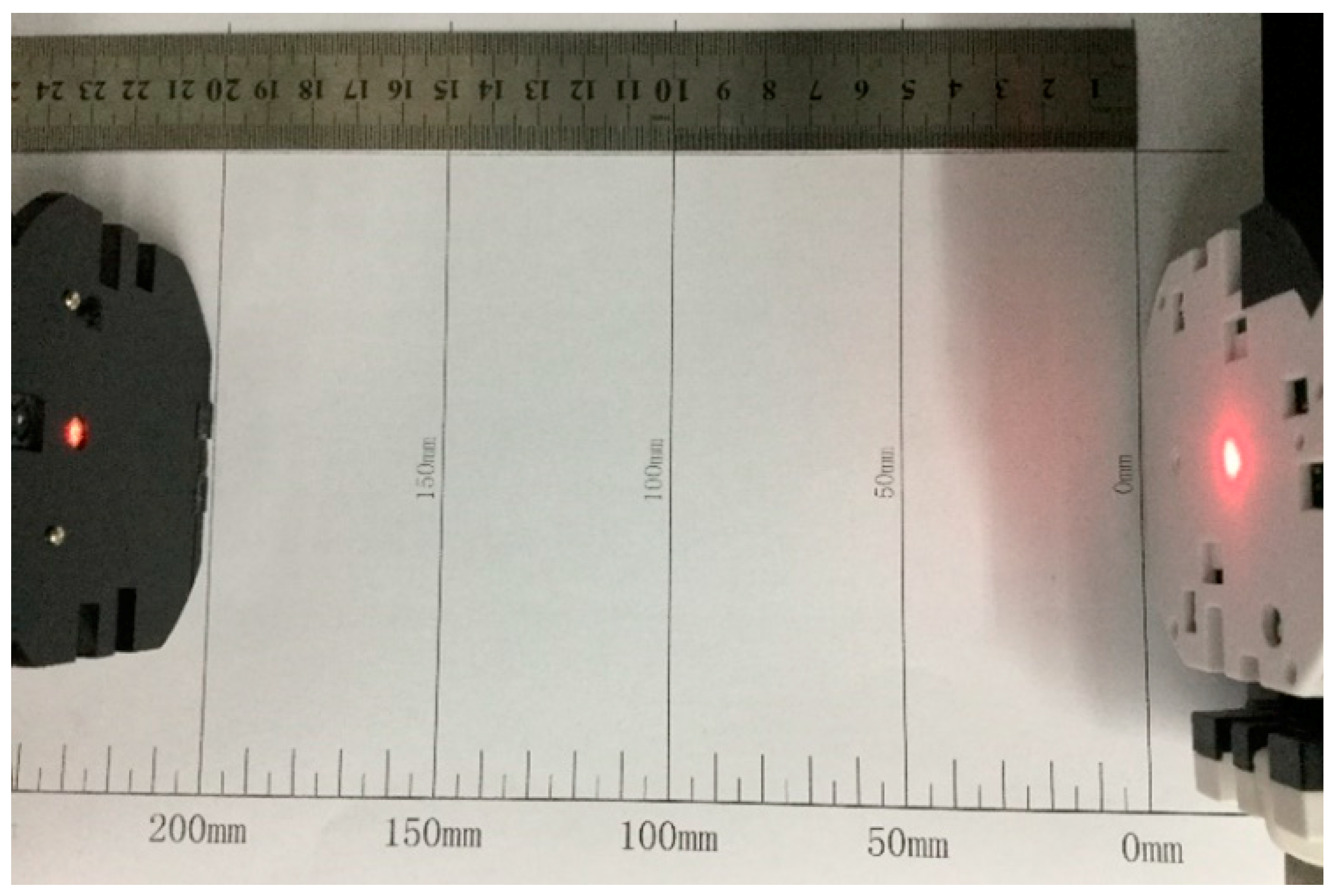
Figure 10 shows the calibration process of the laser-camera unite. The distance between the camera and target is marked as $y_i$ (e.g., In Figure 10 $y_i$ = 0.2 m), and the vertical distance between the laser point and the center of image shown in camera was marked as $x_i$. In the calibration process, n pairs of $x_i$ and $y_i$($1\le i\le n$) can be obtained by putting the camera at different distances from 50 mm to 300 mm for several turns.

The sum of the squared-residual is defined as:

$$S={\displaystyle \sum }_{i=1}^n{\left(A{x}_i{y}_i+B{x}_i+C{y}_i+D\right)}^2$$

(9)

In order to estimate the optimal values of A, B, C and D, S must be minimized. So, the following equations should be simultaneously satisfied:

$$\frac{\partial S}{\partial A}=2\left[A{\displaystyle \sum }_{i=1}^n{\left(x_i{y}_i\right)}^2+B{\displaystyle \sum }_{i=1}^n\left(x_i^2{y}_i\right)+C{\displaystyle \sum }_{i=1}^n\left(x_i{y}_i^2\right)+D{\displaystyle \sum }_{i=1}^n\left(x_i{y}_i\right)\right]=0$$

(10)

$$\frac{\partial S}{\partial B}=0$$

(11)

$$\frac{\partial S}{\partial C}=0$$

(12)

Then, a system of linear equations can be derived, as below:

$$\left[\begin{array}{cccc}{\displaystyle {\displaystyle \sum }_{i=1}^n}{(x_i{y}_i)}^2& {\displaystyle {\displaystyle \sum }_{i=1}^n}(x_i^2{y}_i)& {\displaystyle {\displaystyle \sum }_{i=1}^n}(x_i{y}_i^2)& {\displaystyle {\displaystyle \sum }_{i=1}^n}(x_i{y}_i)\\ {\displaystyle {\displaystyle \sum }_{i=1}^n}(x_i^2{y}_i)& {\displaystyle {\displaystyle \sum }_{i=1}^n}{x}_i^2& {\displaystyle {\displaystyle \sum }_{i=1}^n}(x_i{y}_i)& {\displaystyle {\displaystyle \sum }_{i=1}^n}{x}_i\\ {\displaystyle {\displaystyle \sum }_{i=1}^n}(x_i{y}_i^2)& {\displaystyle {\displaystyle \sum }_{i=1}^n}(x_i{y}_i)& {\displaystyle {\displaystyle \sum }_{i=1}^n}{y}_i^2& {\displaystyle {\displaystyle \sum }_{i=1}^n}{y}_i\end{array}\right]\left[\begin{array}{c}A\\ B\\ C\\ D\end{array}\right]=\mathbf{0}$$

(13)

Formula (13) is a singular matrix equation, so let D = 1. Here, are:

$$\xi ={\left(X^{T}X\right)}^{-1}\left(X^{T}Y\right)$$

(14)

Where Y is a n × 3 matrix with all elements being 1 and ξ and X are defined as:

$$\xi ={\left[\begin{array}{ccc}A& B& C\end{array}\right]}^T$$

(15)

$$X=\left[\begin{array}{ccc}{x}_1{y}_1& x_1& y_1\\ ⋮& ⋮& ⋮\\ x_n{y}_n& x_n& y_n\end{array}\right]$$

(16)

From Formulas (14)–(16), the value of coefficients A, B, and C can be determined. Finally, the relationship between x and y can be expressed as:

$$y=\frac{-D-Bx}{Ax+C}$$

(17)

According to the measurement principle, the accuracy will reduce dramatically with the increasing distance, because the resolution of camera is limited. In actual experiments, it is found that the error is ±5 mm, when the distance between the target and the active docking surface is within 50 cm. If the distance is more than 50 cm and less than 150 cm, the maximum error may reach 15 mm. Under this condition, the value of measured distance is useless. Therefore, the actual docking process should be performed within 50 cm.

5.2. LED-Camera Unit

In order to determine the angle between two docking surfaces, a LED-camera unit is designed and a three-step measurement method is proposed.

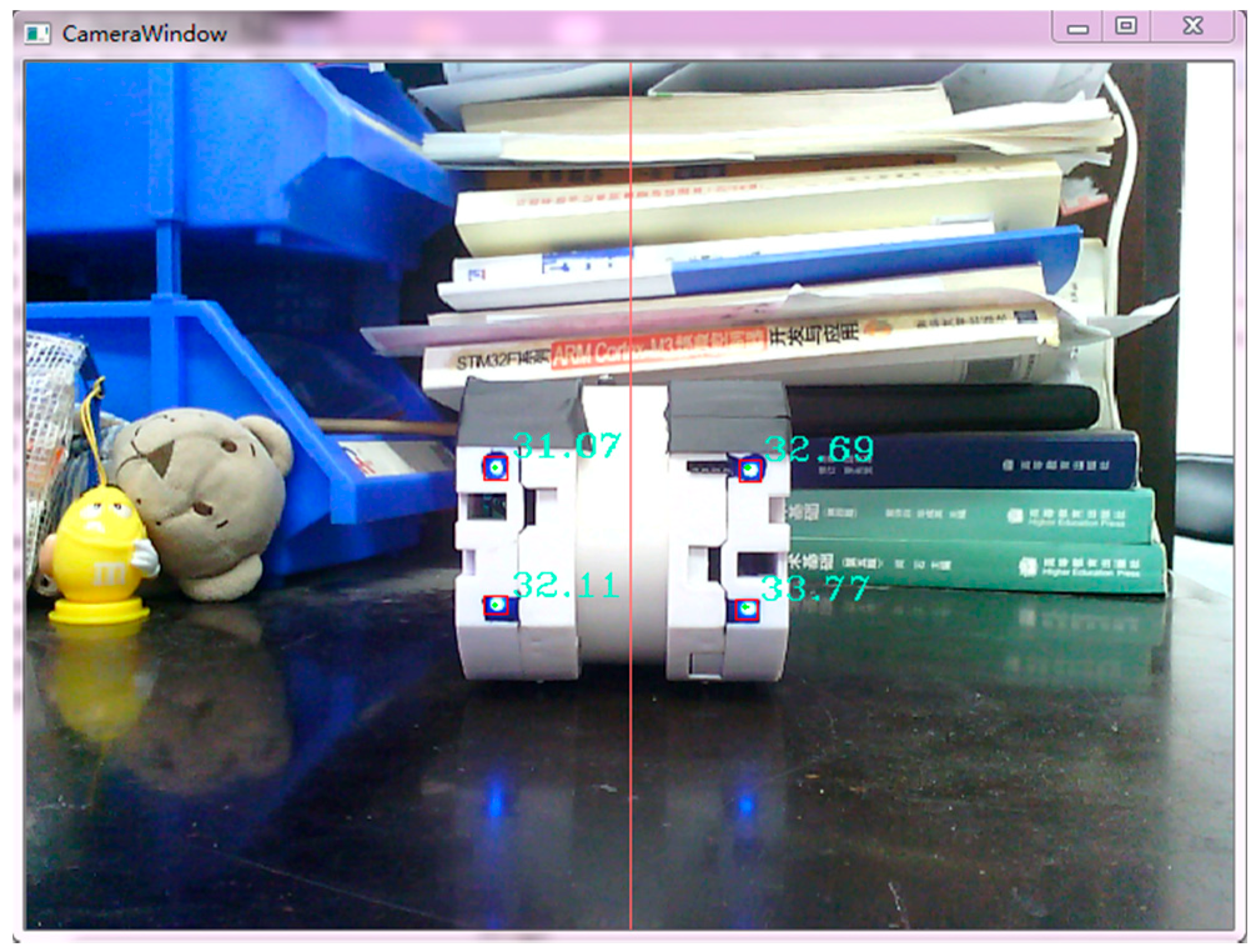
The first step is to determine the relationship between the horizontal distance x of the adjacent LED lights showed in captured image and the actual distance L between the two docking surfaces. The LED identification algorithms can be used to find out the LEDs in complex backgrounds and determine their positions in the image, as shown in Figure 11, where each LED is marked by a red rectangle. Then, one can work out the value of x.

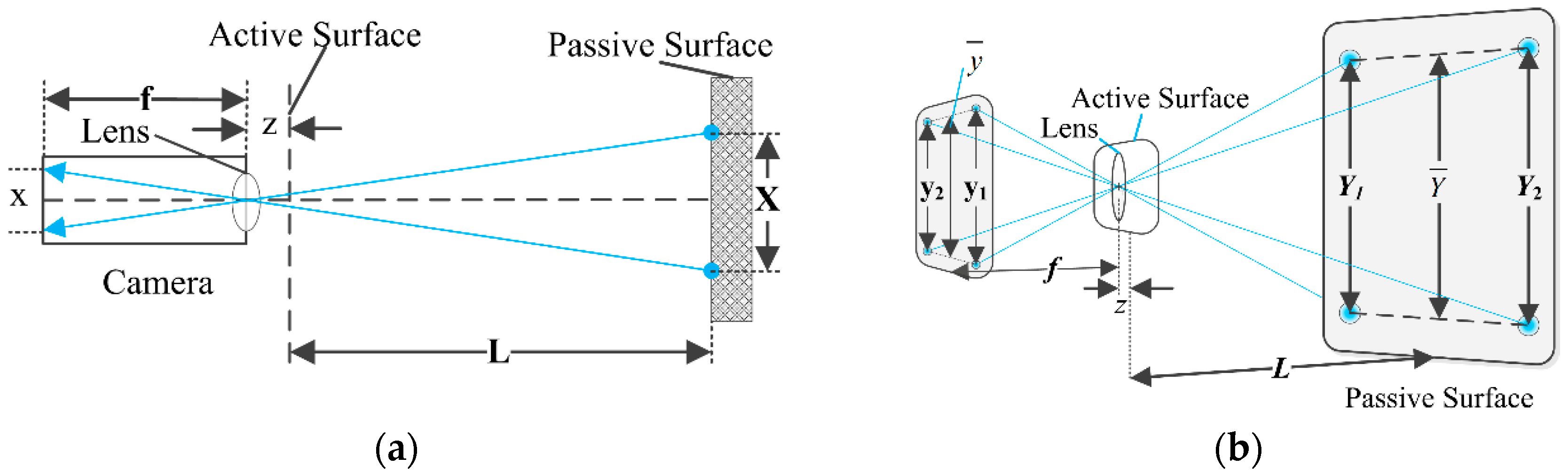
In this step, it is assumed that the two docking surfaces are parallel to each other. The measurement principle is shown in Figure 12a.

In Figure 12, L represents the distance between the passive and active docking surfaces, f denotes the focal distance of the camera, and z is the distance between the camera lens and the active docking surface. In Figure 12a, X is the horizontal distance between the two upper adjacent LED lights on the passive docking surface (also see Figure 8b), and x is the distance calculated from the pixel length that X showed in camera image

According to the principles of similar triangles and perspective projection, one can get:

$$\frac{x}{f}=\frac{X}{L+z}$$

(18)

It can be rewritten as:

$$\left(L+B_1\right)x+D_1=0$$

(19)

Where:

$$B_1=z, D_1=-fX$$

(20)

Similar to the case of laser-camera unit, the two unknown coefficients B and D can be determined by experimental calibration. From Formula (19), x can be expressed as:

$$x=\frac{-D_1}{L+B_1}$$

(21)

The second step is to determine the average vertical distance of the two adjacent LED lights shown in the image at distance L. Here, L is obtained by the LED-camera unit rather than the laser-camera unit. The laser-camera unit can obtain the distance between the camera and the laser spot, however, the distance between the camera and the horizontal center of LEDs (middle of $Y_1$ and $Y_2$) is required. It is hard to assure that the laser spot just locates at the center of LEDs. Thus, if the distance that is obtained by laser is used, it may cause unpredictable error in the result of angle measurement.

As shown in Figure 12b, $Y_1$ and $Y_2$ are the vertical distances of the adjacent LED lights and $\overline{Y}$ is their average value, i.e., $\overline{Y}=\left(Y_1+Y_2\right)/2$. While, $y_1$ and $y_2$ are the images of $Y_1$ and $Y_2$ projected in the camera. The average value of $y_1$ and $y_2$ is $\overline{y}$, i.e., $\overline{y}=\left(y_1+y_2\right)/2$.

Similarly, one can get:

$$\frac{\overline{y}}{f}=\frac{\overline{Y}}{L+z}$$

(22)

It can be rewritten as:

$$\left(L+B_2\right)\overline{y}+D_2=0$$

(23)

where

$$B_2=z, D_2=-f\overline{Y}$$

(24)

Using the same calibration method, one can obtain the relationship between $\overline{y}$ and L as:

$$L=\frac{-D_2-B_2\overline{y}}{\overline{y}}$$

(25)

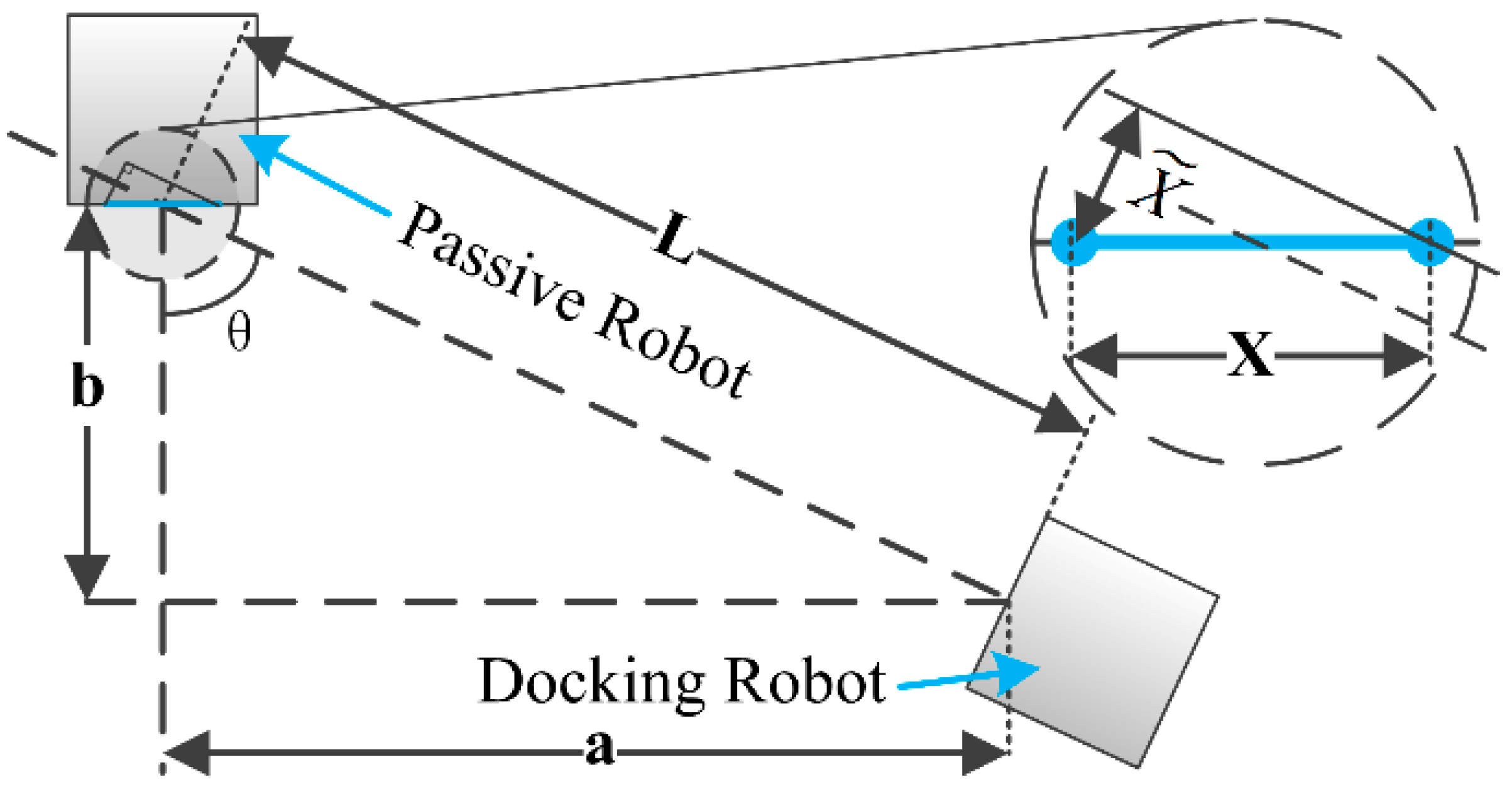
The last step is to determine the angle $\mathsf{\theta }$ between the two docking surfaces. As shown in Figure 13, the two docking surfaces are not parallel to each other in a practical situation. Therefore, the horizontal distance X shown in the image is actually its projection ($\tilde{X}$) in the direction of the active docking surface.

From Figure 13, it can be obtained that:

$$\tilde{X}=X\cos \theta$$

(26)

When considering the distance showed in the captured image, one has:

$$\tilde{x}=x\cos \theta$$

(27)

Contrarily, the average vertical distance y only depends on the distance L between the two docking surfaces and it is not affected by $\theta$.

By combining Formulas (21), (25), and (27), angle $\theta$ could be expressed as:

$$\theta ={cos}^{-1}\left\{\frac{\tilde{x}\left[\left(B_1-B_2\right)\overline{y}-D_2\right]}{-D_1\overline{y}}\right\}$$

(28)

5.3. Experimental Verification of the Angle Measurement Method

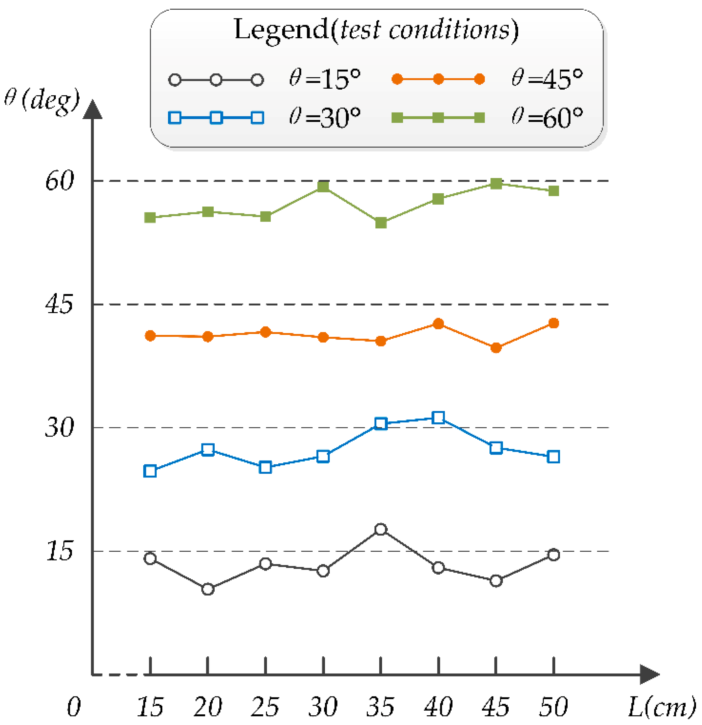
When the angle between two docking surfaces is too large, the adjacent LED lights in the same horizontal surface will become too close to be identified in the image. Thus, four group of data are measured at the angles of 15°, 30°, 45°, and 60°. When the distance between two docking surfaces are too small, the camera cannot capture all of the LED lights. When the distance is too far, the measurement accuracy will reduce dramatically because of the limited resolution of the camera. Therefore, the distance is restricted between 15–50 cm in the angle measurement experiments and its variation step is prescribed as 5 cm. Based on our previous work [18] and the additional supplementary experiment, the measurement results of the angle θ are shown in Figure 14.

From Figure 14, it is seen that the maximum angle error approaches 6°. Except for few data, the overall measurement results are smaller than the actual angle. The error mainly comes from two aspects:

• The error of Formula (21) and (25).
• The error caused by the LED identification algorithm, because the point that is found by the algorithm may not be the center of the LEDs.

Because the mechanical structure of SambotII allows a range of measurement error in the docking process and the maximum error of angle measurement is in that range, the angle information that was obtained by the present LED algorithm can be used in the docking process.

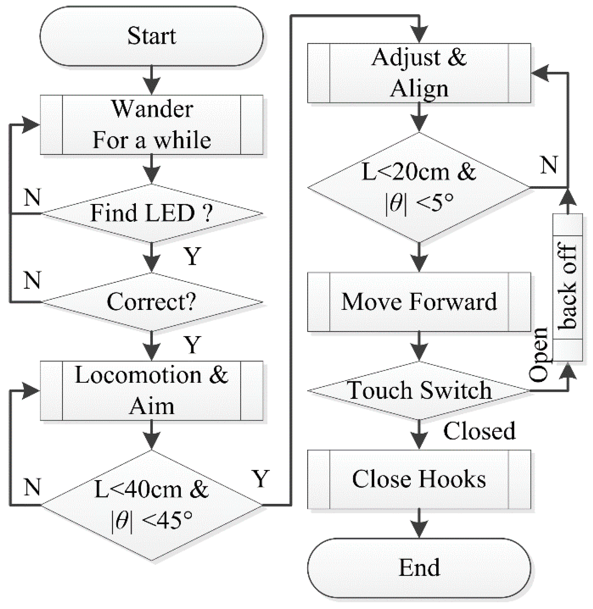
5.4. Outlines of the Docking Strategy

The docking procedure (see Figure 15) is divided into three phases:

• wandering and searching phase;
• position and angle adjustment phase; and,
• docking phase

5.4.1. Wandering and Searching Phase

In this step, the active robot wanders under a certain strategy to explore and search for the correct passive docking surface whose LED lights formed a specific pattern. After finding the target passive docking surface, the robot will enter the next phase.

5.4.2. Position and Angle Adjustment Phase

Because the active robot just move forward directly to complete the docking without extra measurement in the third phase, it should make position and angle adjustment in this step so as to assure that the distance and angle are within specific ranges.

During this phase, a series of adjusting movements need to be performed. In each adjusting movement, the active robot rotates at first to adjust its orientation and then moves forward to adjust its position, because SambotII is a differential wheeled robot. After each adjusting movement, it has to rotate again to face the passive docking surface to check if the specific tolerance condition has been met. Each move-and-check operation generally costs much time. In order to enhance the efficiency, this procedure is further divided into two steps: the rough aiming step and the accurate alignment step.

In the rough aiming step (Locomotion & Aim), the active robot moves a relatively larger distance in each adjusting movement under a loose tolerance condition: L (distance) < 40 cm and θ (deviation degree) < 45°. When this condition is met, the active robot will stop in front of the passive docking surface and face it.

The laser-camera unit has its best performance when L < 40 cm and LED-camera unit has better accuracy when θ < 45°. That is why L < 40 cm and θ < 45° is chosen as the finish condition of this phase.

In the accurate alignment step (Adjust & Align), robot moves a smaller distance in each adjusting movement under a strict tolerance condition: L < 20 and θ < 5°. This condition ensures that the robot can just move forward for docking without check L and θ for a second time, due to the permissible errors of docking mechanism.

The laser-camera is used to get distance during the whole phase, because it is more accurate than the LED-camera. Moreover, when the four LEDs are too far or the angle θ is too large, LEDs may not be clearly recognized for measuring.

5.4.3. Docking Phase

In this phase, the robot opens its hooks and moves forward until it contacts the passive docking surface (when the touch switch is triggered). Then, it closes its hooks to form mechanical connection with the passive docking surface. If failed, it will move backward and restart the position and angle adjustment phase.

6. Docking Experiments

In this section, docking experiments are performed between two robots to verify the entire hardware and software system.

Before the final structure was fixed, two prototypes (see Figure 16) of SambotII are built by adding the camera, laser tube, LED lights, and other components into SambotI. Due to the limitation of size, the hooks in the active docking surface are removed from these prototypes. The coincidence degree of the two docking surfaces is chosen as the evaluation index. In the final structure of SambotII, after the customized camera has been delivered, the hooks are equipped (as shown in Figure 2b).

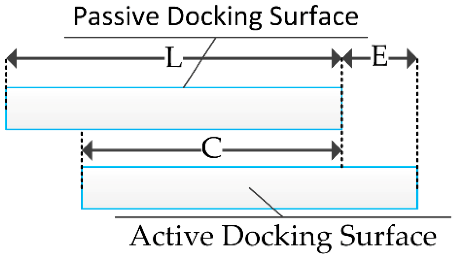
In Figure 17, L = 80 mm is the width of each surface, C is the coincident width of the two surfaces and E is the docking error. The coincidence degree $\eta$ is defined as $\mathsf{\eta }=\left(C/L\right)\times 100\%$. As shown in Table 2, the permission deviation along the Z axis is $\pm 19.5$ mm. Thus, when E is less than 19.5 mm or $\mathsf{\eta }\ge \left[\left(L-19.5mm\right)/L\right]\times 100\%\approx 75\%$, the docking process can be regarded as successful.

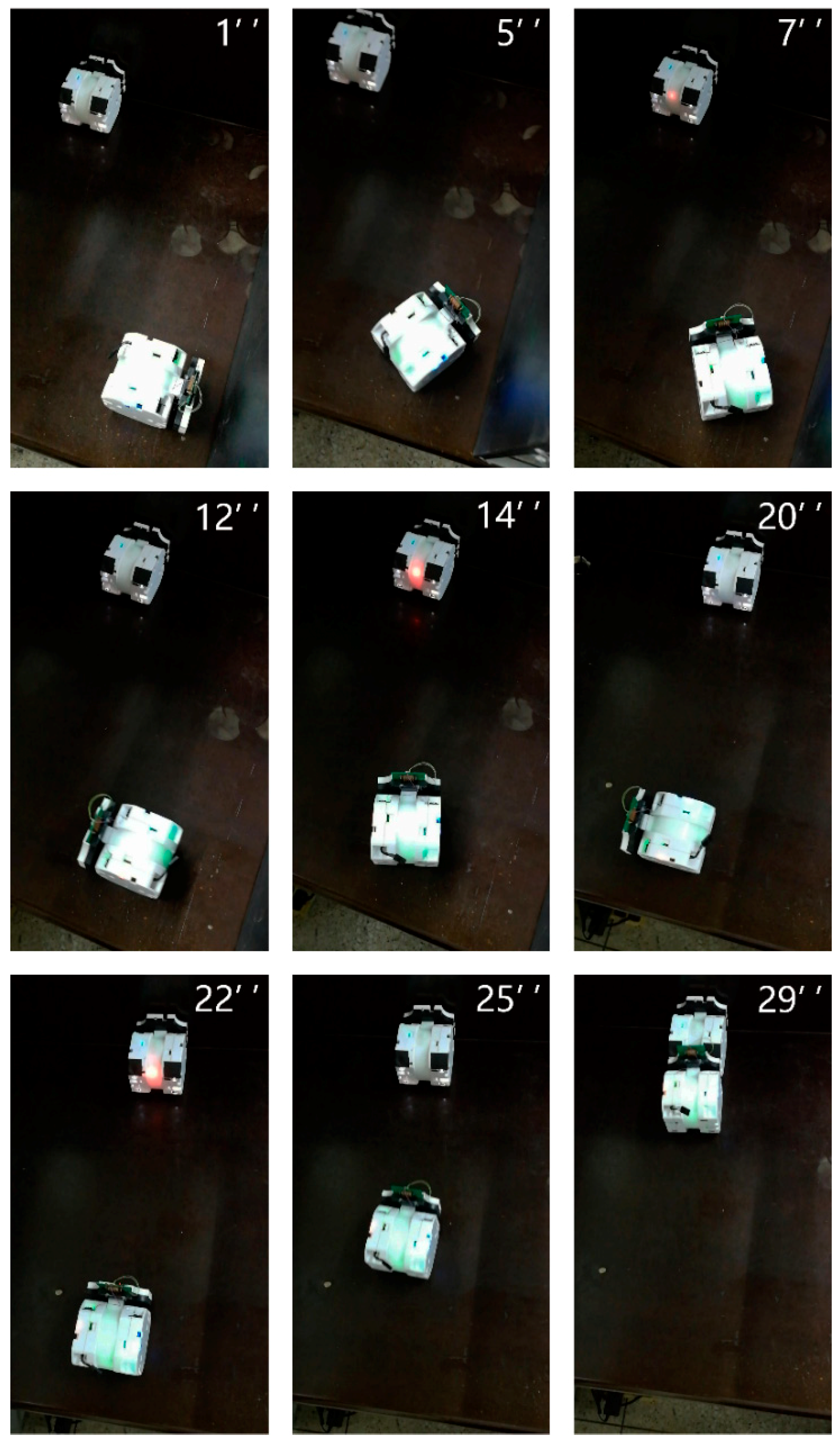
The experiment was carried out on a 60 × 60 cm platform with an enclosure being 40 cm high. Because the enclosure surface is rough, the reflection of light is so weak that the recognition of the laser and LED lights cannot be affected. Because only two robots are applied in the experiments, only the LEDs on one passive docking surfaces are turned on.

The passive robot is placed on one side of the platform and stay still, while the active docking robot is placed on the other side. The docking process is repeated 10 times to evaluate the success rate of the first docking. In each time, if the active robots misses the passive docking surface, the docking process will end, and this experiment is then counted as a failure.

Experiment indicate that the success rate of the first docking is approximately 80%. Thus, the feasibility and validity of the docking algorithm is verified. The experimental results are shown in

Table 5. Result of autonomous docking experiment.

Coincidence Degree	Times
0~64%	1
65~74%	1
75~84%	1
85~94%	4
95~100%	3

[18].

There are two failed dockings in the experiments. One failure occurs due to compound errors. When the accurate alignment step ends, the angle that was calculated by the active robot is less than 5°, but the actual angle might be 6° or 7°. Besides, the speed difference between the two wheels may also lead to angle error. Influenced by these two errors, the final coincidence degree is between 65% and 75%. Another failure may be caused by incorrect LED recognition. When the accurate alignment step ends, the angle between the two robots exceeds the expected value. So, the active robot misses the passive docking surface finally.

The failure caused by errors are inevitable. They can be reduced by improving the measurement accuracy and decreasing the speed difference between the two wheels. The failure cause by LED misrecognition may occur of the light reflected by LED is incorrectly identified as a LED’s light. So, the algorithm should be further optimized to deal with the problem of reflection.

When compared with SambotI, SambotII has higher efficiency and a larger range (it is 50 cm, but for SambotI it is just 20 cm).

7. Conclusions and Future Works

A new self-assembly modular robot (SambotII) is developed in this manuscript. It is an upgraded version of SambotI. The original electronic system is redesigned. An Intel x86 CPU, a memory, a storage, a Wi-Fi module, a camera, a laser tube, and LEDs are integrated into robot for the purpose of improving the computing performance, the communication ability, and the perception capability. Meanwhile, a five-layer hierarchical software architecture is proposed and thus the reliability and reusability of programs are enhanced. By using this architecture, a large application program can be well organized and built efficiently.

Moreover, a laser-camera unit and a LED-camera unit are employed to perform distance and angle measurements, respectively. Besides, by identifying different color combinations of LED-lights, the active robot can find the specific passive docking surface clearly and precisely so that the traditional random try is effectively avoided. Finally, two prototype SambotII robots are used to perform docking experiments, by which the effectiveness of the entire system and docking strategy have been verified.

In general, SambotII can serve as a fundamental platform for the further research of swarm and modular robots. In the future, three major aspects of work can be done for further improvement:

• Hardware optimization, including the increase of battery capacity, the enhancement of the motor’s torque, the improvement of the LEDs’ brightness, the addition of a rotational DOF, the addition of a FPGA chip in robot, and etc.
• Optimization of the LED-identification algorithms so as to improve the angle measurement accuracy.
• Enhancement of the software functions in behavior layer, such as the exploring and path planning.