Parameter Determination of a Minimal Model for Brake Squeal

Abstract

In the research into the mechanism of brake squeal, minimal models with two degrees of freedom (DoFs) are widely used. Compared with the finite element method, the minimal model is more concise and efficient, making it easier to analyze the effect of parameters. However, how to accurately determine its kinetic parameters is rarely reported in the literature. In this paper, firstly, the finite element model of a disc brake is established and the complex eigenvalue analysis (CEA) is carried out to obtain unstable modes of the brake. Then, an unstable mode with seven nodal diameters predicted by CEA is taken as an example to establish the 2-DoF model. In order that the natural frequency, Hopf bifurcation point and real parts of eigenvalues of the minimal model coincide with that of the unstable mode with seven nodal diameters, the response surface method (RSM) is applied to determine the kinetic parameters of the minimal model. Finally, the parameter-optimized minimal model is achieved. Furthermore, the negative slope of friction-velocity characteristic is introduced into the model, and transient analysis (TA) is used to study the effect of braking velocity on stability of the brake system. The results show that the brake system becomes unstable when braking velocity is lower than a critical value. The lower the velocity is, the worse the stability appears, and the higher the brake squeal propensity is.

1. Introduction

Squeal noise of brake system is one of the difficult problems that need to be solved by automobile manufacturers. It is generally believed that the disc brake squeal is self-excited vibrations induced by friction forces. However, for the mechanisms of self-excited vibrations, the existing literatures proposed a different hypothesis. The first type of literaturesholds that the variation characteristics of the friction coefficient lead to squeal instability, including mechanisms like stick-slip [1,2,3] and negative friction-velocity relationship [4,5]. Nevertheless, the stick-slip mechanism is not sufficient to explain the occurrence of the squeal [6]. As pointed out by Ouyang et al. [5], stick-slip occurs only at low speeds of a mass driven across a dry surface, while at a sufficiently high speed the mass will be permanently sliding. This proves that the instability of brake discs can be induced by a negative slope of friction-velocity characteristic even without stick-slip motion. The second type of literature indicates that self-excited vibrations can be induced even at a constant friction coefficient, and demonstrates that the generation of squeal is related to the dynamics of the geometric structure [7,8]. The sprag-slip model introduced in early studies by Spurr [7] illustrates the mechanism of squeal in terms of structural geometry, which means that tribological characteristics should not be considered as the only reason for squeal instability [9]. Later, many scholars confirmed the existence of mode-coupling phenomenon [10,11,12,13] in brake squeal. Hoffman et al. [11] found that when the friction coefficient is greater than a critical value, namely the Hopf bifurcation point, the oscillation frequencies of two structural modes gradually come closer until they coalesce into a pair of an unstable mode and a stable mode. It is clear that mode coupling explains the squeal phenomenon under a constant friction coefficient instead of a variable friction coefficient. In fact, when mode coupling occurs, the system not only generates unstable oscillations, but simultaneously accompanied by a notable nonlinear variation of friction coefficient. This has an important effect on the dynamic response of the system. Therefore, the stability analysis in this paper is based on the combination of mode coupling and negative slope of friction-velocity characteristics.

The modeling method for brake squeal generally includes two categories. One category is to establish the finite element model of brake, then complex eigenvalue analysis (CEA) or transient analysis (TA) is performed for the finite element model [14,15,16]. Ouyang et al. [17] and Kinkaid et al. [18] give a detailed summary of the application of CEA and TA in the study of brake squeal. The other category to investigate squeal is based on minimal models such as the abstract 2-DoF model. Hoffman et al. [11] proposed a 2-DoF model to explain self-excited vibrations induced by mode-coupling mechanism. Shin et al. [19] adopted a 2-DoF model containing lumped masses representing the disc and the pad respectively, through which the effect of negative slope of friction-velocity characteristics on the oscillation instability was investigated. Popp et al. [20] considered the torsional mode of the brake disc in their 2-DoF model. Later, based on the three models above, Wagner [21] put forward a 2-DoF model that further considers vibration of the disc as a rotating elastic plate, so as to associate easily with real disk brake [22]. However, the aforementioned literatures have not given detail descriptions about parameters determination method and its process of the model, and the stability of the model depends greatly on the value of parameters.

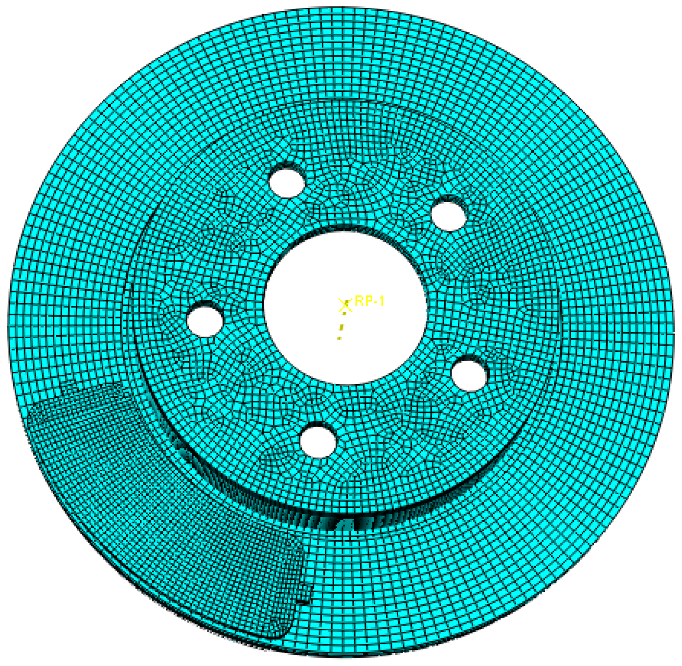
Since brake components are geometrically complex and are essentially continuous media with infinite DoFs, it is appropriate to use the finite element method with less model simplification and a large number of DoFs [17]. The CEA of the finite element method can simultaneously obtain several unstable modes, but it is limited by underestimate or overestimate error due to a linearization assumption [23]. Compared with eigenvalue computation, the TA of the finite element method can achieve the dynamic response of components with nonlinear effects included, such as nonlinearity of friction, contact pressure, and lifting off of the pad (e.g., contact separation between the two sliding surfaces), which are referred to as deterministic chaos by Oberst et al. [24]. So additional unstable modes may be detected while CEA fails. However, it is not conducive to extensive parameter designs because of excessive time consumption [25], so its engineering application is limited. In contrast with a full-scale brake finite element model, the 2-DoF minimal model is of high efficiency during stability analysis owing to its fewer DoFs, although it is a simplification, and can consider only a certain order mode. It is helpful to analyze the effect of key parameters on brake squeal, and to reveal the squeal mechanism [19]. Nevertheless, the parameters in the model are difficult to determine.

Therefore, this paper aims to explore a more accurate method for parameter determination of the 2-DoF minimal model, so as to make up for the shortcomings of existing literatures. The response surface method (RSM) is applied in the parameter determination. Then, TA is performed for the parameter-optimized minimal model to discuss the effect of braking velocity on squeal stability. The results demonstrate that the squeal is more prone to occur under relatively low velocity.

2. Materials and Methods

2.1. Finite Element Analysis of Brake Squeal

As shown in Figure 1, a simple finite element brake model with a disc, two pads and two back plates is established in ABAQUS.

Table 1. Material properties of brake components.

	Disc	Back Plate	Pad
Young’s Modulus (MPa)	135,000	182,000	D1111	5940	D1133	980	D1212	2590
			D1122	760	D2233	980	D1313	1180
			D2222	5940	D3333	2270	D2323	1180
Density (t/mm3)	${7.2\times 10}^{-9}$	${7.8\times 10}^{-9}$	${2.51\times 10}^{-9}$
Poisson’s ratio	0.27	0.3

shows the material properties of the three brake components [26], where the brake pads are made of orthotropic material, and its nine elastic constants are given. The back plates are constrained using YASYMM boundary condition, namely, constraining the X, Z direction of the displacement and rotation around the Y axis, and the bolt holes on the disc are constrained with PINNED boundary condition, namely, constraining the X, Y, Z direction of the displacement. A uniform pressure of 1 MPa is applied to the back plates to simulate the actual braking hydraulic load.

The complex modal analysis of the model is carried out, and the rotation effect is applied to the brake disc in the input file. Finally, eigenvalues of the first 55 complex modes of the model are extracted. Figure 2 shows the frequencies and real parts of the eigenvalues of unstable modes.

It can be seen from Figure 2 that the brake system has several unstable modes which may lead to brake squeal. With the increase of the friction coefficient, the number of unstable modes increases; therefore, the propensity of brake squeal increases. For the friction coefficient $\mu =0.9$, 8 unstable modes are predicted in the system. Their frequencies are 4060.2 Hz, 5525.5 Hz, 7213.0 Hz, 8429.0 Hz, 9042.1 Hz, 11,056 Hz, 11,198 Hz and 11,496 Hz respectively.

For instance, the unstable mode with seven node diameters is shown in Figure 3. Figure 4a shows the evolution of real parts of the mode with respect to the friction coefficient from 0.2 to 0.9, namely the Hopf bifurcation diagram. The bifurcation point of this mode is observed for ${\mu }_0=0.4$. For friction coefficients greater than 0.4, the real parts of this mode are positive, which signifies an unstable mode. Moreover, the maximum real part value is 713.41 for $\mu =0.9$. Figure 4b illustrates the evolution of frequencies of this mode versus the friction coefficient. With the increase of friction coefficient, two modal frequencies gradually get closer until coalescence occurs. The coalescence frequency at the bifurcation point is 7168.6 Hz. In Figure 4c, a three-dimensional graph including real parts and frequencies of mode coupling is given, where the red line represents the unstable mode, and the blue line represents the stable mode.

Then, CEA results of the unstable mode with seven modal diameters will be referred to as a standard in order to establish a minimal model with two DoFs for brake squeal.

2.2. 2-DoF Minimal Model for Brake Squeal

Referring to [25], a 2-DoF mechanical model is established in Figure 4. In the model, two pads are symmetrically arranged on two sides of the brake disc and have the same motion. $m_1$ denotes the generalized mass of the two pads, and it has a normal mode in $Y$ direction. $m_2$ denotes the generalized mass of the disc, and it has a torsional mode in $X$ direction. To couple the normal mode with the torsional mode, an angle $\theta$ is considered between the friction surface and horizontal direction. $v$ is the rotational velocity of the brake disc. Friction coefficient $\mu$ of the contact surface is assumed to be a constant. $F_{\mathrm{brake}}$ is the braking force applied on the pads. $c_1$ and $c_2$ are the damping of the two modes respectively. $k_1$ and $k_2$ are, respectively, the contact stiffness and torsional stiffness of the disc. Notice that the stiffness is simplified to be linear as an approximation; nevertheless, in reality it should be nonlinear [27].

The dynamic differential equation of the braking system in Figure 5 can be expressed as

$$\{\begin{array}{l}{m}_1\ddot{Y}+c_1(\dot{Y}-\dot{y})+k_1(Y-y)=-F_{\mathrm{brake}}\\ m_2\ddot{X}+c_2\dot{X}+k_{2}X=-N\sin \theta +T\cos \theta \\ m_2\ddot{y}-c_1(\dot{Y}-\dot{y})-k_1(Y-y)=N\cos \theta +T\sin \theta \end{array}$$

(1)

where

$$y=X\tan \theta$$

(2)

$$T=\mu N$$

(3)

where $N$ and $T$ are the normal force and Coulomb-type sliding friction force subjected by $m_2$, respectively. and $y$ is the vertical component of $v$. Substituting Equations (2) and (3) into Equation (1), the force $N$ can be eliminated, so a reduction form with two-dimensional matrices of Equation (1) can be written as

$$\mathbf{M}\ddot{\mathbf{x}}+\mathbf{C}\dot{\mathbf{x}}+Kx=F$$

(4)

where the displacement vector is $x={(X,Y)}^{\mathrm{T}}$, the mass, damping and stiffness matrices of the brake system are denoted by $M$, $C$, $K$ respectively, and $F$ is the braking force vector. Their expressions are deduced as follows:

$$M=\left[\begin{array}{cc}{m}_2(\tan {\theta }^2+1)& 0\\ 0& m_1\end{array}\right]$$

(5)

$$C=\left[\begin{array}{cc}{c}_1(\tan {\theta }^2-\mu \tan \theta )+c_2(1+\mu \tan \theta )& c_1(\mu -\tan \theta )\\ -c_1\tan \theta & c_1\end{array}\right]$$

(6)

$$K=\left[\begin{array}{cc}{k}_1(\tan {\theta }^2-\mu \tan \theta )+k_2(1+\mu \tan \theta )& k_1(\mu -\tan \theta )\\ -k_1\tan \theta & -k_1\end{array}\right]$$

(7)

$$F=\left[\begin{array}{c}0\\ -F_{\mathrm{brake}}\end{array}\right]$$

(8)

Assuming a small perturbation $\overline{x}={(\overline{X},\overline{Y})}^{\mathrm{T}}$ at the equilibrium point $x_0={(X_0,Y_0)}^{\mathrm{T}}$, which satisfies the following condition:

$$K{x}_0=F$$

(9)

Equation (4) is simplified as

$$\mathbf{M}\ddot{\overline{\mathbf{x}}}+\mathbf{C}\dot{\overline{\mathbf{x}}}+\mathbf{K}\overline{\mathbf{x}}=0$$

(10)

For convenience, a vector $\mathsf{\phi }=={(\overline{x},\dot{\overline{\mathbf{x}}})}^{\mathrm{T}}$ is introduced. Then Equation (10) can be transformed into state space equation:

$$\dot{\mathsf{\phi }}+A\mathsf{\phi }=0$$

(11)

where

$$A=\left[\begin{array}{cc}0& -I\\ M^{-1}K& M^{-1}C\end{array}\right]$$

(12)

The stability of the 2-DoF model can be analyzed by the eigenvalues of $A$, and the eigenvalues are expressed as

$${\lambda }_i=a_i+i{\omega }_i$$

(13)

where $a_i$ is the real part of eigenvalue ${\lambda }_i$, and the imaginary part ${\omega }_i$ is the frequency of the mode. According to the complex modal theory, the damping ratio of the model at this frequency is [28]

$${\zeta }_i=-\frac{a_i}{\sqrt{a_i{}^2+{\omega }_i{}^2}}$$

(14)

Equation (14) indicates the propensity of squeal instability of the model. When at least one real part of the eigenvalue satisfies $a_i>0$, the system is of negative damping and hence unstable. Accordingly, the response becomes divergent with time increases. Conversely, when all real parts of eigenvalues satisfy $a_i\le 0$, the system is stable. CEA predicts the stability of systems by the value of real parts. This method has high computational efficiency and can be used in the system with a large number of DoFs, so it is widely applied in engineering. In the above linear stability analysis a small perturbation $\overline{x}$ is assumed, while large amplitude perturbations happens, stick-slip can arise, which is not the subject of the paper. We refer interested readers to Papangelo et al. [29] for detailed deductions. Lumped models in [29,30] illustrates a bistable zone where steady sliding and stick-slip limit cycle coexists in a certain range of the control parameter.

The bifurcation point and real part are key factors to indicate the squeal propensity of the system. And the unstable modal frequency after modal coupling is regarded as squeal frequency by extensive studies. Therefore, in Figure 4, the coupling frequency 7168.6 Hz, the bifurcation point ${\mu }_0=0.4$, and the maximum real part 713.41 at $\mu =0.9$ are chosen as three optimization objectives to optimize the kinetic parameters in the 2-DoF model, so that the vibration characteristics of the minimal model coincide with that of the selected finite element unstable mode.

2.3. Response Surface Optimization Methodology for Model Parameters

2.3.1. Initialization of Parameters

The natural frequency of the minimal model is mainly affected by the mass and stiffness. First of all, initial values are chosen as m₁ = 1.2 kg, m₂ = 1 kg, θ = 0.15 rad, $\mu =0.4$. Assuming $k_2={2.1\times 10}^9 \mathrm{N}/\mathrm{m}$, relative error between the coalescence frequency of the minimal model and the optimization objective, which is 7168.6 Hz, are calculated. Figure 6 gives the evolution of error versus $k_1$. It can be determined that when $k_1={2.27\times 10}^9 \mathrm{N}/\mathrm{m}$, the minimum frequency error is only about 0.01%.

The Hopf bifurcation point of the minimal model is mainly affected by its slope angle $\theta$. When the kinetic parameters are set as same as the above-mentioned values, as shown in Figure 7, the value of the bifurcation point ${\mu }_0$ decreases with the increase of $\theta$. It can be determined that when θ = 0.0065 rad, the corresponding bifurcation point is ${\mu }_0=0.4$, which is consistent with the finite element model result.

Numerous calculation cases show that the stiffness $k_1$, $k_2$ have the most significant effect on the real part of the model. As the stiffness getting greater, the real part of unstable mode becomes larger, and thus the squeal propensity increase. Variations of the stiffness also result in slight change of the coupling frequency and Hopf bifurcation point, which is mainly affected by angle $\theta$. Therefore, the coupling frequency, bifurcation point and real part of the finite element mode is selected as targets. And multi-parameter and multi-objective optimization is performed to determine $k_1$, $k_2$ and $\theta$.

2.3.2. Response Surface Function

To find functional relationships between parameters $k_1$, $k_2$ and the multiple optimization objectives, namely the frequency, real part and $\theta$ in the 2-DoF model, response surface methodology (RSM) is utilized for the optimization. The response surface is constructed by the following binary quadratic polynomial:

$$\mathrm{R}=c_0+c_1{k}_1+c_2{k}_2+c_3{k}_1{}^2+c_4{k}_2{}^2+c_5{k}_1{k}_2+\epsilon$$

(15)

where $k_1$ and $k_2$ are the variables, $\mathrm{R}$ represents the response value of the optimization objective, $c=(c_0,c_1,c_2,c_3,c_4,c_5{)}^{\mathrm{T}}$ is a vector composed of 6 coefficients remaining to be estimated, $\epsilon$ is the statistical error between actual values and fitted values. The binary quadratic function has the advantages of simple form and good approximation to actual response.

Vector $c$ can be easily solved by the least square method. More than 6 sets of test data are needed for the calculation. Assuming $n$ sets of data are selected, and $n>6$. Then the $n$ response surface equations can be written as

$$R=M_{k}c+\epsilon$$

(16)

where $R$ is the n × 1 dimensional response vector, $M_k$ is a n × 6 dimensional matrix composed of test variables $k_1$ and $k_2$:

$$M_k=\left[\begin{array}{cccccc}1& k_1{}^{(1)}& k_2{}^{(1)}& {(k_1{}^{(1)})}^2& {(k_2{}^{(1)})}^2& k_1{}^{(1)}{k}_2{}^{(1)}\\ \begin{array}{l}1\\ ⋮\end{array}& \begin{array}{l}{k}_1{}^{(2)}\\ ⋮\end{array}& \begin{array}{l}{k}_2{}^{(2)}\\ ⋮\end{array}& \begin{array}{l}{(k_1{}^{(2)})}^2\\ ⋮\end{array}& \begin{array}{l}{(k_2{}^{(2)})}^2\\ ⋮\end{array}& \begin{array}{l}{k}_1{}^{(2)}{k}_2{}^{(2)}\\ ⋮\end{array}\\ 1& k_1{}^{(n)}& k_2{}^{(n)}& {(k_1{}^{(n)})}^2& {(k_2{}^{(n)})}^2& k_1{}^{(n)}{k}_2{}^{(n)}\end{array}\right]$$

(17)

Then the least square solution of coefficient vector $c$ is

$$c={\left(M_k{}^{\mathrm{T}}{M}_k\right)}^{-1}{M}_k{}^{\mathrm{T}}{M}_k$$

(18)

3. Computational Design and Optimization Results

The steepest ascent design was applied to approach the response region of the optimization objectives.

Table 2. Steepest ascent computational design and measured responses.

Computation Number	${\mathit{k}}_1$ (${10}^9 \mathbf{N}/\mathbf{m}$)	${\mathit{k}}_2$ (${10}^9 \mathbf{N}/\mathbf{m}$)	Real Part
1	2.27	2.2	1963.3
2	2.32	2.15	1369.0
3	2.37	2.1	777.4
4	2.42	2.05	205.1
5	2.47	2.0	357.8

gives the response results of real part versus $k_1$ and $k_2$.

As seen obviously that the response value of computation No. 3 is closest to the optimization objective. Therefore, the following central composite computation is designed with $k_1={2.37\times 10}^9 \mathrm{N}/\mathrm{m}$, $k_2={2.1\times 10}^9 \mathrm{N}/\mathrm{m}$ as level 0, $k_1+\delta$, $k_2+\delta$ as level 1 and $k_1-\delta$, $k_2-\delta$ as level −1, where $\delta$ equals ${0.03\times 10}^9 \mathrm{N}/\mathrm{m}$. The center composite computation involves 2 variables and 3 levels, so 9 sets of computations are needed. The results are listed out in

Table 3. Central composite computational design and the measured response.

Computation Number	Level of ${\mathit{k}}_1$	Level of ${\mathit{k}}_2$	$\mathit{\theta }$/rad	Real Part	Frequency/Hz
1	−1	−1	0.00200	757.2	7135.4
2	−1	0	0.00312	941.5	7161.9
3	−1	1	0.00449	1122.7	7188.4
4	0	−1	0.00122	596.6	7157.6
5	0	0	0.00210	777.4	7184.2
6	0	1	0.00322	958.3	7210.9
7	1	−1	0.00064	431.4	7181.7
8	1	0	0.00132	623.6	7206.1
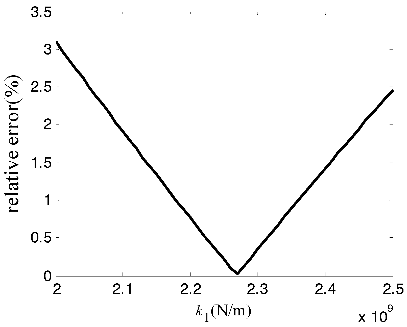
9	1	1	0.00225	813.2	7232.3

. It should be noted that the response values of $\theta$ in each set are determined according to the method shown in Figure 7 because $\theta$ has a predominant influence on Hopf bifurcation point, whereas the response value of the real part and the coupling frequency is calculated by CEA, as mentioned in Section 2.2.

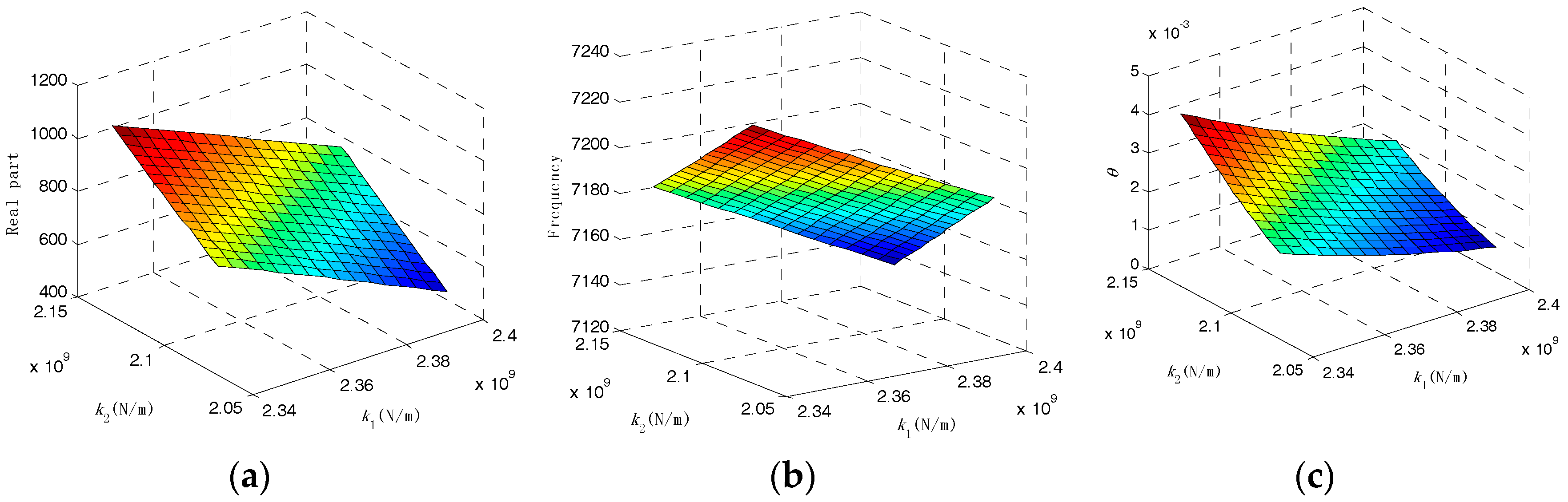
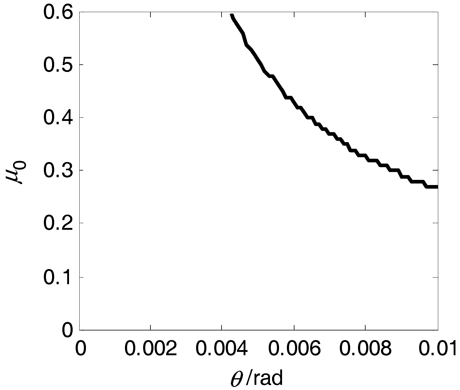
The variables and response values in Table 3 are then fitted using Equation (16). The response surface functions of the real part, frequency and slope angle $\theta$ versus stiffness $k_1$ and $k_2$ are obtained as

$$\begin{array}{ll}\mathrm{Real}\mathrm{Part}& =4.42\times {10}^4-3.66\times {10}^{-5}{k}_1-2.38\times {10}^{-7}{k}_2+4.60\times 10^{-15}{k}_1{}^2\\ & -1.03\times 10^{-15}{k}_2{}^2+4.53\times 10^{-15}{k}_1{k}_2+\epsilon \end{array}$$

(19)

$$\begin{array}{ll}\mathrm{Frequency}& =2.45\times {10}^3+1.70\times {10}^{-6}{k}_1+8.75\times {10}^{-7}{k}_2+8.54\times 10^{-17}{k}_1{}^2\\ & +3.64\times 10^{-17}{k}_2{}^2-6.46\times 10^{-16}{k}_1{k}_2+\epsilon \end{array}$$

(20)

$$\begin{array}{ll}\theta =& 0.1471-1.60\times {10}^{-10}{k}_1+4.28\times {10}^{-11}{k}_2+1.36\times 10^{-19}{k}_1{}^2\\ & 1.36\times 10^{-19}{k}_2{}^2-2.44\times 10^{-19}{k}_1{k}_2+\epsilon \end{array}$$

(21)

And the response surface plots are shown in Figure 8.

Ignore the effect of fitting error $\epsilon$, and let Equations (19) and (20) equal to the optimization objectives of finite element results, respectively. Thus, the following equations are obtained:

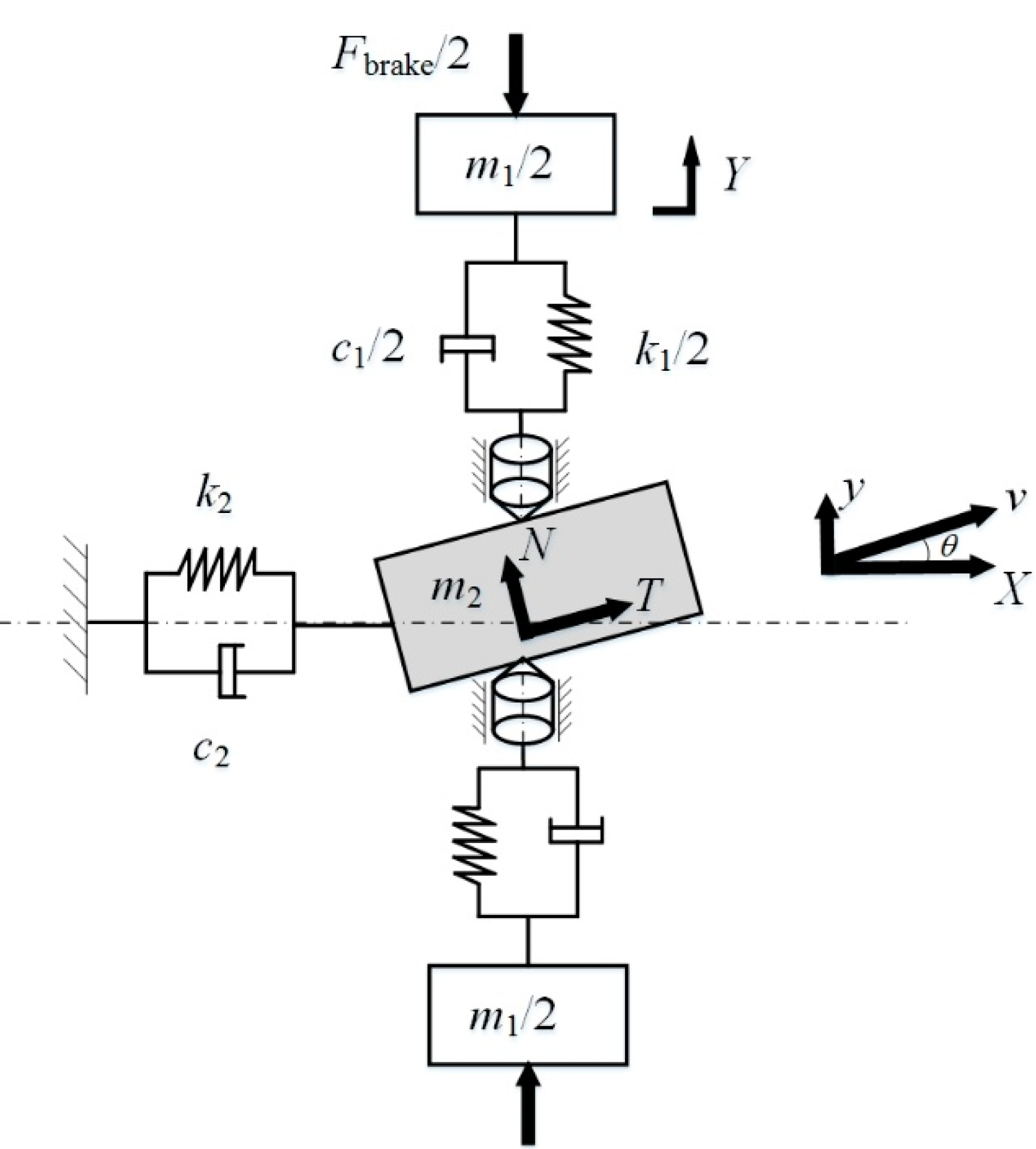
$$\{\begin{array}{l}4.42\times {10}^4-3.66\times {10}^{-5}{k}_1-2.38\times {10}^{-7}{k}_2+4.60\times 10^{-15}{k}_1{}^2\\ -1.03\times 10^{-15}{k}_2{}^2+4.53\times 10^{-15}{k}_1{k}_2=713.4\\ 2.45\times {10}^3+1.70\times {10}^{-6}{k}_1+8.75\times {10}^{-7}{k}_2+8.54\times 10^{-17}{k}_1{}^2\\ +3.64\times 10^{-17}{k}_2{}^2-6.46\times 10^{-16}{k}_1{k}_2=7168.6\end{array}$$

(22)

Values of $k_1$ and $k_2$ which meet both optimization objectives of the frequency and real part can be solved by Equation (22). The value of $\theta$ can be further obtained from Equation (21). Finally, all kinetic parameters are determined as m₁ = 1.2 kg, m₂ = 1 kg, k₁ = 2.3658 × 10⁹ N/m, k₂ = 2.0858 × 10⁹ N/m, θ = 0.0018 rad.

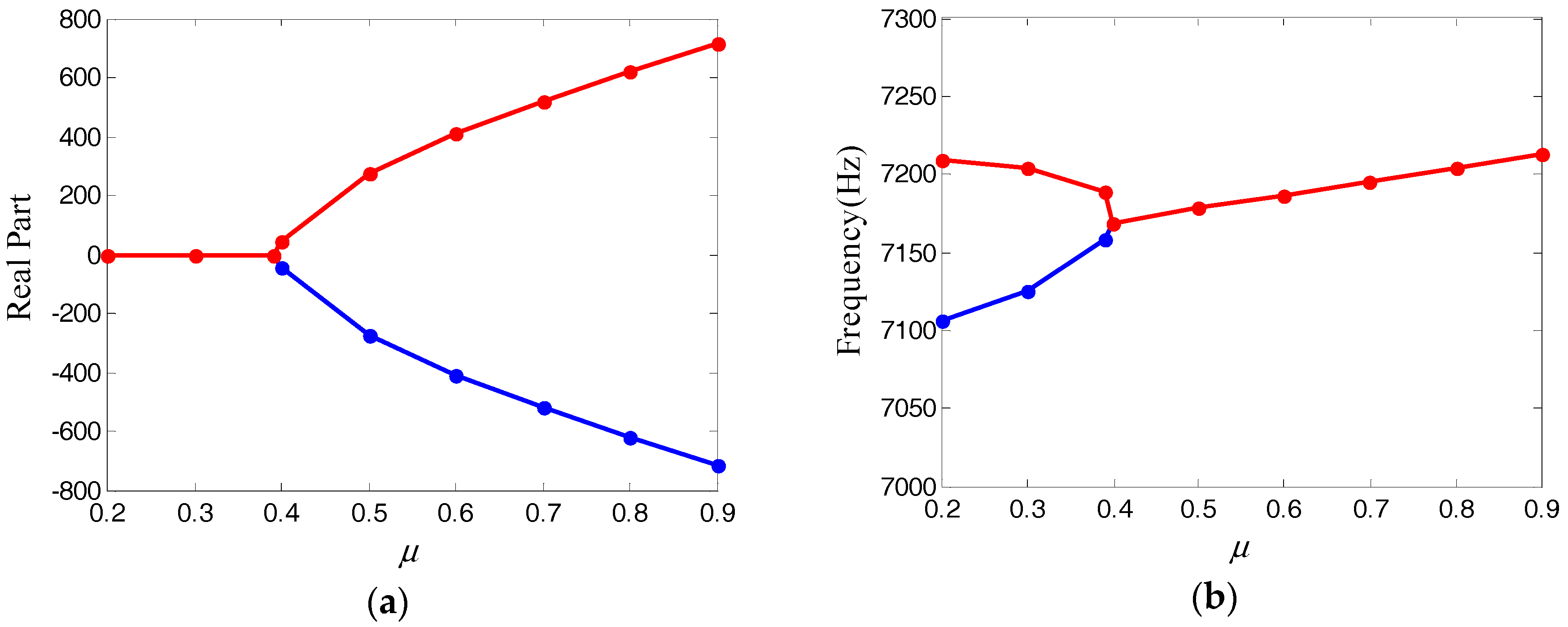
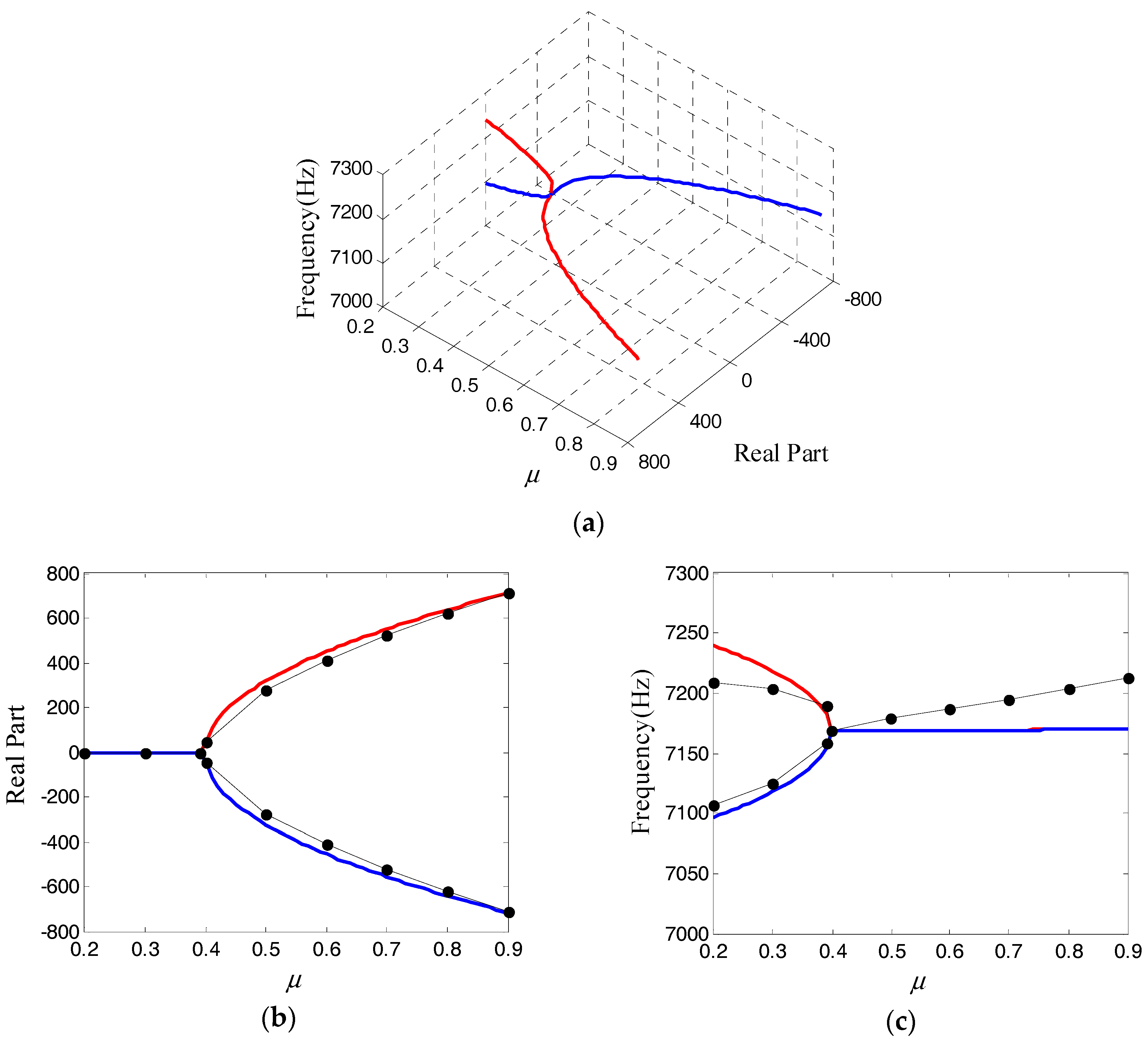
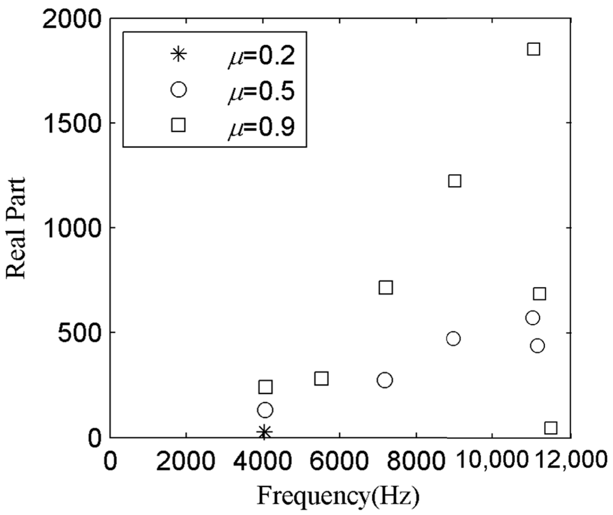
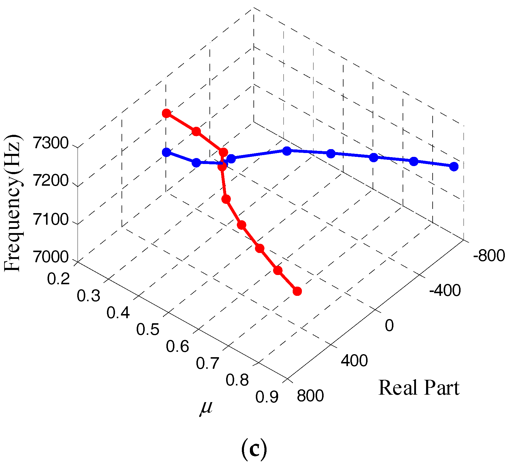
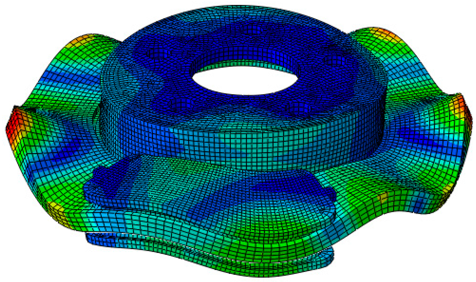
Under these optimized parameters, Figure 9a displays the evolutions of both real parts and frequencies versus friction coefficient. Moreover, a comparison between the CEA results of the minimal model and that of the finite element model is illustrated in Figure 9b,c, where the black line represents the finite element result previously given in Figure 4. It is shown that the Hopf bifurcation point of the 2-DoF model is ${\mu }_0=0.4$. In Figure 9b, when the friction coefficient is greater than 0.4, the real parts become positive and continuously increase with the increase of the friction coefficient. When the friction coefficient is 0.9, the corresponding maximum real part is 711.8. In Figure 9c, frequencies of the two close modes tend to approach each other gradually as the friction coefficient increases, and finally coupling occurs at the bifurcation point. The coupling frequency is 7168.6 Hz.

After parameter optimization, the coupling frequency, Hopf bifurcation point and the maximum real part of the minimal model are all consistent with the selected finite element mode. The error is within acceptable limits. The optimized 2-DoF model can be more easily associated with the finite element braking model with a disc and two pads. To a certain extent, it represents the coupling properties of the unstable mode with seven nodal diameters. More reliable numerical results of braking stability can be obtained by using the parameters-optimized minimal model.

4. Discussion on Stability

The existence of modal coupling phenomenon in squeal instability have been confirmed by extensive studies. Actually, when mode coupling occurs in the system, simultaneously the friction coefficient appears to have notable nonlinear variation. Experiments have also found the friction coefficient of different materials to be a function of the relative speed between the friction components [31,32]. In addition, brake squeal usually occurs at relatively low speed in a real traffic jam. This all means that the relative speed between the disc and pad plays an important role in brake squeal.

So the effect of variation of friction coefficient with braking velocity is discussed in the stability analysis of this section. TA is used to solve the dynamic response of the system. Compared with CEA, TA can obtain the amplitude of vibration velocity and displacement, which is conducive to observe the variation law of friction coefficient. However, the feasibility of TA using finite element method is reduced because the method is time-consuming. So the 2-DoF model is adopted for the following analysis. It is more efficient to investigate the effect of different braking velocities on the stability.

On the basis of the linear model mentioned in Section 3, a negative slope friction characteristic between the brake disc and pad are introduced. The equation provided by Shin [19] is

$$\mu ={\mu }_{\mathrm{s}}-{\mu }_{\mathrm{k}}\left|v-\dot{X}/\cos \theta \right|$$

(23)

where ${\mu }_{\mathrm{s}}$ is the static friction coefficient, ${\mu }_{\mathrm{k}}$ is the negative slope coefficient which represents the descent rate of friction coefficient, $v$ is the rotation velocity of the disc which is a constant, $\dot{X}/\cos \theta$ is the velocity projection of $m_2$ in horizontal direction.

Subsisting Equation (23) into Equation (3) yields a more complex friction model as the static friction coefficient is introduced. Here a simplification is made for the friction law that the stick phase (e.g., the friction force is $T<{\mu }_{\mathrm{s}}N$) is not considered, so that nonlinearity of discontinuity does not involve in the friction model, and the system can be easily integrated by a standard ODE-solver available in MATLAB [33]. Then the time-history response of the equation is solved via the classic fourth-order Runge-Kutta algorithm. The initial conditions are set as $X_0=Y_0={\dot{X}}_0={\dot{Y}}_0=0$, and ${\mu }_{\mathrm{s}}=0.4625$, ${\mu }_{\mathrm{k}}=0.025$, so that when the velocity of brake disc equals to 2.5 m/s, the initial dynamic friction coefficient is $\mu =0.4$, just at the bifurcation area. The effect of brake pressure on the stability is not the interest of this paper, and $F_{\mathrm{brake}}=100\hspace{1em}\mathrm{N}$ in this case. 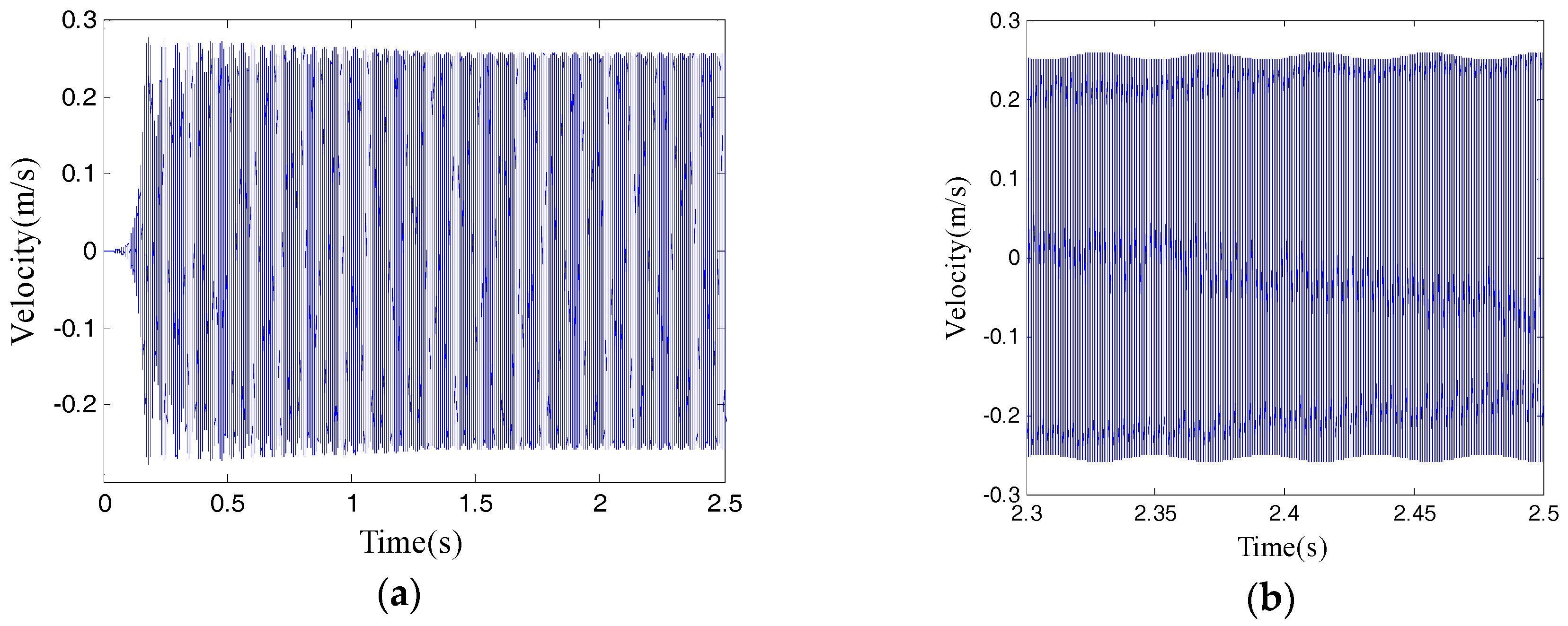Figure 10a gives the velocity response over time in the $Y$ direction at $v=2.5 \mathrm{m}/\mathrm{s}$, and Figure 10b is the response with timescale zoomed in. Since the dynamic response in the $X$ direction is similar, it is not shown. In Figure 10b, the steady state response in the $Y$ direction is a periodic signal with changing amplitude. The reason for this phenomenon is known from Equation (23), that during oscillation process of the system, the relative velocity $\left|v-\dot{x}\right|$ is constantly changing. This causes the friction coefficient to change repeatedly around the bifurcation point; namely, the system is in constant conversion between stable and unstable. When the friction coefficient exceeds the bifurcation point, the system becomes unstable, so the velocity response increases. At the same time, the friction coefficient reduces below the bifurcation point as the relative velocity increases, then the vibration response decreases.

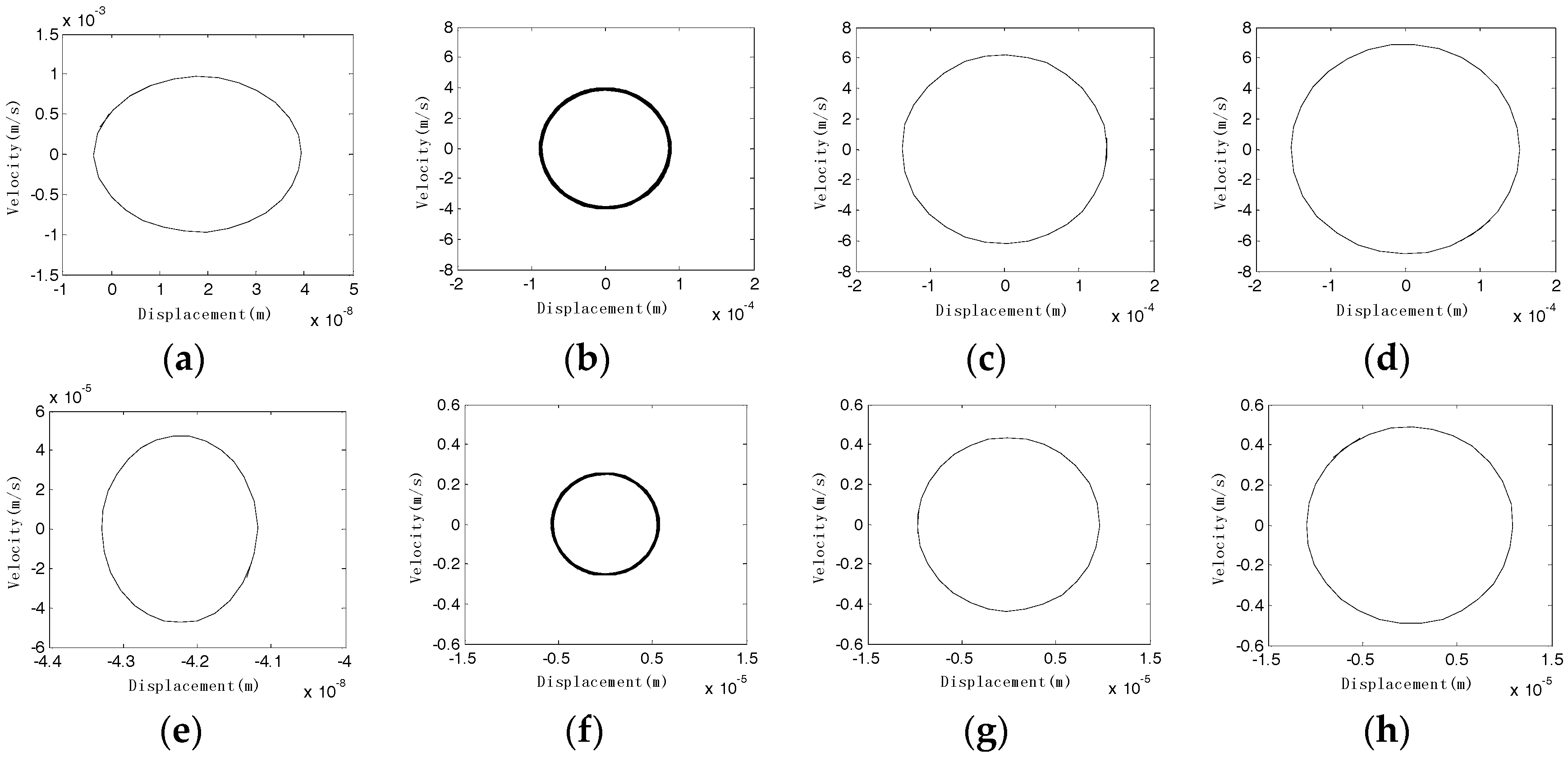
In addition, to study the effect of different velocities on oscillations, the steady-state responses for 3.5 m/s, 2.5 m/s, 1.5 m/s and 0.5 m/s are calculated, respectively. The limit cycles are shown in Figure 11a,b. It can be seen that when $v$ equals 3.5 m/s, the system is stable and the limit cycle amplitude is very small. When $v$ equals 2.5 m/s, the system is unstable, and the limit cycle amplitude is greater than that of 1.5 m/s and 0.5 m/s. With the decrease of disc velocity, the limit cycle amplitude becomes larger, that is to say, the instability increases. However, the increase of the amplitude is not proportional to the decrease of $v$. When $v$ continues to decrease to 0.5 m/s, the limit cycle amplitude no longer increases significantly. It is also found that the limit cycle of 2.5 m/s presents as a thick ring due to its amplitude changing (as seen in Figure 10), whereas the limit cycles amplitudes of 1.5 m/s and 0.5 m/s are constants. A large number of calculations show that when the rotational velocity of brake disc is greater than a critical value about 3.1 m/s, the system is stable. The brake system becomes unstable for a braking velocity lower than 3.1 m/s. Moreover, the lower the velocity is, the worse the stability appears. So the brake squeal tends to increase.

In conclusion, in the friction characteristic adopted in this paper, the friction coefficient is mainly affected by the value of ${\mu }_{\mathrm{k}}•v$. When ${\mu }_{\mathrm{k}}$ is a constant, the friction coefficient decreases with the increase of $v$. A relatively low friction coefficient can reduce the vibration amplitude of displacement and velocity of the system. If the friction coefficient is smaller than the bifurcation point, the mode-coupling phenomenon disappears. Thus, the occurrence of brake squeal is suppressed. It should be noted that the friction coefficient, as a key parameter affecting braking performance, cannot be designed too small from a safety perspective. On the contrary, a sufficient small value of $v$ can make the friction coefficient higher than the bifurcation point, and exacerbates the instability of the system. This is consistent with the fact that the brake squeal usually occurs in relatively low-speed braking conditions.

5. Conclusions

A large number of literatures use a minimal model to study the mechanism of brake squeal, but an accurate determination method of parameters in minimal models is rarely found. In the light of the CEA results of a finite element brake model, this paper established a more representative 2-DoF model. Taking the natural frequency, Hopf bifurcation point and real part of the eigenvalue of a finite element unstable mode as optimization objectives, the response surface method is applied to determine the kinetic parameters of the minimal model. So the minimal model can feature the mode-coupling phenomenon of the unstable mode with seven nodal diameters effectively. Further analysis for brake squeal based on this model is reliable.

Based on the optimized parameters, the negative slope friction characteristic is further introduced, and TA is performed for the dynamic equations of the 2-DoF model. The results show that nonlinear variation characteristics of the friction coefficient with braking speed can affect modal coupling of the system, and therefore lead to squeal instability. The squeal is more likely to occur under relatively low velocity, which is consistent with objective facts. While the relative velocity is higher than a critical value, the system is stable. Therefore, the uncertainty of braking speed is closely related to the unpredictability of the squeal.

The minimal model presented in this paper is intuitive. The model parameter determination method based on the response surface optimization fill in a gap in the literature. Moreover, compared with the FEA which consumes considerable computation time and data resources, the 2-DoF model enjoys the superiority of high efficiency in solving the dynamic response, making it easier to analyze the effect of the nonlinear variation of parameters such as friction coefficient on the limit cycle of the system. Therefore, the parameter determination method and parameter analysis results of the minimal model proposed in this paper can provide a reference for an improved design of the brake system.

References

1. Popp, K.; Stelter, P. Stick-slip vibrations and chaos. Philos. Trans. Phys. Sci. Eng. 1990, 332, 89–105. [Google Scholar] [CrossRef]
2. Ouyang, H.; Mottershead, J.E.; Cartmell, M.P.; Brookfield, D.J. Friction-induced vibration of an elastic slider on a vibrating disc. Int. J. Mech. Sci. 1999, 41, 325–336. [Google Scholar] [CrossRef]
3. Paliwal, M.; Mahajan, A.; Don, J.; Chu, T.; Filip, P. Noise and vibration analysis of a disc-brake system using a stick-slip friction model involving coupling stiffness. J. Sound Vib. 2005, 282, 1273–1284. [Google Scholar] [CrossRef]
4. Ibrahim, R.A. Friction-induced vibration, chatter, squeal, and chaos—Part II: Dynamics and modeling. Appl. Mech. Rev. 1994, 47, 227–253. [Google Scholar] [CrossRef]
5. Ouyang, H.; Mottershead, J.E.; Cartmell, M.P.; Friswell, M.I. Friction-induced parametric resonances in discs: Effect of a negative friction–velocity relationship. J. Sound Vib. 1998, 209, 251–264. [Google Scholar] [CrossRef]
6. Sinou, J.J.; Coudeyras, N.; Nacivet, S. Study of the nonlinear stationary dynamic of single and multi-instabilities for disk brake squeal. Int. J. Veh. Des. 2009, 51, 207–222. [Google Scholar] [CrossRef]
7. Spurr, R.T. A theory of brake squeal. Proc. Inst. Mech. Eng. Automob. Eng. 1961, 15, 33–52. [Google Scholar] [CrossRef]
8. Millner, N. An Analysis of Disc Brake Squeal; SAE Technical Paper No. 780332; SAE International: Warrendale, PA, USA, 1978. [Google Scholar]
9. Coudeyras, N.; Sinou, J.J.; Nacivet, S. A new treatment for predicting the self-excited vibrations of nonlinear systems with frictional interfaces: The constrained harmonic balance method, with application to disc brake squeal. J. Sound Vib. 2012, 319, 1175–1199. [Google Scholar] [CrossRef]
10. Liles, G.D. Analysis of Disc Brake Squeal Using Finite Element Methods; SAE Technical Paper No. 891150; SAE International: Warrendale, PA, USA, 1989. [Google Scholar]
11. Hoffmann, N.; Fischer, M.; Allgaier, R.; Gaul, L. A minimal model for studying properties of the mode-coupling type instability in friction induced oscillations. Mech. Res. Commun. 2002, 29, 197–205. [Google Scholar] [CrossRef]
12. Fritz, G.; Sinou, J.J.; Duffal, J.M.; Jézéquel, L. Investigation of the relationship between damping and mode-coupling patterns in case of brake squeal. J. Sound Vib. 2007, 307, 591–609. [Google Scholar] [CrossRef]
13. Hoffmann, N.; Gaul, L. Effects of damping on mode-coupling instability in friction induced oscillations. J. Appl. Math. Mech. 2003, 83, 524–534. [Google Scholar] [CrossRef]
14. Dihua, G.; Dongying, J. A Study on Disc Brake Squeal Using Finite Element Methods; SAE Technical Paper No. 980597; SAE International: Warrendale, PA, USA, 1998. [Google Scholar]
15. AbuBakar, A.R.; Ouyang, H. Complex eigenvalue analysis and dynamic transient analysis in predicting disc brake squeal. Int. J. Veh. Noise Vib. 2006, 2, 143–155. [Google Scholar] [CrossRef]
16. Liu, P.; Zheng, H.; Cai, C.; Wang, Y.Y.; Lu, C.; Ang, K.H.; Liu, G.R. Analysis of disc brake squeal using the complex eigenvalue method. Appl. Acoust. 2007, 68, 603–615. [Google Scholar] [CrossRef]
17. Ouyang, H.; Nack, W.; Yuan, Y.; Chen, F. Numerical analysis of automotive disc brake squeal: A review. Int. J. Veh. Noise Vib. 2005, 1, 207–230. [Google Scholar] [CrossRef]
18. Kinkaid, N.M.; O’Reilly, O.M.; Papadopoulos, P. Automotive disc brake squeal. J. Sound Vib. 2003, 267, 105–166. [Google Scholar] [CrossRef]
19. Shin, K.; Brennan, M.J.; Oh, J.E.; Harris, C.J. Analysis of disc brake noise using a two-degree-of-freedom model. J. Sound Vib. 2002, 254, 837–848. [Google Scholar] [CrossRef]
20. Popp, K.; Rudolph, M.; Kröger, M.; Lindner, M. Mechanisms to generate and to avoid friction induced vibrations. VDI Ber. 2002, 1736, 1–16. [Google Scholar]
21. Wagner, U.V.; Hochlenert, D.; Hagedorn, P. Minimal models for disk brake squeal. J. Sound Vib. 2007, 302, 527–539. [Google Scholar] [CrossRef]
22. Cantoni, C.; Cesarini, R.; Mastinu, G. Brake comfort: A review. Veh. Syst. Dyn. 2009, 47, 901–947. [Google Scholar] [CrossRef]
23. Oberst, S.; Lai, J.C.S. Nonlinear transient and chaotic interactions in disc brake squeal. J. Sound Vib. 2015, 342, 272–289. [Google Scholar] [CrossRef]
24. Oberst, S.; Lai, J.C.S. Chaos in brake squeal noise. J. Sound Vib. 2011, 330, 955–975. [Google Scholar] [CrossRef]
25. Sinou, J.J.; Thouverez, F.; Jézéquel, L. Methods to reduce non-linear mechanical systems for instability computation. Arch. Comput. Method Eng. 2004, 11, 257–344. [Google Scholar] [CrossRef]
26. Lei, L. Research on Disk Brake Noise. Master’s Thesis, Chongqing University, Chongqing, China, 2016. [Google Scholar]
27. Papangelo, A.; Hoffmann, N.; Ciavarella, M. Load-separation curves for the contact of self-affine rough surfaces. Sci. Rep. 2017, 7, 6900. [Google Scholar] [CrossRef] [PubMed]
28. Hongming, L.; Lijun, Z.; Zhuoping, Y. Effects of Surface Roughness on the Friction-induced Squeal Noise. Tribology 2011, 31, 473–479. [Google Scholar] [CrossRef]
29. Papangelo, A.; Ciavarella, M.; Hoffmann, N. Subcritical bifurcation in a self-excited single-degree-of-freedom system with velocity weakening-strengthening friction law: Analytical results and comparison with experiments. Nonlinear Dyn. 2017, 90, 2037–2046. [Google Scholar] [CrossRef]
30. Papangelo, A.; Grolet, A.; Salles, L.; Hoffmann, N.; Ciavarella, M. Snaking bifurcations in a self-excited oscillator chain with cyclic symmetry. Commun. Nonlinear Sci. Numer. Simul. 2017, 44, 108–119. [Google Scholar] [CrossRef]
31. Bar-Sinai, Y.; Spatschek, R.; Brener, E.A.; Bouchbinder, E. On the velocity-strengthening behavior of dry friction. J. Geophys. Res. Solid Earth 2014, 119, 1738–1748. [Google Scholar] [CrossRef]
32. Jacobson, B. The Stribeck memorial lecture. Tribol. Int. 2003, 36, 781–789. [Google Scholar] [CrossRef]
33. Leine, R.I.; Campen, D.H.V.; Kraker, A.D.; Steen, L.V.D. Stick-slip vibrations induced by alternate friction models. Nonlinear Dyn. 1998, 16, 41–54. [Google Scholar] [CrossRef]
Figure 1. Finite element model of brake.
Applsci 08 00037 g001
Figure 2. Unstable modes of the brake.
Applsci 08 00037 g002
Figure 3. Modal shape of 7168.6 Hz.
Applsci 08 00037 g003
Figure 4. Complex eigenvalue analysis (CEA) results of the unstable mode: (a) the real part of eigenvalues; (b) the frequency of eigenvalues; (c) 3D plot of the coalescence patterns of the finite element mode at 7168.6 Hz.
Applsci 08 00037 g004aApplsci 08 00037 g004b
Figure 5. Two degrees of freedom (2-DoF) model for brake squeal.
Applsci 08 00037 g005
Figure 6. Evolution of frequency error versus stiffness k 1 .
Applsci 08 00037 g006
Figure 7. Evolution of Hopf bifurcation point versus angle θ .
Applsci 08 00037 g007
Figure 8. Response surfaces of (a) Real Part; (b) Frequency; (c) θ .
Applsci 08 00037 g008
Figure 9. Evolution of real parts and frequencies versus μ : (a) 3D plot of the coalescence patterns of the minimal model at 7168.6 Hz; (b) Comparison of the real part; (c) Comparison of the frequency.
Applsci 08 00037 g009
Figure 10. (a) Time-history response in Y direction; (b) Zoom.
Applsci 08 00037 g010
Figure 11. Limit cycles of different velocity: (a) X -direction limit cycles of 3.5 m/s; (b) X -direction limit cycles of 2.5 m/s; (c) X -direction limit cycles of 1.5 m/s; (d) X -direction limit cycles of 0.5 m/s; (e) Y -direction limit cycles of 3.5 m/s; (f) Y -direction limit cycles of 2.5 m/s; (g) Y -direction limit cycles of 1.5 m/s; (h) Y -direction limit cycles of 0.5 m/s.
Applsci 08 00037 g011