1. Introduction
In structural mechanics as well as in practically all fields of engineering, the periodicity characterizes the structuring of many systems such as layered composites, crystal lattices, bladed disks, turbines, multi-cylinder engines, ship hulls, aircraft fuselages, micro and nanoelectromechanical systems, etc. Periodicity implies an infinite or finite geometrical repetition of a unit cell in one, two or three dimensions and requires appropriate approaches to investigate it. Under the hypothesis of perfect periodicity, many works provided interesting insights in the behavior of these structures. In the context of wave propagation in periodic structures, the basic works performed in linear case by Brillouin [
1] and Mead [
2] are based on the Floquet’s principle or the transfer matrix in order to compute propagation constants. Based on the transfer matrix theory, a combination of wave and finite element approaches was proposed by Duhamed et al. [
3] and used later by Goldstein et al. [
4] to calculate forced responses of waveguide structures. Casadei et al. [
5] developed analytical and numerical models based on the transfer matrix approach to investigate the dispersion properties and bandgaps of a beam with a periodic array of airfoil-shaped resonating units bonded along its length. Using the Floquet-Bloch’ theorem, Gosse et al. [
6] completely described the behavior of a heat exchanger periodic structure only from the vibroacoustic knowledge of the basic unit. Collet et al. [
7] extended the analysis to two-dimensional periodic structures with complex damping configurations and underlined the reduced computational costs allowed by the Floquet-Bloch’ theorem when representing whole structures by unit cell modeling. Recently, Droz et al. [
8] combined the Wave Finite Element Method (WFEM) with Component Mode Synthesis (CMS) to evaluate the dispersion characteristics of two-dimensional periodic waveguides.
On the other hand, the wave propagation becomes considerably complicated when the governing wave equation contains nonlinear terms (i.e., contact, material or geometric nonlinearity). In this case, complex phenomena such as localization, solitons and breathers arise and traditional Floquet-Bloch and transfer matrix wave analyses are no longer applicable. In literature, other methodologies are developed to deal with nonlinear periodic structures such as perturbation approaches. For instance, Chakraborty and Mallik [
9] investigated the harmonic wave propagation in one-dimensional periodic chain consisting of identical masses and weakly non-linear springs through single-frequency harmonic balance. They used a perturbation approach to calculate the propagation and attenuation constants. A straightforward perturbation analysis is applied by Boechler et al. [
10] to investigate amplitude-dependent dispersion of a discrete one-dimensional nonlinear periodic chain with Hertzian contact. Otherwise, as an alternative to perturbation approach for strongly nonlinear systems, Georgiades et al. [
11] proposed a combination of shooting and pseudo-arc-length continuation to examine nonlinear normal modes and their bifurcations in cyclic periodic structures. Moreover, Lifshitz et al. used a secular perturbation theory to calculate the response of a coupled array of nonlinear oscillators under parametric excitation in [
12] and of N nonlinearly coupled micro-beams in [
13] using discrete models. The method of multiple scales is used by Nayfeh [
14] to construct a first-order uniform expansion in the presence of internal resonance for the governing equations of parametrically excited multi-degree-of-freedom systems with quadratic nonlinearities. Using the same methodology, Bitar et al. [
15] investigated the collective dynamics of a periodic structure of coupled nonlinear Duffing-Van Der Pol oscillators under simultaneous parametric and external excitations. An analytico computational model was used to compute the frequency responses and the basins of attraction of two and three coupled oscillators. The authors demonstrated the importance of the multimode solutions and the robustness of their attractors. The multiple scales method was also used by Gutschmidt and Gottlied [
16] in a continuum-based model to investigate the dynamic behavior of an array of N nonlinearly coupled micro-beams. Furthermore, Manktelow et al. [
17] used the multiple scales method to investigate wave interactions in monoatomic mass-spring chain with a cubic nonlinearity. In [
18], the method was combined with a finite-element discretization of a single unit cell, to study the wave propagation in continuous periodic structures subject to weak nonlinearities. The authors proposed later robust tools for wave interactions analysis in diatomic chain with two degrees of freedom per unit cell [
19]. Recently, Andreassen et al. [
20] studied the wave interactions in a periodically perforated plate through the two-dimensional dispersion characteristics, group velocities and internal resonances investigation. Romeo and Rega [
21] identified the regions of existence of discrete breathers and guided their analysis using the nonlinear propagation region of chain of oscillators with cubic nonlinearity exhibiting periodic solutions. Furthermore, using the idea of harmonic balance in the periodic structures inspired from [
9] the Harmonic Balance Method (HBM) was combined with multiple scales method in [
22] in order to study the attenuation caused by weak damping of harmonic waves through a discrete periodic structure. The HBM was later used by Narisetti et al. [
23] to analyze the influence of nonlinearity and wave amplitude on the dispersion properties of plane waves in strongly nonlinear periodic uniform granular media. Particularly, periodic coupled pendulum structure has been the purpose of several researches in literature. Marlin [
24], for instance, proved several theorems on the existence of oscillatory, rotary, and mixed periodic motions of
N coupled simple pendulums. Khomeriki and Leon [
25] demonstrated numerically and experimentally the existence of three tristable stationary states. Jallouli et al. [
26] investigated the nonlinear dynamics of a two-dimensional array of coupled pendulums under parametric excitation and, recently [
27], the energy localization phenomenon in an array of coupled pendulums under simultaneous external and parametric excitations by means of a nonlinear Schrodinger equation. The authors show that adding an external excitation increases the existence region of solitons. Bitar et al. [
28,
29] investigated the collective nonlinear dynamics of perfectly periodic coupled pendulum structure under primary resonance using multiple scales and standing-wave decomposition. The authors studied the effects of modal interactions on the nonlinear dynamics. They highlighted the large number of multimode solutions and the bifurcation topology transfer between the modal intensities, in frequency domain. The analysis of the Basins of attraction illustrated the distribution of the multimodal solutions which increases by increasing the number of coupled pendulums. A detailed review was presented by Nayfeh et al. [
30] dealing with the influence of modal interactions on the nonlinear dynamics of harmonically excited coupled systems. Besides, the study of collective nonlinear dynamics of coupled oscillators may serve to identify the Intrinsic Localized Modes (ILMs). ILMs are defined as localizations due to strong intrinsic nonlinearity within an array of perfectly periodic oscillators. Such localization phenomenon was studied by Dick et al. [
31] in the context of microcantilever and microresonator arrays. Authors used the multiple scales method and other methods to construct nonlinear normal modes and suggested to realize an ILM as a forced nonlinear vibration mode.
It is important to note that the dynamic analysis of periodic structures is greatly simplified by assuming perfect periodicity. However, far from this mathematical idealization, imperfections, which can be due to material defects, manufacturing defaults, structural damage, ageing, fatigue, etc., and which reflect the reality of systems, can perturb the perfect arrangement of cells in a structure and change significantly the dynamic behavior from the predictions done under perfect periodicity hypothesis. In literature, primary works dealing with the issue of presence of imperfections in periodic structures treat it under the framework of disorder. Kissel [
32], for instance, investigated the effects of disorder in one-dimensional periodic structure using Monte Carlo (MC) simulations. He used a transfer matrix modeling and the limit theorem of Furstenberg to compute products of random matrices for structures carrying a single pair of waves and the theorem of Oseledets for those carrying multiplicity of wave types. The results show that disorder causes wave attenuation and pronounced spatial localization of normal modes at frequencies near the bandgaps of the perfectly periodic associated structure. Statistical investigation of the effect of disorder on the dynamics of one-dimensional weakly/strongly coupled periodic structures, using the MC method, was carried out by Pierre et al. [
33]. The effect of disorder is evaluated through the statistics of the localization factor reflecting the exponential decay of the vibration amplitude. An extension of the analysis from single degree of freedom bays to multimode bays which are more representative of periodic engineering structures was then presented in [
34]. Impact of disorder on the vibration localization in randomly mistuned bladed disks was also discussed by Castanier et al. in the review paper [
35]. Statistical investigations were made using both classical and accelerated MC methods. With the aim of computational cost saving of numerical analysis, CMS-based ROMs could then be used to calculate the mistuned forced response for each MC simulation, at relatively low cost. Moreover, to study the effects of the randomness of flexible joints on the free vibrations of simply-supported periodic large space trusses, Koch [
36] combined an extended Timoshenko beam continuum model, MC simulations and first-order perturbation method. These works proved that the normal modes, which would be periodic along the length of a perfectly periodic structure, are localized in a small region when periodicity is perturbed. Moreover, Zhu et al. [
37] studied the wave propagation and localization in periodic and randomly disordered periodic piezoelectric axial-bending coupled beams using a finite element model and the transfer matrix approach. The localization factor characterizing the average exponential rate of decay of the wave amplitude in the disordered periodic structure was computed using the Lyapunov exponent method. The authors proved that the wave propagation and localization can be altered by properly adjusting the structural parameters.
In the context of disorder in periodic coupled pendulums structures, Tjavaras and Triantafyllou [
38] investigated numerically the effect of nonlinearities on the forced response of two disordered pendulums coupled through a weak linear spring. Disorder generates modal localization and reveals large sensitivity to small parametric variations. In [
39], the authors demonstrated that an impurity introduced by longer pendulum in the chain of coupled parametrically driven damped pendulums supporting soliton-like clusters expands its stability region. Whereas impurity introduced by shorter pendulum defects simply repel solitons producing effective partition of the chain. Hai-Quing and Yi [
40] developed a discrete theoretical model based on the envelope function approach to study analytically and numerically the effect of mass impurity on nonlinear localized modes in a chain of parametrically driven and damped nonlinear coupled pendulums. The influence of impurities on the envelope waves in a driven nonlinear pendulums chain has been investigated numerically under a continuum-limit approximation in [
41] and then experimentally in [
42].
Design of engineering structures with periodicity, nonlinearity and uncertainty is a complex challenge and the main aim of this work is to deal with. Under the hypothesis of small imperfections, the collective dynamics and the localization phenomenon due to the weak coupling of components is preserved. To investigate the collective dynamics of perfectly periodic nonlinear
N degrees of freedom systems and control modal interactions between coupled components, previous works [
12,
15,
28,
29] proposed discrete analytical models combining the multiple scales method and standing-wave decomposition. The main objective of the present work is to extend these methodologies to the presence of imperfections by proposing a more generic discrete model. If, in particular, imperfections are taken into account in a probabilistic framework as parametric uncertainties modeled by random variables, uncertainty propagation methods must be applied. Uncertainties are thus propagated through the proposed generic model to evaluate the robustness of the collective dynamics against the randomness of the uncertain input parameters. The established generic discrete analytical model leads to a set of coupled complex algebraic equations. These equations are written according to the number and positions of the imperfections in the structure and then numerically solved using the Runge-Kutta time integration method. To propagate uncertainties through the established model, the statistical Latin Hypercube Sampling (LHS) method [
43] is used as a reference with respect to which the efficiency of the generalized Polynomial Chaos Expansion (gPCE) [
44,
45] is evaluated.
Uncertainty effects on the nonlinear dynamics of two and three coupled pendulums chains are investigated in this paper. Dispersion analyses of the frequency responses, in modal and physical coordinates, and the basins of attraction are carried out. Moreover, in order to highlight the complexity of the multimode solutions in terms of attractors and bifurcation topologies, a thorough analysis through the basins of attractions is performed. The robustness of the multimode branches against uncertainties around a chosen frequency in the multistability domain is investigated.
2. Mechanical Model
Figure 1 illustrates a generic structure for
coupled pendulums of identical length
, mass
. and viscous damping coefficient
generated by the dissipative force acting on the supporting point of each one. The pendulums are coupled by linear springs of stiffness
and are subject to an external excitation
each one. The inclination angle
. from the equilibrium position quantifies the rotational displacement of the
pendulum. Applied boundary conditions are such as the pendulum labeled
. and
are fixed so that
. The periodicity of the structure is broken by presence of
pendulums containing parametric uncertainties which can, for instance, be the pendulum’s length
as illustrated in
Figure 1.
In perfect periodicity case, one can refer to works performed in [
12,
15,
28,
29] to investigate the collective dynamics of the periodic nonlinear coupled-pendulums chain. Nevertheless, such analyzes are no longer suitable if periodicity is disturbed. The main objective of the present work is to propose a generic model which is adapted to the presence of uncertainties.
Uncertainties are supposed to affect structural input parameters, here some pendulums’ lengths, and to vary randomly. A probabilistic modeling of uncertainties, by random variables, is used and implies applying stochastic uncertainty propagation methods to evaluate the effect of the randomness in structural input parameters on the collective dynamics of the nonlinear coupled-pendulums chain.
Developing the generic model, through which uncertainties will be propagated, is based on the fact that the pendulums behave in different ways, depending on the position of each one with respect to uncertainties localization. Indeed, the equations of motion of the system are written according to the number and positions of uncertainties in the structure.
2.1. Equations of Motion
Applying the Lagrange approach leads to the equation of motion of the
nth pendulum:
where
,
,
,
if the
nth pendulum is deterministic and
,
,
,
if the length of the
nth pendulum, of stochastic displacement
, is uncertain.
Since linear coupling between pendulums is very weak and small imperfections are considered, each angular frequency is supposed to be equal to the eigenfrequency ().
The linear coupling term depends on the positions of the stochastic pendulums in the chain. If stochastic pendulums are not adjacent, four different configurations are distinguished:
- a.
If the concerned pendulum is deterministic as well as its neighbors, ;
- b.
If the concerned pendulum is deterministic but the previous one is stochastic, ;
- c.
If the concerned pendulum is deterministic but the following is stochastic, ;
- d.
If the stochastic pendulum is concerned, the deterministic displacement
is replaced by the stochastic one,
, in Equation (1) such as
and
, in this case.
The displacement
can be expressed as a sum of standing wave modes with slowly varying amplitudes [
12,
15,
28,
29]. Taking into account the boundary conditions
, the standing wave modes are:
The displacement
of the
pendulum is thus expressed as
if it is deterministic, and as
if it is affected by uncertainties.
2.2. Multiple Scales Method Applied to Stochastic Model
The multiple scales method [
46,
47] consists on replacing the single time variable by an infinite sequence of independent time scales (
), where
is a dimensionless parameter assumed to be small, and eliminating secular terms in the fast time variable
.
Limiting the study to a first order perturbation, (
), Equation (1) takes the form
where the excitation frequency
is expressed as:
,
being the detuning parameter.
The solution of Equation (6) can generally be given by a formal power series expansion:
. Up to the order
, the solution is of the form
Its derivatives are given by
with
,
,
et
.
Substituting Equations (7)–(9) into Equation (6) and separating the terms with different orders of
, one obtains a hierarchical set of equations. For the order
, an unperturbed equation is obtained
The solution of Equation (10), which appears in every order in the expansion of the approximate solution, is expressed as
for the order
, one obtains an equation of the form
Substituting Equations (4) and (5) into Equation (12) leads to
equations of the form
where the secular terms (coefficients of
) should be equated to zero to satisfy the condition of solvability of the multiple scales method. Projecting the response on the standing-wave modes implies to multiply all terms by
and sum over
. Consequently, a generic complex equation of the
amplitude
is obtained:
where
is the delta function [
12,
15] defined in terms of the Kronecker deltas as
with
is the Kronecker delta equal to
if
and to
otherwise. The functions
and
are defined in the
Appendix A.
2.3. Uncertainty Propagation
To propagate uncertainties through the established model, one can use, in a probabilistic framework, stochastic uncertainty propagation methods. Statistical methods, such as the MC method [
48] and the LHS method [
43], are the most frequently used in the literature and are considered as reference since they permit to achieve a reasonable accuracy. The LHS method consists on generating a succession of deterministic computations
according to a set of random variables
to approximate the
amplitude
. The LHS method permits to reduce the computing time required by the very time-consuming MC method by partitioning the variability space into regions of equal probability and picking up one sampling point in each region. Nevertheless, it remains computationally unaffordable since the accuracy level is proportional to the number of generated simulations. To overcome this prohibitive computational cost without a significant loss of accuracy, the gPCE is used in this work [
44,
45]. The gPCE combines multivariate polynomials and deterministic coefficients. Indeed, it approximates the
amplitude
using a decomposition, practically truncated by retaining only polynomials terms with degree up to
:
where
are the unknown deterministic coefficients and
the multivariate polynomials of
independent random variables
.
Solving the gPCE consists on computing the deterministic coefficients
. To do this, one can use intrusive or non-intrusive approaches. The former implies model modifications. However the latter considers the initial model as a black box. The regression approach is one of the most commonly used non-intrusive methods. In its standard form, it consists in minimizing the difference between the gPCE approximate solution and the exact solution. The latter is a set of deterministic solutions
corresponding to
realizations of random variables
forming an experimental design (ED). The approximate solution takes, consequently, the form
where
is called the data matrix and
is its Moore-Penrose pseudo-inverse.
In order to ensure the numerical stability of the regression approximation, the matrix must be well-conditioned. Therefore, the ED should be well selected and have the size .
The ED selection technique used in this work is based on two conditions:
- (i)
classification of all possible combinations of the roots of the Hermite polynomial of degree
so as to maximize the variable [
49,
50,
51]:
- (ii)
minimization of the number:
where
is the 1-norm of the matrix, in order to ensure that the invertible matrix
is well-conditioned [
51,
52].
A number of roots’ combinations, which verify the conditions in Equations (18) and (19), create then the ED.
Statistical quantities, such as the first and second moments (the mean and the variance, respectively), could then be calculated to quantify the randomness of the stochastic responses.
2.4. Solving Procedure
To solve Equation (14), a transformation of the complex amplitude to Cartesian form is needed:
Substituting Equation (20) into Equation (14) and simplifying by
, one can obtain two generic equations for the real and imaginary parts of each amplitude
:
consequently,
coupled algebraic equations are obtained.
Solving analytically these equations is very difficult or even impossible, especially in presence of uncertainties. To overcome this issue, numerical solving processes must be used. Subsequently, two possible configurations occur regarding including or not the stability analysis. To solve similar problem, Bitar et al. [
15,
29] applied the Asymptotic Numerical Method (ANM) [
53,
54,
55,
56] in graphical interactive software named MANLAB [
57] and included stability analysis. The complexity of the study was underlined in presence of multiplicity of stable and unstable solutions. In the present work, accounting for uncertainties increases the number of stable and unstable branches and thus makes the solving ANM-based process very difficult, prohibitive or even impossible. To simplify the study, we choose to limit the solving process to the computation of stable solutions and to apply the Runge-Kutta time integration method to solve Equations (21) and (22).
3. Numerical Examples
Two numerical examples are considered in this section: two and three coupled pendulums chains. To make clear presentation and discussion of each example, deterministic study is presented at first. Stochastic results are then discussed compared to deterministic ones to evaluate the robustness of the collective dynamics of the considered structures against uncertainties.
In deterministic case, the design parameters of the perfectly periodic structure are listed in
Table 1 [
29].
In stochastic case, the length of the first pendulum is supposed to be uncertain and varies such as
where
is a chosen dispersion level and
a lognormal random variable.
Uncertainty propagation through the generic discrete model is performed using the LHS method and the gPCE. Effects of uncertainties on the collective dynamics of the structures are investigated through statistical analyses of the dispersions of the frequency responses and the basins of attraction.
The problem is numerically time-consuming when using the Runge-Kutta time integration method. It is also necessary to sufficiently refine frequency steps and vary initial conditions to obtain more stable solutions, although it is difficult to cover all possible solutions. These constraints impose minimizing as possible the number of samples for the LHS method. Therefore, 200 samples are generated.
To apply the gPCE method, a fourth order expansion is used (). The length of the first pendulum is considered to be an uncertain parameter (). Hence, Hermite polynomial roots are chosen, according to which deterministic solutions are computed. Consequently, the 200 samples required for the LHS method are reduced by 97.5%.
3.1. Example 1: Two Coupled Pendulums
Two coupled pendulums structure (N ) is considered here. algebraic equations are generated with stochastic pendulum, deterministic pendulum neighbor of the stochastic one and since no deterministic pendulum in the structure has deterministic neighbors.
3.1.1. Deterministic Study
If uncertainty is not taken into account,
,
and
. Consequently, 4 algebraic equations are generated. Deterministic responses in both modal and physical coordinates are illustrated in
Figure 2.
A multiplicity of stable solutions is generated, in the multistability domain, by modal interactions [
58] between the responses which are driven by the collective dynamics. Three stable solutions could thus be obtained at several frequencies in the multistability domain [
59,
60,
61]. They are classified as Single (SM) and Double mode (DM) solutions. The only SM branch, presented by red curve, corresponds to the null trivial solution of the second amplitude. Two SM branches are identified for the first amplitude: resonant branch (SM-RB) and non-resonant branch (SM-NRB) (
Figure 2a). The DM branches, which are presented by blue curves, result from coupling between the pendulums. A correspondence in term of bifurcation points between the amplitudes with respect to each branch type is observed. It is generated by the bifurcation topology transfer. Identical physical responses reflect the symmetry between the pendulums.
More detailed illustration of the bifurcation topology transfer between the amplitudes
and
is allowed by the basins of attraction. The robustness of the attractors, corresponding to the multimode branches, and their contributions in the basins are investigated. In literature, Bartuccelli et al. [
62] illustrated numerically the basins of attraction of a plane pendulum under parametric excitation. An experimental investigation of the basins of attraction of two fixed points of a nonlinear mechanical nano-resonator was illustrated by Kozinsky et al. [
63]. Sliwa et al. [
64] studied the basins of attraction of two coupled Kerr oscillators. Bitar et al. [
15] studied the basins of attraction of two and three coupled oscillators under both external and parametric excitations. The basins of attraction are generally plotted in the phase plan (
). In this work, the basins of attraction are plotted in the Nyquist plane
of real and imaginary parts of the responses amplitudes
[
15,
29] regarding the proposed solving methodology.
Fixing the detuning parameter on
, in the multistability domain, two and three stable solutions are obtained for
and
, respectively. Two and three attractors correspond to these stable solutions, respectively, in the basins of attraction.
Figure 3 illustrates the basins of attraction plotted in the Nyquist plane
for
.
When jumps between SM-RB and SM-NRB, is stabilized on SM. Similarly, a correspondence exists between the DM attractors. Subsequently, one can restrict the analysis to the basins of attraction of .
Varying the detuning parameter (
,
and
), the contribution of each attractor is illustrated quantitatively through the ratio of its size with respect to the global size of the basins of attraction. For
, the most robust attractors correspond to the SM-NRB; they dominate the basins with 52.5% of their total size, compared to 45.9% and only 1.6% for the SM-RB and DM attractors, respectively. Nevertheless, the SM-NRB attractors vanish for
and the DM attractors become the most robust; their contribution is quantified by 64.5%, compared to a contribution of 35.5% of the SM-RB. For
,
Figure 3, the DM attractors also dominate the basins of attraction; 60.9%. However, the contributions of the attractors of SM-RB and DM are quantified by 15.7% and 23.4%, respectively.
3.1.2. Stochastic Study
Impact of uncertainty is illustrated by the envelopes of the frequency responses amplitudes computed using the LHS method and the gPCE, in generalized and physical coordinates, for two dispersion levels:
and
(
Figure 4,
Figure 5 and
Figure 6).
In order to enable comparative study with deterministic responses, we use the initial conditions fixed in deterministic case, in the multistability domain. The discontinuity of the envelopes is due to the lack of initial conditions. Note that varying more the initial conditions makes computation prohibitive and it still difficult to cover all possible solutions and so obtain smooth curves.
Increasing the dispersion level affects more the responses variability. All multimode branches are larger in terms of amplitude and frequency. Consequently, the multimode solutions are enhanced and the multistability domain is wider. The uncertainty effect on each pendulum response depends on its position with respect to the stochastic one. The greatest impact is on the first pendulum responses (larger envelopes) since it contains the uncertain parameter. The second one is less affected by uncertainty. Modal localization is consequently generated on the first pendulum response.
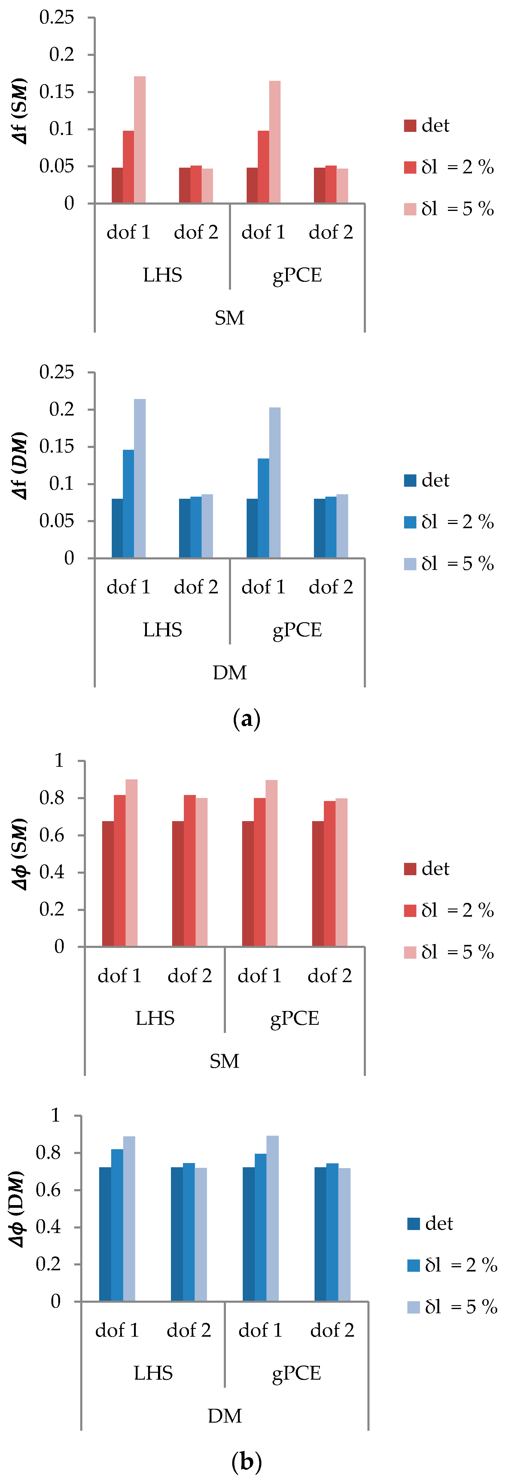
Table 2 and
Figure 7 and
Figure 8 illustrate the uncertainty effects through the intervals of variation of the amplitude (
) and frequency (
) ranges of the multistability domain. These intervals are computed between extreme bifurcation points, according to the example shown in
Figure 7.
is more affected by uncertainty than
since the first pendulum length is stochastic. More important variation is detected on
than on
. The ratio
shows that the nonlinearity of the first pendulum response is strongly strengthened. Moreover, dispersion and nonlinearity are proportional.
Satisfying approximations are allowed by the gPCE with respect to the LHS method, considered as reference. Good agreement between modal and physical responses is proved by small accuracy errors. For , the gPCE errors increase, revealing the limits of the method against high level of uncertainty. It is important to note that some errors result from the luck of initial conditions making the detection of bifurcation points more difficult.
In presence of uncertainty, a set of solutions is generated by the LHS method or the gPCE. Several basins of attraction are thus superposed. The envelopes of the attractors are quantified by the overlapped areas. For , the envelopes of the attractors of (first pendulum), computed using the LHS method, represent 64.57% of the basins. The gPCE approximation gives 62.34%. The envelopes of the attractors of (second pendulum) represent 9.67% of the basins (gPCE: 8.97%). For , the impact of uncertainty is more important. Indeed, the basins of attraction of are fully overlapped (100%). The size of the envelopes of the attractors of , computed by the LHS method, increases to 19.04%. The gPCE approximate it by 17.55%. The gPCE gives a satisfying approximation of the basins’ envelopes, although errors proportionally increase with dispersion level. The comparison of the envelopes of the basins of to those of highlights the modal localization generated on the first pendulum response.
Moreover, 96.4% of CPU time reduction is achieved when applying the gPCE, with respect to the LHS method. In fact, nearly are needed to compute the frequency responses using the LHS method. However, less than is required for the gPCE implementation. More important time reduction ratio is achieved when computing the basins of attraction: 97.6%. Indeed, the required by the LHS method are reduced to only needed for the gPCE implementation. Note that all computations are made using Matlab on 8-Core Dual Processor with 64 GB of RAM (Random Access Memory).
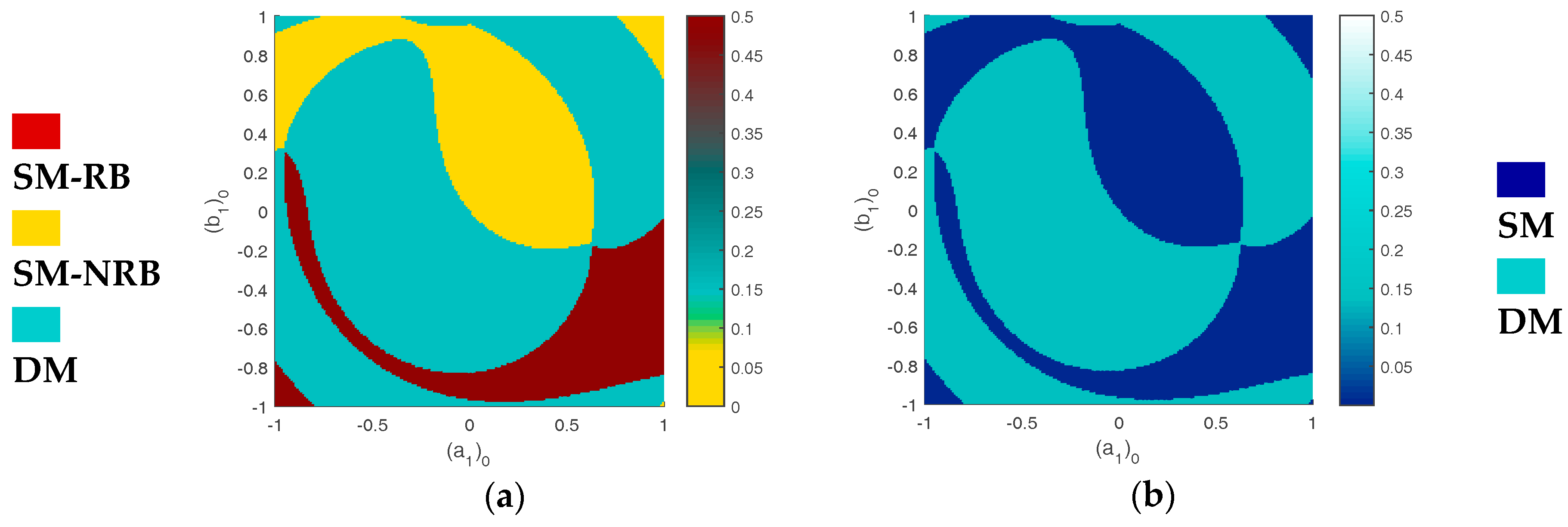
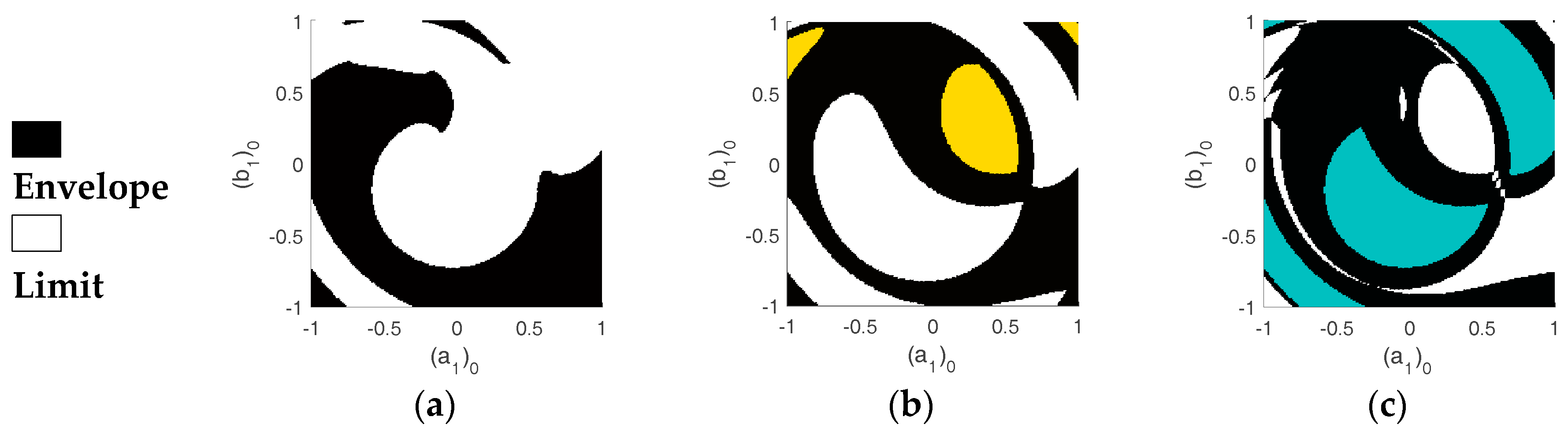
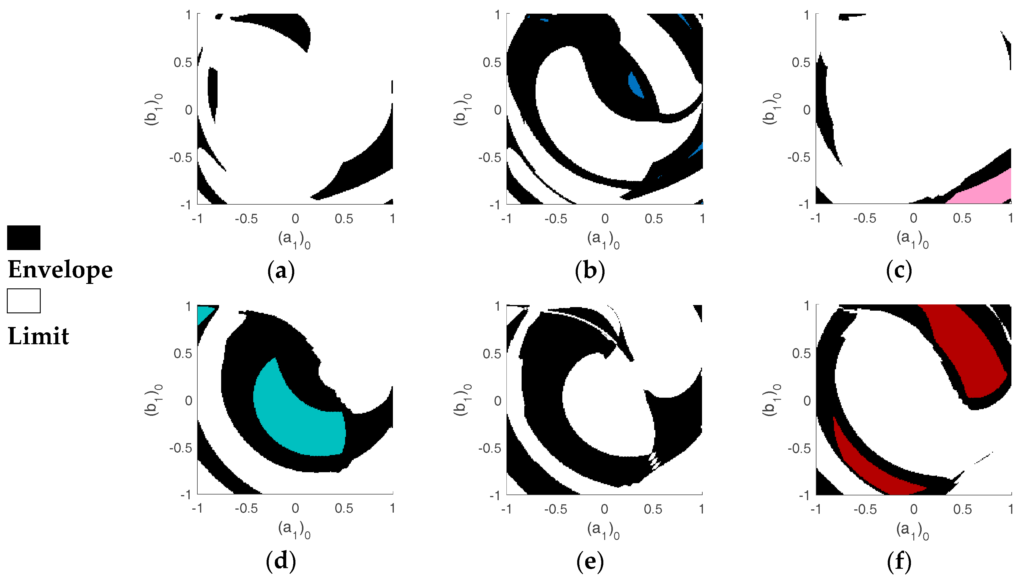
For more detailed dispersion analysis, the attractors of SM-RB, SM-NRB and DM are plotted separately. The variability of the basins of attraction of
is more important than the variability of the basins of
, which illustrates modal localization on first pendulum response. The dispersion of each attractor is illustrated by the variability of its contribution in the basins of attraction from a minimal size (color defined for the considered attractor in the deterministic case illustrated by
Figure 3) to a maximal size bounded by the limit (white area) corresponding to other attractors’ contributions. The envelopes are represented by black areas.
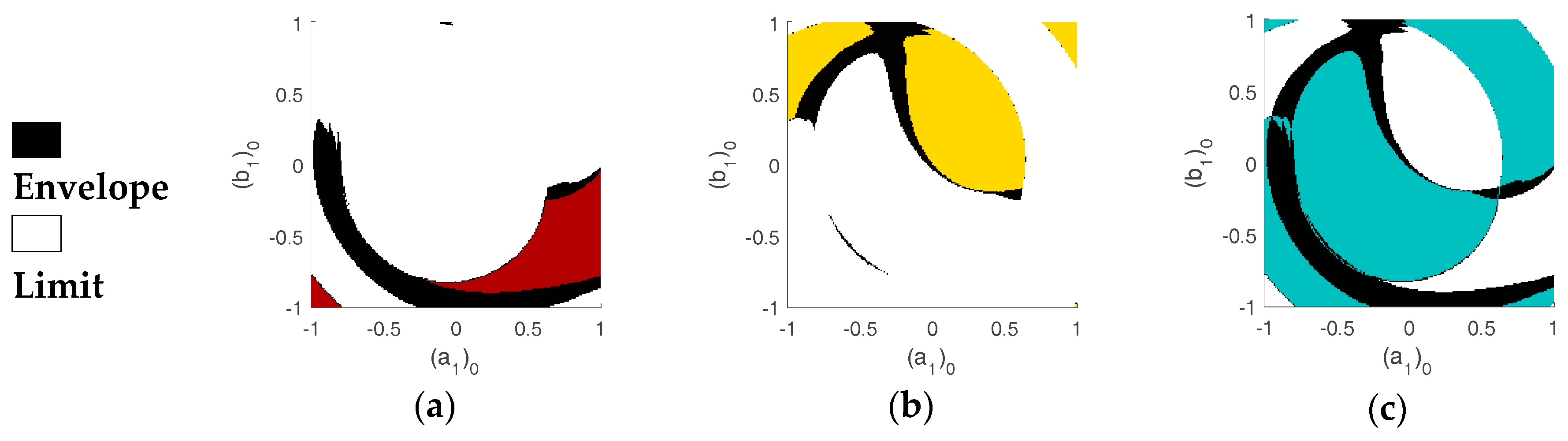
Figure 9 shows the envelopes of the attractors of
, for
, computed using the gPCE. Since, the basins of
are fully overlapped for
,
Figure 10 illustrates the envelopes of the basins of
.
As shown in
Figure 9, the DM attractors are the most robust.
Table 3 compares the contributions of the attractors of SM-RB, SM-NRB and DM in the basins of attraction in deterministic and stochastic case (for
and
).
Table 3 lists both minimal sizes and envelopes of the attractors. Summing these two areas gives the global contribution of each attractor in the basins. Superposing the envelopes of the attractors of SM-RB, SM-NRB and DM gives the global envelopes.
In deterministic case, the DM attractors of the first pendulum response are the most robust. However, the contributions of the attractors of SM-RB and SM-NRB in the basins become more important for and even more for . The SM-NRB attractors are in fact the most robust. The DM attractors of the second pendulum response remain the most robust. This evolution of the attractors’ contributions in the basins of attraction is due to modal localization generated by presence of uncertainty.
Table 3 proves that more accurate approximation of the variability of the basins of attraction is obtained using the gPCE for lower dispersion level (
, here). The gPCE approximations of the basins of attraction are more affected than those of the frequency responses. The basins analysis is indeed more thorough.
3.2. Example 2: Three Coupled Pendulums
Three coupled pendulums structure () is considered in this section. If uncertainty is not taken into account, 6 algebraic equations are generated (, and ). In stochastic case, algebraic equations are generated with stochastic pendulum, deterministic pendulum neighbor of the stochastic one and since one deterministic pendulum in the structure has deterministic neighbors.
3.2.1. Deterministic Study
Deterministic modal and physical responses are illustrated by
Figure 11. The symmetry between the first and the third pendulum generates conformity between their physical responses.
Modal interactions and bifurcation topology transfer between the pendulums’ responses, which are driven by the collective dynamics, generate up to six stable solutions at several frequencies in the multistability domain. The obtained stable branches are classified as Double (DM) and Triple mode (TM) solutions. The DM branches correspond to the solutions of the first and third amplitudes (red curves), whereas the TM solutions result from the coupling between the pendulums (blue curves). Three DM solutions (DM-RB, DM-NRB, DM-B1 and DM-B2) and two TM solutions (TM-B1 and TM-B2) are obtained,
Figure 11a. A correspondence in term of bifurcation points between the amplitudes with respect to each branch type is observed. This is generated by the bifurcation topology transfer.
Figure 12 illustrates the contributions of the attractors of the six stable branches in the basins of attraction. The basins are plotted for
, in the Nyquist plane
for arbitrary chosen initial conditions
and
.
Figure 12 shows also the responses amplitudes, which can be identified through the color bar.
The bifurcation topology transfer between the responses generates a correspondence between the attractors in the three basins of attraction. Indeed, when and jump between DM-RB, DM-NRB, DM-B1 and MD-B2, is stabilized on DM. Moreover, a correspondence exists between the TM attractors (TM-B1 and TM-B2) of the three pendulums responses.
The DM attractors are the most robust since they dominate the basins with 51% of their global size. The contribution of the TM attractors is nearly similar (49%). Focusing on DM, the DM-B2 attractors, occupying nearly 35% of the basins, are the most robust. Similarly, the TM-B2 attractor occupies 33%. The lowest contribution is of the DM-RB attractors representing less than 2% of the global basins size.
3.2.2. Stochastic Study
The greatest impact of uncertainty is obtained on the first pendulum responses since it contains the uncertain parameter. The second pendulum responses are less affected while the behavior of the third pendulum remains deterministic, because no coupling terms relate its equation with the one associated to the stochastic pendulum. Hence, the third pendulum responses are not presented hereafter.
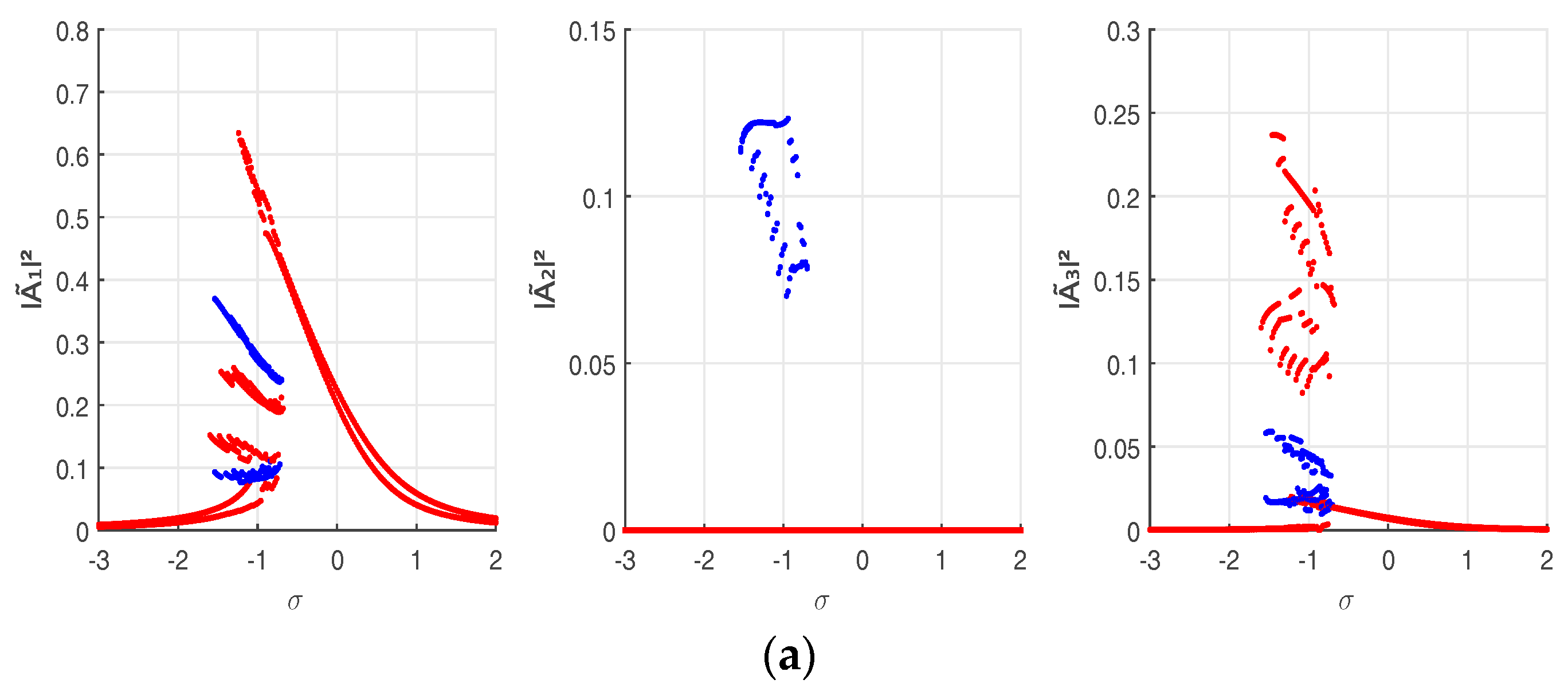
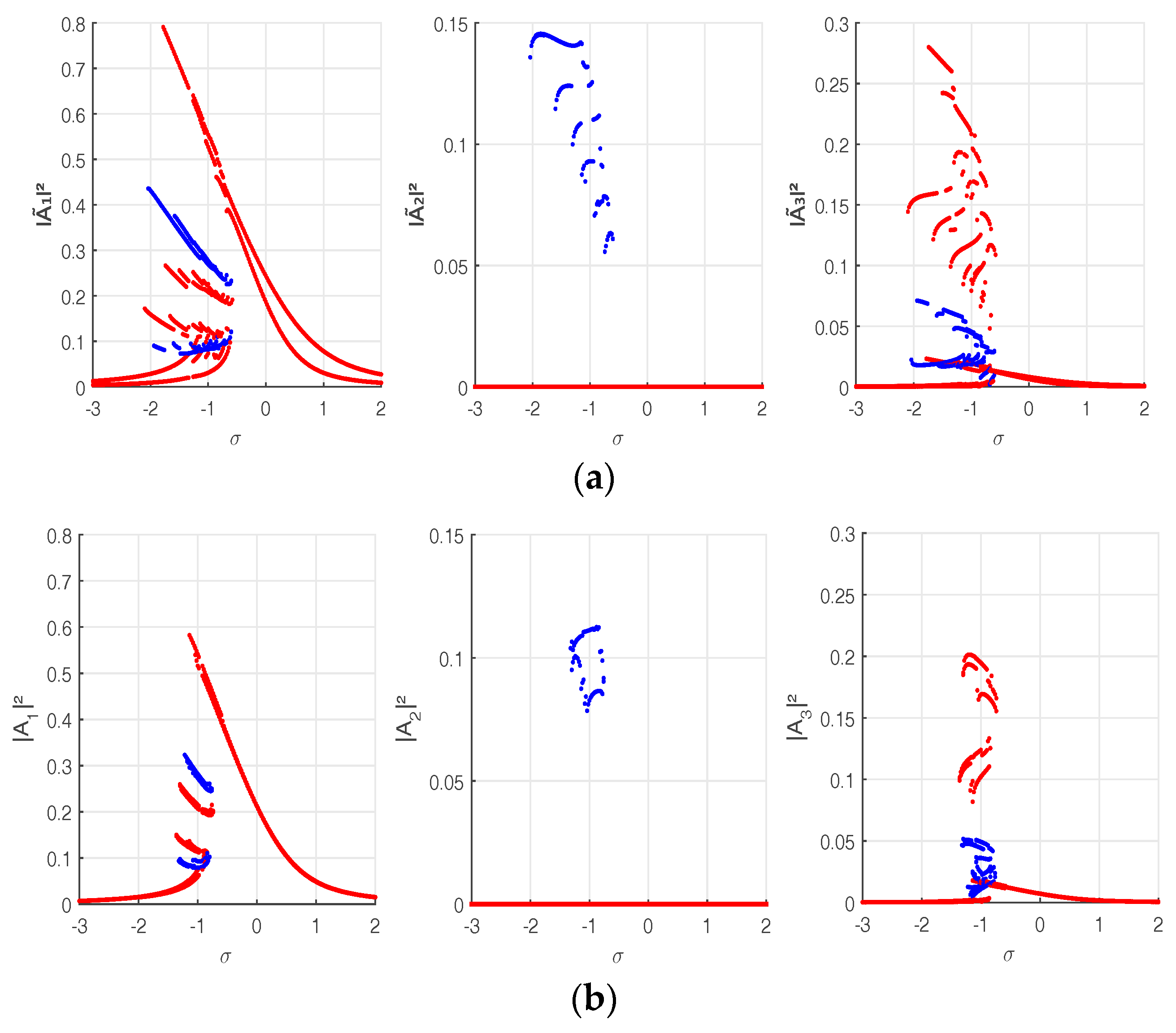
Figure 13,
Figure 14 and
Figure 15 illustrate the envelopes of the responses amplitudes in generalized and physical coordinates, for
and
.
For , all branches are larger in terms of amplitude and frequency ranges. Consequently, the multimode solutions are enhanced and the multistability domain is wider. Nevertheless, the overlap of envelopes makes detection of extreme statistics of adjacent branches more difficult. Modal localization is here generated on the response of the first pendulum containing uncertainty.
Figure 16 and
Table 4 illustrate the uncertainty effects through the intervals
and
of the multistability domain. More important variation is detected on
than on
. The ratios
show that the nonlinear aspect of the structure is enhanced. Indeed, the nonlinearity of the first pendulum response is more strengthened than the one of second pendulum response.
Comparing uncertainty propagation methods, the gPCE allows generally an accurate approximation of the responses dispersion. Nevertheless, less accuracy is obtained for . Note that errors result also from lack of initial conditions and make detection of bifurcation points difficult. Furthermore, only 5 simulations are generated when applying the gPCE, compared to 200 samples used by the LHS method. A discontinuity of the envelopes’ curves is thus detected, especially for .
Regarding the dispersion of the basins of attraction (
Figure 17 and
Table 5), the envelopes of the attractors of
, computed using the LHS method, cover 69.27% of the basins, for
. The gPCE approximation gives 66.85%. For
, the basins are fully overlapped. However, the envelopes cover only 7.58% of the basins of
, computed using the LHS method, for
and 16.40% for
. The gPCE approximations are, respectively, 6.91% and 15.02%. Less accurate results are thus obtained by the gPCE for
. To overcome this issue, one can elevate the polynomial order of the gPCE or use one of its recently developed variants [
65,
66,
67].
As shown in
Figure 17 and
Table 5, a largest dispersion is detected on the DM-RB and DM-NRB attractors of
. Their contributions in the basins, approximated in deterministic case by 1.69% and 8.71% respectively, increase up to 14.5% and 47.5%, for
. For
, the attractors become totally overlapped (100%). The DM-B2 and TM-B2 attractors of
, remain the most robust against uncertainty. The robustness analysis of the basins of attraction illustrates the modal localization generated on one or more attractors, for different dispersion levels.
On the other hand, the gPCE allows reducing the CPU time needed for the LHS method by nearly 95.2% (from down to ) and 97.5% (from down to ) when computing the frequency responses and the basins of attraction, respectively.
3.3. Overall Discussion
Three stable solutions are obtained at several frequencies in the multistability domain due to modal interactions between the responses of two coupled nonlinear pendulums, generated by the collective dynamics. However, up to six stable solutions are obtained if a three coupled pendulums chain is considered.
In presence of uncertainties, the stability of the system is enhanced. Indeed, a multiplicity of stable solutions is obtained and the multistability domain is wider in terms of frequency range and response amplitude. Moreover, the nonlinearity of the system is strengthened by increasing the ratios of the frequency intervals by the amplitude intervals computed between the extreme bifurcation points in the multistability domain.
The robustness of the attractors of different modes and modal branches is illustrated by the dispersion analysis of the basins of attraction and the quantitative study of the evolution of the distribution of these attractors from deterministic case to the case . Modal localization is generated by widening one or more special modal branches more than the others.
For a reduction of up to 97.5% of computing time compared to the LHS method, the gPCE method allows satisfying approximations of the frequency responses and the basins of attraction. These approximations are more accurate for the frequency responses since the dispersion analysis of the basins of attraction is more thorough. For high dispersion levels (>2%), some limits of the gPCE method are reached.
4. Conclusions
A generic discrete analytical model combining multiple scales method and standing-wave decomposition was proposed in this paper. The model accounts for parametric uncertainties and permits to investigate the robustness of the collective dynamics of nonlinear coupled pendulums chain. Uncertainties allow a realistic modeling of imperfections, which can disturb the perfect periodicity of real engineering structures. In probabilistic framework, dispersion analyses of the frequency responses and the basins of attraction of two and three coupled pendulums chains were performed. Statistical evaluations of the frequency responses, in both modal and physical coordinates, quantified the variability of the frequency and amplitude intervals of the multistability domain. The complexity of the frequency responses detected in terms of modal interactions and bifurcation topology transfer, in deterministic case, was amplified in presence of uncertainty. The envelopes of the multimode branches are enlarged, and even overlapped, making difficult the detection of the extreme statistics of adjacent branches. This complexity emphasizes the large number of multimode solutions, even for chains of only two and three coupled pendulums, and the modal localization generated by uncertainty. Moreover, the presence of imperfection in a periodic chain widens its multistability domain and strengthens its nonlinear aspect. Particularly, the stability and the nonlinearity of the responses of the pendulums containing uncertainty are strongly enhanced. Furthermore, the robustness analysis of the basins of attraction was investigated through the dispersion analysis of the attractors’ contributions. Finer analysis was thus allowed highlighting the complexity of the problem and the modal localization generated on the response of the pendulum containing uncertainty. These advantages can serve as a hint of the important modal localization, expected, in presence of uncertainties, for large number of pendulums. Imperfections can be functionalized to generate energy localization suitable for several engineering applications such as vibration energy harvesting, mass sensing in micro and nanotechnology, energy scavenging or trapping applications.
The generalized Polynomial Chaos Expansion was compared to the Latin Hypercube Sampling method, considered as reference, for uncertainty propagation. Results proved the satisfying approximations given by the former method for up to 97% of computational time reduction with respect to the later.
The robustness analysis becomes, both analytically and numerically, more complex and prohibitive when large-size structures and high dispersion levels are considered. Future works will focus on these challenges in order to improve analytical and numerical analyses.
The robustness of the collective dynamics against the uncertainty of some chosen structural input parameters was discussed in this paper. Extending the study to parametric analysis, with the aim of investigating other possible influential factors with respect to system robustness, is an interesting perspective that will be addressed in future works.


