1. Introduction
The specific species found in a water reserve constitute a bioindicator of its quality and whether some kind of activities are more suitable or not. This is stated in international reference documents such as the Directive Framework of Water Policy [
1], whose aim is to protect, enhance, and control the quality of rivers, lakes, and seas within the European Union. Scientific evidence shows that biotic indices based on diatoms respond effectively to the presence of elements such as heavy metals, as it is mentioned in [
2], and this means that they are quite useful for quality assessment. Diatoms are, together with invertebrates, the most widely used organisms in river quality analysis. Numerous studies also support the effectiveness of biological indices based on diatoms to control the ecological status of water in rivers.
Diatoms have been also studied as paleoenvironmental markers, since their silica structures make it possible to reconstruct the historical environmental conditions by studying the diatom fossil deposits in lake sediments. Therefore, these organisms allow not only to determine the current quality of water reserves but, as [
3] suggests, to infer the quality status and environmental variables that dominated in the past. Variations in temperature, pH or conductivity over centuries can be estimated by studying these organisms in sediments, allowing not only to know how climate has affected the studied area, but to state the baseline conditions from which we can set criteria for optimal quality for a water reserve, according to [
1].
The application of the most widespread diatom indices often requires a precise level of classification, which involves time and expert training. Moreover, the identification of morphological microstructures and frustule (the series of linking, siliceous bands associated with a valve) discrimination from other elements in the image (fractionated cells or mineral particles) is still unresolved. Some diatoms that were considered the same species for decades, have been now separated into different species and, moreover, the emergence of new species is continuous. The development of tools for automatic diatoms identification and classification that take into account the contour as well as texture information would be helpful in a wide range of applications for both experts and non-experts. However, automatic diatom classification is still an open challenge.
Some works have been reported in the literature to automatically classify diatoms. However, they have been based on general state-of-art features, which are limited and maybe not suitable enough for this problem. Moreover, the developed models are only valid for a limited subset of species. Hence, the number of analyzed species has been limited and the results are relatively poor, decreasing the performance when increasing the number of species. The proposed method relies on a technique that builds specific features regarding the input that is provided, keeping the performance when the number of species that are studied grows. The only drawback is the huge amount of data that is necessary to perform the training process, but in this case there is enough available.
The best results so far have been presented by the authors in the previous study [
4], where 98.1% accuracy is reported for the classification of 80 species with a total of 24,000 segmented samples. Another large dataset with 55 species but with lower number of samples (1093) was presented by Dimitrovski et al. [
5] with a result of 96.17%. This result improved to 97.97% with less classes (38 diatom types) and 837 samples in total.
Regarding the application of deep learning, the difficulty is to build a model able to distinguish among thousands of classes, with an average of 700 image samples per class. Most of the improvements in Convolutional Neural Network (CNN) models, such as inception modules, are aimed at improving accuracy results. Models such as
AlexNet ([
6], winner in ImageNet Large Scale Visual Recognition Competition (ILSVRC) 2010 and 2012) and
GoogLeNet ([
7], winner in ILSVRC 2014) have achieved impressive results in the past and have become state of art models for this reason.
To summarize, different classification techniques using different features have been presented in the literature to classify diatom types, ranging between 14 to 80 species, with databases not larger than 30,000 samples. The maximum overall accuracy obtained is 98.1%.
Table 1 presents a summary of these works together with the proposed one.
Table 1 shows the number of diatom types (Num. Species), the total number of samples (Num. Samples), the classification method and the results.
In this study, we do a deep analysis of CNN techniques with a significant database composed of a maximum of 160,000 brightfield samples. The raw data is composed by nearly 11,000 diatom samples labeled by the expert. After the image processing workflow and the first iteration of the data augmentation, 69,350 samples are available. Further iterations of the data augmentation process are performed, using rotations of 2
, to obtained the number of samples stated before. Additional datasets have been built applying some common preprocessing techniques such as segmentation or normalization over the raw data. These datasets are described in
Section 2. In
Section 3 the deep learning approach is described and the results are shown in
Section 4, the performance ranges between 95.62% to 98.81%. For the first accuracy, we used a segmented database composed of 300 samples, the same database used in the previous study (previous article [
4]). The better accuracy is obtained with an augmented version of the dataset, only applied in this method, since [
4] states that the accuracy in traditional methods do not improve with augmented data (it is also counterproductive due to orientation-invariant features and overfitting). Using augmented and combined datasets results improve up to 99.51%. There, a dataset composed by non-treated and normalized images, limited to 2000 samples per species is used. Finally, conclusions are presented in
Section 5.
2. Materials
This section is focused on the process carried out to create a dataset of diatom species that are representatives of the problem, applying CNNs after that to perform classification. In order to perform the first task, the collaboration of an expert diatomist was needed. In our work, the co-authors Dr. Saúl Blanco and María Borrego-Ramos were the responsible of this process.
The main stages necessary to create a dataset of this kind are: species selection, image acquisition, data labeling, image processing, data augmentation, and finally, the dataset building itself. The species selection and image acquisition is equal to the one described by the authors in the previous paper [
4]. Here we will describe the other stages.
2.1. Data Labeling
Once the species have been selected and the images digitized, several images were obtained. However, they can be considered as “raw data” since there is a lack of information about what kind of specimens can be found or where they are located. To use these images for training, a process of labeling must be accomplished. This task consists of manually selecting where the diatoms are, indicating to which class they belong. To facilitate the process, a labeling tool was provided to the expert.
2.2. Image Processing
The next step is to use the information produced at the labeling step, so that every single specimen and its information can be cropped from the original pictures. These samples had a small size (around 120×120 pixels) and, as it will be detailed next, will conform the basis for the main dataset that will be completed.
One substep has to be mentioned here. Due to mislabeling from the biologist, there were some samples that did not meet the requested quality parameters. If this data was piped to the rest of the workflow, noise would be introduced in the dataset. For this reason, a manual check over the selected Regions Of Interest (ROIs) by the expert is needed, so the actual amount of samples reduced slightly at this point, with an average drop rate of 25%.
2.3. Data Augmentation
A suitable ratio must be maintained between the number of classes and the number of samples per class, since it has a great impact on learning. To overcome this, there are some techniques that artificially increase the number of available data without obtaining new samples (the latter is not suitable due to the reasons previously mentioned). In computer vision, this process is known as Data Augmentation.
In this process, rotation and flips were applied: rotation by 0, 90, 180, 270 and flip for each one. This increased the amount of training data by a factor of eight.
2.4. Dataset Building
After this process, a primary dataset is available, with 69,350 samples of the 80 species. The list of species and the number of samples are detailed in
Table 2. Since this data is not enough to further develop experiments with 300, 700, 1000 and 2000 balanced samples per class, extra iterations of the data augmentation stage are performed, using 2
degrees rotations until the necessary amount of samples are obtained. This way, new datasets with the necessary number of samples per class can be obtained for these experiments, just by limiting the images that are taken: from 24,000 (80×300), 56,000 (80×700), 80,000 (80×1000) to 160,000 (80×2000).
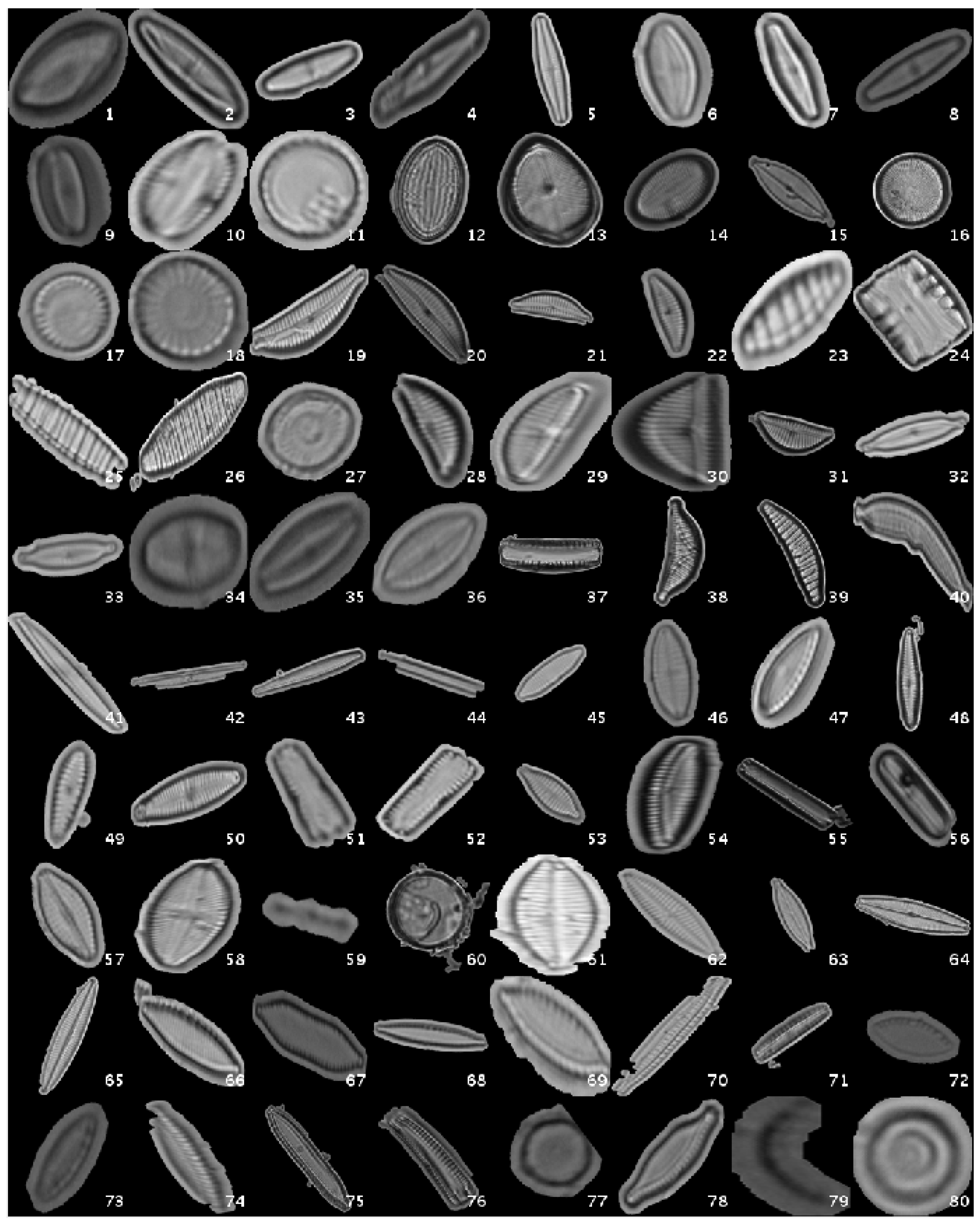
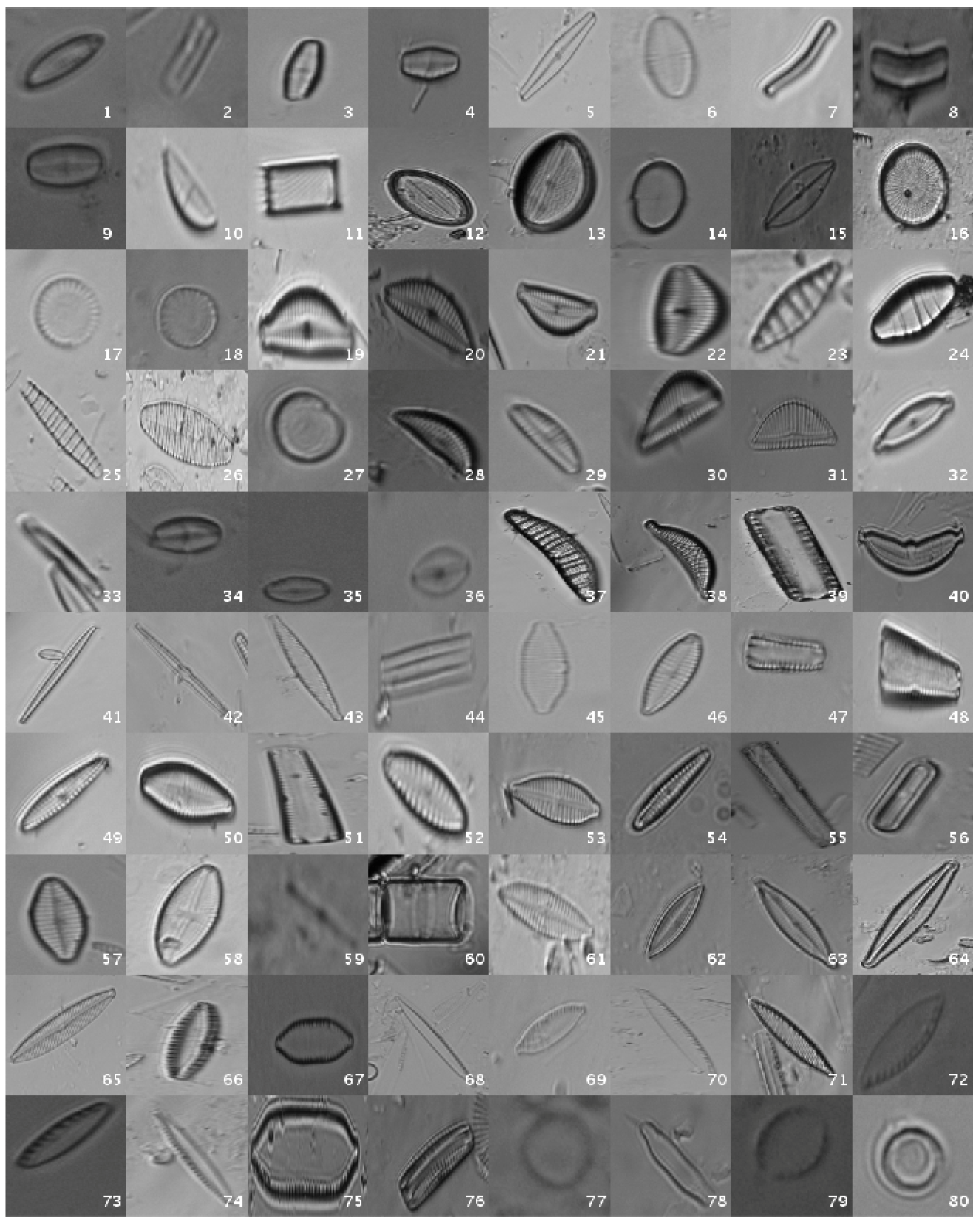
This original dataset contains sample images without applying any kind of processing, i.e., the diatoms as acquired by the expert.
Figure 1 shows a mosaic with one image sample per species.
In order to study the influence of image contrast, background, histograms and heterogeneity, some additional datasets have been built from this original one, applying different image processing techniques.
2.4.1. Segmented Dataset
One of the traditional image processing techniques that is usually applied is segmentation, in which only the interesting object in the image is conserved, turning the rest of it into black, applying some kind of mask. The exact method that was used to develop this dataset is described in the previous article from this issue [
4]. In summary, the segmentation is done by means of a binary thresholding where the segmented region are binary masks where descriptors must be computed.
The process to obtain the binary masks consists of four steps:
Binary Thresholding: automatic segmentation based on Otsu’s thresholding.
Maximum area: calculation of the largest region (area).
Hole filling: interior holes are filled if present.
Segmentation: the ROI is cropped with the coordinates of the bounding-box of the largest area (step 2).
Figure 2 shows a mosaic with one image sample per species.
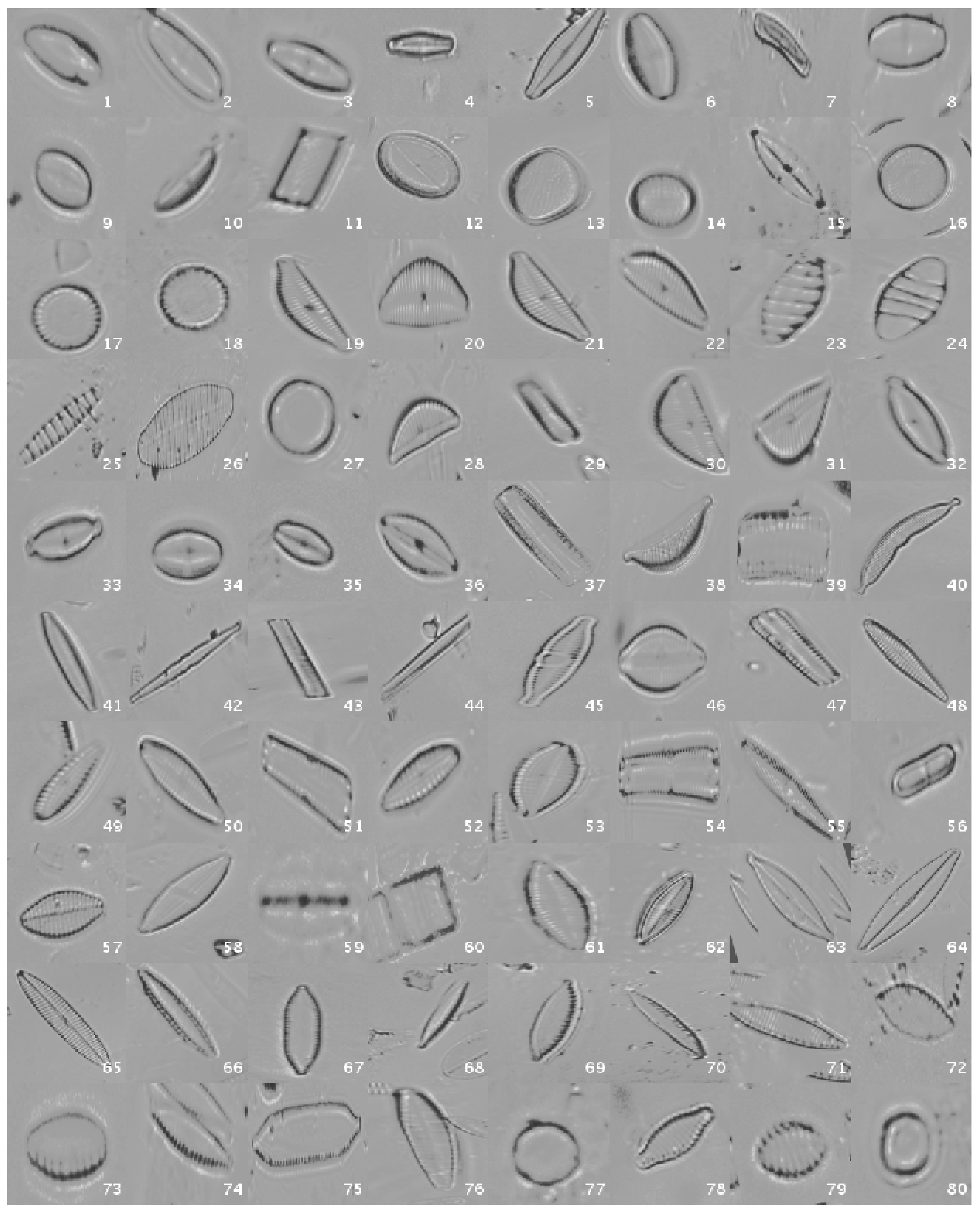
2.4.2. Normalized Dataset
In order to study whether different image contrast and illumination conditions among the species may affect learnings and discriminations, a global normalization is applied to obtain a new dataset. The technique that has been employed is histogram matching, described in [
11]. The fundamental of this process is to select a reference image, with good contrast and definition, and fit the histogram of the rest of images to that one.
The technique follows this process: the histograms of the reference R and target T images are computed. After that, the cumulative distribution functions (F) of those histograms are calculated. Using that information, the goal is to determine which grey level () in the target image fulfills that (). This is applied to every single pixel in target images.
Figure 3 shows a mosaic with one image sample per species.
2.4.3. Original + Normalized Dataset
Finally, an heterogenous dataset is built. In this case, the images from original and normalized datasets are merged, so that this dataset would be useful to study whether the variety of image sources and features contributes to the accuracy in the classification process.
3. Deep Learning
The approach is based on applying the CNN paradigm to the different datasets that have been generated. First of all, a general overview is provided. After that, the specific details about training, testing and validation processes are explained.
3.1. Convolutional Neural Networks
CNNs are based on simple neural networks, with some additional features. These are mainly new ways of organizing and applying the neurons to the data. Numerical parameters rule the learning process and its tuning can be crucial to obtain good results.
The network is fed with every single sample and the answer the net provides is improved applying several iterations, making it closer to the expected answer minimizing the loss function. The exact mathematical mechanisms to solve this problem are the so-called
solvers. Among them, Stochastic Gradient Descent (SGD), is the basis and the most common, but there also are important variants like Adaptive Gradient (AdaGrad) presented in [
12] or Nesterov Accelerated Gradient (NAG) introduced in [
13].
3.2. Training
The method that has been developed takes advantage of a transfer learning technique called fine-tuning. That is, taking a previously trained model that has learned good general features and apply that to our own dataset, adapting the network weights for the problem at hand. The model used was a pretrained AlexNet model from the ImageNet challenge (see [
6]). Given that, it was possible to achieve good results with only a few epochs/iterations.
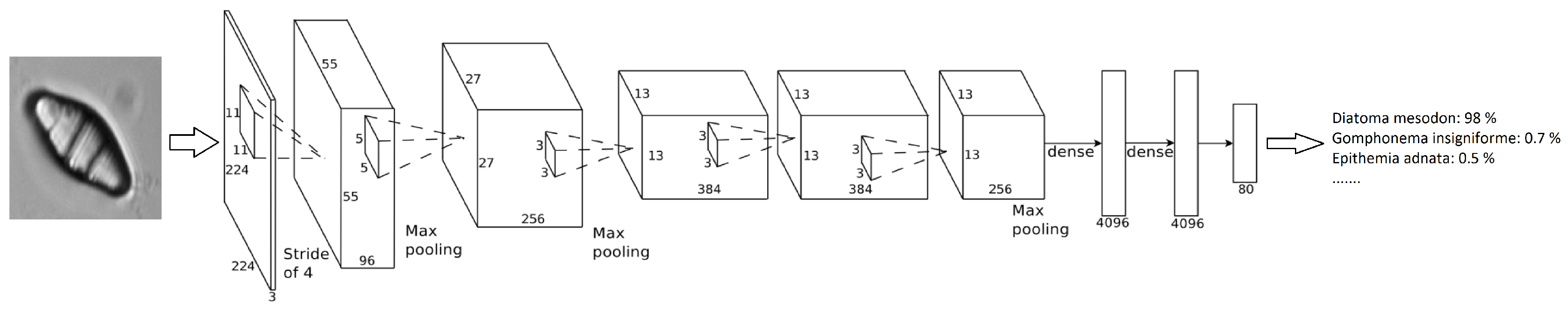
Figure 4 shows how this network is organized, an input image is provided and, after the neuronal activations throughout the layers, a percentage of confidence in the decision class is provided. In
Table 3, the architecture layers are presented in detail.
The training process is started out with an initial learning rate of 0.001, decreasing it with a drop factor of 0.1 with a period of 8. For back propagation, the Stochastic Gradient Descent was used, establishing 0.004 for L2-Regularization. With the previous parameters, training reaches the best results with just 10 epochs (after that number the loss value and accuracy do not improve). It takes around 1 h to perform a training process (i.e., training one fold of cross-validation), using the GPU NVIDIA GTX 960 Ti with 6 GB of VRAM. To perform the experiments, 10 fold cross-validation has been applied, with 9 folds for training and the remaining one in each iteration for testing.
As described in the publication of the architecture that is employed in this work ([
6]), there are two techniques that this method applies to face overfitting, one of the major problems of Deep Learning. The first one is data-augmentation, since the application of rotations and reflections over the input images ensures that different versions of the same samples are provided, so that the features the model learns are more general. The other one is the use of dropout layers in the architectures (which are present in the model that is employed). The idea is to randomly “turn off” some of the neurons, so local dependencies throughout the network are avoided, making the model more robust.
3.3. Testing
Taking the 10% of the dataset that was reserved for testing in each fold, the trained model was applied to these images, classifying each one individually and calculating the resulting confusion matrix. Using the hardware described above, it takes around 0.007 s to classify a single image.
3.4. Validation
Once any image analysis method has been applied, it is important to quantify the performance to know how accurate it is or compare it with other methods. The most widely used technique to measure the behavior of a classifier is the
Confusion Matrix. T. Fawcett performs a comprehensive review of this topic in [
14]. Here, the most important concepts are summarized.
The Confusion Matrix is a tabular representation which states the relationship between the predicted instances and the correct results. This way, there are four kinds of items:
True Positive. The instance belongs to the class and so is predicted.
False Positive. The instance does not belong to the class but is predicted as positive. This is the so-called Type I error.
True Negative. The instance does not belong to the class and so is predicted.
False Negative. The instance does belong to the class but is predicted as negative. This is the so-called Type II error.
From this matrix, some metrics can be calculated to summarize the performance in certain aspects. The most important ones are:
True Positive Rate (TPR) or Sensitivity. Defined in Equation (
1), it measures the proportion of positive samples correctly classified.
True Negative Rate (TNR) or Specificity. Defined in Equation (
2), it measures the proportion of negative samples correctly classified.
Accuracy. Defined in Equation (
3), it measures the proportion of correctly classified samples (positives and negatives) against the total population (number of samples that have been classified).
4. Results and Discussion
Using the datasets and the method introduced in the previous section, some experiments have been performed, varying the number of samples for training and applying cross-validation to check the performance of convolutional neural networks in this problem. Hence, the training is based on using the same number of samples per species throughout the 80 classes, so the experiments are balanced. The decision is to set those values at 300, 700 and 1000 samples per species. When more samples were needed, some extra rotation with fewer degrees step gap (typically 2) were applied.
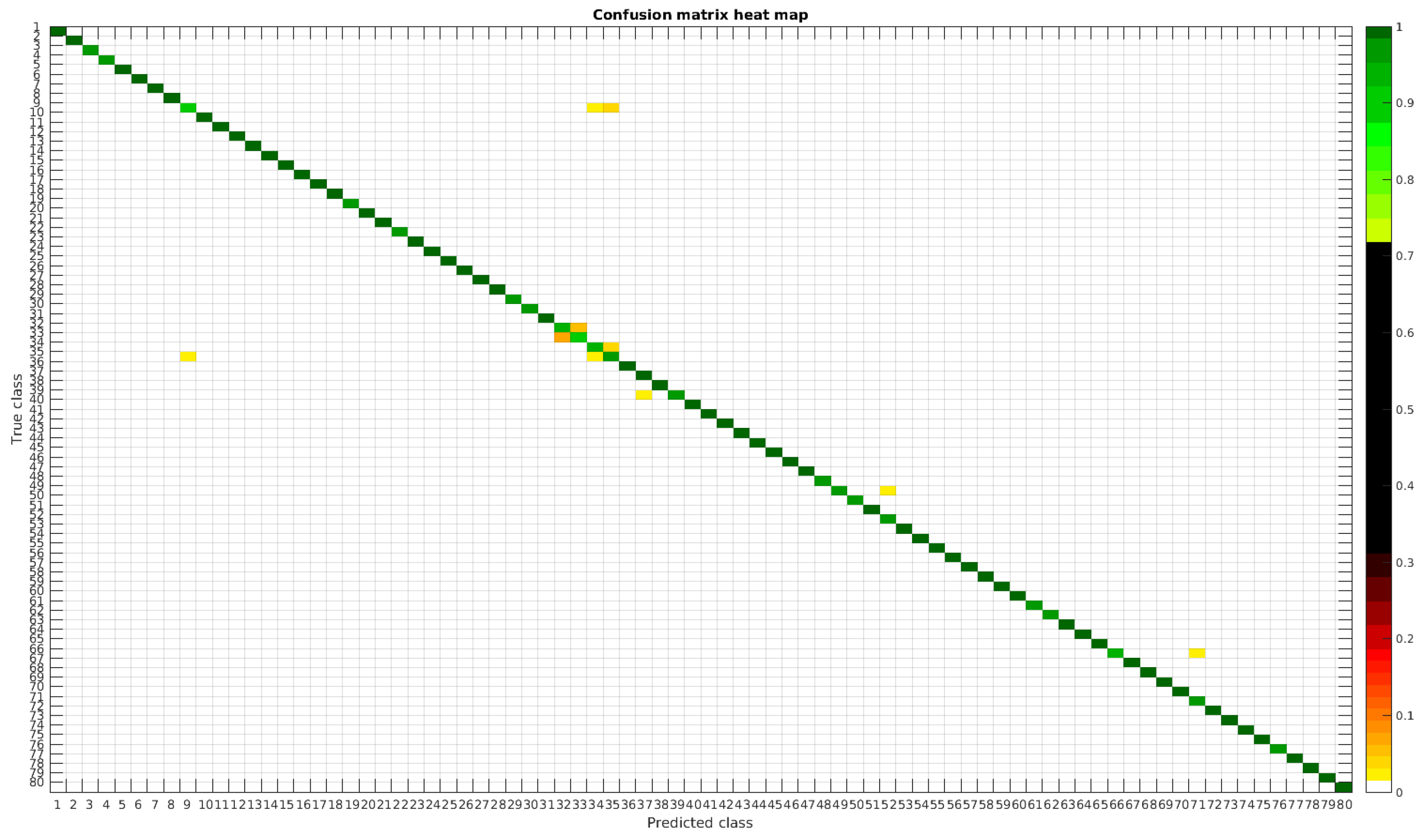
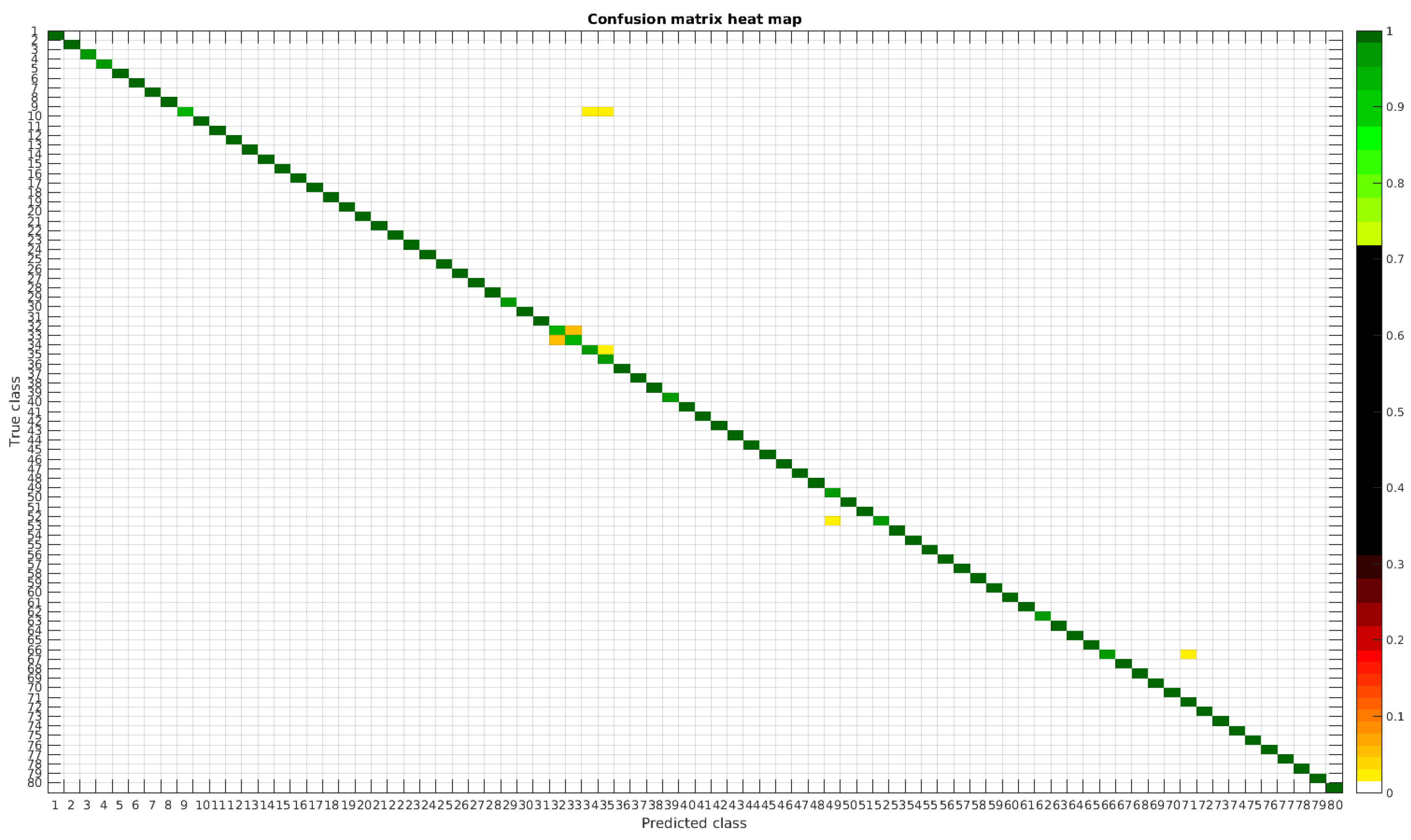
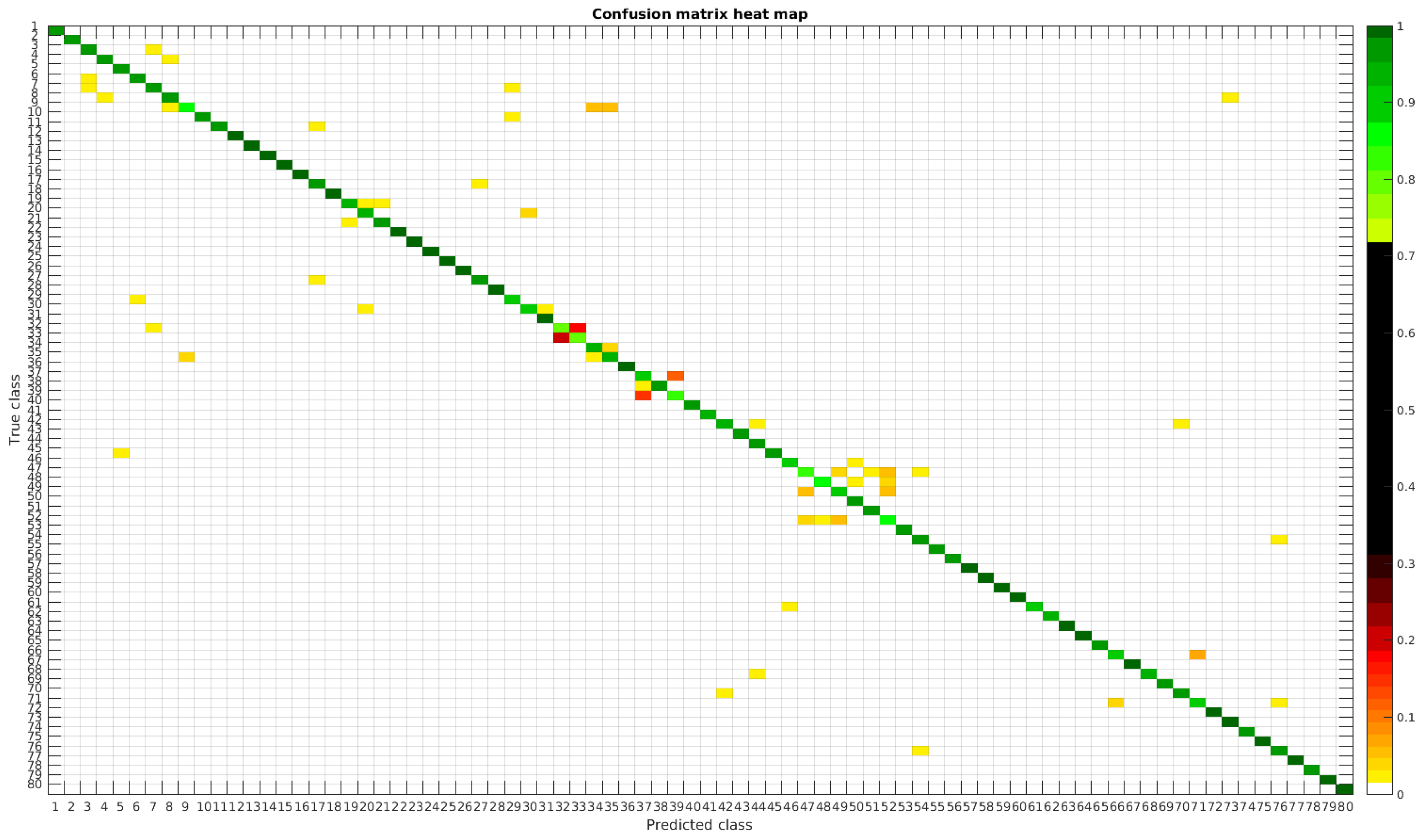
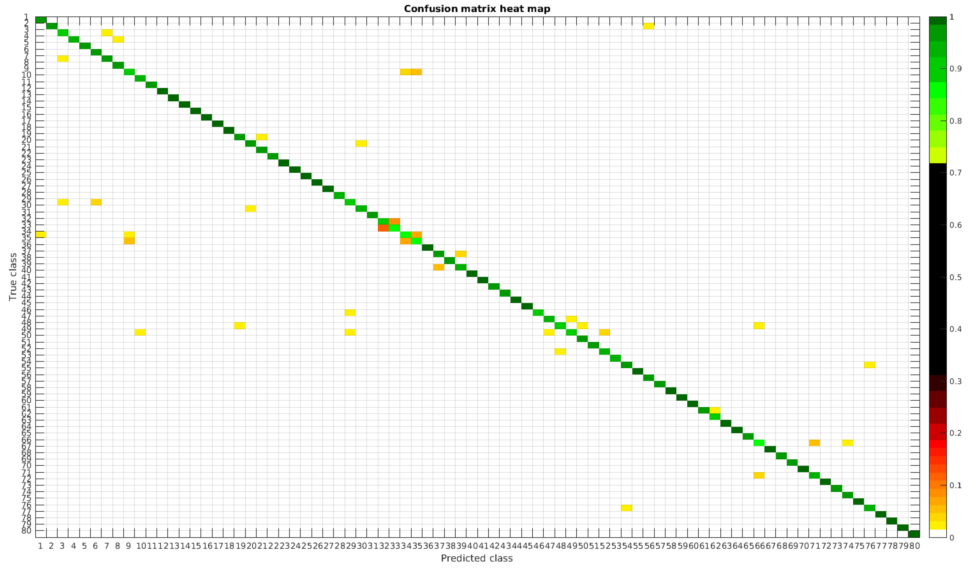
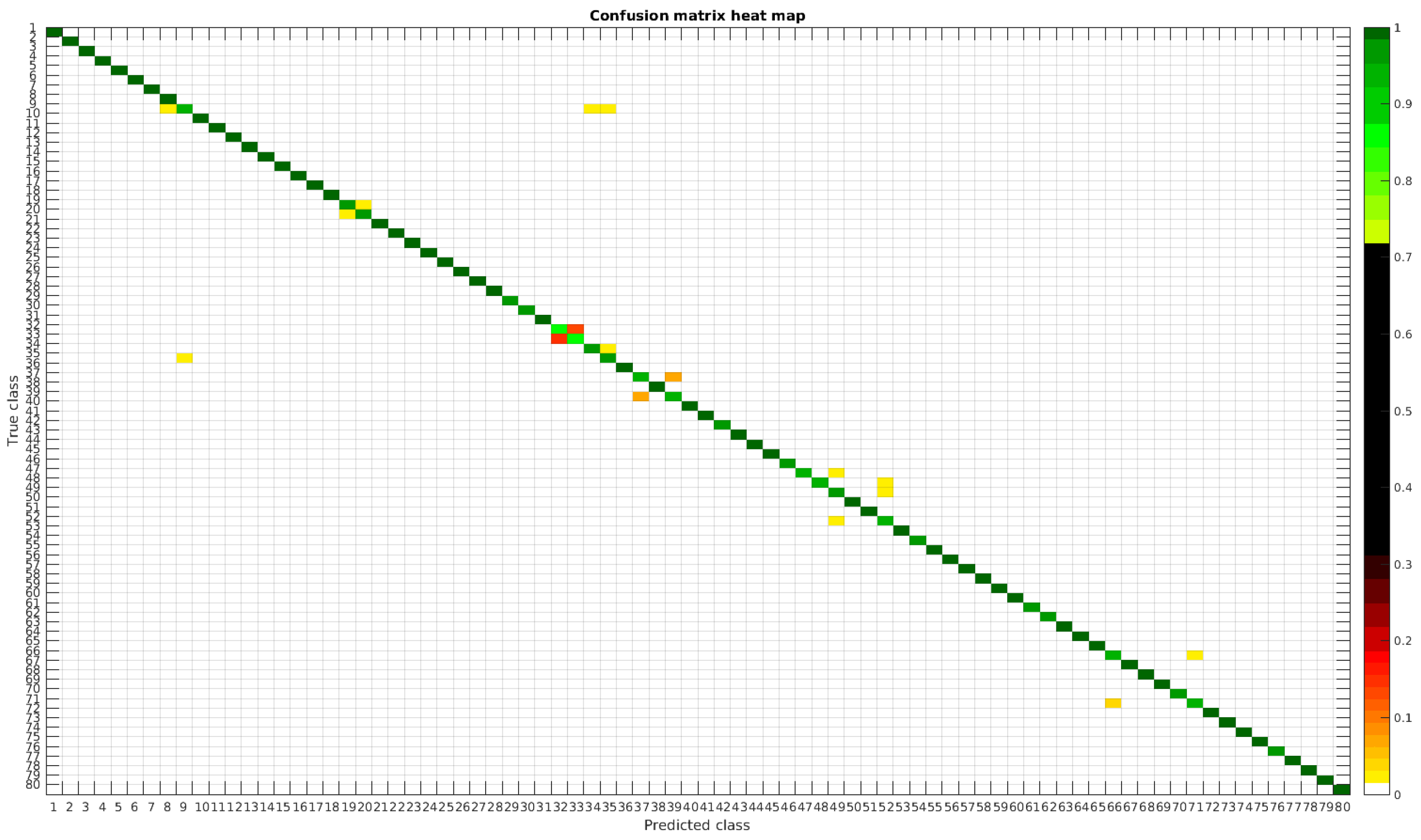
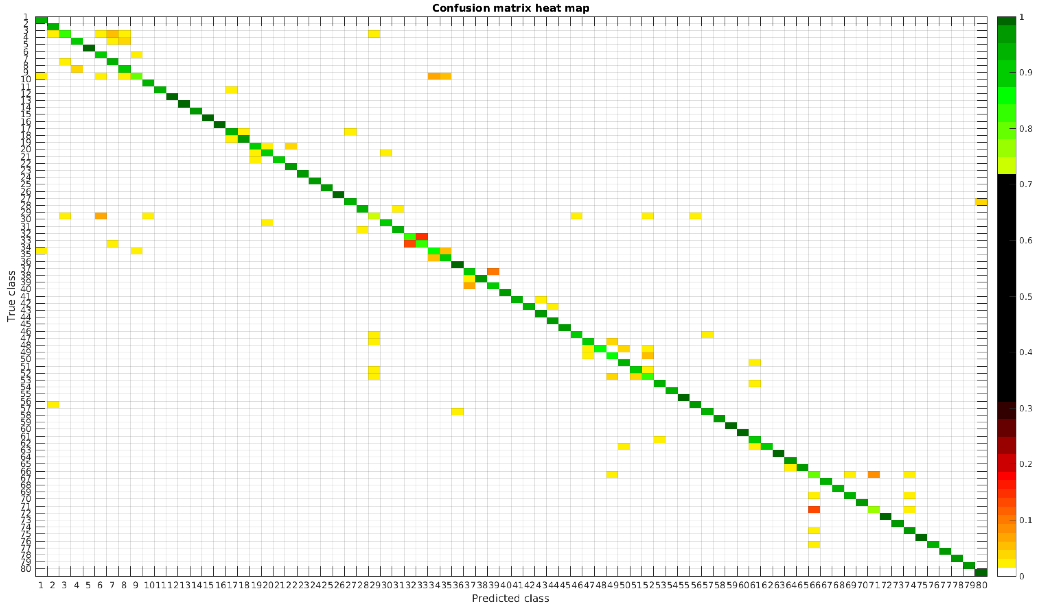
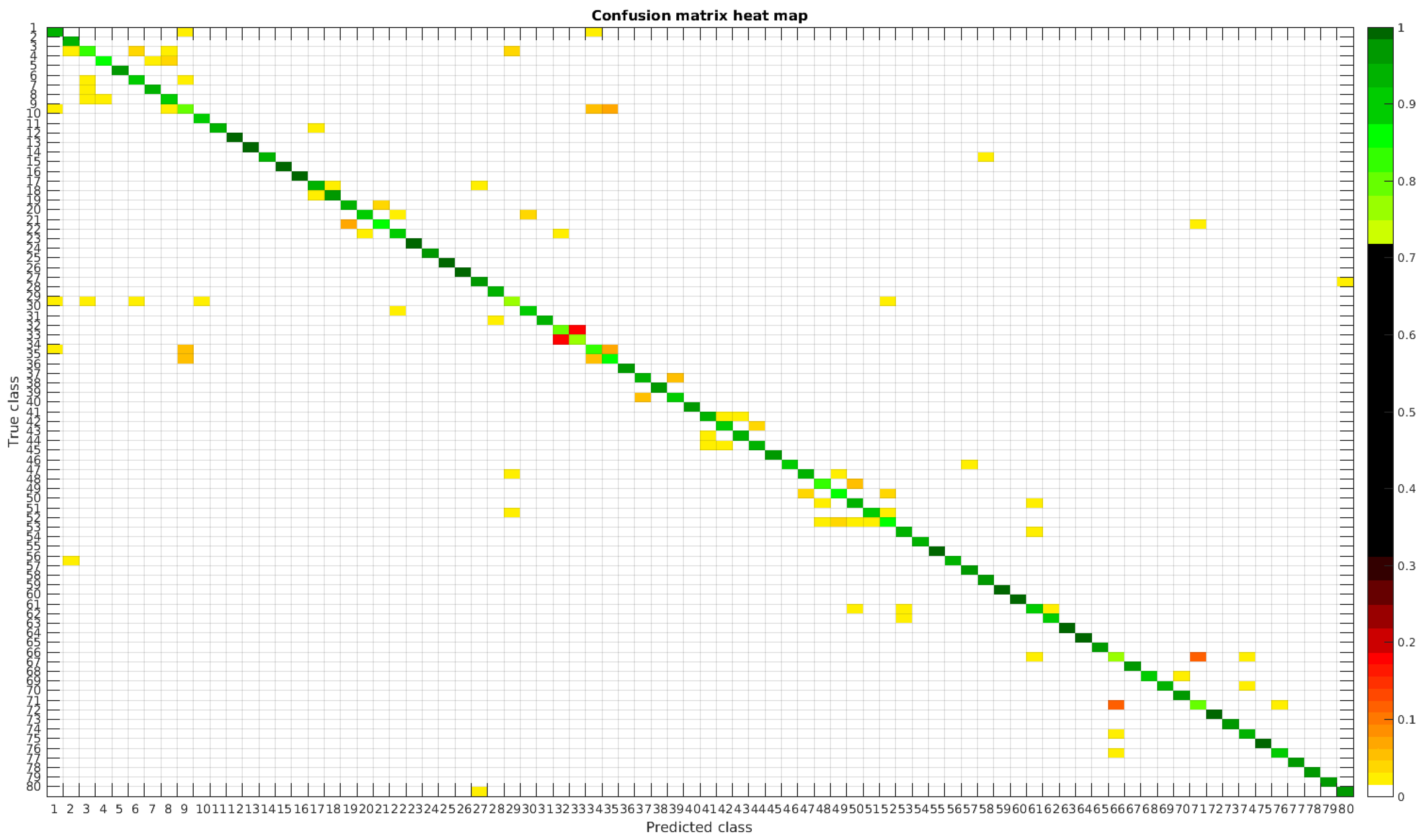
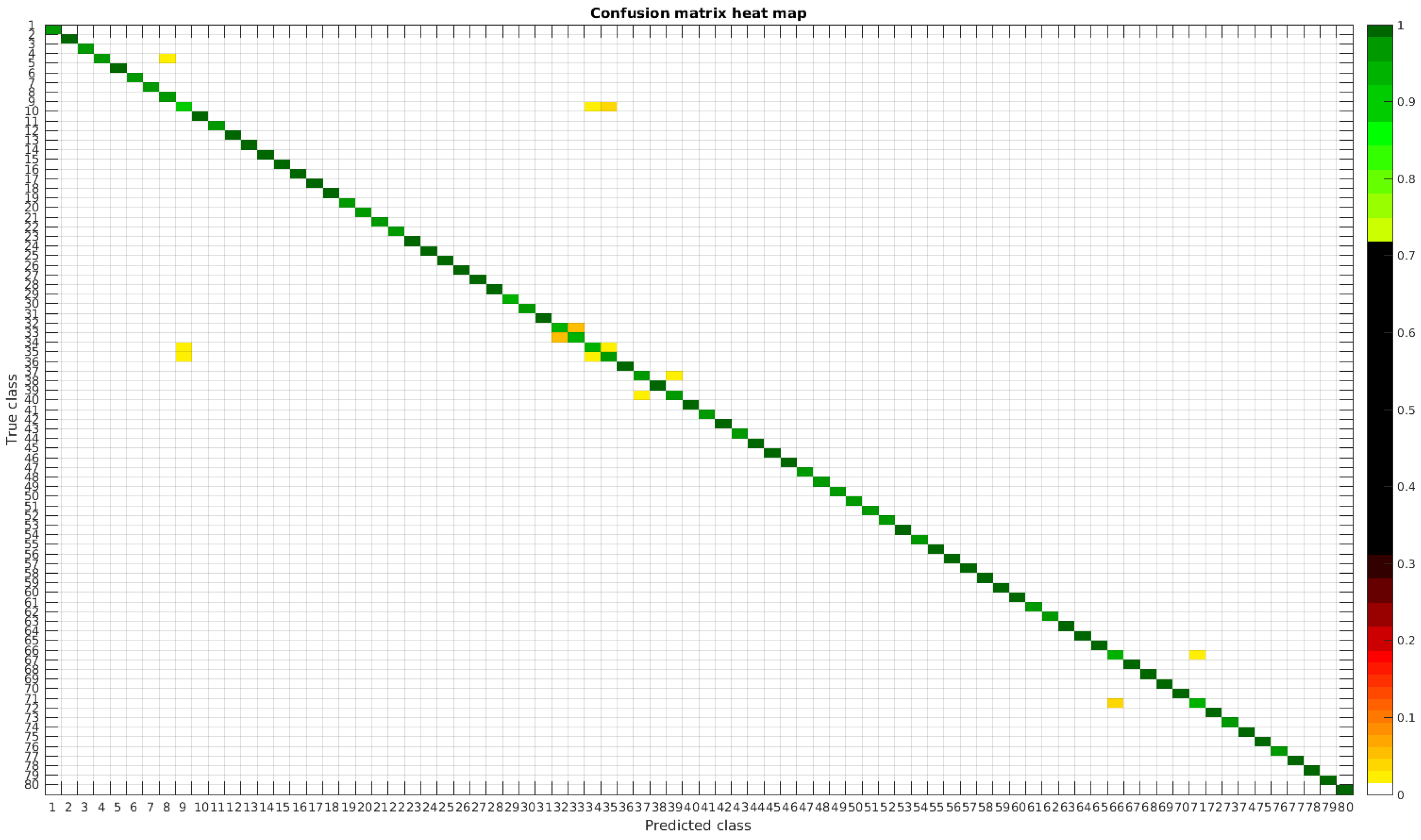
The results are illustrated using a heat map representation of the confusion matrices. The colorbar means the percentage of images (between 0 and 1) from a given class (row) that has been classified as the species in the corresponding column.
4.1. Original Dataset
The confusion matrices for training with 300, 700 and 1000 samples per class are presented in
Figure 5,
Figure 6 and
Figure 7 respectively.
Table 4 shows a summary of experiments with the original database, giving precise information about the dataset, the number of samples per class, the mean accuracy of the 10 folds from cross-validation and standard deviation. The accuracy for testing has been calculated as the percentage of labels that match between the ground truth and the classifier. Notice that when the number of samples per species is increased, the accuracy is improved and only some of the confusions remain.
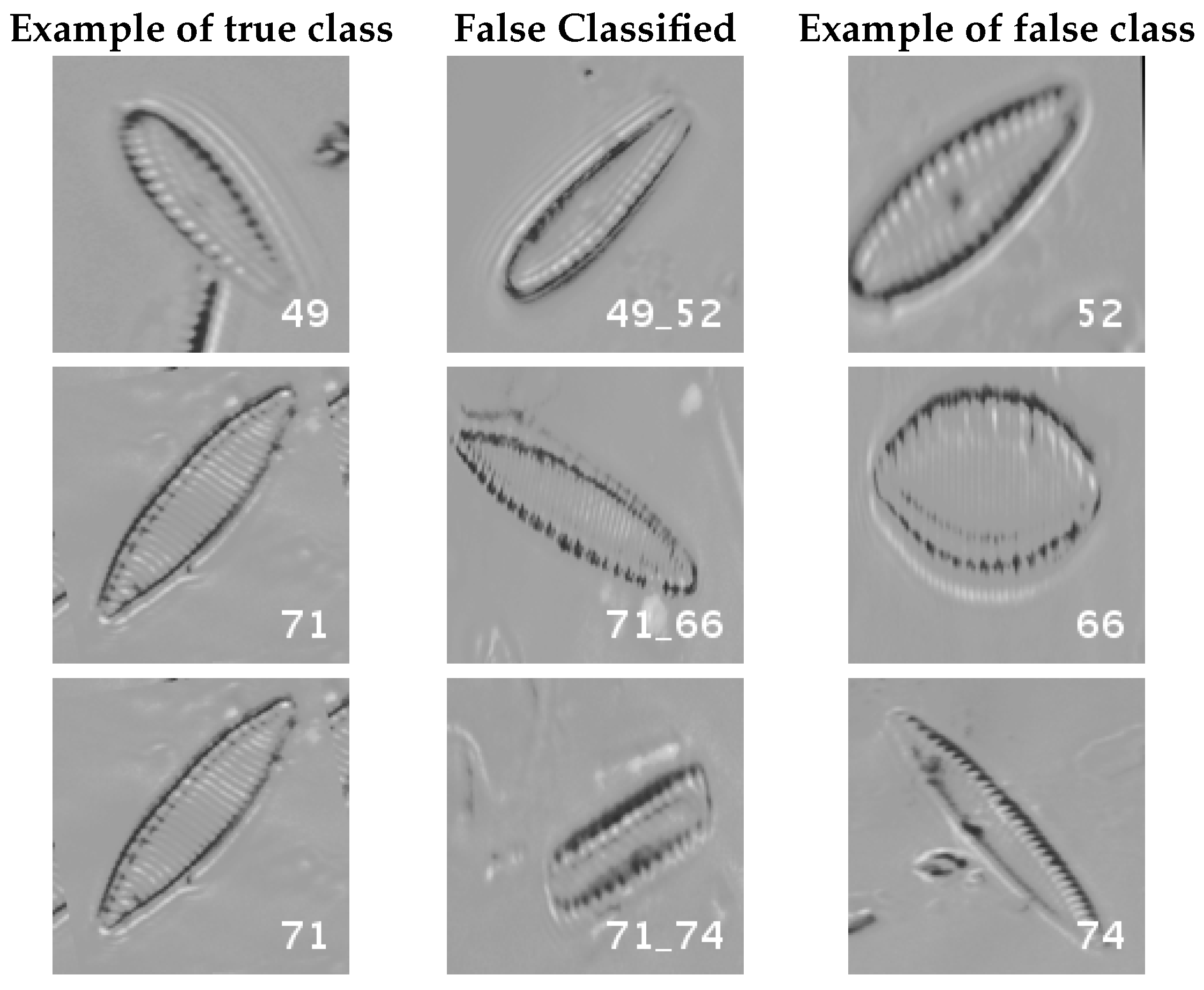
In
Figure 8, a summary of the most frequent confusions is shown, where, the first row shows a confusion between
Achnanthidium caravelense (3) and
Achnanthidium exile (7). Further than belonging to the same family, the confusion is most likely to be produced because of the presence of “valve view” (the view of the frustule when the valve is uppermost) and “girdle view” (the view of the frustule when the girdle is uppermost) samples in the dataset, the latter being much more difficult to be distinguished from each other. A similar appearance of the images would be the most common source of confusions throughout the different experiments.
The diatom species that show initially a larger error are: Encyonopsis alpina (32), Encyonopsis minuta (33), Eolimna minima (34) and Eolimna rhombelliptica (35).
4.2. Segmented Dataset
Using the segmented dataset, the same experiments were performed. The confusion matrices for training with 300, 700 and 1000 samples per class are presented in
Figure 9,
Figure 10 and
Figure 11, respectively.
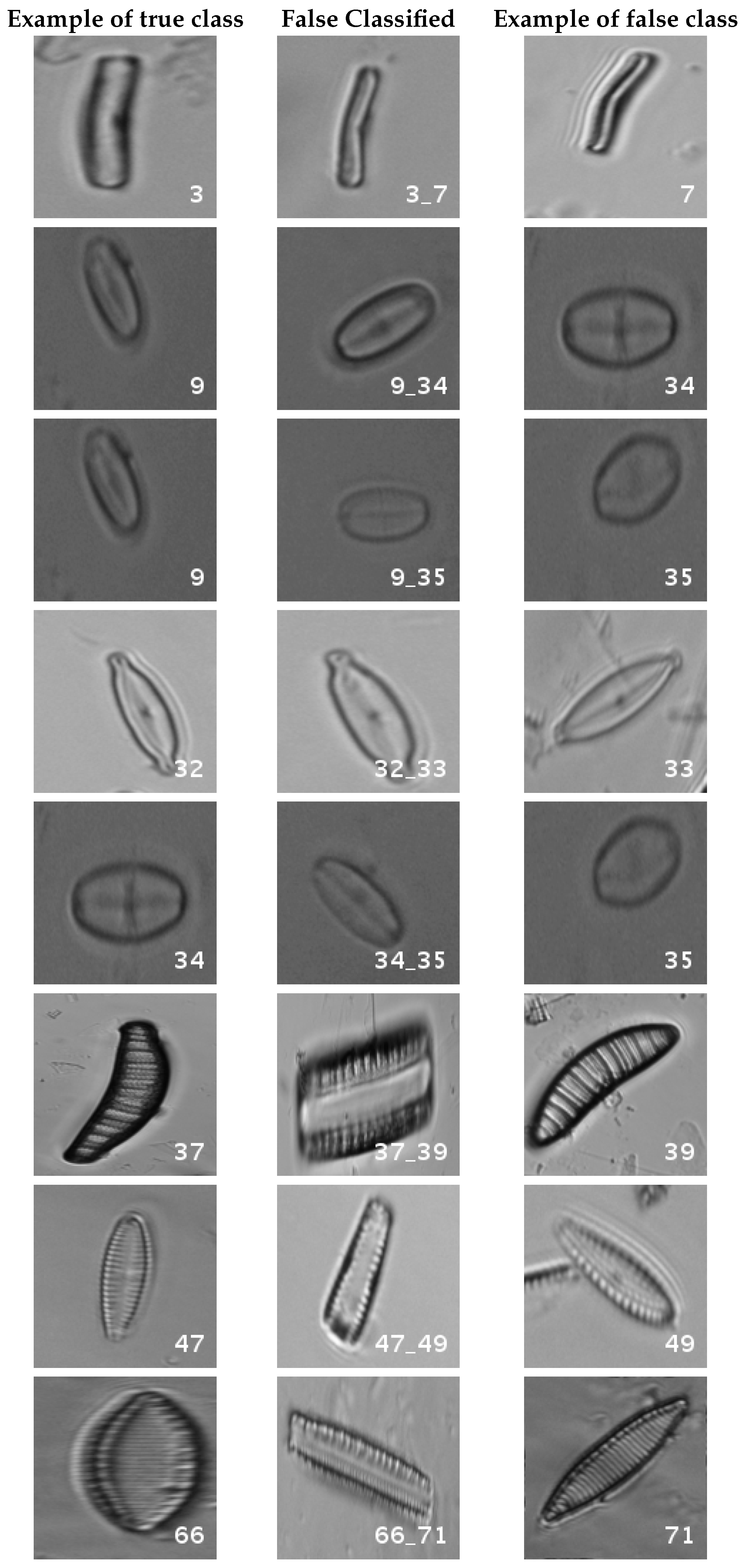
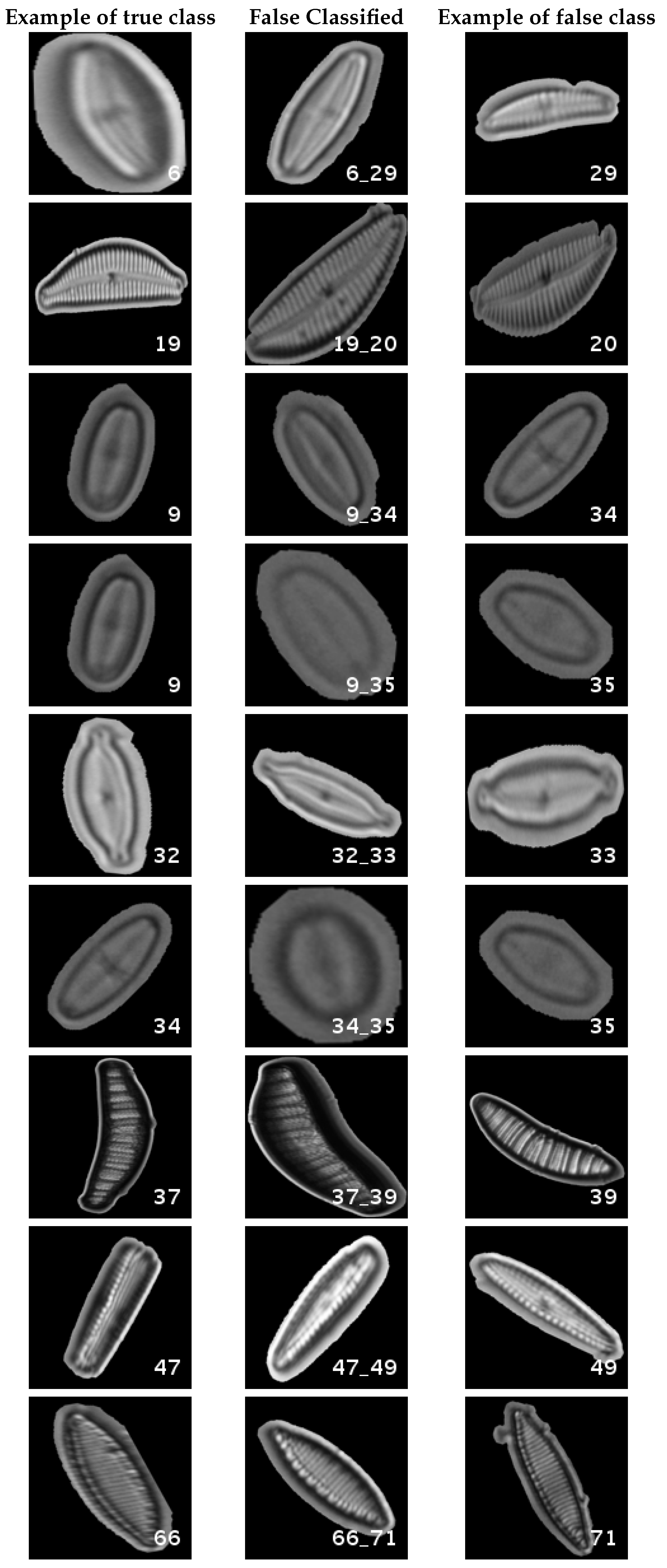
In
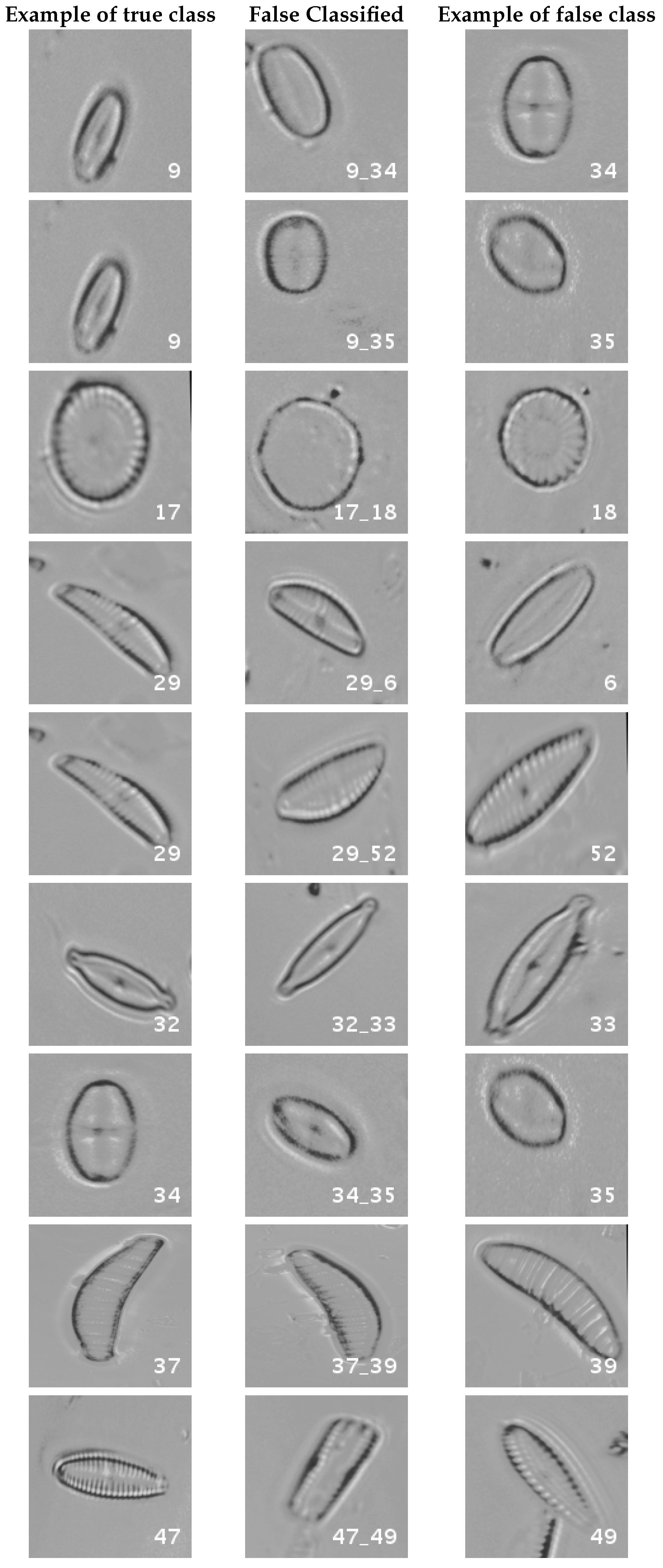
Figure 12, a summary of the most frequent confusions is shown.
In this dataset, again, the majority of bad classifications are due to species that are quite similar to each other. However, in comparison with the previous dataset, there are more pairs of species that maintain a (relatively) significant error rate. These are:
- -
Cymbella excisa var angusta (19) and Cymbella excisa var excisa (20);
- -
Encyonopsis alpina (32) and Encyonopsis minuta (33)—same than the original database;
- -
Eolimna minima (34) and Eolimna rhombelliptica (35) —same than the original database;
- -
Epithemia adnata (37) and Epithemia turgida (39);
- -
Nitzschia amphibia (66) and Nitzschia fossilis (71).
Once again as the number of training samples per species is increased, the accuracy improves, and most of the confusions disappear.
Table 5 shows a summary of the experiments with the segmented database. Notice that this database is the same that the one used in the previous article [
4]. The handcrafted approach based on bagging tree performs better for lower number of samples, that is for 300 samples per class the overall accuracy was 98.11% versus the current 95.62% with CNN. The result, as compared with classical handcrafted approaches only improves when the database is larger than 700 samples per class.
4.3. Normalized Dataset
The confusion matrices for training with 300, 700 and 1000 samples per class are presented in
Figure 13,
Figure 14 and
Figure 15, respectively.
In this dataset, apart from some pairs of species that are usually confused, there are some of them which are confused with more than 2, 3 or 4 species equally. Moreover, the number of misclassified classes is higher than the previous experiments when the number of samples per species is reduced. However this is quickly reduced when the number of samples per class is increased to 1000, reaching then similar accuracy values.
Table 6 shows these results with the normalized database.
The following list stated some species that are misclassified and the respective species with whom they are confused:
- -
Encyonema reichardtii (29): Achnanthidium atomoides (2), Achnanthidium caravelense (3), Achnanthidium eutrophilum (6), Gomphonema minutum (52).
- -
Achnanthidium rivulare (9): Achnanthes subhudsonis (1), Achnanthidium atomoides (2), Achnanthidium eutrophilum (6), Eolimna minima (34), Eolimna rhombelliptica (35).
- -
Nitzschia fossilis (71): Nitzschia amphibia (66), Nitzschia tropica (74).
Even though the images are slightly different compared to the previous datasets, the classes that are more difficult to classify are similar. Finally, when the number of samples per species is over 1000, only two pairs of diatoms have some perceptible error. They are:
- -
Encyonema alpina (32) with Encyonopsis minuta (33).
- -
Nitzschia amphibia (66) with Nitzschia fossilis (71).
Figure 16 and
Figure 17 show a summary of the most frequently pairs of species that are misclassified as mentioned above.
4.4. Original + Normalized Dataset
This dataset, as it was explained, is proposed to determine whether a combination of images with different preprocessing can make the model more robust. The results states that this has some impact, but the main weight in accuracy still depends heavily on the number of samples. When the balanced training process has 1000 samples per class, similar values in accuracy are obtained, and this value is even increased when 2000 samples are used.
In terms of misclassified species, this dataset behaves in the same way as the rest, stating that even with images from different sources in terms of different processing techniques the learned model is not affected, making it quite robust in comparison with other methods.
Table 7 shows a summary of the experiments done with this database, giving precise information about the dataset, the number of samples per class, the mean accuracy of the 10 folds from cross-validation and standard deviation. The accuracy for testing has been calculated as the percentage of labels that match between the ground truth and the classifier. Additionally,
Table 8 show the top-30 species that are missclassified, with the sensitivity achieved with this model.
4.5. Discussion
From the results, it is clear that accuracy is increased (and the standard deviation is decreased) when the number of training samples increases. This behavior is one of the greatest advantages of deep learning, since traditional machine learning techniques are less likely to increase their accuracy when the dataset is enlarged. It is worth noting that results improve compared to handcrafted methods when the number of samples exceeds 700 samples per class. Otherwise, the combination of several features based on morphological and textural properties may performs better with decision trees classifier than the CNN as shown in the previous study [
4] (see
Section 4.2).
It has been observed that, apart from the intra-dataset relation among the species that perform worse, this relation is kept inter-datasets. As a result, whichever dataset and number species for training, the species that are more difficult to be classified for CNNs are: Encyonopsis alpina (32), Encyonopsis minuta (33), Epithemia adnata (37) and Epithemia turgida (39).
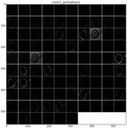
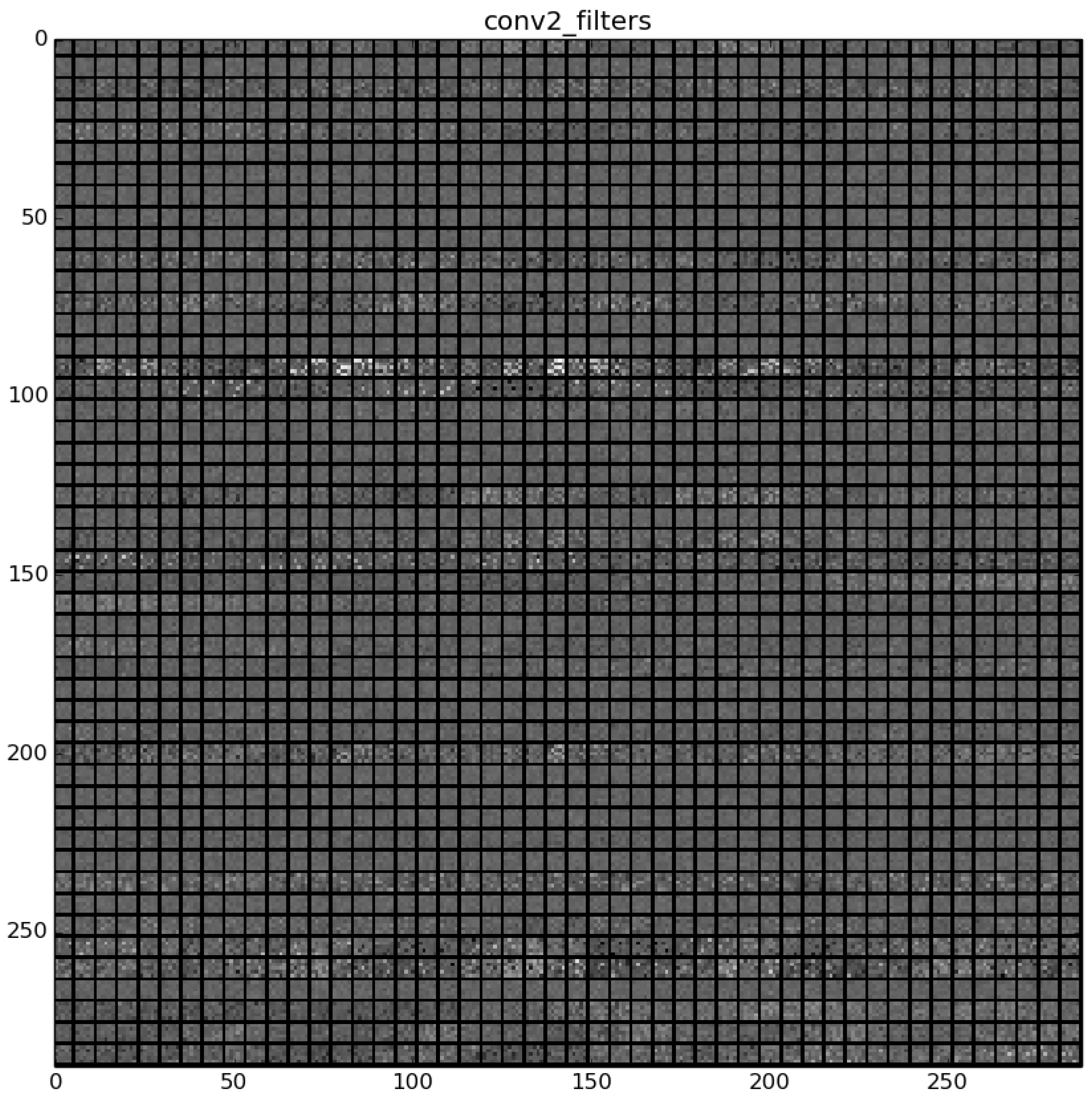
Finally, when convolutional neural networks are applied, it is suitable to show how the filters that contain the learned features look like, as well as the activations that are produced with a given example.
The learned features of a CNN model are stored in the weights of its layers, being the convolutions the most significant ones. The illustration will be limited to convolution 1 and convolution 2 layers, as they are the most significant ones to be visualized.
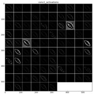
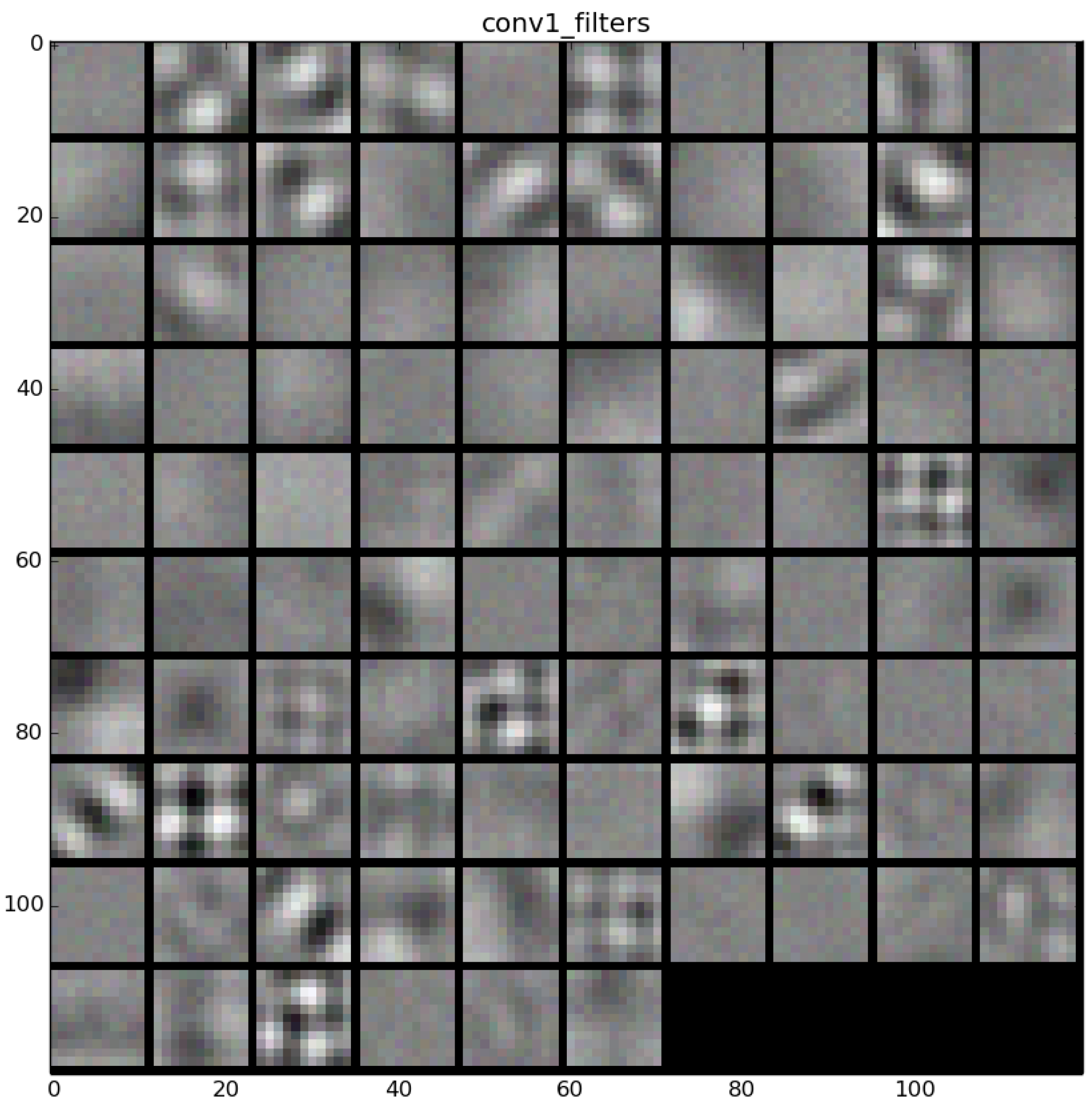
Figure 22 shows the learned filters in the convolution layer 1 of AlexNet. Attending the layer size, there are a total of 96 different filters (as it is observed in the matrix of patches), with 11×11 pixels size each. As a result, when a sample is fed throughout this layer, these filters are applied directly over the input image and each of them produce a different result, as shown in the second column of
Table 9.
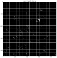
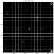
Figure 23 shows a visualization of the weights in convolution layer 2. The structure of the layer is more complex (and so on happens when we go deeper in CNN layers). This layer has filters of 48×48 channels with 5×5 pixels size each. In the image, each of these channels is shown in a single patch. This layer has a total of 256 filters, so this is the number of output patches that are obtained when these filters are applied over the results of the previous layers, as it is observed in the third column of
Table 9.
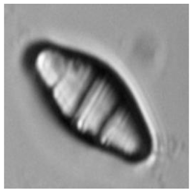
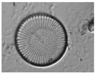
As mentioned before,
Table 9 shows two examples of diatoms from
Diatoma mesodon and
Cyclostephanos dubius respectively, and their corresponding activations for convolution 1 and convolution 2 layers.
5. Conclusions
In this paper, the whole workflow of an image classification process with CNN has been covered: from dataset building, classification and results interpretation. The application of CNN to the problem of diatom classification has shown up some interesting conclusions, such as its invariance to image from different processing techniques. Hence, regarding the hypothesis that was stated about the influence of image contrast and illumination conditions on learning and discrimination, it has been proven that the results are similar regardless of the database used. Moreover, the species with larger error are usually the same. The misclassified sample is usually produced because of the presence of different views, “valve view” and “girdle view” for the same diatom type.
As far as the authors know, this is the first time that CNN has been applied to diatom classification. The applied methodology shows that the classification of large numbers of diatom species can be tackled with CNN always assuming that a large database can be provided. In our experiments with 2000 samples per class, i.e., 160,000 samples in total, an overall accuracy of 99.51% was obtained. Since CNN models take advantage from GPU computing for training but for testing too, the running time overcomes other methods, being able to process ten thousand of images in around a minute, as stated in
Section 3.3.
Regarding future work, a step further would be to achieve not only classification but detection too. This way, the method would be available to determine the diatom position and species over a Whole Slide Image (WSI), so, this way, labeling and a biologist expert would not be necessary except for checking and application purposes. This can be achieved for example, using Region-based Convolutional Neural Networks (R-CNNs), or, by applying sliding windows over the image, classifying individual patches with a previously trained CNN.


 ,
, 


