Abstract
Software defined network (SDN) is a new network architecture in which the control function is decoupled from the data forwarding plane, that is attracting wide attentions from both research and industry sectors. However, SDN still faces the energy waste problem as do traditional networks. At present, research on energy saving in SDN is mainly focused on the static optimization of the network with zero load when new traffic arrives, changing the transmission path of the uncompleted traffic which arrived before the optimization, possibly resulting in route oscillation and other deleterious effects. To avoid this, a dynamical energy saving optimization scheme in which the paths of the uncompleted flows will not be changed when new traffic arrives is designed. To find the optimal solution for energy saving, the problem is modeled as a mixed integer linear programming (MILP) problem. As the high complexity of the problem prohibits the optimal solution, an improved heuristic routing algorithm called improved constant weight greedy algorithm (ICWGA) is proposed to find a sub-optimal solution. Simulation results show that the energy saving capacity of ICWGA is close to that of the optimal solution, offering desirable improvement in the energy efficiency of the network.
1. Introduction
Since McKeown et al. proposed OpenFlow in 2008 [1], the concept of software defined network (SDN) has gradually rooted in the network field. Different from traditional networks, SDN moves the control function from the data forwarding devices to a centralized control plane, simplifying data forwarding devices and providing more flexibility and controllability to the network administrators. In the centralized control plane, one or more controllers manage the traffic flow according to the global view of the network, providing a higher capability for handling network problems. In this paper, we mainly focus on the energy waste problem in SDN.
As reported in [2], the energy consumption of information and communication technologies (ICT) were responsible for more than 8% of the global electricity consumption in 2008. Furthermore, it has been predicted that this percentage will increase dramatically in future years. Under such high energy consumption, the efficiency of the network energy is very low, which results in a serious energy waste problem. Generally, networks are always designed to satisfy the peak periods of the network traffic. However, for most of the time, the traffic load of the network is far below that in peak periods. This causes underutilization of the network devices. For example, in the previous network of Google, the average utilization of all the links was 30∼40% [3]. Yet the energy consumption of the devices in low utilization periods is almost as same as that in heavy load periods [4], resulting in low energy efficiency of the network devices. It is of great importance to improve the energy efficiency of the network, both for reducing the operation cost of internet service provider (ISP) and for environment pollution reasons.
Much research has studied the energy waste problem from different network levels. For both wireless networks and core wired networks, a common way to reduce energy waste is by putting the idle devices into low-power sleep mode or switching them off when in low traffic periods. For example, in [5,6], the authors propose a switch on/off algorithm to improve the energy efficiency of the base stations in LTE-Advanced networks. The work in [7,8] considers the problem in general cellular networks, and addresses the problem on the premise of switching off base stations. Reference [9] works on the energy saving problem in heterogeneous networks based on the switch off strategy.
For core wired networks, instead of base stations, the devices such as routers and switches (or parts of them, such as ports) are considered to turn to sleep mode for energy saving. In [10], sleeping methods are divided into two categories, uncoordinated sleeping and coordinated sleeping. Uncoordinated sleeping refers to systems where network devices determine whether turn to sleep according to their own respective status. In coordinated sleeping which devices turn to sleep is determined by all the network devices jointly, routing the traffic on part of the devices according to the current traffic load, and sleeping the idle part. Obviously, in regard to the ability of saving energy coordinated sleeping performs better than uncoordinated sleeping. Much research such as [4,11,12] based on the premise of coordinated sleeping made efforts to improve the energy efficiency of the network. However, there are many difficulties in executing the coordinated sleeping in traditional networks. As discussed in [10], first, some network protocols must be changed. For example, the Hello message should be sent only among the active devices. Secondly, which devices should be put into sleep mode is a complicated problem for distributed control networks. Thirdly, some unexpected side effects such as route oscillation may be caused. Thanks to the centralized controller(s), in SDN coordinated sleeping will be easy to deploy without these difficulties.
At present, several works have focused on the energy waste problem in SDN based on coordinated sleeping and considered the problem from the different aspects [13,14,15,16,17,18]. The closest work to this paper is [13], where a typical architecture called ElasticTree is proposed for improving energy efficiency in SDN. The traditional energy saving strategies also can be deployed in ElasticTree to determine which devices can be shut down. While ElasticTree treats all the traffic demand as new traffic demand (as described in our previous work [14]), for energy saving, the paths of the uncompleted traffic demands generated before current optimization will be changed, which may result in route oscillation, and causes additional energy consumption for state transition. In [14], to avoid these problems, we designed a new green scheme named GreSDN for energy saving, and presented two routing algorithms that can be used in GreSDN, the constant weight greedy algorithm (CWGA) and the dynamic weight greedy algorithm (DWGA). In this extended version, with regard to the previous work [14], the main contributions of this paper are summarized as follows:
- The process of GreSDN has been improved to make GreSDN more rigorous.
- To find the optimal solution of energy saving in GreSDN, the problem is formulated as a mixed integer linear programming (MILP) problem, and the problem is found to be a NP-hard problem.
- As proved in our previous work, for the two green algorithms, CWGA performs better than DWGA in energy saving, but the computation complexity of CWGA is higher than that of DWGA. In this extended version, we further work on decreasing the computation complexity of CWGA, and the improved algorithm is named as improved constant weight greedy algorithm (ICWGA).
- In addition to studying the performance profile of ICWGA, we further examine the effect of some other factors on the performance of ICWGA, such as link density and the processing sequence of the traffic demands.
The remainder of this paper is organized as follows. In Section 2, previous energy-saving research for SDN networks is reviewed. In Section 3, we describe the green scheme and then formulate the problem in Section 4. In Section 5, the improved heuristic green routing algorithm is presented in detail. Then the performance of the green routing algorithm is evaluated through simulation in Section 6. Finally, in Section 7, we conclude the paper.
2. Related Work
At present, the energy waste problem in SDN has been considered from different aspects. In [13], Heller et al. propose an energy saving scheme called ElasticTree for software defined data center networks. An optimizer is added in the controller to calculate the devices that can be put into sleep based on the traffic load. However besides the route oscillation problem, for the TCP-based traffic, when the traffic load increases, the network capacity won’t be increased due to the adaptive congestion control of TCP, which will affect user experience as mentioned in [13].
In [16], Ruiz-Rivera et al. propose an energy saving algorithm based on the switch assignment problem. In this algorithm, controllers act as switches at the same time. Links are switched off under the condition of ensuring that all switches are connected to one controller, and all the paths satisfy delay and load constraints at the same time. A severe limitation of this algorithm is that once the links that will be shut down are determined, communication demands that can’t find a feasible path in the sub-topology will be rejected. This will affect the Quality of Service (QoS) of the network.
Giroire et al. consider the memory size of switches, modeling the energy saving problem in SDN as an integer linear programming (ILP) problem under the constraint of limiting the number of the rules in the switches [18], and propose a greedy heuristic algorithm due to the high complexity of the problem. In this heuristic algorithm, the controller routes the traffic on the switches with fewer rules through setting the link weights according to the numbers of rules in the connected switches, and determines the links that can be set to sleep mode iteratively.
In [15], the authors consider energy saving based on the controller placement problem, aiming at minimizing the energy consumption of the control network, but the energy consumption of the data forwarding plane was neglected.
Two energy-saving models are proposed for software defined data center networks in [17]. One is a 0–1 integer programming model which is a superior model for small scale networks. The other one is a greedy algorithm model which is not limited by the network scale. To find the optimal paths of energy consumption for traffic demands, the two models both need to traverse all the paths from source node to destination node of all communication pairs; this causes a lot of redundant computation.
The above works address the energy saving problem in SDN from different perspectives respectively. But as regards the energy saving problem in the data forwarding plane, most research works assume that the network is without traffic load when new traffic arrives. In our previous work [14], we proposed a real-time dynamical energy saving optimization scheme combined with routing algorithm based on the current working state of the network, and presented two routing algorithms that can be used in the scheme. In this extended version, we do a series of work to make the work more meaningful.
3. GreSDN: The Green SDN System
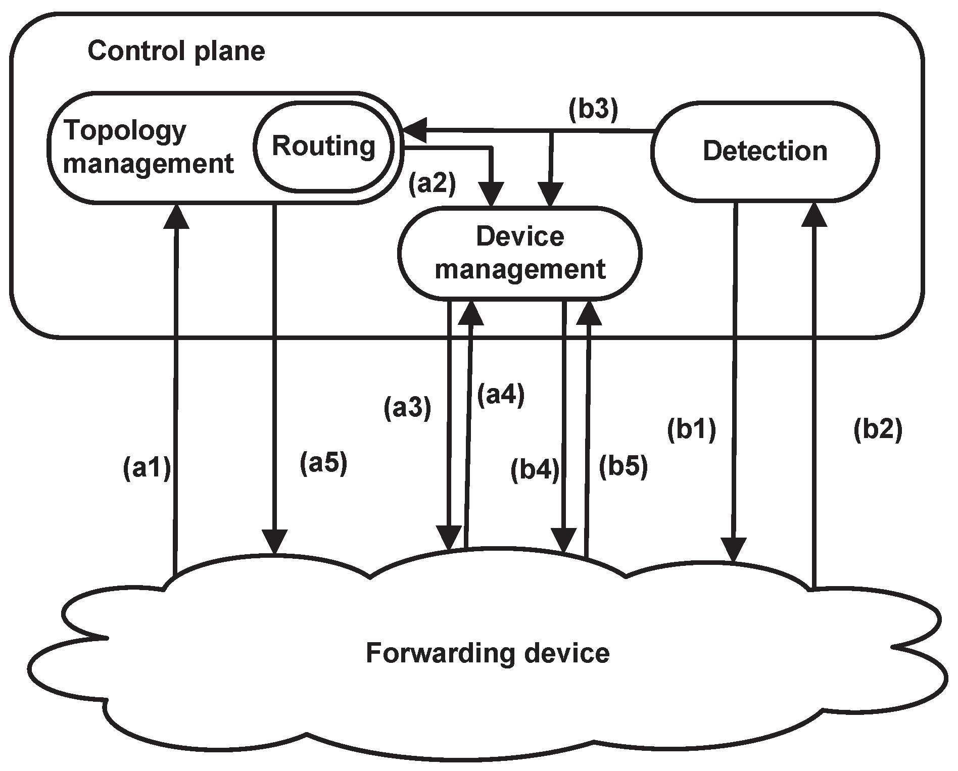
The design of the green SDN system (GreSDN) is shown in Figure 1. In the control plane, three modules are designed for the green scheme. First is the topology management module. Different from the common topology management module, the topology management module in the green scheme manages two topologies of the network. One is the real topology of network which includes all the switches and links, called the physical topology. The other one consists of the links in working state and the switches connected to them, called the virtual topology. The routing algorithm calculates paths for the traffic demand based on the two topologies. Detection and Device management are two new modules added for the green scheme.

Figure 1.
Green SDN Design. Awaking process: (a1) Communication demands (a2) Set of links that need to be awoken (a3) Wake command messages (a4) link status ACK (a5) Flow table. Sleeping process: (b1) Detection command message (b2) link status reply (b3)Set of links that turn to sleep (b4) sleep command messages (b5) link status ACK.
The control process is divided into two parts, awaking and sleeping. The awaking process is marked with (a) at the left part in Figure 1. When new traffic flows arrive, the routing algorithm calculates paths for them based on the physical topology and virtual topology. Then the set of the links that need to be waken up can be acquired by comparing the calculated paths with the virtual topology. According to this link set, the device management module sends a wake command to the corresponding switches to wake up the corresponding links. After waking up the links, the switches return ACK messages to the control plane to confirm that the links have been awoken. Then, the control plane sends flowtables for the new communications demands to the switches.
The sleeping process is marked with (b) at the right part in Figure 1. The detection module detects the statuses of all the links periodically. The set of idle links can be acquired according to the detection results. Then the device management module sends the sleeping command to the switches to turn these links into sleep mode, and the topology management module updates the virtual topology based on this set at the same time. After turning the links into sleep mode, the switches return ACK messages to the control plane.
Obviously, in GreSDN, the sleeping links may be awoken to serve the traffic demands during each detection period of the network. Thus, for energy saving the additional energy consumption of the transmission paths added to the current virtual topology should be as small as possible in each detection period. In the next section, the problem of finding the optimal paths will be formulated.
4. Problem Formulation
Since we focus on the energy saving problem in the data forwarding plane, we assume that each switch connects to the controller with a direct link in this paper. The topology of the network without the controller is modeled as a di-graph , where V denotes the set of nodes (switches), and E denotes the set of edges (links) among the nodes. and denote the number of the switches and links respectively. Since the links between the controller and switches won’t be turned to sleep, the controller is neglected in this topology. The following symbols are used in the problem description.
- : virtual topology .
- K: the number of new demands.
- : source and destination nodes of the kth communication demand, .
- : requested bandwidth of the kth communication demand, .
- : power consumption of link when in active mode, .
- : the capacity of link , .
- : the used bandwidth of link , .
- : binary variable indicating whether link belongs to , equals 1 if link belongs to , and otherwise equals 0.
- : binary variable indicating the status of link , equals 1 if in working state, and otherwise equals 0.
- : the traffic of the demand along link , , .
As analyzed in Section 3, the problem can be modeled as a MILP problem as following. The objective function is:
Subject to:
The objective function minimizes the energy consumption of all the links. In the formulations, the energy consumption of sleep mode is neglected since it is always far less than that of active mode. Constraint (2) ensures that the loads of links meet their capacity threshold after taking the new loads. Constraint (3) ensures that the demands are routed beginning with their source nodes and ending in their destination nodes. Constraint (4) guarantees that the links in the virtual topology are in the working state. The decision variable domains are specified in (5) and (6).
Note that, in the above model, we assume that each switch connects to the controller with a direct link ideally. For the networks where the switches connect to the controller in a multihop way, links used in the switch-to-controller paths should always remain in the working state since the controller messages must be transmitted quickly. Then, these links can be treated as the links in the virtual topology in GreSDN, i.e., the variables of these links are always equal to 1.
Once the above model is resolved, the optimal path set for energy saving can be acquired by the values of variables , and the links that need to be woken up can be acquired through comparing with . Unfortunately, without constraint (4), the above model is a multi-commodity flow problem, which is well known as a NP-hard problem. Thus the model can only be used for relatively small scale networks. Therefore, we construct a heuristic least energy consumption routing algorithm having polynomial time complexity to find a sub-optimal solution.
5. Heuristic Green Routing Algorithm
In our previous work [14], two routing algorithms, CWGA and DWGA, that can be used in the green scheme were presented. As analyzed in [14], CWGA performs better than DWGA in saving energy, but the computation complexity of CWGA is higher than that of DWGA. In this section, we work on decreasing the computation complexity of CWGA.
The distance between two subgraphs in a connected graph which will be used in the algorithm, is defined.
Definition 1.
If and are two subgraphs in a connected graph , the distance from to is the shortest distance from to in G, , , i.e.,
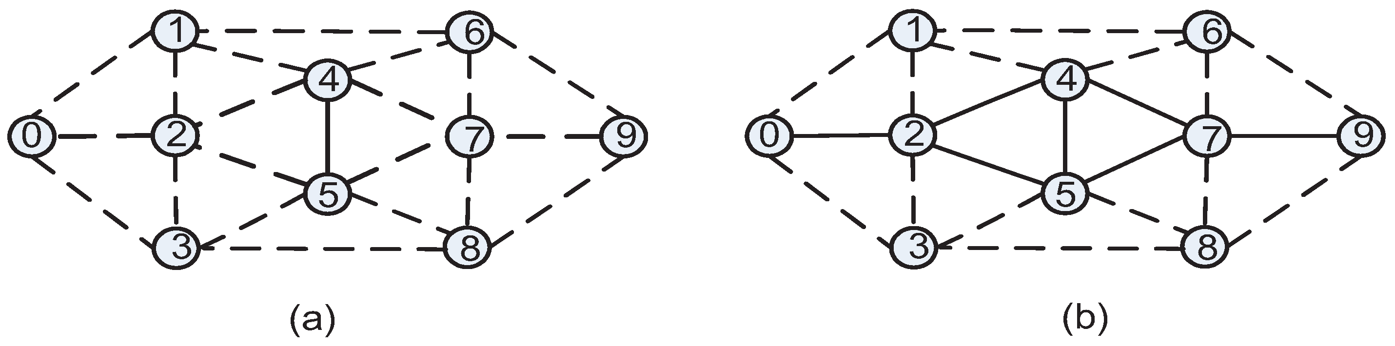
We call this shortest distance between two subgraphs the vertical distance, and the path between two subgraphs with this vertical distance the vertical path. Note that and can be a single node in graph G. For example, in Figure 2a, graph G consists of 10 nodes and 21 links. Denote as , and the part with solid lines in Figure 2b as . Assuming that each edge has the same weight, and equals to 1, the distances between and the nodes in are , , , and ; then the vertical paths between and are , and .
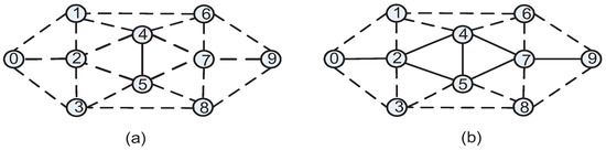
Figure 2.
Vertical distance example. (a) Graph G. (b) The part with solid lines: .
The capacity constraint is considered first before calculating the path for the demand. For all the links in G, if the load of this link will exceed its capacity after taking the current demand bandwidth, then remove it from G temporarily, and the new physical topology is denoted as . If this link belongs to too, remove it from at the same time and denote the new virtual topology as . After this action, all links in the new topology and will meet the bandwidth demand. So the paths calculated based on and can always satisfy the capacity constrain.
To decrease the complexity of CWGA, the communication demands are classified into four cases based on the source node and destination node : (1) and both belong to the virtual topology; (2) belongs to the virtual topology, and not; (3) doesn’t belong to the virtual topology, and does; (4) Neither nor belongs to the virtual topology. The four cases will be treated differently; after calculating the path for , and will be updated according to this path. In the following text, the four cases will be described, each in turn.
CASE (1): and both belong to the virtual topology
As described in Algorithm 1, in this case, first we calculate whether there is a feasible path in (Line 2). To do this, the classical shortest path algorithm (Dijkstra algorithm) is used in function . If there is a path, then a path without changing virtual topology is acquired. Obviously, this is the optimal path for saving energy. If there is not a path, then find the connected nodes of in by calling function (Line 4). Similarly, the Dijkstra algorithm is used in function to get the distances from to the other nodes in . is connected to another node if the distance between them is limited, otherwise they are unconnected. Note that the connected nodes include itself. Then the connected nodes and the links among them in construct a connected sub-topology including of . Similarly, another connected sub-topology including can be revealed by finding the connected nodes of (Line 5). Now we have gotten two connected sub-topologies of . One includes , and the other includes . Since there is no path between and in , the two sub-topologies are not connected. According to the vertical path defined at the beginning of this section, the vertical path of two sub-topologies in can be found (Line 6). Note that, in order to find the least energy consumption path, the energy consumption is used as the weight of link instead of distance in function . Through , the two sub-topologies can be connected. Denote as , so the path from to consists of three parts: to , to , and to . The path from to denoted as can be calculated by calling the function (Line 7), likewise the path from to denoted as (Line 8). In the three parts of the , only the middle part represents additional energy consumption.
Looking at the time complexity of Algorithm 1, the complexity of the Dijkstra algorithm is known as [19]; then the complexity of function is equal to the Dijkstra’s. The maximum complexity of function and DistanceTopology are and , respectively. Thus, the complexity of Algorithm 1 is .
The functions , and are used for the same objective in the other cases; they are omitted to eliminate repetition in the following.
| Algorithm 1 GreenRoutingBoth |
| Input: , , , |
| Output: ; |
|
CASE (2): belongs to the virtual topology, and not
As described in Algorithm 2, in this case, we find the connected set of in first (Line 2), then calculate the vertical path in the next step (Line 3). Denote as . The path from to denoted as in can be calculated by (Line 4). Then the path from to can be acquired through two parts: to , and to .
In Algorithm 2, the complexity of in line 3 is . Then the complexity of Algorithm 2 is .
| Algorithm 2 GreenRoutingOneVs |
| Input: , , , |
| Output: ; |
|
CASE (3): doesn’t belong to the virtual topology, and does
This case is similar to the case 2. The difference is that the vertical paths are from to the connected set of . The algorithm is named as . The complexity of this algorithm is the same as Algorithm 2.
CASE (4): Neither nor belongs to the virtual topology
The processing of this case is described in Algorithm 3. In such a situation, may be empty. If it is, calculate a path in directly by calling function (Line 3). Then end the algorithm. Note that in function , the Dijkstra algorithm is used similarly, but the link weights are set to be the energy consumptions of the links. If it is not, finding the optimal path begins with . Firstly, the vertical path between and is calculated (Line 6). Denote as , then calculate the connected set of in (Line 7). and construct a connected sub-topology which includes (Line 8). Now the case is as same as the case 2, so call the Algorithm 2 in the next step (Line 9); and the optimal path will be obtained. Doing the same procedure begins with , which means calculating vertical paths between and first, then doing the series of steps gets the optimal path (Lines 10∼13). The topology consisting of the sleepy links is denoted as (Line 14). The least energy consumption path from to in denoted as is calculated in the next step (Line 15). Comparing the three paths acquired above, get one with the least additional energy consumption to . If their energy consumptions are the same, then choose the shortest one. If the distance of the paths are the same, choose one randomly (Line 16).
In this case, the complexity of function is equal to Dijkstra’s, and the complexity of other functions is . Thus the complexity of Algorithm 3 is .
| Algorithm 3 GreenRoutingNone |
| Input: , , , |
| Output: ; |
|
Based on the complexity analysis of the four cases, the complexity of CWGA is decreased in three cases. The improved algorithm is called as ICWGA.
6. Performance Analysis
In this section, the performance of ICWGA will be further evaluated by a series of simulations.
6.1. Experimental Scenarios
Two different topology sets are used in the evaluation. One is provided by SND-lib [20]. We choose six topologies with different scales and link densities (Link density refers to the average degree of all nodes) as presented in Table 1. The other one is a set of random topologies generated by Brite [21]. In this set, in order to evaluate the effect of link density on the performance of ICWGA, we generate topologies with the same scale but different link densities. Other parameters of the random topologies refer to reference [22]. For simplicity, we assume that all the capacities of links in two topology sets are set to be 100, and the capacities of nodes are large enough to not cause restriction to the traffic.

Table 1.
The SND-lib topologies sizes.
A dynamic demand matrix is used in the simulations. The number of new flows arriving during each detection period follows a Poisson distribution, and the communication pairs are chosen from all the possible pairs uniformly. The flow size of each demand is set to obey a lognormal distribution which has been proved to close to real traffic in [23]. The duration of each demand is set to follow the exponential distribution based on queuing theory.
6.2. Performance Metrics
Three parameters are used in the evaluation of ICWGA performance:
- : the percentage of links that be turned into sleep mode. For simplicity, we assume that the energy consumption of each link in the network is the same. Thus, the percentage of links that are in sleep mode can represent the energy saving ratio.
- : the average bandwidth utilization of all the active links. Since the aim of the green methods is to use the fewest links to route the traffic, the bandwidth utilization of the active links will be improved. Average bandwidth utilization can be calculated by:where denotes the number of links in the virtual topology.
- and : the increased delay of the paths. For energy saving, some traffic will not be routed in the shortest paths. The delay of these paths will be increased. The impact on delay of ICWGA is observed from two aspects, the increased ratio of propagation delay denoted as , and the increased number of hops of a path denoted as . The number of hops is used to evaluate the other delays caused by the switches.
6.3. Results
In this subsection, the results of the simulations are presented. The simulations are conducted to test the behavior of the network as the average arrival ratio of the traffic demand changes.
6.3.1. The Performance Profile of ICWGA
First, through the results for SND-Lib topologies, we observe the performance profile of ICWGA. Since the trend of results for the six topologies are similar, the results for three topologies are presented, and the results for the other three topologies are omitted.
- (1).
- The improvement in energy saving ratio
In order to observe the performance in energy saving of ICWGA, we compare it with the solution of the MILP model which is solved using the IBM ILOG CPLEX Optimizer [24], and a simple uncoordinated sleeping scheme, in which the traffic is routed on the shortest path by using the Dijkstra routing algorithm and the idle links are put into sleep (dubbed simply as Dijkstra in the results). The initial status of the network is generated in a random way.
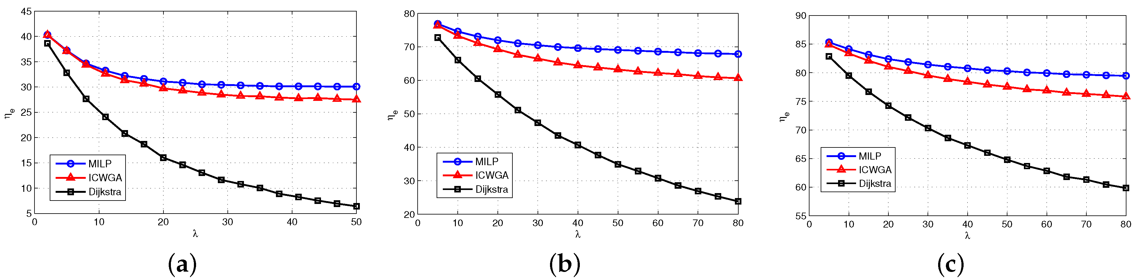
Figure 3 shows the results for energy saving ratio of the different SND-lib topologies. It is observed that, for all the topologies, as increases the energy saving ratio decreases in all the three methods. The two green methods perform much better than the Dijkstra algorithm in energy saving. When , compared with the Dijkstra algorithm, ICWGA achieves about 20% improvement in energy saving for the Abilene topology. Regarding the two relatively large topologies, compared with the Dijkstra algorithm, when ICWGA gets about 36% improvement in energy saving for the India topology, and 16% for the Germany topologies. In all the cases, these improvements are close to optimal solution achieved by solving the MILP model.
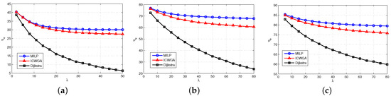
Figure 3.
The results for energy saving ratio of SND-Lib topologies. (a) Abilene. (b) India. (c) Germany.
- (2).
- The improvement in the average bandwidth utilization
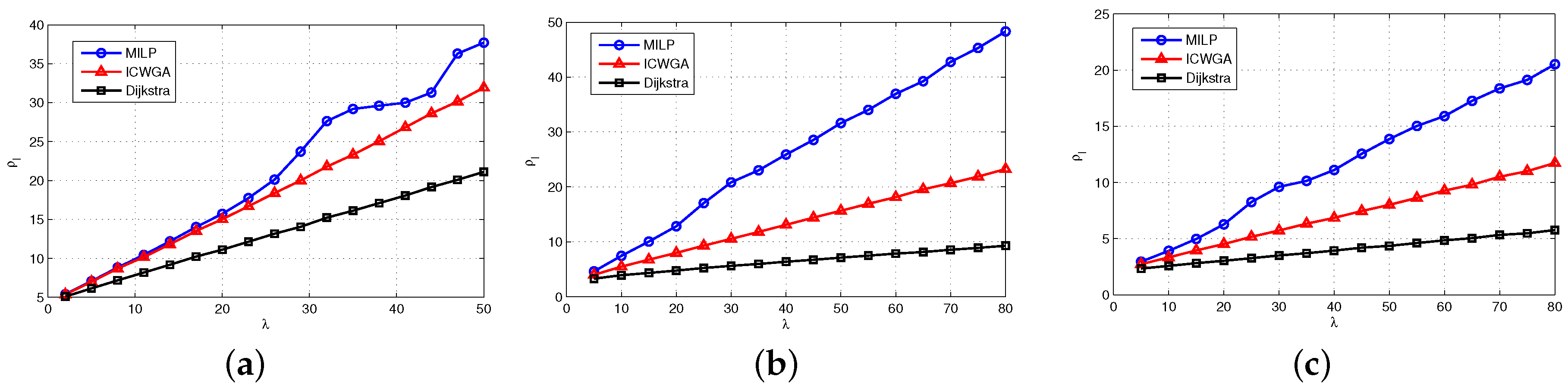
The results for average bandwidth utilization of ICWGA are also compared with those of the MILP model and the Dijkstra algorithm. Figure 4 shows the results for average bandwidth utilization of the three methods. Coinciding with the energy saving results reported in Figure 3, the average bandwidth utilizations of the two green methods are higher than those of the Dijkstra algorithm. In each topology, for the same , the more the energy saving the network realizes, the higher the average bandwidth utilization of the network is. For example, for the India topology, in the case, the energy saving ratio is 14% achieved by the Dijkstra algorithm, 61% by ICWGA, and 69% by the MILP model. The corresponding average bandwidth utilization of the links are 10%, 24%, and 49% respectively.
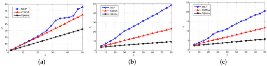
Figure 4.
The results for average bandwidth utilization of different SND-Lib topologies. (a) Abilene. (b) India. (c) Germany.
- (3).
- The effect on the delay caused by ICWGA
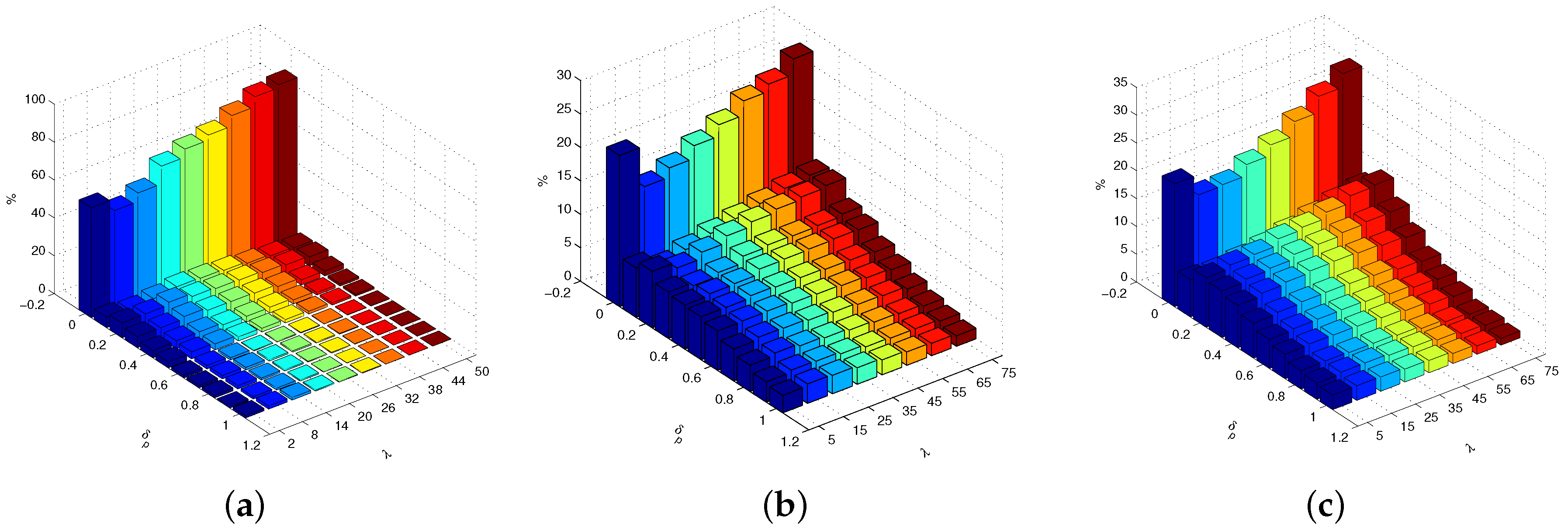
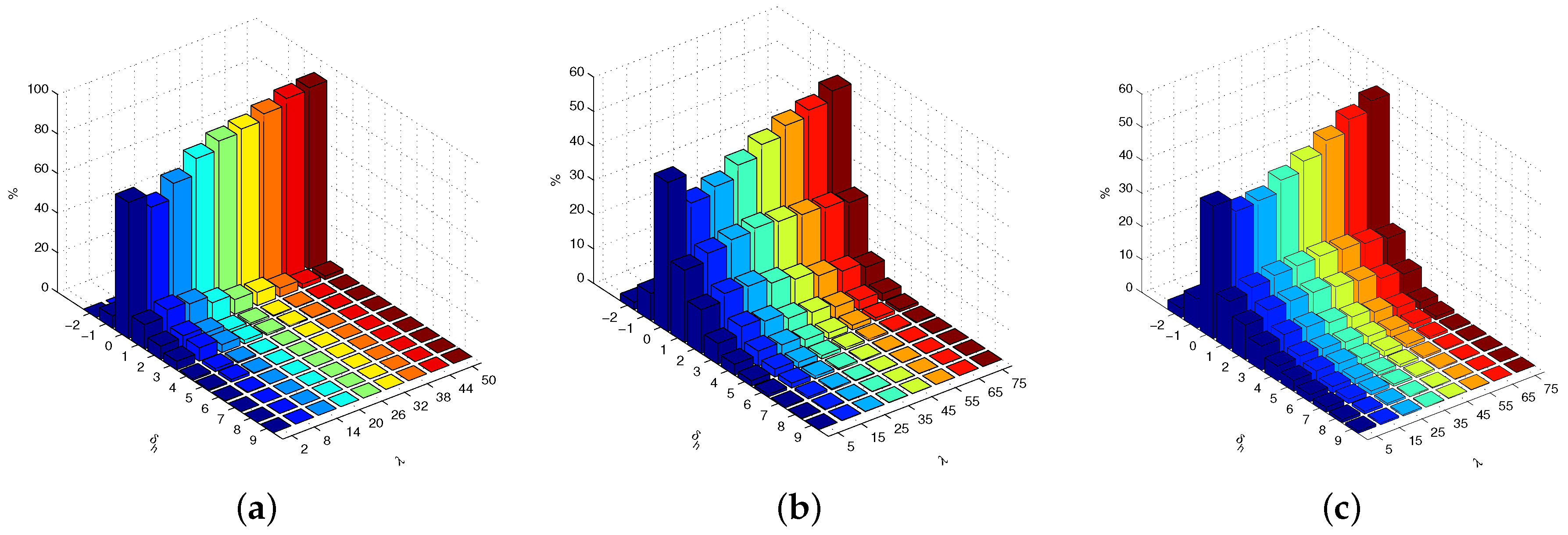
To acquire a more accurate statistical result for the increased delay of the paths, tests are done with 100 (times) * 100 (periods). The increased propagation delay and the increased number of the hops of all the paths are recorded and the distribution results are presented. Figure 5 and Figure 6 show the tradeoff between energy saving and delay caused by ICWGA of the three topologies. For a more clear presentation, for each topology, only the results for half of the cases are shown. It can be seen that in each case, either for the propagation delay or for the improved number of hops, the percentage of 0 accounts for the largest part. For all the topologies, as increases the percentage of 0 gradually increases except for the smallest of cases. As shown in Figure 5, for the increased propagation delay, 0 accounts for 85% when in the Abilene topology, 27% when in the India topology, and 30% when in the Germany topology. The other part accounts for a small percentage. For the increased number of hops, as presented in Figure 6, there even exist some regions corresponding to the negative increased hop numbers, which means the paths calculated by ICWGA pass fewer hops than the shortest paths. This is because the shortest paths are calculated based on the propagation delay in the simulation. Compared to the results for the propagation delay, the 0 parts account for bigger percentages, 92% when for the abilene topology, 52% when for the India topology, and 55% when for the Germany topology; the percentage of 1 accounts for the largest part in the other cases.

Figure 5.
The results for the increased propagation delay of different SND-Lib topologies. (a) Abilene. (b) India. (c) Germany.
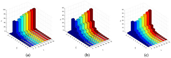
Figure 6.
The results for the increased number of hops of different SND-Lib topologies. (a) Abilene. (b) India. (c) Germany.
In real networks, in order to avoid affecting user experience, we can set a higher priority for the delay sensitive services and route them on the shortest paths, or employ other methods.
6.3.2. The Effect of Some Factors on the Performance of ICWGA
- (1).
- The effect on the performance of ICWGA caused by link density
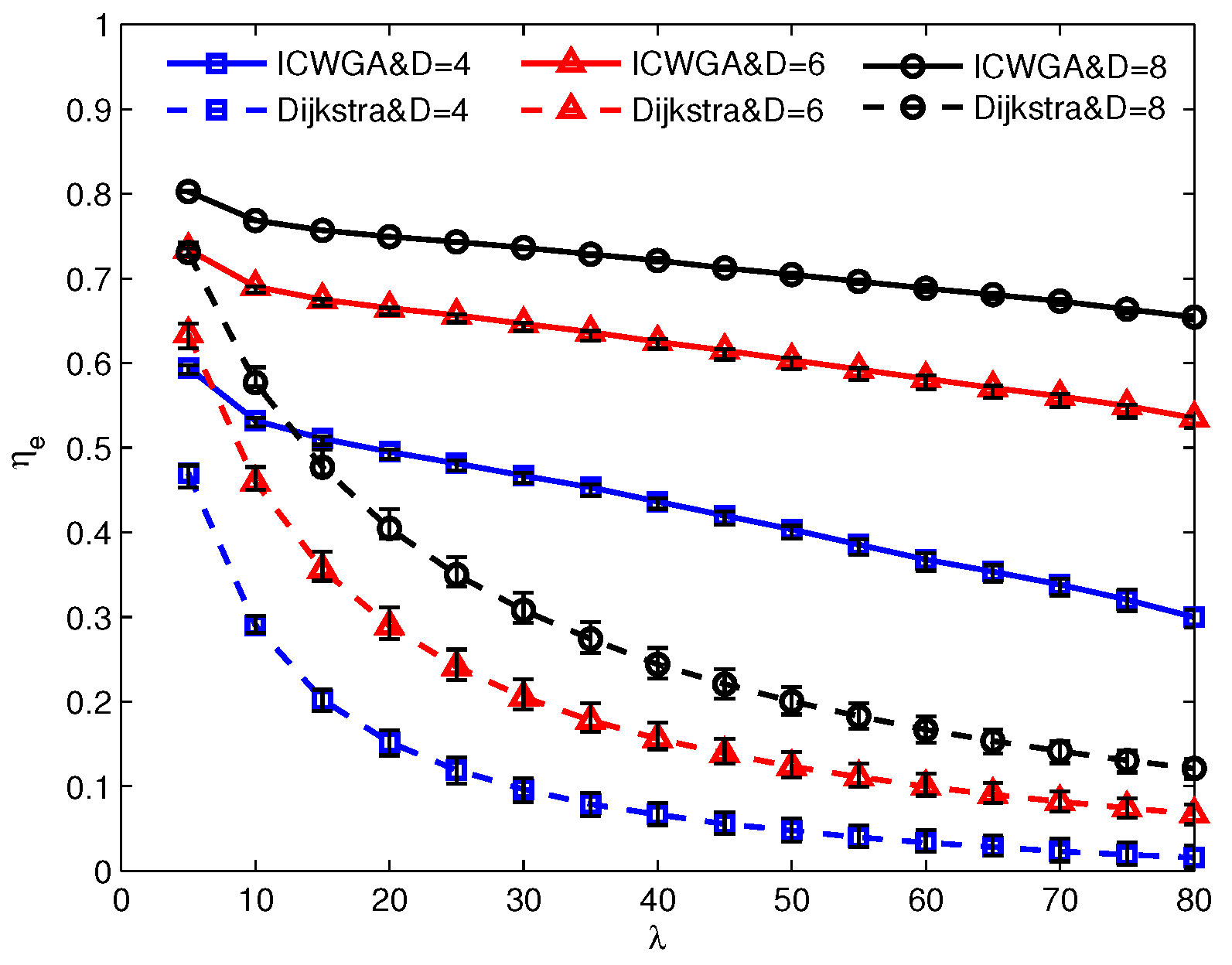
In order to evaluate the effect of link density on ICWGA, three sets of random topologies with same number of nodes and different link densities generated by Brite are used. Each set includes five random topologies. Link density is denoted as D in the results. In the simulation, the number of the nodes , and .
Figure 7 shows the energy saving ratio for the random topology sets. The curves present the averages of the results for the five topologies with the same link density. The error bars show the maximum and minimum values of the results for same cases in a same topology set. It is observed that the difference among the results for the five topologies in a same topology set presented by the height of the error bars are very small and can be ignored. The trend of curves is similar to that of the results for the SND-lib topologies. As increases, the energy saving ratio decreases in all cases, and the decrease rate of ICWGA is slower than that of Dijkstra. Comparing the results for the three topology sets with different link densities, the energy saving ratio increases as the link density increases, and the topology set with achieves the highest energy saving ratio.
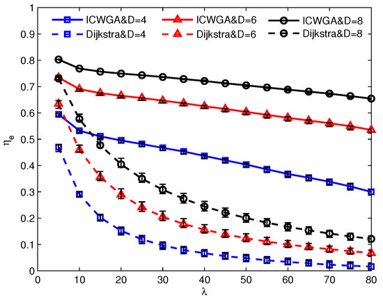
Figure 7.
Energy saving of different link densities.
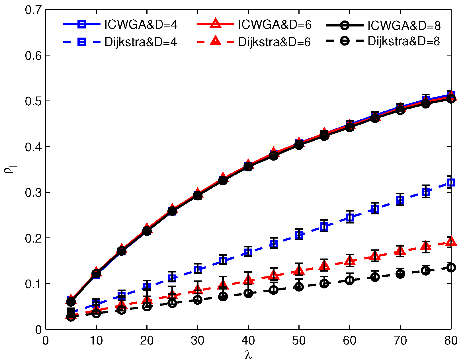
Looking at the average bandwidth utilization of each case in Figure 8, similar to the results in Figure 7, the differences among the results for the five topologies in a same topology set can also be ignored. It is observed that the curves of ICWGA almost overlap. That is to say, no matter how rich the connection of the network is, the number of used links in ICWGA are almost the same under the same traffic load. But for Dijkstra algorithm, the average bandwidth utilization decreases with increasing link density.
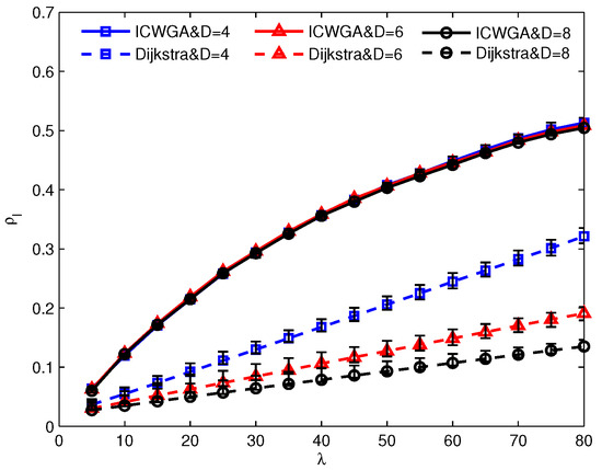
Figure 8.
Average bandwidth utilization of different link densities.
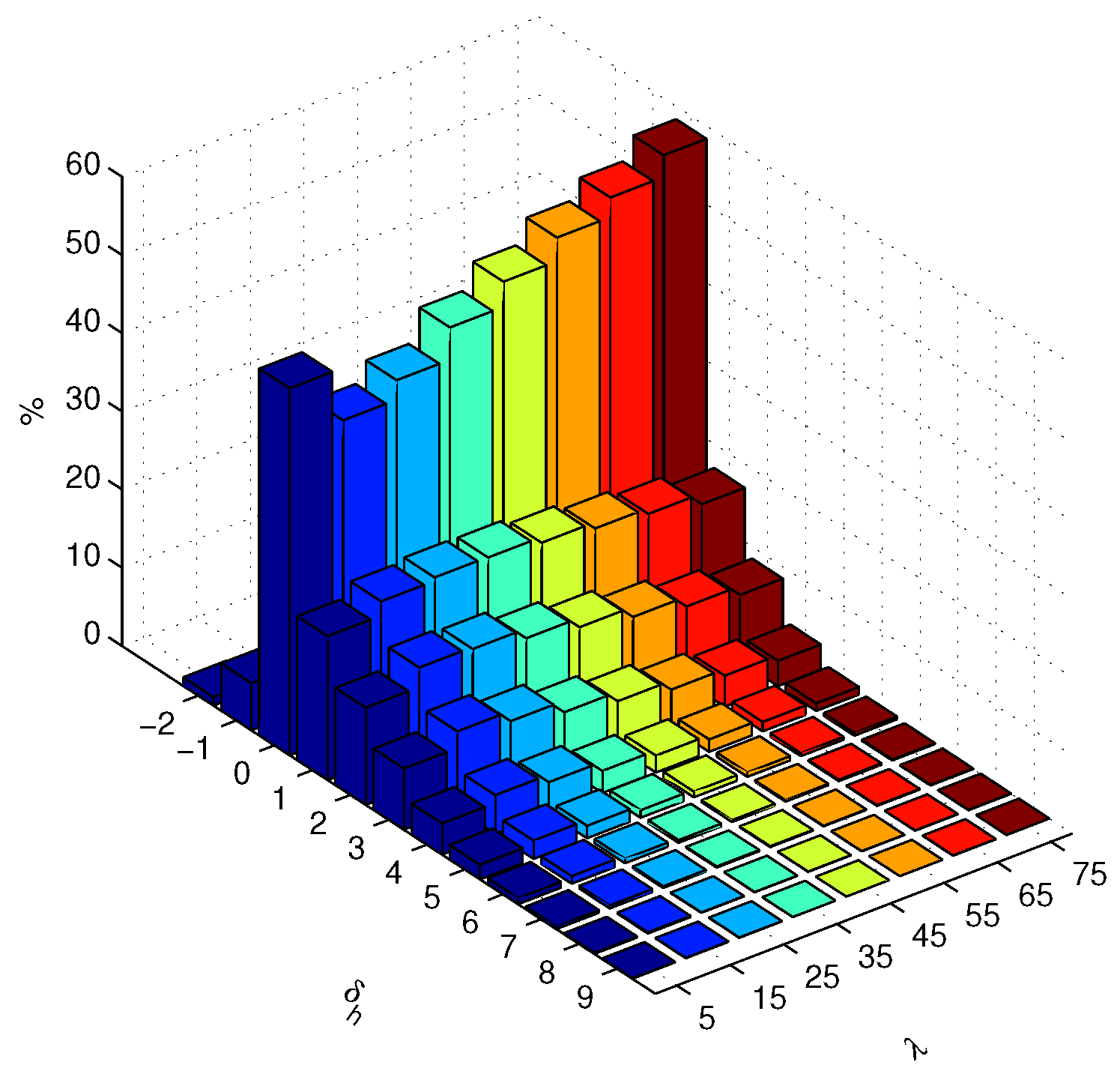
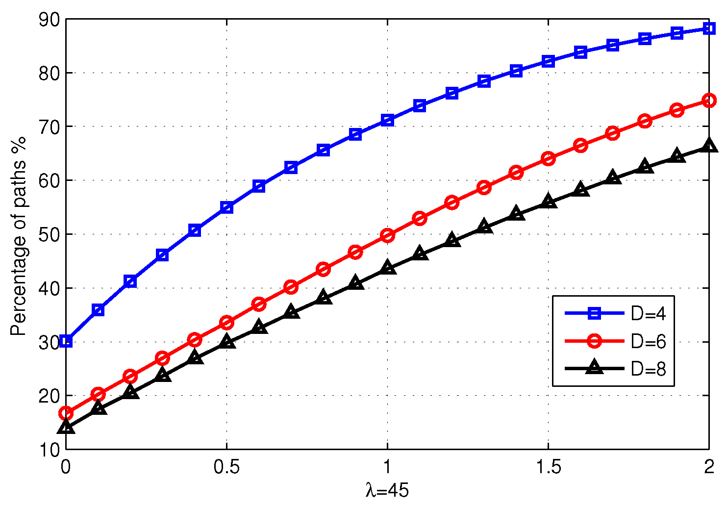
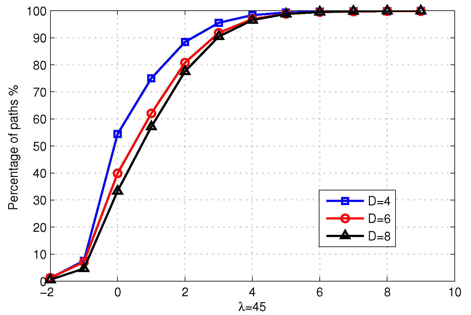
Figure 9 and Figure 10 show the effect on delay caused by ICWGA in the topology set with . The height of the bars show the averages of the results for the five topologies with . They show similar trends to the results for the SND-lib topoligies. Since the trend of results for the other topology sets are similar to those for the topology set with , they are omitted. To compare the effect on the delay caused by link density, the cumulative distribution of the increased delay and the increased number of hops is further examined. Since the trend of all the cases are similar, only the results of the middle one are presented. As shown in Figure 11 and Figure 12, the results for the topology set with perform best in all the cases. The second is the topology set with , and the results for the topology set with is last. It is observed that the richer the network connection is, the worse the effect on the delay the ICWGA causes.
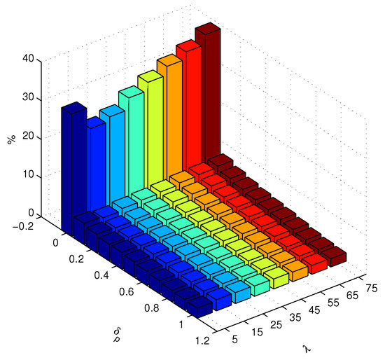
Figure 9.
The distribution of the increased propagation delay for the topology set with .

Figure 10.
The distribution of the increased number of hops for the topology set with .
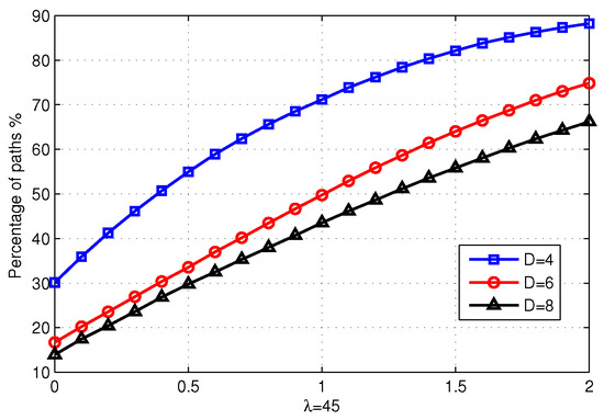
Figure 11.
The cumulative distribution of the increased propagation delay for the topologies with .
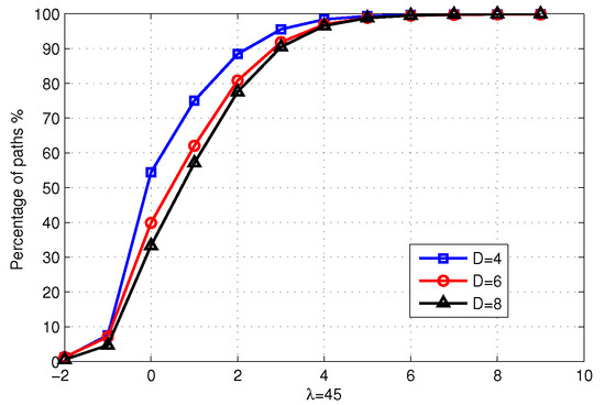
Figure 12.
The cumulative distribution of the increased number of hops for the topologies with .
Based on the analysis above, it can be concluded that, under the same traffic load, the richer the connection of the network is, the higher the energy saving ratio ICWGA achieves, but the impact on the delay will be larger.
- (2).
- The effect of processing sequence on performance of ICWGA
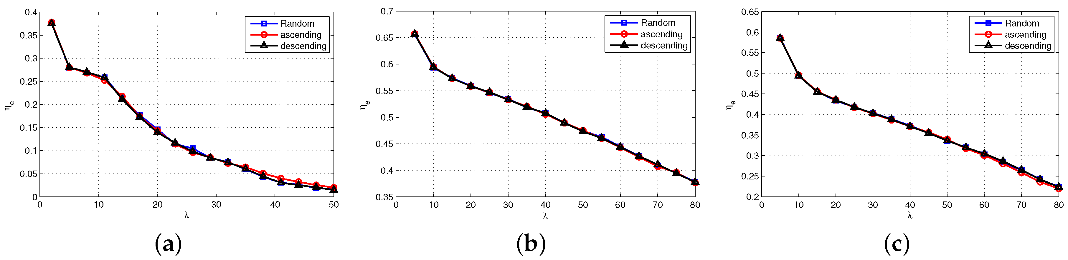
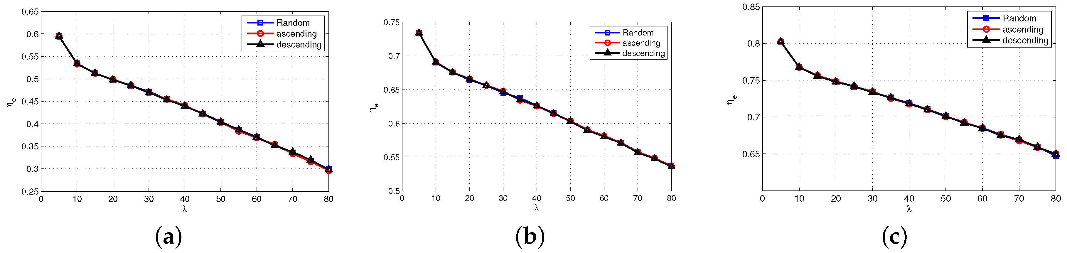
When traffic demands arrive at the same time, the processing order may affect the performance of ICWGA. According to the demand bandwidth of traffic, three orders are considered, random, ascending, and descending. Six topologies are used in the evaluation, three from SND-lib and three random topologies.
Figure 13 and Figure 14 show the effect on energy saving ratio of the three processing orders. Obviously, for every topology, the curves of three different orders almost overlap, which means the differences among the three processing orders are little under this network scale. Figure 13 shows that for different scale of network, the performance in energy saving of the three orders is almost the same. The results presented in Figure 14 show that for different link densities the effect of orders is the same.
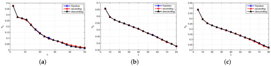
Figure 13.
Different processing sequence in SND-lib topologies. (a) Abilene. (b) India. (c) Germany.
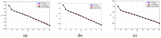
Figure 14.
Different processing sequence in random topologies. (a) . (b) . (c) .
For the results of average bandwidth utilization and the increased delay, three orders present almost the same results as in the aspect of energy saving ratio, so they are omitted.
7. Conclusions
As a new network architecture, SDN is attracting widespread attention in the field because of its high controllability and flexibility. With SDN developing and deploying gradually, it is advisable that we make full use of its controllability to consider the green problem, and it will improve the energy efficiency of the network greatly. In this paper, to improve the energy efficiency a green scheme based on the virtual topology in the SDN architecture was designed, in which paths are chosen based on the working status of the network, and detecting the link status periodically. To achieve the optimal solution of energy saving, the problem was formulated as a MILP model. Owing to the high complexity of the model, an improved heuristic routing algorithm named ICWGA was further studied to achieve better performance. Through a series of simulations, the performance of ICWGA was further examined. The results showed that ICWGA performs well in energy saving, achieving 16∼36% improvement in energy saving compared with the Dijkstra algorithm in the test cases.
Acknowledgments
This work is supported in part by Program for National Natural Science Foundation of China under Grant No. 61571065.
Author Contributions
Ying Hu and Tao Luo initiated and discussed the research problem; Ying Hu and Norman C. Beaulieu developed the model of the problem; Ying Hu and Wenjie Wang performed the simulation and analyzed the data; Ying Hu and Norman C. Beaulieu prepared and wrote the paper.
Conflicts of Interest
The authors declare no conflict of interest.
References
- McKeown, N.; Anderson, T.; Balakrishnan, H.; Parulkar, G.; Peterson, L.; Rexford, J.; Shenker, S.; Turner, J. OpenFlow: Enabling innovation in campus networks. ACM SIGCOMM Comput. Commun. Rev. 2008, 38, 69–74. [Google Scholar] [CrossRef]
- Pickavet, M.; Vereecken, W.; Demeyer, S.; Audenaert, P.; Vermeulen, B.; Develder, C.; Colle, D.; Dhoedt, B.; Demeester, P. Worldwide energy needs for ICT: The rise of power-aware networking. In Proceedings of the 2008 2nd International Symposium on Advanced Networks and Telecommunication Systems, Mumbai, India, 15–17 December 2008; pp. 1–3. [Google Scholar]
- Jain, S.; Kumar, A.; Mandal, S.; Ong, J.; Poutievski, L.; Singh, A.; Venkata, S.; Wanderer, J.; Zhou, J.; Zhu, M. B4: Experience with a globally-deployed software defined wan. In Proceedings of the ACM SIGCOMM 2013 Conference on SIGCOMM, Hong Kong, China, 12–16 August 2013; pp. 3–14. [Google Scholar]
- Chabarek, J.; Sommers, J.; Barford, P.; Estan, C.; Tsiang, D.; Wright, S. Power awareness in network design and routing. In Proceedings of the 27th IEEE Conference on Computer Communications (INFOCOM 2008), Phoenix, AZ, USA, 13–18 April 2008. [Google Scholar]
- Bousia, A.; Antonopoulos, A.; Alonso, L.; Verikoukis, C. “Green” distance-aware base station sleeping algorithm in LTE-Advanced. In Proceedings of the IEEE International Conference on Communications, Ottawa, ON, Canada, 10–15 June 2012; pp. 1347–1351. [Google Scholar]
- Bousia, A.; Kartsakli, E.; Alonso, L.; Verikoukis, C. Dynamic energy efficient distance-aware Base Station switch on/off scheme for LTE-advanced. In Proceedings of the 2012 IEEE Global Communications Conference (GLOBECOM), Anaheim, CA, USA, 3–7 December 2012; pp. 1532–1537. [Google Scholar]
- Oh, E.; Son, K.; Krishnamachari, B. Dynamic Base Station Switching-on/off Strategies for Green Cellular Networks. IEEE Trans. Wirel. Commun. 2013, 12, 2126–2136. [Google Scholar] [CrossRef]
- Niu, Z.; Wu, Y.; Gong, J.; Yang, Z. Cell zooming for cost-efficient green cellular networks. IEEE Commun. Mag. 2010, 48, 74–79. [Google Scholar] [CrossRef]
- Bousia, A.; Kartsakli, E.; Antonopoulos, A.; Alonso, L.; Verikoukis, C. Multiobjective Auction-Based Switching-off Scheme in Heterogeneous Networks: To Bid or Not to Bid? IEEE Trans. Veh. Technol. 2016, 65, 9168–9180. [Google Scholar] [CrossRef]
- Gupta, M.; Singh, S. Greening of the Internet. In Proceedings of the 2003 Conference on Applications, Technologies, Architectures, and Protocols for Computer Communications, ACM, Karlsruhe, Germany, 25–29 August 2003; pp. 19–26. [Google Scholar]
- Addis, B.; Capone, A.; Carello, G.; Gianoli, L.G.; Sanso, B. Energy management through optimized routing and device powering for greener communication networks. IEEE/ACM Trans. Netw. (TON) 2014, 22, 313–325. [Google Scholar] [CrossRef]
- Shen, G.; Tucker, R. Energy-minimized design for IP over WDM networks. IEEE/OSA J. Opt. Commun. Netw. 2009, 1, 176–186. [Google Scholar] [CrossRef]
- Heller, B.; Seetharaman, S.; Mahadevan, P.; Yiakoumis, Y.; Sharma, P.; Banerjee, S.; McKeown, N. ElasticTree: Saving Energy in Data Center Networks. NSDI 2010, 10, 249–264. [Google Scholar]
- Hu, Y.; Luo, T.; Wang, W.; Deng, C. GreSDN: Toward a green software defined network. In Proceedings of the 2016 18th Asia-Pacific Network Operations and Management Symposium (APNOMS), Kanazawa, Japan, 5–7 October 2016; pp. 1–6. [Google Scholar]
- Hu, Y.; Luo, T.; Beaulieu, N.; Deng, C. The Energy-Aware Controller Placement Problem in Software Defined Networks. IEEE Commun. Lett. 2016. [Google Scholar] [CrossRef]
- Ruiz-Rivera, A.; Chin, K.W.; Soh, S. GreCo: An Energy Aware Controller Association Algorithm for Software Defined Networks. IEEE Commun. Lett. 2015, 19, 541–544. [Google Scholar] [CrossRef]
- Tu, R.; Wang, X.; Yang, Y. Energy-saving model for SDN data centers. J. Supercomput. 2014, 70, 1477–1495. [Google Scholar] [CrossRef]
- Giroire, F.; Moulierac, J.; Phan, T.K. Optimizing Rule Placement in Software-Defined Networks for Energy-aware Routing. In Proceedings of the IEEE GLOBECOM, Austin, TX, USA, 8–12 December 2014. [Google Scholar]
- Barbehenn, M. A note on the complexity of Dijkstra’s algorithm for graphs with weighted vertices. IEEE Trans. Comput. 1998, 47, 263. [Google Scholar] [CrossRef]
- SNDlib: Library of Test Instance for Survivable Fixed Telecommunication Network Design. 2006. Available online: http://sndlib.zib.de/home.action (accessed on 15 August 2014).
- Brite: Boston University Representative Internet Topology Generator. Available online: http://www.cs.bu.edu/brite/ (accessed on 21 May 2015).
- Heckmann, O.; Piringer, M.; Schmitt, J.; Steinmetz, R. Generating realistic ISP-level network topologies. IEEE Commun. Lett. 2003, 7, 335–336. [Google Scholar] [CrossRef]
- Nucci, A.; Sridharan, A.; Taft, N. The problem of synthetically generating IP traffic matrices: Initial recommendations. ACM SIGCOMM Comput. Commun. Rev. 2005, 35, 19–32. [Google Scholar] [CrossRef]
- CPLEX: IBM’s Linear Programming Solver. 2014. Available online: http://www.ilog.com/product/cplex/ (accessed on 21 October 2014).

© 2017 by the authors. Licensee MDPI, Basel, Switzerland. This article is an open access article distributed under the terms and conditions of the Creative Commons Attribution (CC BY) license (http://creativecommons.org/licenses/by/4.0/).