Improved Image Denoising Algorithm Based on Superpixel Clustering and Sparse Representation

Abstract

Good learning image priors from the noise-corrupted images or clean natural images are very important in preserving the local edge and texture regions while denoising images. This paper presents a novel image denoising algorithm based on superpixel clustering and sparse representation, named as the superpixel clustering and sparse representation (SC-SR) algorithm. In contrast to most existing methods, the proposed algorithm further learns image nonlocal self-similarity (NSS) prior with mid-level visual cues via superpixel clustering by the sparse subspace clustering method. As the superpixel edges adhered to the image edges and reflected the image structural features, structural and edge priors were considered for a better exploration of the NSS prior. Next, each similar superpixel region was regarded as a searching window to seek the first $L$ most similar patches to each local patch within it. For each similar superpixel region, a specific dictionary was learned to obtain the initial sparse coefficient of each patch. Moreover, to promote the effectiveness of the sparse coefficient for each patch, a weighted sparse coding model was constructed under a constraint of weighted average sparse coefficient of the first $L$ most similar patches. Experimental results demonstrated that the proposed algorithm achieved very competitive denoising performance, especially in image edges and fine structure preservation in comparison with state-of-the-art denoising algorithms.

1. Introduction

As one of the most fundamental low-level vision problems, image denoising has been widely studied in computer vision, serving as the foundation and precondition for image processing, such as visual saliency detection, image segmentation, image classification, etc. In general, image denoising aims at recovering the clean image from the noise-corrupted image while preserving, as much as possible, the vital image features. During the past few decades, image denoising has drawn much research attention, resulting in a variety of efficient methods. Traditional image denoising methods include the median filter, the Gaussian filter, methods based on the total variation, wavelet threshold methods, etc. However, most of these methods frequently ignore the details of image features that include structure, texture, and edge features. To some extent, the ignorance of image details makes these methods suffer from many defects, comprising of over-smoothing, side effect, artifacts, loss of structure and texture features, ambiguousness of edges, etc.

Motivated by the defects in traditional image denoising methods, significant progress has been made in recent years. As image denoising is typically an ill-posed problem, its solution might not be unique. Based on good learning image priors from noise-corrupted images or clean natural images, numerous methods have been proposed to obtain a better solution to the image denoising problem. In particular, nonlocal self-similarity (NSS) and sparsity are two popular image priors with great potential that lead to state-of-the-art performance. Based on the fact that local image details may appear multiple times across the entire image, NSS prompts a series of excellent algorithms for image denoising. The nonlocal means (NLM) [1] algorithm computed a noise-free pixel as the weighted average of pixels with similar neighborhoods in the fixed-size rectangle searching window, and achieved significant enhancement in denoising performance. Inspired by the success of NLM method, Dabov et al. [2] proposed a remarkable collaborative image denoising scheme, called block-matching and 3D filtering (BM3D). In this scheme, nonlocal similar patches were grouped into a 3D cube and collaborative filtering was conducted in the sparse 3D transform domain. The BM3D algorithm ranks among the best performing methods, yet its implementation is complex. Furthermore, the BM3D algorithm is based on classical fixed orthogonal dictionaries, thus lacking data-adaptability. Building on the principle of sparse and redundant representations [3], another category of methods has been developed, which can learn data-adaptive dictionaries for denoising. The K-SVD algorithm [4] has boosted denoising performance significantly. Mairal et al. [5] proposed the learned simultaneous sparse coding (LSSC) algorithm, which used nonlocal self-similarity (NSS) to improve sparse models with simultaneous sparse coding. In Reference [6], Chatterjee et al. clustered image into $K$ groups to enhance the sparse representation via locally learned dictionaries, which took advantage of geometrical structure feature and the NSS prior in spatial domain. Subsequently, Dong et al. [7] observed that the difference between the representation coefficients of original and degraded images was sparse, and added a restriction to ensure the minimization of the $l_1$ norm for the difference. Thus, this model achieved good results in image denoising. By assuming that the matrix of nonlocal similar patches had a low-rank structure, the low-rank minimization based methods [8,9] also achieved very competitive denoising results. Zhang et al. [10] later proposed a patch group (PG) based NSS prior learning scheme to learn explicit NSS models from natural images for high performance denoising, resulting in high peak signal to noise ratio (PSNR) measurements.

Though NSS in low-level vision cues has been widely utilized to improve image denoising performance in most existing methods, we argue that such utilizations of NSS are not sufficiently effective. These methods learn NSS prior via clustering local size-fixed patches extracted from an image, which may neglect the image edge and structural features to some extent. Moreover, in most existing methods, the NSS prior is usually exploited by searching for nonlocal similar patches to a local patch across a size-fixed square searching window, which always leads to massive workload and ignores the similarities between pairs of patches with large spatial distances. Since most existing methods do not make full use of NSS prior in low-level vision cues, it is necessary to learn the prior in mid-level vision cues for a better exploration of the NSS prior.

With the above considerations, this paper proposes to further learn NSS in mid-level vision cues via superpixel clustering using the sparse subspace clustering method. Since the superpixel edges adhere to the image edges and reflect the image structural features, structural and edge information can be considered for a better exploration of the NSS prior by superpixel clustering. Furthermore, this paper proposes an improved algorithm for image denoising by taking advantage of multiple priors to achieve a better denoising performance, including the NSS prior in the spatial domain and sparse transform domain, sparsity, structure, and edge prior. In the proposed algorithm, we first divided the image into multiple superpixels by the simple linear iteration clustering (SLIC) method and grouped superpixels to generate irregular regions by the sparse subspace clustering method with local features. Regarding these regions as searching windows, we sought the first $L$ most similar patches to each local patch. Next, a data-adaptability dictionary for each region was learned to obtain the initial sparse coefficients of local patches extracted from the images. Finally, to improve the effectiveness of the sparse coefficient for each patch, a weighted sparse coding model was constructed by adding a weighted average sparse coefficient of the first $L$ most similar patches to the sparse representation model. Once final sparse coefficients for all patches were acquired, the noise-free image was obtained. Benefiting from two factors, the proposed algorithm achieves enhanced image denoising performance. First, learning the NSS in mid-level vision cues via superpixel clustering promotes a better exploitation of the NSS prior. Furthermore, regarding similar superpixel regions as a searching window can avoid the ignorance of similarities between pairs of patches with large spatial distances, which also contributes to the better exploitation of the NSS prior. Second, a weighted sparse coding model was established, which reduced the impact of noise on sparse representation and improved the accuracy of sparse coefficient for each patch.

The rest of this paper is organized as follows. In Section 2, the basics of the proposed algorithm are described, including the SLIC algorithm, sparse subspace clustering algorithm and sparse representation algorithm. In Section 3, we introduce the proposed denoising model in detail. Next, experimental results and discussion are presented in Section 4. Finally, we make our conclusions in Section 5.

2. Basics of Superpixel Clustering and Sparse Representation (SC-SR) Algorithm

This paper implements a novel image denoising algorithm based on the NSS prior in mid-level vision cues and weighted sparse coding. Before analyzing the proposed denoising algorithm, it is essential to introduce three basic algorithms which play vital roles in realizing the proposed algorithm.

2.1. Simple Linear Iterative Clustering Algorithm for Segmentation

this paper, a simple linear iterative clustering (SLIC) algorithm was selected to generate compact and nearly uniform superpixels, since it has better performance in running speed, superpixel compactness and contour preservation in comparison with other methods [11]. SLIC generates superpixels by clustering pixels based on their similarity in color and proximity in the image plane [12]. This method seamlessly applies to color as well as grayscale images via replacing color similarity with gray information similarity. In this paper, experiments were conducted on grayscale images.

SLIC is essentially a local k-means clustering method. Given the total number of image pixels $N_p$ and the desired number of superpixels $N_s$, cluster centers are sampled at a regular grid $S= \sqrt{N_p∕N_s}$. To speed up the generation of superpixels, SLIC assigns each pixel $p_i$ to the nearest cluster centers within the local region of the pixel $p_i$ rather than the whole image plane. The size of the local region is $2S\times 2S$ that takes the pixel $p_i$ as the center.

For grayscale images, gray and space information are taken into consideration for describing a pixel as a vector. Instead of using a simple Euclidean norm, the distance measure $D_s$ is defined as follows:

$$D_s=d_g+\frac{m}{S}\times d_{xy},$$

(1)

where $d_g$ is the gray distance, and $d_{xy}$ is the plane distance normalized by the grid interval $S$. A variable $m$ is introduced to control the compactness of a superpixel. The greater the value of $m$, the more spatial is emphasized and the more compact the cluster, and we empirically set $m$ to 10 [12]. The values of $d_g$ and $d_{xy}$ are obtained as follows:

$$d_g=\sqrt{{\left(g_i-g_j\right)}^2},$$

(2)

$$d_{xy}=\sqrt{{\left(x_i-x_j\right)}^2+{\left(y_i-y_j\right)}^2},$$

(3)

where $g_i$ and $g_j$ are the gray values of pixel $i$ and $j$; $x_i$ and $x_j$ are the $x$-coordinate values of pixel $i$ and $j$; and $y_i$ and $y_j$ are the $y$-coordinate values of pixel $i$ and $j$.

Given the desired number of superpixels $N_s$, SLIC begins by sampling $M$ regularly spaced cluster centers, which are denoted by feature vectors ${\left\{{\mathit{C}}_{\mathit{k}}={\left[g_k,x_k,y_k\right]}^T\right\}}_{k=1}^M$. To avoid placing a cluster center at an edge pixel or a noisy pixel, the cluster center is moved to the lowest gradient position in a $3\times 3$ neighborhood. Next, each pixel in the image is associated with the nearest cluster center within the local area of the pixel by adopting k-means clustering method.

The segmentation results of SLIC on some benchmark test images are displayed in Figure 1. As shown, SLIC generates compact and nearly uniform superpixels and achieves a good description of the image edges.

2.2. Sparse Subspace Clustering for Noisy Data

Sparse subspace clustering is an outstanding clustering method based on sparse representation, which is able to handle missing or corrupted data. It is based on the fact that each data point in a union of subspaces can be represented as a linear or affine combination of other points. Points are determined to lie in the same subspace by searching for the sparsest combination, which leads to a sparse similarity matrix [13]. Based on the similarity matrix, spectral clustering is adopted to obtain the final clustering result.

Given a data matrix $\mathit{M}=\left[{\mathit{m}}_{\mathbf{1}},{\mathit{m}}_{\mathbf{2}},\dots ,{\mathit{m}}_{\mathit{n}}\right]$, the sparse representation of each point ${\mathit{m}}_{\mathit{i}}\in R^d$ can be obtained by the following optimal problem:

$$min||{\mathit{\partial }}_{\mathit{i}}||{}_1\mathrm{subject} \mathrm{to} {\mathit{m}}_{\mathit{i}}=\mathit{M}{\mathit{\partial }}_{\mathit{i}}$$

(4)

Matrix ${\mathit{M}}_{\widehat{\mathit{i}}}\in R^{d\times \left(n-1\right)}$ is defined as the matrix obtained from $\mathit{M}$ by removing its i-th column, where the subscript $\widehat{i}$ means that there is no $i$. Point ${\mathit{m}}_{\mathit{i}}$ has a sparse representation with respect to the matrix ${\mathit{M}}_{\widehat{\mathit{i}}}$. Next, the optimal problem is equal to the following problem:

$$min||{\mathit{c}}_{\mathit{i}}||{}_1\mathrm{subject} \mathrm{to} {\mathit{m}}_{\mathit{i}}={\mathit{M}}_{\widehat{\mathit{i}}}{\mathit{c}}_{\mathit{i}} \mathrm{and} {\mathit{c}}_{\mathit{i}}{}^{\mathit{T}}\mathit{{\rm I}}=1,$$

(5)

where $\mathit{{\rm I}}$ is a unit vector. Taking noise into consideration, let $\overline{{\mathit{m}}_{\mathit{i}}}={\mathit{m}}_{\mathit{i}}+{\mathit{\eta }}_{\mathit{i}}$. be the i-th corrupted data point, where $||{\mathit{\eta }}_{\mathit{i}}||{}_2\le \epsilon$ and $\epsilon$ are the noise variance. The optimal problem turns to:

$$min||{\mathit{c}}_{\mathit{i}}||{}_1\mathrm{subject} \mathrm{to}||\overline{{\mathit{m}}_{\mathit{i}}}-{\mathit{M}}_{\widehat{\mathit{i}}}{\mathit{c}}_{\mathit{i}}||{}_2\le \epsilon \mathrm{and} {\mathit{c}}_{\mathit{i}}{}^{\mathit{T}}\mathit{{\rm I}}=1$$

(6)

Lasso optimization method [14] is used for recovering the optimal sparse solution from the above equation. With the sparsest representation of each point, a coefficient matrix $\mathit{C}$ ($\mathit{C}=\left[{\mathit{c}}_{\mathbf{1} },{\mathit{c}}_{\mathbf{2}},\dots ,{\mathit{c}}_{\mathit{n}}\right]$ ) can be obtained, which describes the connections between points. Taking the matrix $C$ to establish a directed graph $G=\left(V,E\right)$, the vertices of the graph $V$ are the $n$ data points and the adjacency matrix is the coefficient matrix $\mathit{C}$. Moreover, to make $G$ balanced, a new adjacency matrix $\tilde{C}$ ($\widetilde{C_{ij}}=\left|C_{ij}\right|+\left|C_{ji}\right|$) is built. Subsequently, the Laplacian matrix $L$ is formed by $\mathit{L}=\mathit{D}\mathit{a}-\tilde{\mathit{C}}$, where $\mathit{D}\mathit{a}\in R^{N\times N}$ is a diagonal matrix and meets the condition of $D{a}_{ii}={\displaystyle \sum }_j\widetilde{C_{ij}}$. Finally, spectral clustering method is applied to cluster the eigenvector of the Laplacian matrix to obtain the final cluster result for the whole data points.

In this paper, sparse subspace clustering is adopted to effectively cluster superpixels into regions of similar geometric structure aiming to further learn the NSS prior in mid-level vision cues even in the presence of noise. It is known that better learning of the NSS prior can improve the performance of denoising algorithms based on structure clustering and sparse representation. Instead of clustering size-fixed patches that are inflexibly extracted from images, clustering superpixels takes image edge and structure features into consideration, which leads to a better learning result of the NSS prior.

2.3. Sparse Representation Based Image Denoising

In general, sparse representation works in a patch-based framework, where an image is represented by sparse coefficients of its overlapping patches. Next, the recovery of image is achieved by averaging the sparse representation of all overlapping patches.

Given an image $\mathit{Y}$ with noise, the column vector of $b\times b$ patch at the location of $i$, is denoted as ${\mathit{y}}_{\mathit{i}}={\mathit{R}}_{\mathit{i}}\mathit{Y}$, where $R_i$ is a binary matrix aiming to extract an overlapping patch and convert it to a column vector. The sparse coefficient $\widehat{{\mathit{\alpha }}_{\mathit{i}}}$ of a patch is realized by the optimal solution to the following equation:

$$\widehat{{\mathit{\alpha }}_{\mathit{i}}}=\underset{{\alpha }_i}{argmin}\frac{1}{2}||{\mathit{y}}_{\mathit{i}}-\mathit{D}{\mathit{\alpha }}_{\mathit{i}}||{}_2^2+\zeta ||{\mathit{\alpha }}_{\mathit{i}}||{}_p,$$

(7)

where $p=0,1$, $\mathit{D}$ is known as dictionary, and $\zeta$ is a regularization parameter to keep a balance between sparsity and reconstruction error. Once $\widehat{{\mathit{\alpha }}_{\mathit{i}}}$ is found, the denoising result $\widetilde{{\mathit{y}}_{\mathit{i}}}$ of the image patch ${\mathit{y}}_{\mathit{i}}$ can be computed by ${\tilde{\mathit{y}}}_{\mathit{i}}=\mathit{D}{\mathit{\alpha }}_{\mathit{i}}$. A challenging issue in finding the sparse coefficient $\widehat{{\mathit{\alpha }}_{\mathit{i}}}$ is to choose the dictionary. In brief, a dictionary is a matrix, which is usually obtained by a specific transformation or learned from a large set of clean patches or noisy patches. When the dictionary and sparse coefficients are obtained, the denoised image $\tilde{Y}$ can be reconstructed by aggregating all of the sparse representation of patches as follows [9]:

$$\tilde{\mathit{Y}}={\left({\mathit{R}}_{\mathit{i}}^{\mathit{T}}{\mathit{R}}_{\mathit{i}}\right)}^{-1}\left({{\displaystyle \sum }}_i{\mathit{R}}_{\mathit{i}}^{\mathit{T}}\mathit{D}{\mathit{\alpha }}_{\mathit{i}}\right),$$

(8)

Nonetheless, only the local sparse representation model is employed in denoising problem, which may not lead to a preferable enough solution. Herein, this paper combines good image priors from the noise-corrupted image with sparse representation for a better solution to image denoising problem. The NSS prior in the spatial domain was learned by superpixel clustering, which also generated irregular regions consisting of similar superpixels. By regarding these regions as searching windows, similar patches to a local patch within each region were found. The NSS prior in sparse transform domain utilized a constraint that the weighted average of sparse coefficients for the acquired similar patches of each local patch constrains the sparse coefficient of the local patch to an optimal solution. The NSS priors in both the spatial domain and sparse transform domain were added into the sparse representation model to enhance the image denoising performance of our proposed algorithm. Further details of the proposed algorithm are explained in the next section.

3. Proposed SC-SR Algorithm

In this section, the image denoising model based on superpixel clustering and sparse representation is presented. We first utilized the SLIC algorithm to generate $M$ superpixels that include similar pixels. Next, the NSS prior was further exploited by making use of the sparse subspace clustering algorithm with local features to cluster similar superpixels into a group. In the abnormal region of similar superpixels group, we extracted overlapping patches for training dictionary and sought similar patches to each local patch. Finally, a weighted sparse coding was adopted for better sparse representation. The following is a detailed introduction on the proposed algorithm.

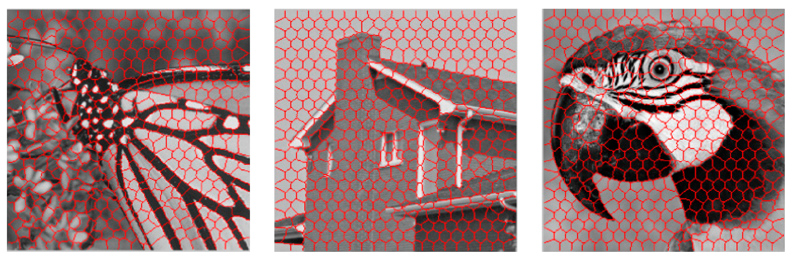
3.1. Superpixels Clustering

the outset, SLIC is used to generate $M$ superpixels, and a superpixel is described as a column vector $u$ with several features. Each image pixel within a superpixel can be represented by a seven-dimensional feature vector $\mathit{f}$:

$$\mathit{f}={\left[g, I_{X }, I_Y, I_{XX}, I_{YY}, \beta \times x, \beta \times y\right]}^T,$$

(9)

where $g$ is the gray value of the pixel; $I_X, I_Y, I_{XX}, I_{YY}$ are the corresponding first or second order derivatives of image intensities in both $X$ and $Y$ axes; and $x$, $y$ are the coordinates of the pixel in an image. The parameter $\beta$ aims to make a balance among image gray, gradient, and spatial features. If we use equal weight ($\beta =1$) for the spatial feature, similarities between pairs of patches with large spatial distances may be lost. Thus, we empirically chose $\beta =0.5$ to alleviate this problem [15]. In addition, the image spatial, gray and gradient values were normalized.

For a given superpixel, we computed the mean vector $u$ of all pixels within it as its feature vector:

$$\mathit{u}=\frac{1}{\Gamma }{{\displaystyle \sum }}_{j=1}^{\Gamma }{\mathit{f}}_{\mathit{j}},$$

(10)

where $\Gamma$ is the size of the superpixel and ${\mathit{f}}_{\mathit{j}}$ indicates a vector of a pixel within the superpixel.

We considered these $N_s$ superpixels as a collection of data points drawn from a union of $K$ independent affine subspaces. The sparse subspace clustering method was adopted to cluster the collection of data points into $K$ groups. After transforming every superpixel into a column vector, the collection of data points $\mathit{U}={\left\{{\mathit{u}}_{\mathit{i}}\right\}}_{i=1}^M$ for clustering was obtained. For each superpixel, its covariance matrix $\mathit{M}\mathit{c}$ was calculated by:

$$\mathit{M}\mathit{c}=\left[\begin{array}{ccc}{\delta }_{11}& \cdots & {\delta }_{17}\\ ⋮& \ddots & ⋮\\ {\delta }_{71}& \cdots & {\delta }_{77}\end{array}\right],$$

(11)

$${\delta }_{ij}=\frac{1}{\Gamma -1}\times \left({{\displaystyle \sum }}_{k=1}^{\Gamma }\left({\mathit{f}}_{\mathit{i}}^{\mathit{k}}-{\mathit{u}}_{\mathit{i}}\right)\times \left({\mathit{f}}_{\mathit{j}}^{\mathit{k}}-{\mathit{u}}_{\mathit{j}}\right)\right),$$

(12)

where ${\mathit{f}}_{\mathit{i}}^{\mathit{k}}$ indicates the i-th feature of the k-th pixel of the current superpixel and ${\mathit{u}}_{\mathit{i}}$ indicates the i-th element of the feature vector of the superpixel.

For two superpixels, their similarity can be computed based on the corresponding covariance matrices, $\mathit{M}{\mathit{c}}_{\mathbf{1}}$ and $\mathit{M}{\mathit{c}}_{\mathbf{2}}$:

$$W\left(\mathit{M}{\mathit{c}}_{\mathbf{1}},\mathit{M}{\mathit{c}}_{\mathbf{2}}\right)=e^{-\rho d\left(\mathit{M}{\mathit{c}}_{\mathbf{1}},\mathit{M}{\mathit{c}}_{\mathbf{2}}\right)},$$

(13)

$$d\left(\mathit{M}{\mathit{c}}_{\mathbf{1}},\mathit{M}{\mathit{c}}_{\mathbf{2}}\right)=\sqrt{{{\displaystyle \sum }}_{i=1}^{7}l{n}^2\left({\lambda }_i\left(\mathit{M}{\mathit{c}}_{\mathbf{1}},\mathit{M}{\mathit{c}}_{\mathbf{2}}\right)\right)},$$

(14)

where $W\mathit{M}({\mathit{c}}_{\mathbf{1}},\mathit{M}{\mathit{c}}_{\mathbf{2}})$ is the similarity of the two superpixels; ${\lambda }_i\left(\mathit{M}{\mathit{c}}_{\mathbf{1}},\mathit{M}{\mathit{c}}_{\mathbf{2}}\right)$ is the generalized eigenvalues from $\left|\lambda \mathit{M}{\mathit{c}}_{\mathbf{1}}-\mathit{M}{\mathit{c}}_{\mathbf{2}}\right|=0$; and $\rho$ is a small constant (we experimentally set $\rho$ to 0.5 in our experiment) [15].

To better characterize the relationship between the superpixels and alleviate the sensitivity of sparse coding to noise, a Laplacian regularization term [15] based on the similarity matrix $W$ was introduced into Equation (6) to ensure the similarity of sparse coefficients among similar superpixels. Next, Equation (6) is equal to the following problem:

$$\begin{gathered} min||\overline{{\mathit{y}}_{\mathit{i}}}-{\mathit{Y}}_{\widehat{\mathit{i}}}{\mathit{c}}_{\mathit{i}}||{}_2+\mu ||{\mathit{c}}_{\mathit{i}}||{}_1+\frac{\gamma }{2}{{\displaystyle \sum }}_{ij}||{\mathit{c}}_{\mathit{i}}-{\mathit{c}}_{\mathit{j}}||{}^2{\mathit{W}}_{\mathit{i}\mathit{j}} \\ = min||\overline{{\mathit{y}}_{\mathit{i}}}-{\mathit{Y}}_{\widehat{\mathit{i}}}{\mathit{c}}_{\mathit{i}}||{}_2+\mu ||{\mathit{c}}_{\mathit{i}}||{}_1+ \gamma tr\left(\mathit{C}\mathit{L}{\mathit{C}}^{\mathit{T}}\right)\mathrm{subject} \mathrm{to}{\mathit{c}}_{\mathit{i}}{}^{\mathit{T}}\mathit{{\rm I}}=1, \end{gathered}$$

(15)

where $\mathit{L}$ is the Laplacian matrix defined as $\mathit{L}={\mathit{D}}_{\mathit{a}}-\mathit{W}$, and ${\mathit{D}}_{\mathit{a}}$ is the diagonal matrix with row sums, ${\mathit{D}}_{\mathit{i}\mathit{i}}={\displaystyle \sum }_j{\mathit{W}}_{\mathit{i}\mathit{j}}$ The parameter $\gamma$ is the weighted parameter that balances the effect of the Laplacian regularization term ($\gamma$ was empirically set to 0.2 in our experiments) [15]. By solving Equation (15), a sparse coefficients matrix $\mathit{C}=\left[\widehat{{\mathit{c}}_{\mathbf{1}}},\widehat{{\mathit{c}}_{\mathbf{2}}},\dots ,\widehat{{\mathit{c}}_{\mathit{M}}}\right]$ was obtained, which was not symmetric. Therefore, we updated it by $C_{ij}=C_{ji}=\left|C_{ij}+C_{ji}\right|$ to make it symmetric. A directed graph $\mathrm{G}=\left(V, E\right)$ was built by utilizing the sparse coefficients matrix $\mathit{C}$. The vertices of the graph $V$ were the data set ${\left\{{\mathit{u}}_{\mathit{i}}\right\}}_{i=1}^M$, and the new adjacent matrix was $\mathit{A}=\mathit{H}-\mathit{C}$, where ${\mathit{H}}_{ii}={\displaystyle \sum }_j{\mathit{C}}_{\mathit{i}\mathit{j}}$ The spectral clustering algorithm was used to segment the graph $G$ to obtain the result of clustering superpixels.

Superpixel clustering learned NSS prior, which contributed to the preservation of structural information of the denoised image. When the dictionary was learned, the learned NSS prior obtained by superpixels clustering added the structural feature and edge feature into the atoms of the dictionary. The richer the features of the dictionary, the stronger the ability to reconstruct original image.

3.2. Learning Sub-Dictionaries for Each Cluster of Superpixels

In the similar superpixel regions, we extracted overlapping patches centering on each pixels, where the overlapping patches were all $b\times b$ size ($b$ is odd). As for the pixels on the boundary of the image, we extended them by $b/2$ pixels in a horizontal and vertical direction by mirroring pixels to gain the patches centering on them. As shown in Figure 2, the matrix $M{a}_1$ was extended by two elements in a horizontal and vertical direction by mirroring extension, and the matrix $M{a}_2$ was obtained. After every patch was transformed into a column vector, $K$ sub-datasets ${\left\{{\mathit{M}}_{\mathit{k}} \right\}}_{k=1}^K$ were formed for training sub-dictionaries.

Since the number of patches in each cluster was limited and patches in ${{\rm M}}_k$ had similar patterns, it was not necessary to learn an over-complete dictionary for each cluster [16]. Therefore, we used the principal component analysis (PCA) method to learn the compact sub-dictionary for each cluster.

For each sub-dataset ${\mathit{M}}_k$, the proposed algorithm applied PCA to compute the principal components, with the purpose of constructing the sub-dictionaries ${\left\{{\mathit{D}}_{\mathit{k}} \right\}}_{k=1}^K$. ${\mathit{D}}_{\mathit{k}}$ can be constructed by the optimal solution for the following formulation:

$$\left(\widehat{{\mathit{D}}_{\mathit{k}}},\widehat{{\mathit{A}}_{\mathit{k}}}\right)=arg\underset{D_k,A_k}{min}\left\{||{\mathit{M}}_{\mathit{k}}-{\mathit{D}}_{\mathit{k}}{\mathit{A}}_{\mathit{k}}||{}_2^2+\lambda ||{\mathit{A}}_{\mathit{k}}||{}_1\right\},$$

(16)

where ${\mathit{A}}_{\mathit{k}}$ is the sparse coefficient matrix of ${\mathit{M}}_{\mathit{k}}$ over ${\mathit{D}}_{\mathit{k}}$ The rank of ${\mathit{M}}_{\mathit{k}}$ is denoted by $r$ and the co-variance matrix of ${\mathit{M}}_{\mathit{k}}$ is denoted by ${\mathit{\psi }}_{\mathit{k}}$ We obtained the result of matrix factorization ${\mathit{\psi }}_{\mathit{k}}={\mathit{P}}_{\mathit{k}}^{\mathit{T}}{\mathit{\Lambda }}_{\mathit{k}}{\mathit{P}}_{\mathit{k}}$, where ${\mathit{P}}_{\mathit{k}}=\left[{\mathit{p}}_{\mathbf{1}},{\mathit{p}}_{\mathbf{2}},\dots ,{\mathit{p}}_{\mathit{r}}\right]$ is the orthogonal transformation matrix and ${\mathit{\Lambda }}_{\mathit{k}}$ is a diagonal matrix taking $r$ eigenvalues of ${\mathit{\psi }}_{\mathit{k}}$ as its diagonal elements. If we regard ${\mathit{P}}_{\mathit{k}}$ as the dictionary and set ${\mathit{E}}_{\mathit{k}}={\mathit{P}}_{\mathit{k}}^{\mathit{T}}{\mathit{M}}_{\mathit{k}}$, we obtain $||{\mathit{{\rm M}}}_{\mathit{k}}-{\mathit{P}}_{\mathit{k}}{\mathit{E}}_{\mathit{k}}||{}_2^2=||{\mathit{{\rm M}}}_{\mathit{k}}-{\mathit{P}}_{\mathit{k}}{\mathit{P}}_{\mathit{k}}^{\mathit{T}}{\mathit{M}}_{\mathit{k}}||{}_2^2=0$ Therefore, Equation (16) is only determined by the sparsity regularization term ${\mathit{E}}_{\mathit{k}}{}_1$, which is constant in this case. To obtain better sub-dictionaries for sparse representation, we extracted the first $\tau \in \left[1,r\right]$ most important eigenvectors in ${\mathit{P}}_{\mathit{k}}$ to form a dictionary ${\mathit{D}}_{\mathit{k}}^{\mathit{\tau }}$, ${\mathit{D}}_{\mathit{k}}^{\mathit{\tau }}=\left[{\mathit{p}}_{\mathbf{1}},{\mathit{p}}_{\mathbf{2}},\dots ,{\mathit{p}}_{\mathit{\tau }}\right]$, instead of regarding ${\mathit{P}}_{\mathit{k}}$ as the dictionary. The sparse coefficient matrix is denoted by ${\mathit{A}}_{\mathit{k}}^{\mathit{\tau }}$ It is known that ${\mathit{E}}_{\mathit{k}}{}_1$ increases when $\tau$ increases, while $||{\mathit{{\rm M}}}_{\mathit{k}}-{\mathit{D}}_{\mathit{k}}^{\mathit{l}}{\mathit{A}}_{\mathit{k}}^{\mathit{l}}||{}_2^2$ decreases. The optimal solution can be obtained by solving the following problem:

$$\widehat{\tau }=\underset{\tau }{argmin}\left\{||{\mathit{{\rm M}}}_{\mathit{k}}-{\mathit{D}}_{\mathit{k}}^{\mathit{\tau }}{\mathit{A}}_{\mathit{k}}^{\mathit{\tau }}||{}_2^2+\lambda ||{\mathit{A}}_{\mathit{k}}^{\mathit{\tau }}||{}_1\right\}.$$

(17)

Consequently, we obtained $K$ sub-dictionaries ${\left\{{\mathit{D}}_{\mathit{k}} \right\}}_{k=1}^K$ for the $K$ sub-datasets ${\left\{{\mathit{M}}_{\mathit{k}} \right\}}_{k=1}^K$ In Equation (17), it was verified that some noise can be successfully removed during computing the local PCA transform of each image patch. In this paper, PCA was applied to each sub-dataset to construct the dictionary, which was able to reduce not only the computational cost consumed by dictionary training, but also the noise introduced into the dictionary.

3.3. Sparse Representation Model for Image Denoising

It was addressed that similar patches shared the same dictionary elements in their sparse decomposition [5]. In other words, there was NSS in the sparse transform domain as well. The proposed algorithm takes advantage of that fact to achieve a better sparse representation and improve the performance of image denoising.

In the previous subsection, we learned a PCA dictionary for each cluster. Given the dictionaries, the initial sparse coefficients ${\mathit{\alpha }}_{\mathit{i}}^{\left(\mathbf{0}\right)}$ of all patches within each cluster are found by solving the minimization problem of Equation (7) in the condition of $p=0$ It is known that ${\ell }_0$ pseudo norm regularization term has usually better reconstruction performance than ${\ell }_1$ pseudo norm regularization term [17]. Since ${\ell }_0$ minimization problem is NP-hard, greedy approaches are employed to achieve an approximate solution. One of the most widely used greedy approach is the orthogonal matching pursuit (OMP) that successively selects the best atom of dictionary minimizing the representation error until a stopping criterion is satisfied. In our algorithm, we employed a modified version of OMP, referred to as generalized OMP (GOMP) [18], to obtain the initial sparse coefficients ${\mathit{\alpha }}_{\mathit{i}}^{\left(\mathbf{0}\right)}$, which allowed the selection of multiple atoms per iteration. Simultaneous selection of multiple atoms reduced the number of iterations and achieved better sparse representation.

After obtaining the initial sparse coefficients ${\mathit{\alpha }}_{\mathit{i}}^{\left(\mathbf{0}\right)}$, we exploited the NSS prior in the sparse transform domain to produce a better estimate of the original image. To begin, we looked for the first $L$ most similar patches to each patch across the region of similar superpixels. Each pixel in a patch was denoted as a column vector that is computed by Equation (9), and the patch with the size of $b\times b$ was described as a matrix ${\mathit{P}}_{\mathit{i}}=\left[{\mathit{f}}_{{\mathit{i}}_{\mathbf{1}}},{\mathit{f}}_{{\mathit{i}}_{\mathbf{2}}},\dots ,{\mathit{f}}_{{\mathit{i}}_{{\mathit{b}}^{\mathbf{2}}}}\right]$ The similarity between the two patches was measured by Equation (13) with their covariance matrixes. After obtaining the patches similar to each local patch, we computed the weighted average of initial sparse coefficients associated with the similar patches as ${\mathit{\chi }}_{\mathit{i}}$ Next, ${\mathit{\chi }}_{\mathit{i}}$ was exploited to constrain the sparse coefficient of the local patch to reduce the impact of noise on sparse representation and achieve a better solution. A better sparse representation coefficient for each patch ${\mathit{y}}_{\mathit{i}}$ can be found by:

$$\widehat{{\mathit{\alpha }}_{\mathit{i}}}=\underset{{\mathit{\alpha }}_{\mathit{i}}}{argmin}||{\mathit{y}}_{\mathit{i}}-\mathit{D}{\mathit{\alpha }}_{\mathit{i}}||{}_2^2+\eta ||{\mathit{\alpha }}_{\mathit{i}}-{\mathit{\chi }}_{\mathit{i}}||{}_1,$$

(18)

$${\mathit{\chi }}_{\mathit{i}}={{\displaystyle \sum }}_{j=1}^L{w}_{ij}{\mathit{\alpha }}_{\mathit{j}}^{\left(0\right)},$$

(19)

where ${\mathit{\chi }}_{\mathit{i}}$ is the weighted average of sparse coefficients for the first $L$ most similar patches to the patch ${\mathit{y}}_{\mathit{i}}$ and $\eta$ is a regularization parameter making a balance between sparsity and reconstruction error. The weight $w_{ij}$ of the two patches was computed as follows based on their covariance matrixes $\mathit{C}\mathit{o}{\mathit{v}}_{\mathit{i}}$ and $\mathit{C}\mathit{o}{\mathit{v}}_{\mathit{j}}$:

$$w_{ij}=\frac{1}{{\mathit{A}}_{\mathit{i}}}{e}^{-\rho d\left(\mathit{C}\mathit{o}{\mathit{v}}_{\mathit{i}},\mathit{C}\mathit{o}{\mathit{v}}_{\mathit{j}}\right)},$$

(20)

$${\mathit{A}}_{\mathit{i}}={{\displaystyle \sum }}_{j=1}^L{e}^{-\rho d\left(\mathit{C}\mathit{o}{\mathit{v}}_{\mathit{i}},\mathit{C}\mathit{o}{\mathit{v}}_{\mathit{j}}\right)}.$$

(21)

Based on the iterative soft-thresholding (IST) method [19], the solution to Equation (18) was computed by:

$${\mathit{\alpha }}_{\mathit{i}}^{\left(t+1\right)}=S_{\tau }\left({\mathit{\upsilon }}_{\mathit{i}}^{\left(t\right)}-{\mathit{\chi }}_{\mathit{i}}\right)+{\mathit{\chi }}_{\mathit{i}},$$

(22)

$${\mathit{\upsilon }}_{\mathit{i}}^{\left(\mathit{t}\right)}{\mathit{\alpha }}_{\mathit{i}}^{\left(t\right)}-\frac{1}{c}={\mathit{D}}^T\left(\mathit{D}{\mathit{\alpha }}_{\mathit{i}}^{\left(t\right)}-{\mathit{y}}_{\mathit{i}}\right)$$

(23)

where $S_{\tau }$ is a soft-thresholding function; $t$ denotes the iteration frequency; and $c$ is a constant to guarantee the strict convexity of the optimal problem and ${\mathit{D}}^T\mathit{D}<c$ [20]. After $J$ iterations, we can get preferable sparse coefficients. All patches can be estimated by $\widehat{{\mathit{y}}_{\mathit{i}}}=\mathit{D}{\mathit{\alpha }}_{\mathit{i}}^{\left(\mathit{J}\right)}$. Since every pixel admits multiple estimations, its value can be computed by averaging all estimations. When the sparse coefficients for all patches within the image were obtained, the whole original image $x$ was obtained by Equation (8). By using the weighted average sparse coefficients of the similar patches to restrain the sparse decomposition process of the image patches, the accuracy of the sparse coefficients was is improved. As a result, the reconstructed image was closer to the original image.

The proposed algorithm is completely demonstrated in Algorithm 1. It makes full use of the NSS prior both in the spatial domain and sparse transform domains. Clustering in the spatial domain with mid-level visual cues could better exploit image structure and edges prior in comparison with directly clustering the size-fixed local patches, which also contributes to the preservation of image edges and textures. As for the sparse transform domain, to achieve a better solution, the weighted average of the sparse coefficients for the patches similar to a local patch was utilized to constrain the sparse coefficient for the local patch. These are all devoted to the high denoising performance of the proposed algorithm.

Algorithm 1. The proposed algorithm called SC-SR

Input image $\mathit{Y}$ with white Gaussian noise. Set parameters: noise variance $\delta$, superpixles number $N_s$, cluster number $K$, the patch size $b\times b$, the number $L$ of the first most similar patches, regularity parameters $\beta ,\rho$, $\mu$, $\gamma$, $\lambda$ $\eta$, $c$, $J$. Adopt SLIC to generate $N_s$ superpixles. Utilize sparse subspace clustering method to group superpixels into $K$ cluster to form sub-datasets ${\left\{{\mathit{M}}_{\mathit{k}} \right\}}_{k=1}^K$. Outer loop: For k = 1: $K$ ① Given sub-dataset ${\mathit{M}}_{\mathit{k}}$, train a dictionary by PCA. ② Initialize the sparse coefficients ${\mathit{\alpha }}_{\mathit{i}}^{\left(0\right)}$ for each patch over its specific dictionary by GOMP. ③ Inner loop: For t = 1: $J$ Seek for the first $L$ most similar patches in the cluster for each patch, compute the weighted average of sparse coefficients for the acquired similarity patches and update the sparse coefficients ${\mathit{\alpha }}_{\mathit{i}}^{\left(t\right)}$ = $\widehat{{\mathit{\alpha }}_{\mathit{i}}}$ for the patch by Equations (18) and (19). End ④ After $J$ iterations, obtain the final sparse coefficients ${\mathit{\alpha }}_{\mathit{i}}^{\left(J\right)}$ and the sparse representation $\widetilde{{\mathit{y}}_{\mathit{i}}}={\mathit{D}}_{\mathit{k}}{\mathit{\alpha }}_{\mathit{i}}^{\left(J\right)}$ for all patches. End Reconstruct the image, and output the denoised image $\tilde{\mathit{Y}}$.

4. Experimental Results

In this section, we validate the performance of the proposed algorithm by conducting extensive experiments on 10 standard benchmark images shown in Figure 3. In our experiment, we first added synthetic white Gaussian noise with different variances into the test images. Then the proposed algorithm and four currently state-of-the-art denoising algorithms, including NLM, K-SVD, BM3D, expected patch log likelihood (EPLL) [21] algorithms, were used to denoise the test images. Finally, we compared the proposed algorithm with the fr state-of-the-art algorithms in terms of peak signal to noise ratio (PSNR), structural similarity (SSIM) [22], figure of merit (FOM) and visual quality.

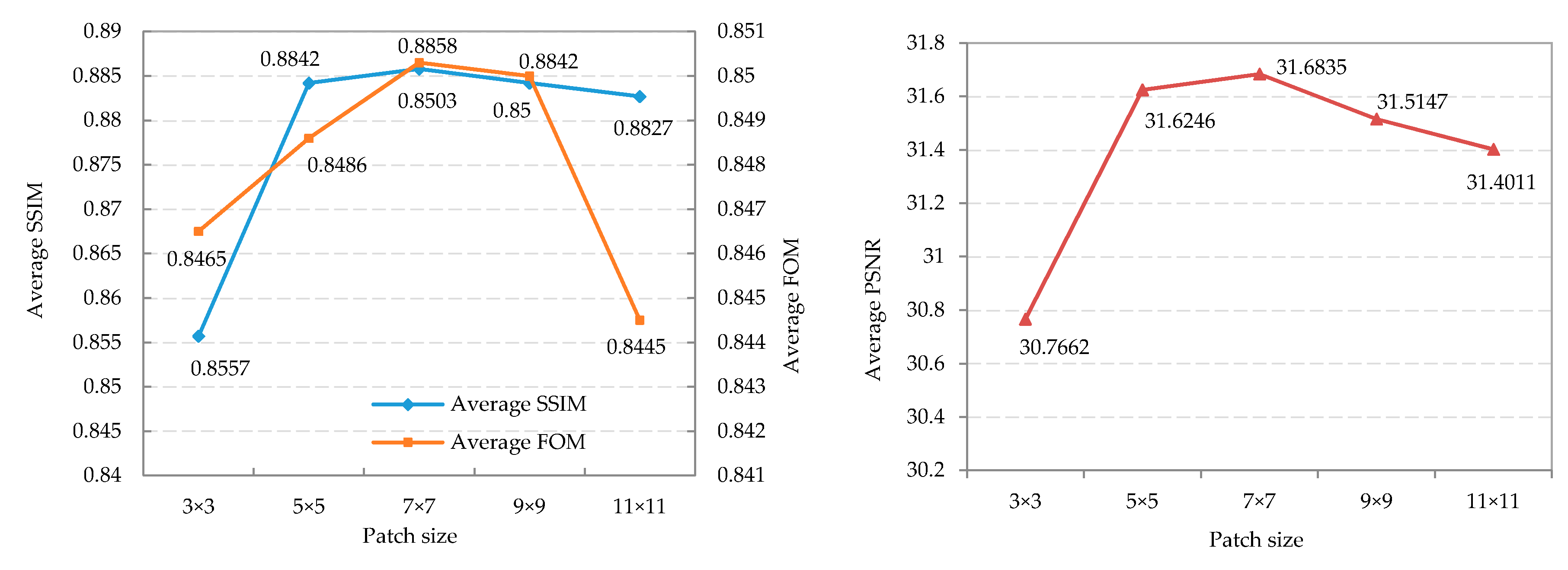
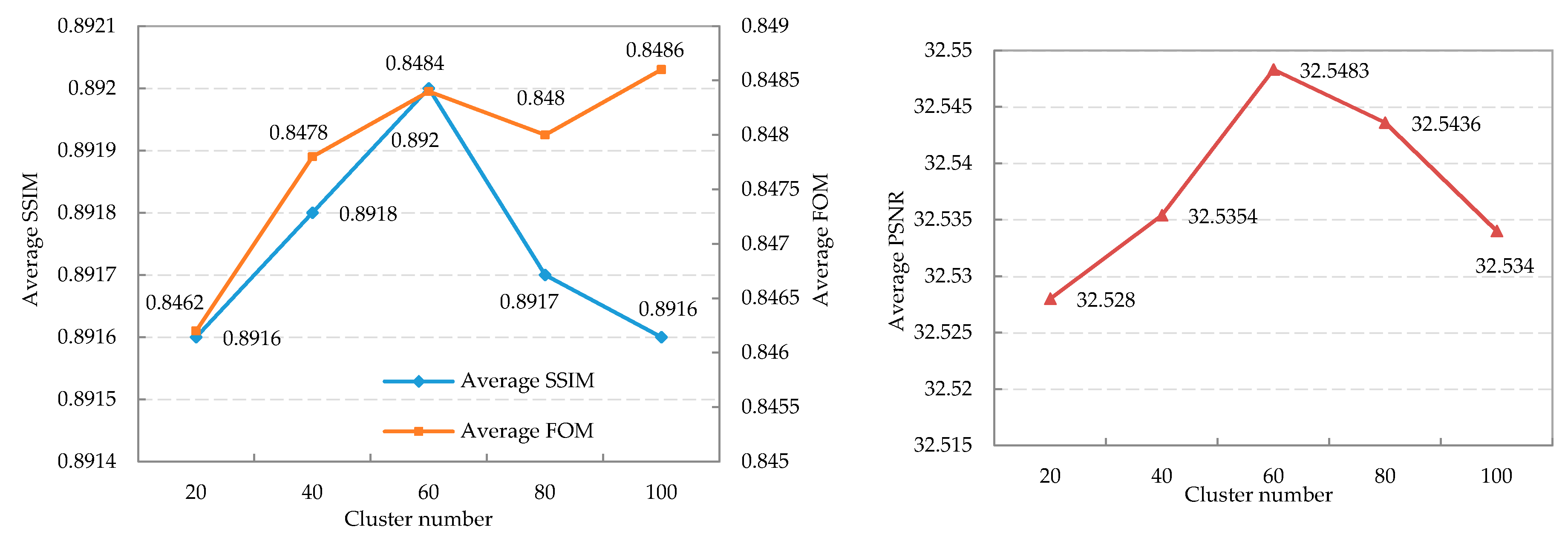
4.1. Parameters Setting

The parameters set in our experiment were as follows: the superpixels number $N_s$ was set to 500, the cluster number $K$ was set to 60, the patch size $b\times b$ was set to $7\times 7$, noise variance $\delta$ was in the range of $\left[5,15,25,40,60,80\right]$, and the number of similar patches $L$ was set to 10. The iteration number $J$ was set based on the noise level, and we required more iterations for a higher noise level. From experience, we set the iteration number $J$ to 7, 9, 13 and 16 for $\delta \le 15$, $15<\mathsf{\delta }\le 30$, $30<\mathsf{\delta }\le 60$ and $\mathsf{\delta }\ge 60$, respectively. Other regularity parameters were all empirical values as well, where β was set to 0.5, $\rho$ was set to 0.5, $\mu$ was set to 0.01, $\gamma$ was set to 0.2, $\lambda$ was set to 0.03, $\eta$ was set to 0.3 [15,16].

To verify the influence of image patch size $b\times b$ on peak signal to noise ratio (PSNR), structural similarity (SSIM), figure of merit (FOM), 100 test images were selected to calculate the average PSNR, average SSIM and average FOM with different patch size, when noise variance $\delta$ was set to 15. Figure 4 shows the changing trend of the average PSNR, average SSIM and average FOM over the image patch size. It was evident that when the patch size was equal to $7\times 7$, the average PSNR, average SSIM and average FOM achieved their maximum values. The influence of the cluster number $K$ on PSNR, SSIM and FOM was tested in the same way, and is shown in Figure 5. When the cluster number was equal to 60, the average PSNR and average FOM achieved their maximum values, and the average SSIM obtained its maximum values when the cluster number equaled to 100. To compromise, we set the cluster number $K$ to 60 for an optimal solution.

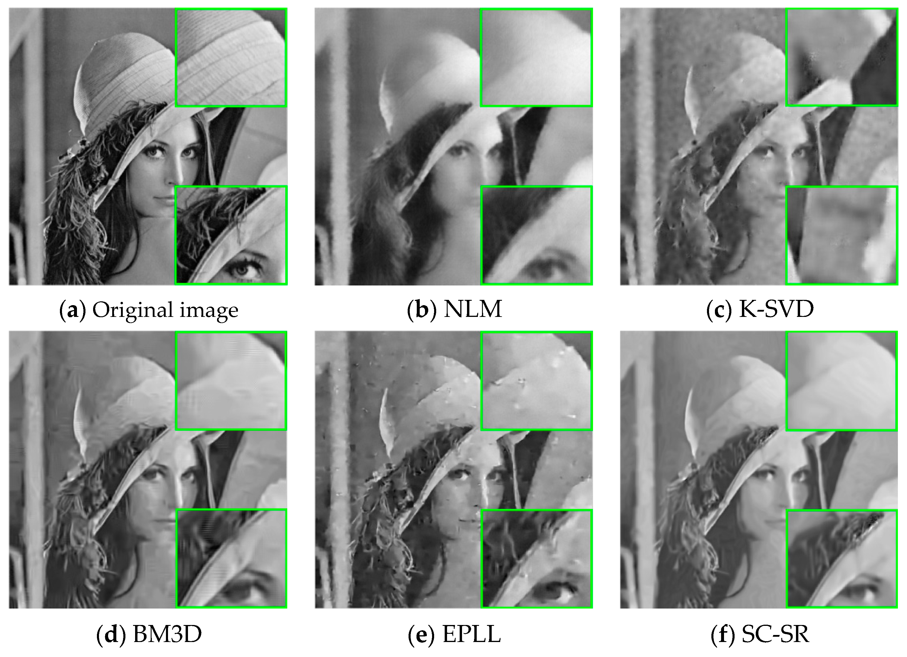
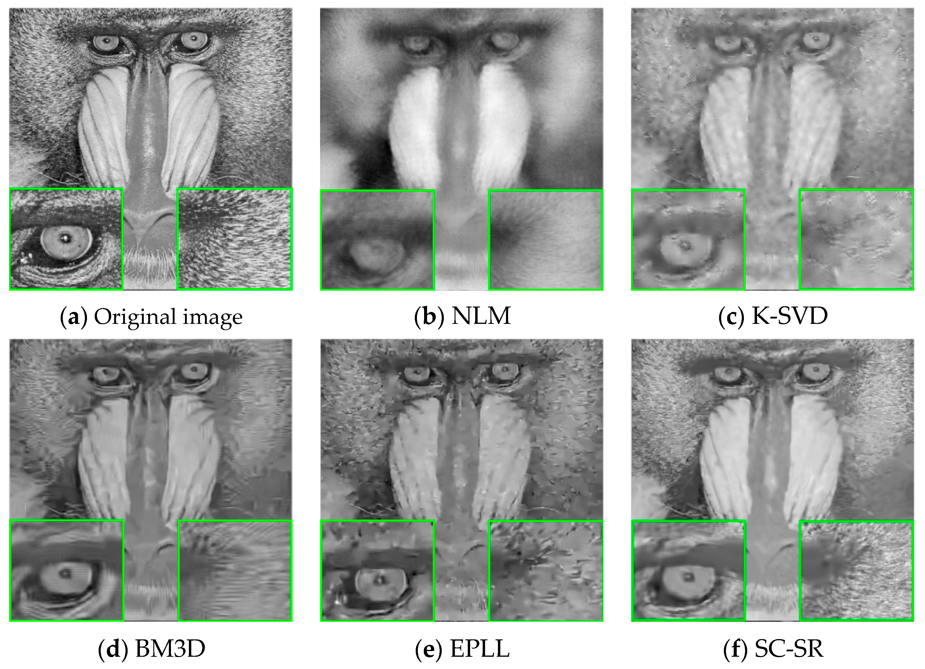
4.2. Qualitative Comparisons

Considering that human subjects are the ultimate judges of image quality, the visual quality of the denoised images is critical when evaluating a denoising algorithm. Figure 6 shows the noise-corrupted images of Monarch, Airplane, Lena and Baboon, whose noise variances were 25, 25, 60 and 60, respectively. Figure 7, Figure 8, Figure 9 and Figure 10 show the denoised images of Monarch, Airplane, Lena and Baboon disposed by competing algorithms. BM3D and NLM tended to over-smooth the image, while K-SVD BM3D and EPLL were likely to generate artifacts when noise was high. Due to the learned NSS prior by superpixel clustering, the proposed algorithm was more robust against artifacts, and preserved the edge and texture areas better than the other algorithms. For example, in the Monarch image, the SC-SR preserved the edges of the veins on the butterfly’s wings much better than the other algorithms. In the Airplane image, the SC-SR reconstructed the English alphabet on the wing of the aircraft more clearly than the other algorithms. In the Lena image, the SC-SR recovered more textures and edges on the hat than the other algorithms. In the Baboon image, the SC-SR preserved more fine texture of the hair of the baboon than other competing algorithms.

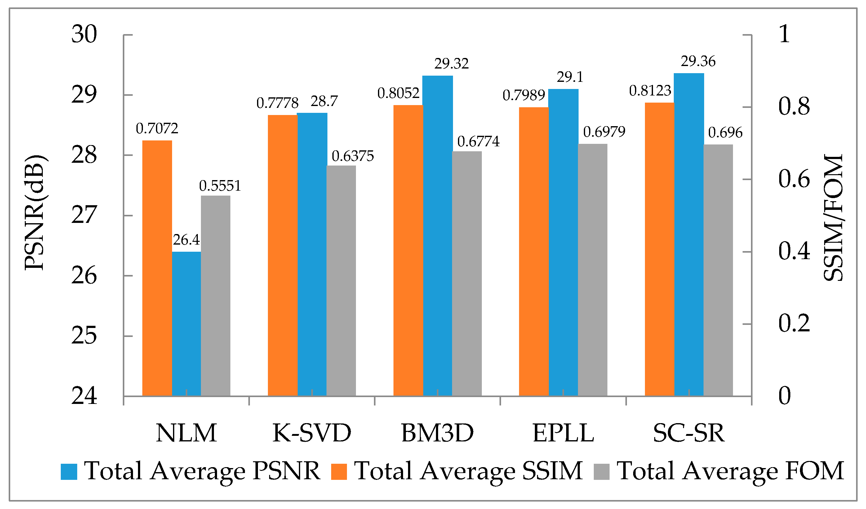
4.3. Quantitative Comparisons

To further validate the denoising capability of the proposed algorithm, we selected PSNR, SSIM and FOM as indexes to quantitatively evaluate the performance of the SC-SR algorithm. PSNR is one of the most widely used image objective evaluation indexes, and is able to measure the similarity of grayscale information between the original image and the denoised image. Since PSNR is based only on the error between the corresponding pixels, it cannot comprehensively describe structural similarity and the degree of edge preservation. SSIM is capable of assessing structural similarity, and FOM can be used to measure the degree of edge preservation between the original image and the denoised image.

Table 1. The PSNR, SSIM and FOM results for different denoising algorithms. Best results are in bold.

Images	(a) $\mathsf{\delta }=5$
	NLM	KSVD	BM3D	EPLL	SC-SR
Baboon	34.48	35.44	35.49	35.49	35.49
	0.9288	0.9536	0.9534	0.9552	0.9519
	0.9123	0.9326	0.9297	0.9332	0.9351
Fingerprint	34.44	36.63	36.51	36.43	36.65
	0.9807	0.9878	0.9876	0.9875	0.9887
	0.9056	0.8919	0.9876	0.9038	0.9642
Airplane	37.40	39.07	39.25	39.21	39.31
	0.9425	0.9584	0.9595	0.9604	0.9598
	0.9278	0.9251	0.9331	0.9372	0.9388
Monarch	36.72	37.74	38.25	38.27	38.29
	0.9677	0.9720	0.9756	0.9755	0.9758
	0.9789	0.9738	0.9762	0.9771	0.9751
Lena	37.17	38.62	38.71	38.59	38.74
	0.9239	0.9455	0.9444	0.9449	0.9450
	0.9113	0.9125	0.9303	0.9281	0.9289
House	37.34	39.43	39.86	38.97	39.94
	0.9164	0.9546	0.9568	0.9498	0.9584
	0.9383	0.9468	0.9535	0.9395	0.9442
Peppers	36.70	37.81	38.10	37.98	38.15
	0.9409	0.9550	0.9558	0.9562	0.9551
	0.9361	0.9378	0.9407	0.9508	0.9506
Straw	34.40	35.49	35.43	35.36	35.52
	0.9813	0.9850	0.9848	0.9846	0.9864
	0.9200	0.9218	0.9198	0.9143	0252
Hill	35.53	37.00	37.13	37.03	37.18
	0.9085	0.9423	0.9427	0.9437	0.9431
	0.8740	0.9181	0.9266	0.9216	0.9256
Woman	36.06	37.26	37.45	37.33	37.42
	0.9056	0.9336	0.9325	0.9347	0.9329
	0.9104	0.9291	0.9343	0.9306	0.9331
Average	36.024	37.449	37.62	37.47	37.67
	0.9396	0.95878	0.9593	0.9593	0.9597
	0.9215	0.92895	0.9432	0.9336	0.9421
Images	(b) $\mathsf{\delta }=15$
	NLM	KSVD	BM3D	EPLL	SC-SR
Baboon	25.95	28.42	28.67	28.70	28.77
	0.6800	0.8227	0.8327	0.8421	0.8388
	0.7051	0.8234	0.8187	0.8117	0.7995
Fingerprint	27.67	30.06	30.29	29.82	30.41
	0.8935	0.9462	0.9495	0.9462	0.9510
	0.6968	0.7075	0.7760	0.7761	0.7946
Airplane	31.31	33.60	33.89	33.78	33.97
	0.8756	0.9100	0.9162	0.9163	0.9163
	0.7677	0.8095	0.8240	0.8540	0.8482
Monarch	29.73	31.45	31.97	32.06	32.10
	0.8999	0.9282	0.9384	0.9379	0.9407
	0.9016	0.9226	0.9281	0.9397	0.9386
Lena	31.45	33.73	34.25	33.84	34.12
	0.8454	0.8860	0.8953	0.8893	0.8928
	0.6457	0.7552	0.7920	0.8185	0.8093
House	32.64	34.34	34.96	34.12	35.02
	0.8561	0.8778	0.8901	0.8768	0.8922
	0.7430	0.8541	0.8878	0.8749	0.8769
Peppers	30.23	32.25	32.69	32.55	32.64
	0.8624	0.8998	0.9064	0.9054	0.9050
	0.8123	0.8260	0.8408	0.8869	0.8661
Straw	26.67	28.57	28.65	28.53	28.72
	0.8661	0.9270	0.9291	0.9281	0.9350
	0.6833	0.7960	0.8049	0.8060	0.7952
Hill	28.89	31.45	31.85	31.69	31.88
	0.7270	0.8227	0.8394	0.8382	0.8428
	0.5812	0.7682	0.7800	0.8013	0.7959
Woman	29.91	31.92	32.42	32.23	32.38
	0.7860	0.8433	0.8545	0.8537	0.8543
	0.6355	0.7834	0.8018	0.8363	0.8323
Average	29.45	31.58	31.96	31.73	32.00
	0.8292	0.8864	0.8952	0.8934	0.8969
	0.7172	0.8046	0.8254	0.8405	0.8357
Images	(c) $\mathsf{\delta }=25$
	NLM	KSVD	BM3D	EPLL	SC-SR
Baboon	22.85	25.79	26.04	26.18	26.13
	0.4955	0.7081	0.7300	0.7483	0.7300
	0.4036	0.7245	0.7174	0.7245	0.7403
Fingerprint	24.32	27.30	27.72	27.14	27.79
	0.7979	0.8984	0.9117	0.9050	0.9117
	0.5974	0.6371	0.7034	0.6772	0.7321
Airplane	28.17	30.97	31.44	31.27	31.45
	0.8286	0.8719	0.8833	0.8794	0.8865
	0.6036	0.7306	0.7419	0.7904	0.7638
Monarch	26.43	28.72	29.31	29.33	29.44
	0.8336	0.8880	0.9031	0.9001	0.9045
	0.8066	0.8532	0.8821	0.9024	0.9076
Lena	28.73	31.34	32.05	31.59	31.98
	0.7964	0.8428	0.8607	0.8502	0.8615
	0.4242	0.6420	0.6885	0.7259	0.7178
House	29.08	32.09	32.93	32.13	32.96
	0.8114	0.8452	0.8595	0.8471	0.8604
	0.5850	0.7751	0.8319	0.8077	0.8202
Peppers	26.79	29.68	30.21	30.07	30.18
	0.8023	0.8564	0.8687	0.8652	0.8668
	0.6232	0.7385	0.7617	0.8168	0.791
Straw	21.98	25.71	25.92	25.80	25.90
	0.6225	0.8509	0.8631	0.8607	0.8739
	0.6160	0.7132	0.7162	0.7001	0.7155
Hill	26.41	29.22	29.81	29.61	29.83
	0.6400	0.7406	0.7748	0.7688	0.7721
	0.3723	0.6441	0.6607	0.6947	0.6723
Woman	27.14	29.66	30.29	30.04	30.25
	0.7245	0.7853	0.8069	0.7995	0.8053
	0.4585	0.6492	0.6854	0.7579	0.6990
Average	26.19	29.05	29.57	29.32	29.59
	0.7353	0.8288	0.8462	0.8424	0.8473
	0.5490	0.7108	0.7389	0.7598	0.7560
Images	(d) $\mathsf{\delta }=40$
	NLM	KSVD	BM3D	EPLL	SC-SR
Baboon	21.65	23.57	23.88	24.03	24.01
	0.4072	0.5570	0.6029	0.6189	0.6057
	0.2764	0.5428	0.5252	0.5865	0.5758
Fingerprint	21.31	24.71	25.29	24.72	25.45
	0.6613	0.8179	0.8587	0.8433	0.8563
	0.5515	0.6274	0.6179	0.5513	0.6536
Airplane	25.32	28.53	29.06	28.98	29.13
	0.7797	0.8231	0.8401	0.8335	0.8515
	0.4750	0.6135	0.6570	0.7161	0.6792
Monarch	23.12	26.56	26.72	27.03	26.77
	0.7517	0.8344	0.8485	0.8487	0.8521
	0.6844	0.8143	0.8259	0.8537	0.8128
Lena	26.53	29.06	29.86	29.43	29.92
	0.7511	0.7928	0.8159	0.8005	0.8253
	0.3266	0.4858	0.5677	0.6164	0.5769
House	25.96	29.59	30.64	29.74	30.71
	0.7569	0.7996	0.8256	0.8020	0.8356
	0.4821	0.6676	0.7350	0.7058	0.7229
Peppers	23.71	27.33	27.79	27.59	27.68
	0.7328	0.8046	0.8181	0.8134	0.8223
	0.4603	0.6523	0.6862	0.7412	0.6686
Straw	19.66	22.93	23.19	23.28	23.38
	0.4039	0.6928	0.7435	0.7397	0.7425
	0.5265	0.5529	0.5933	0.5560	0.5950
Hill	24.71	27.15	27.93	27.76	28.05
	0.5766	0.6562	0.7053	0.6963	0.7039
	0.2446	0.4413	0.5207	0.5629	0.5388
Woman	25.01	27.61	28.31	28.08	28.38
	0.6722	0.7258	0.7501	0.7383	0.7556
	0.3546	0.5039	0.5578	0.6506	0.5694
Average	23.70	26.70	27.27	27.06	27.35
	0.6493	0.7504	0.7809	0.7735	0.7851
	0.4382	0.5902	0.6287	0.6541	0.6393
Images	(e) $\mathsf{\delta }=60$
	NLM	KSVD	BM3D	EPLL	SC-SR
Baboon	20.95	22.08	22.38	22.48	22.56
	0.3568	0.4356	0.4685	0.4890	0.4901
	0.2680	0.3077	0.3173	0.4114	0.4358
Fingerprint	18.95	21.77	23.59	22.65	23.63
	0.4952	0.6804	0.7974	0.7597	0.7900
	0.5073	0.4908	0.5027	0.4514	0.5731
Airplane	23.27	26.01	27.01	26.95	27.13
	0.7273	0.7602	0.7860	0.7767	0.8163
	0.3625	0.4633	0.5389	0.6253	0.5881
Monarch	20.43	24.22	24.58	24.72	24.81
	0.6503	0.7618	0.7777	0.7795	0.8006
	0.5406	0.7315	0.7300	0.7614	0.7472
Lena	24.59	26.90	27.98	27.60	28.05
	0.6999	0.7328	0.7636	0.7465	0.7871
	0.2777	0.3298	0.4394	0.5013	0.4753
House	23.59	26.75	28.49	27.90	28.53
	0.6967	0.7252	0.7768	0.7636	0.7669
	0.3941	0.4638	0.6288	0.6379	0.6204
Peppers	21.15	25.02	25.51	25.67	25.45
	0.6634	0.7386	0.7479	0.7621	0.7717
	0.3990	0.5282	0.5401	0.6354	0.5801
Straw	18.59	20.51	21.26	20.99	21.39
	0.2785	0.4726	0.5824	0.5521	0.5970
	0.4419	0.4592	0.4804	0.4240	0.4837
Hill	23.54	25.61	26.35	26.20	26.29
	0.5283	0.5928	0.6332	0.6262	0.6355
	0.2153	0.2665	0.4002	0.4424	0.4223
Woman	23.47	25.86	26.55	26.43	26.49
	0.6251	0.6701	0.6948	0.6810	0.7063
	0.3299	0.3405	0.4232	0.5175	0.4604
Average	21.85	24.47	25.37	25.16	25.43
	0.5722	0.6570	0.7028	0.6936	0.7162
	0.3736	0.4381	0.5001	0.5408	0.5386
Images	(f) $\mathsf{\delta }=80$
	NLM	KSVD	BM3D	EPLL	SC-SR
Baboon	20.68	21.40	21.64	21.68	21.71
	0.3379	0.3860	0.4049	0.4186	0.4137
	0.2387	0.2205	0.2224	0.2889	0.2988
Fingerprint	17.75	19.55	22.39	21.12	22.39
	0.3781	0.5355	0.7478	0.6770	0.7347
	0.4376	0.4397	0.4699	0.3869	0.4956
Airplane	22.05	24.18	25.54	25.61	25.63
	0.6723	0.6981	0.7453	0.7292	0.7902
	0.3280	0.3511	0.4741	0.5509	0.5399
Monarch	22.52	22.52	23.20	23.42	23.29
	0.5569	0.7050	0.7237	0.7313	0.7553
	0.4911	0.6201	0.6733	0.7203	0.6947
Lena	23.41	25.44	26.65	26.14	26.71
	0.6597	0.6846	0.7225	0.6952	0.7568
	0.2670	0.2793	0.3720	0.4114	0.3997
House	22.29	24.80	26.94	26.22	26.74
	0.6442	0.6584	0.7379	0.7098	0.7669
	0.3322	0.3521	0.5329	0.5557	0.5204
Peppers	19.78	22.97	24.12	24.19	24.06
	0.6038	0.6710	0.7006	0.7103	0.7391
	0.3690	0.4105	0.4783	0.5880	0.5396
Straw	18.21	19.22	19.94	19.80	20.01
	0.2248	0.3306	0.4410	0.4210	0.4584
	0.3582	0.3758	0.3812	0.3344	0.4187
Hill	22.84	24.66	25.28	25.19	25.23
	0.4993	0.5544	0.5865	0.5784	0.5967
	0.1925	0.2137	0.3179	0.3352	0.3349
Woman	22.58	24.55	25.39	25.29	25.24
	0.5967	0.6279	0.6551	0.6419	0.6739
	0.2998	0.2612	0.3610	0.4118	0.3976
Average	21.21	22.93	24.10	23.87	24.11
	0.5174	0.5852	0.6465	0.6313	0.6686
	0.3314	0.3524	0.4283	0.4584	0.4640

presents the PSNR, SSIM and FOM results for different algorithms, images, and noise variances. As presented in Table 1, the top value is the PSNR result, the middle value is the SSIM result, and the bottom value is the FOM result in every table cell.

From Table 1, we could observe three points. Firstly, the proposed SC-SR algorithm achieved much better PSNR, SSIM and FOM results than NLM and K-SVD in all cases. Secondly, SC-SR had higher PSNR and SSIM values than EPLL in most cases. Moreover, EPLL acquired the best FOM results among the five algorithms, and SC-SR was only slightly inferior to EPLL. Thirdly, SC-SR obtained better SSIM and FOM results than BM3D in most cases. Meanwhile, when the noise variance was low, the PSNR results of SC-SR were close to BM3D; when the noise variance was high, the PSNR results of SC-SR were obviously better than BM3D, since BM3D trended to suffer from artifacts in this case. According to the these points, we can come to the conclusion that SC-SR is capable of stronger comprehensive ability in reservation of structural, edge and grayscale information and does better in denoising images in comparison with the other algorithms. In order to further testify the conclusions, we made a mean processing for the data results in Table 1, and showed the result in Figure 11.

In Figure 11, we demonstrated the total averages of the PSNR, SSIM and FOM for NLM, K-SVD, BM3D, EPLL and SC-SR. For each algorithm, the total average PSNR was calculated by the mean of the average PSNR results with different noise variances (Table 1), and the total average SSIM and the total average FOM were calculated in the same way. As seen in Figure 11, it was obvious that SC-SR achieved the highest total average PSNR and total average SSIM, while EPLL attained the highest total average FOM. SC-SR was close to EPLL and higher than BM3D for the total average FOM. BM3D had a similar total average PSNR as SC-SR, but a lower total average SSIM and total average FOM than SC-SR. EPLL had higher total average FOM, but lower total average PSNR and total average SSIM than SC-SR and BM3D. In brief, among the five algorithms, BM3D possessed the best capacity for removing noise and preserving structural information, and the second-best capacity for preserving edge areas. In general, SC-SR could not only effectively remove the noise, but also preserve the image edge regions and structural information in the round.

All experiments were run under the MATLAB 2014a environment on a machine with Intel(R) Xeon(R) E5-2690 CPU of 2.60 GHz and 96.0 GB RAM. Owing to compiled C++ mex-function and parallelization implementation, BM3D proved to be the fastest algorithm. Furthermore, NLM benefited from compiled C++ mex-function, and turned into the second-fastest algorithm. Other algorithms suffered from high computational cost based on their computation complexity, as well as their implementation, which simply uses C language with MATLAB. The test revealed that EPLL was about two times slower than K-SVD, and SC-SR suffered from slightly higher computational costs than EPLL due to the involvement of several subtasks and iterative shrinkage operations. However, several accelerating techniques, such as the accelerating techniques described in References [23], could be used to accelerate the convergence of the proposed algorithm. Additionally, the compiled C++ mex-function and parallelization implementation could be adopted to dispose of multiple subtasks to improve the speed of the proposed algorithm. Hence, the computational costs of the proposed algorithm can be further reduced.

5. Conclusions

In this paper, we presented a new image denoising algorithm which made full use of image priors, including the NSS prior in the spatial domain and sparse transform domain, edges and structural information, and sparsity. It was accomplished in two successive steps based on superpixel clustering and sparse representation. First, we learned the NSS prior in mid-level vision by clustering superpixels. Since superpixel clustering takes edge and structural information into account, a better exploitation of the NSS prior could be obtained. Meanwhile, multiple features were selected to describe a superpixel in the clustering process, which also facilitated a good NSS prior. Second, we took advantage of the NSS prior in the sparse transform domain by using a weighted average sparse coefficient from similar patches to improve the effectiveness of the sparse coefficient for each patch. Experiments conducted on a collection of standard test images demonstrated that the proposed algorithm not only effectively removed the noise, but also provided a better restoration of both the structural information and the edge region algorithms, and overall produced less visual artifacts than other competing algorithms.

References

1. Buades, A.; Coll, B.; Morel, J.M. A non-local algorithm for image denoising. In Proceedings of the International Conference on Computer Vision and Pattern Recognition (CVPR), San Diego, CA, USA, 20–25 June 2005. [Google Scholar]
2. Dabov, K.; Foi, A.; Katkovnik, V.; Egiazarian, K. Image denoising by sparse 3-D transform-domain collaborative filtering. IEEE Trans. Image Process. 2007, 16, 2080–2095. [Google Scholar] [CrossRef] [PubMed]
3. Elad, M.; Aharon, M. Image denoising via sparse and redundant representations over learned dictionaries. IEEE Trans. Image Process. 2006, 15, 3736–3745. [Google Scholar] [CrossRef] [PubMed]
4. Aharon, M.; Elad, M.; Bruckstein, A. The K-SVD: An algorithm for designing overcomplete dictionaries for sparse representation. IEEE Trans. Signal Process. 2006, 54, 4311–4322. [Google Scholar] [CrossRef]
5. Mairal, J.; Bach, F.; Ponce, J.; Sapiro, G.; Zisserman, A. Non-local sparse models for image restoration. In Proceedings of the IEEE International Conference on Computer Vision (ICCV), Kyoto, Japan, 27 September–4 October 2009. [Google Scholar]
6. Chatterjee, P.; Milanfar, P. Clustering-Based Denoising with locally learned dictionaries. IEEE Trans. Image Process. 2009, 18, 1438–1451. [Google Scholar] [CrossRef] [PubMed]
7. Dong, W.S.; Zhang, L.; Shi, G.M.; Li, X. Nonlocally centralized sparse representation for image restoration. IEEE Trans. Image Process. 2013, 22, 1620–1630. [Google Scholar] [CrossRef] [PubMed]
8. Gu, S.H.; Zhang, L.; Zuo, W.M.; Feng, X.C. Weighted nuclear norm minimization with application to image denoising. In Proceedings of the International Conference on Computer Vision and Pattern Recognition (CVPR), Columbus, OH, USA, 23–28 June 2014. [Google Scholar]
9. Ji, H.; Liu, C.Q.; Shen, Z.W.; Xu, Y.H. Robust video denoising using low rank matrix completion. In Proceedings of the IEEE International Conference on Computer Vision and Pattern Recognition (CVPR), San Francisco, CA, USA, 13–18 June 2010. [Google Scholar]
10. Xu, J.; Zhang, L.; Zuo, W.M.; Zhang, D.; Feng, X.C. Patch Group Based Nonlocal Self-Similarity Prior Learning for Image Denoising. In Proceedings of the IEEE International Conference on Computer Vision (ICCV), Santiago, Chile, 7–13 December 2015. [Google Scholar]
11. Achanta, R.; Shaji, A.; Smith, K.; Lucchi, A.; Fua, P.; Susstrunk, S. SLIC Superpixels Compared to State-of-the-Art Superpixel Methods. IEEE Trans. Pattern Anal. 2012, 34, 2274–2282. [Google Scholar] [CrossRef] [PubMed]
12. Achanta, R.; Shaji, A.; Smith, K.; Lucchi, A.; Fua, P.; Susstrunk, S. SLIC Superpixels; EPFL Technical Report No. 149300; EPFL: Lausanne, Switzerland, 2010. [Google Scholar]
13. Elhamifar, E.; Vidal, R. Sparse subspace clustering. In Proceedings of the International Conference on Computer Vision and Pattern Recognition (CVPR), Miami, FL, USA, 20–25 June 2009. [Google Scholar]
14. Tibshirani, R. Regression shrinkage and selection via the lasso. J. R. Stat. Soc. B 1996, 58, 267–288. [Google Scholar]
15. Xie, Y.; Lu, H.; Yang, M.H. Bayesian Saliency via Low and Mid-Level Cues. IEEE Trans. Image Process. 2013, 22, 1689–1698. [Google Scholar] [PubMed]
16. Dong, W.S.; Zhang, L.; Shi, G.M.; Wu, X.L. Image Deblurring and Super-resolution by Adaptive Sparse Domain Selection and Adaptive Regularization. IEEE Trans. Image Process. 2011, 20, 1838–1857. [Google Scholar] [CrossRef] [PubMed]
17. Zhang, L.; Dong, W.; Zhang, D.; Shi, G.M. Two-stage image denoising by principal component analysis with local pixel grouping. IEEE Trans. Image Process. 2010, 43, 1531–1549. [Google Scholar] [CrossRef]
18. Wang, J.; Kwon, S.; Shim, B. Generalized orthogonal matching pursuit. IEEE Trans. Signal Process. 2012, 60, 6202–6216. [Google Scholar] [CrossRef]
19. Daubechies, I.; Defriese, M.; Mol, C.D. An iterative thresholding algorithm for linear inverse problems with a sparsity constraint. Commun. Pure Appl. Math. 2004, 57, 1413–1457. [Google Scholar] [CrossRef]
20. Dong, W.S.; Li, X.; Zhang, L.; Shi, G.M. Sparsity-based Image Denoising via Dictionary Learning and Structural Clustering. In Proceedings of the International Conference on Image Processing (ICIP), Brussels, Belgium, 11–14 September 2011. [Google Scholar]
21. Zoran, D.; Weiss, Y. From learning models of natural image patches to whole image restoration. In Proceedings of the IEEE International Conference on Computer Vision (ICCV), Barcelona, Spain, 6–13 November 2011. [Google Scholar]
22. Gao, X.; Lu, W.; Tao, D.; Li, X. Image quality assessment based on multiscale geometric analysis. IEEE Trans. Image Process. 2009, 18, 1409–1423. [Google Scholar] [PubMed]
23. Beck, A.; Teboulle, M. A fast iterative shrinkage thresholding algorithm for linear inverse problems. SIAM J. Imaging Sci. 2009, 2, 183–202. [Google Scholar] [CrossRef]
Figure 1. Segmentation results of simple linear iterative clustering (SLIC).
Applsci 07 00436 g001
Figure 2. Matrix mirroring extension.
Applsci 07 00436 g002
Figure 3. The 10 standard benchmark images. (a) Baboon; (b) Fingerprint; (c) Airplane; (d) Monarch; (e) Lena; (f) House; (g) Peppers; (h) Straw; (i) Hill; (j) Woman.
Applsci 07 00436 g003
Figure 4. The impact of patch size on average PSNR (peak signal to noise ratio), average SSIM (structural similarity), and average FOM (figure of merit) of SC-SR.
Applsci 07 00436 g004
Figure 5. The impact of cluster number on average PSNR, average SSIM, and average FOM of SC-SR.
Applsci 07 00436 g005
Figure 6. The four noise-destroyed images.
Applsci 07 00436 g006
Figure 7. Comparison of denoising results of the Monarch noisy image corrupted by additive white Gaussian noise δ = 25 : (a) Original image; (b) nonlocal means (NLM): PSNR = 26.43   dB , SSIM = 0.8336 , FOM = 0.8066 ; (c) K-SVD: PSNR = 28.72   dB , SSIM = 0.8880 , FOM = 0.8532 ; (d) block-matching and 3D filtering (BM3D): PSNR = 29.38   dB , SSIM = 0.9001 , FOM = 0.9024 ; (e) expected patch log likelihood (EPLL): PSNR = 29.38   dB , SSIM = 0.9001 , FOM = 0.9024 ; and (f) SC-SR: PSNR = 29.44   dB , SSIM = 0.9045 , FOM = 0.9076 .
Applsci 07 00436 g007
Figure 8. Comparison of denoising results of the Airplane noisy image corrupted by additive white Gaussian noise δ = 25 : (a) Original image; (b) NLM: PSNR = 28.17   dB , SSIM = 0.8286 , FOM = 0.6036 ; (c) K-SVD: PSNR = 30.97   dB , SSIM = 0.8719 , FOM = 0.7306 ; (d) BM3D: PSNR = 31.44   dB , SSIM = 0.8833 , FOM = 0.7419 ; (e) EPLL: PSNR = 31.27   dB , SSIM = 0.8794 , FOM = 0.7904 ; and (f) SC-SR: PSNR = 31.45   dB , SSIM = 0.8865 , FOM = 0.7638 .
Applsci 07 00436 g008
Figure 9. Comparison of denoising results of the Lena noisy image corrupted by additive white Gaussian noise δ = 60 : (a) Original image; (b) NLM: PSNR = 24.59   dB , SSIM = 0.6999 , FOM = 0.2777 ; (c) K-SVD: PSNR = 26.90   dB , SSIM = 0.7328 , FOM = 0.3298 ; (d) BM3D: PSNR = 27.98   dB , SSIM = 0.7636 , FOM = 0.4394 ; (e) EPLL: PSNR = 27.60   dB , SSIM = 0.7465 , FOM = 0.5013 ; and (f) SC-SR: PSNR = 28.05   dB , SSIM = 0.7871 , FOM = 0.4753 .
Applsci 07 00436 g009
Figure 10. Comparison of denoising results of the Baboon noisy image corrupted by additive white Gaussian noise δ = 60 : (a) Original image; (b) NLM: PSNR = 20.95   dB , SSIM = 0.3568 , FOM = 0.2680 ; (c) K-SVD: PSNR = 22.08   dB , SSIM = 0.4356 , FOM = 0.3077 ; (d) BM3D: PSNR = 22.38   dB , SSIM = 0.4685 , FOM = 0.3173 ; (e) EPLL: PSNR = 22.48   dB , SSIM = 0.4890 , FOM = 0.4114 , and (f) SC-SR: PSNR = 22.56   dB , SSIM = 0.4901 , FOM = 0.4358 .
Applsci 07 00436 g010
Figure 11. Comparison of the total average PSNR, total average SSIM and total average FOM for different denoising algorithms.
Applsci 07 00436 g011