
A Neural Parametric Singing Synthesizer Modeling Timbre and Expression from Natural Songs †


Abstract
:1. Introduction
2. Proposed System
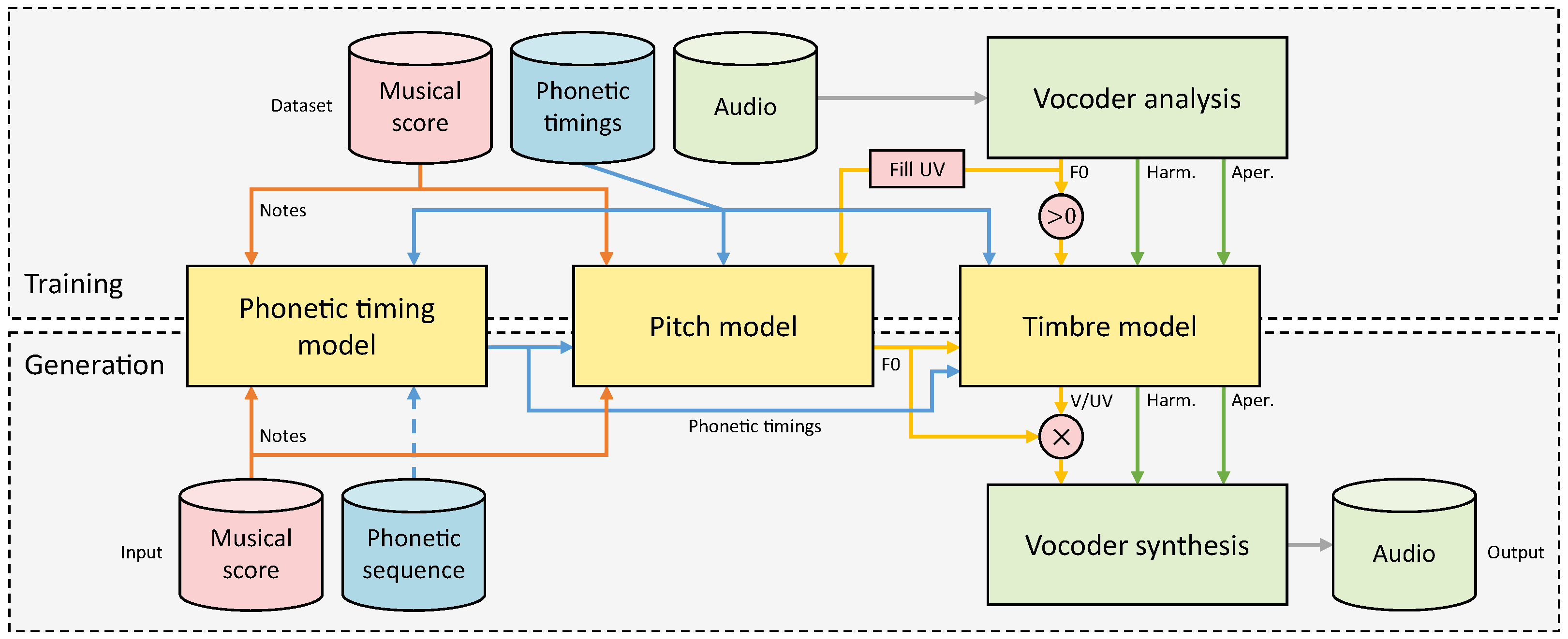
2.1. Overview
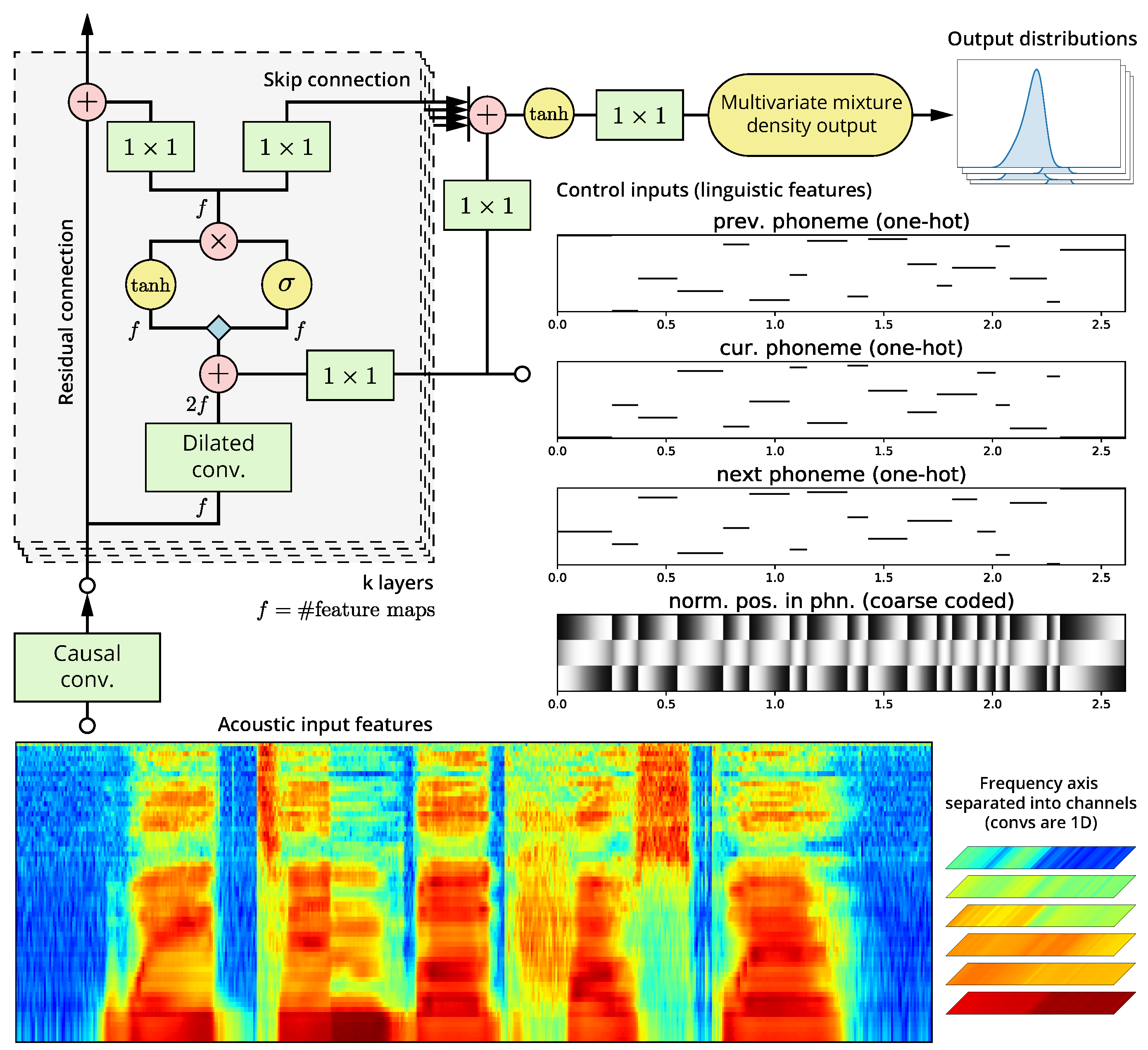
2.2. Modified WaveNet Architecture
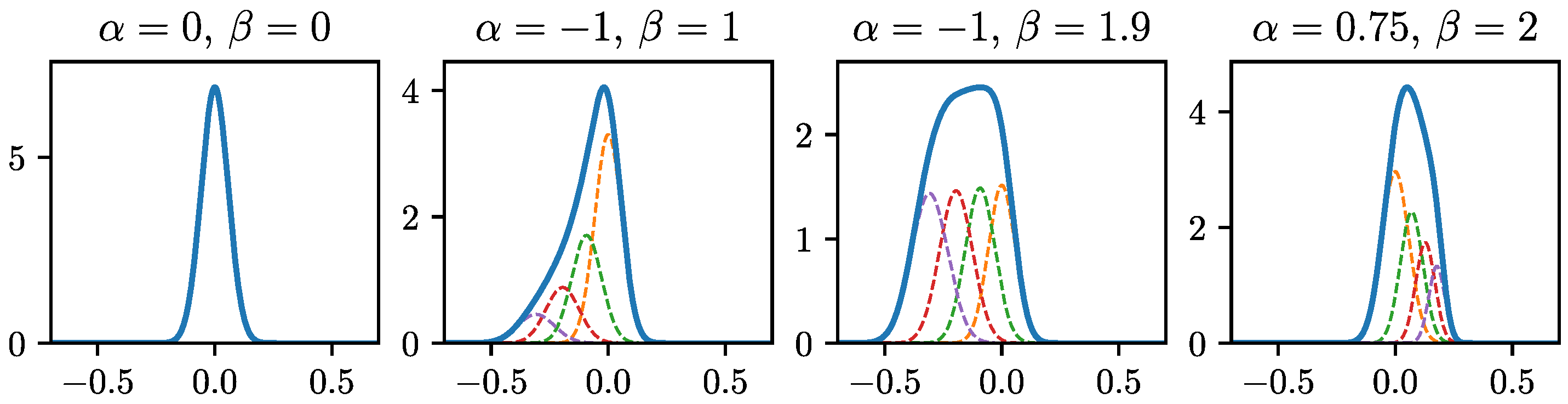
2.2.1. Constrained Mixture Density Output
2.2.2. Regularization
2.3. Timbre Model
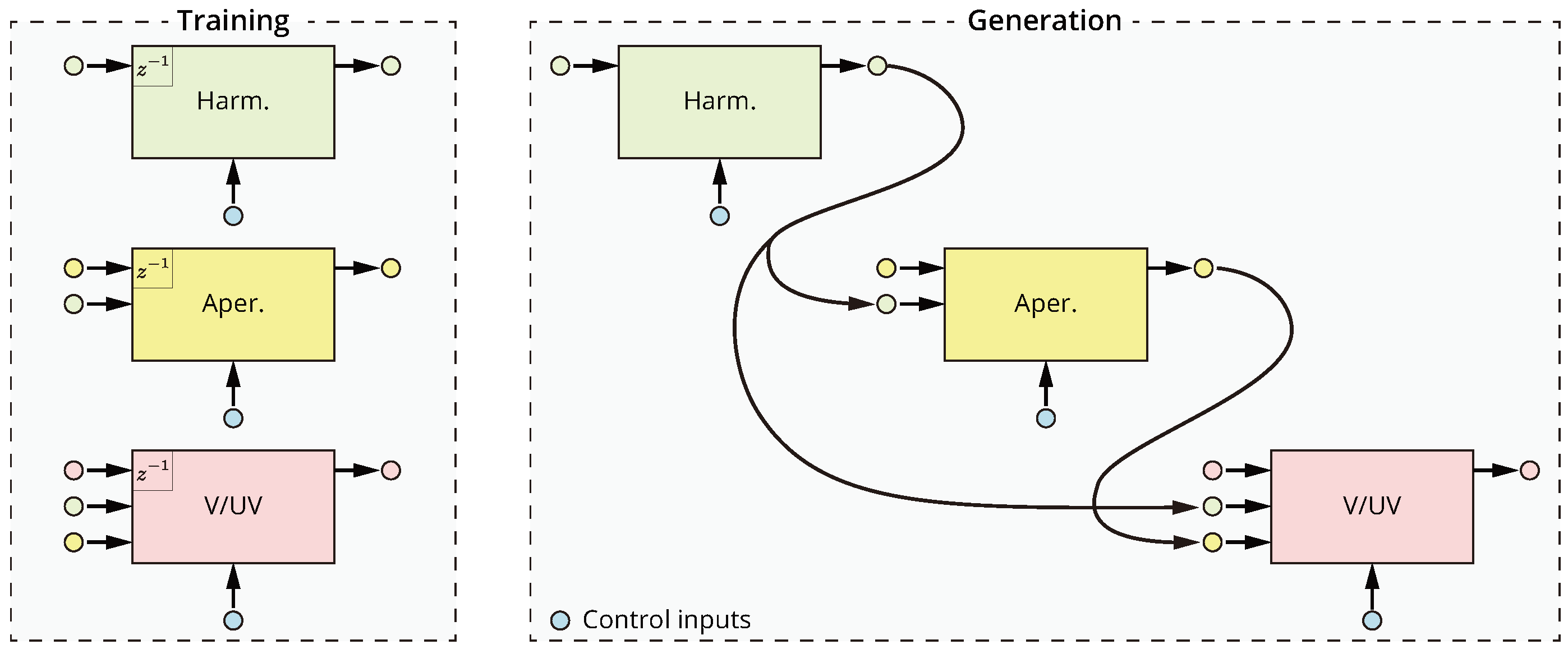
2.3.1. Multistream Architecture
2.3.2. Handling Long Notes
2.4. Pitch Model
2.4.1. Data Augmentation
2.4.2. Tuning Postprocessing
2.5. Timing Model
2.5.1. Note Timing Model
2.5.2. Phoneme Duration Model
2.5.3. Fitting Heuristic
2.6. Acoustic and Control Frontend
2.7. Audio Generation Speed
3. Related Work
4. Experiments
4.1. Datasets
4.2. Compared Systems
- NPSS: Our system, which we call Neural Parametric Singing Synthesizer (NPSS), as described in Section 2.
- IS16: A concatenative unit selection-based system [1], which was the highest rated system in the Interspeech 2016 Singing Synthesis Challenge.
- Sinsy-HMM: A publicly accessible implementation of the Sinsy HMM-based synthesizer (http://www.sinsy.jp/). This system is described in [4,35], although the implementation may differ to some degree from any single publication, according to one of the authors in private correspondence. While the system was trained on the same NIT-SONG070-F001 dataset, it should be noted that the full 70 song dataset was used, including the 3 songs we use for testing.
- Sinsy-DNN: A publicly accessible implementation of the Sinsy feedforward DNN-based synthesizer (http://www.sinsy.jp/) [37]. The same caveats as with Sinsy-HMM apply here. Additionally, the DNN voice is marked as “beta”, and thus should be considered still experimental. The prediction of timing and vibrato parameters in this system seems to be identical to Sinsy-HMM at the time of writing. Thus, only timbre and “baseline” F0 is predicted by the DNN system.
- HTS: A HMM-based system, similar to Sinsy-HMM, but consisting of a timbre model only, and trained on pseudo singing. The standard demo recipe from the HTS toolkit (version 2.3) [38] was followed, except for a somewhat simplified context dependency (just the two previous and two following phonemes).
4.3. Methodology
4.3.1. Quantitative Metrics
- Mel-Cepstral Distortion (MCD): Mel-Cepstral Distortion (MCD) is a common perceptually motivated metric for the quantitative evaluation of timbre models. In our case, some moderate modifications are made to improve robustness for singing voice; Mel-cepstral parameters are extracted from WORLD spectra, rather than STFT spectra, to better handle high pitches. To reduce the effect of pitch mismatches between reference and prediction, we filter pairs of frames with a pitch difference exceeding ±200 cents. Similarly, to increase robustness to small misalignments in time, frames with a modified z-score exceeding 3.5 are not considered [39]. MCD is computed for harmonic components, using 33 (0–13.6 kHz) coefficients.
- Band Aperiodicity Distortion (BAPD): Identical to MCD, except computed over linearly spaced band aperiodicity coefficients. BAPD is computed for aperiodic components, using 4 (3–12 kHz) coefficients.
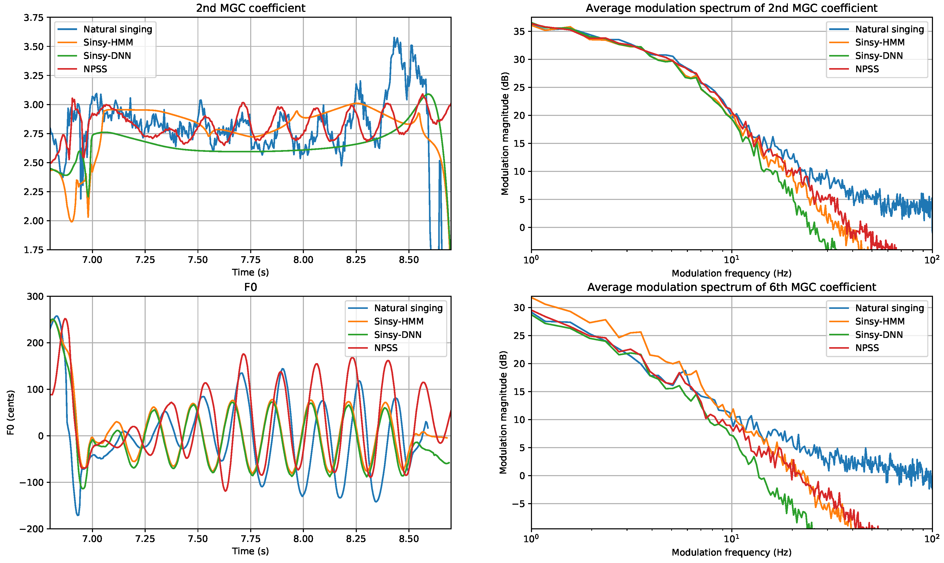
- Modulation Spectrum (MS) for Mel-Generalized Coefficients (MGC): One issue with framewise metrics, like MCD, is that these do not consider the behavior of the predicted parameter sequences over time. In particular, the common issue of oversmoothing is typically not reflected in these metrics. A recently proposed metric, the Modulation Spectrum (MS) [40], allows visualizing the spectral content of predicted time sequences. For instance, showing oversmoothing as a rolloff of higher modulation frequencies. We are mainly interested in the lower band of the MS (e.g., <25 Hz), because the higher band of the reference (natural singing) can be overly affected by noise in the parameter estimation. To obtain a single scalar metric, we use the Modulation Spectrum Log Spectral Distortion (MS-LSD) between the modulation spectra of a predicted parameter sequence and a reference recording.
- Voiced/unvoiced decision metrics: In singing voice, there is a notable imbalance between voiced and unvoiced frames due to having many long, sustained vowels. As both false positives (unvoiced frames predicted as voiced) and false negatives (voiced frames predicted as unvoiced) can result in highly noticeable artifacts, we list both False Positive Rate (FPR) and False Negative Rate (FPR) for this estimator. All silences are excluded.
- Timing metrics: Metrics for the timing model are relatively straight forward, e.g., Mean Absolute Error (MAE), Root Mean Squared Error (RMSE) or Pearson correlation coefficient r between onsets or durations. We list errors for note onsets, offsets and consonant durations separately to ensure the fitting heuristic affects the results only minimally.
- F0 metrics: Standard F0 metrics such as RMSE are given, but it should be noted that these metrics are often not very correlated to perceptual metrics in singing [41]. For instance, starting a vibrato slightly early or late compared to the reference may be equally valid musically, but can the cause the two F0 contours to become out of phase, resulting in high distances.
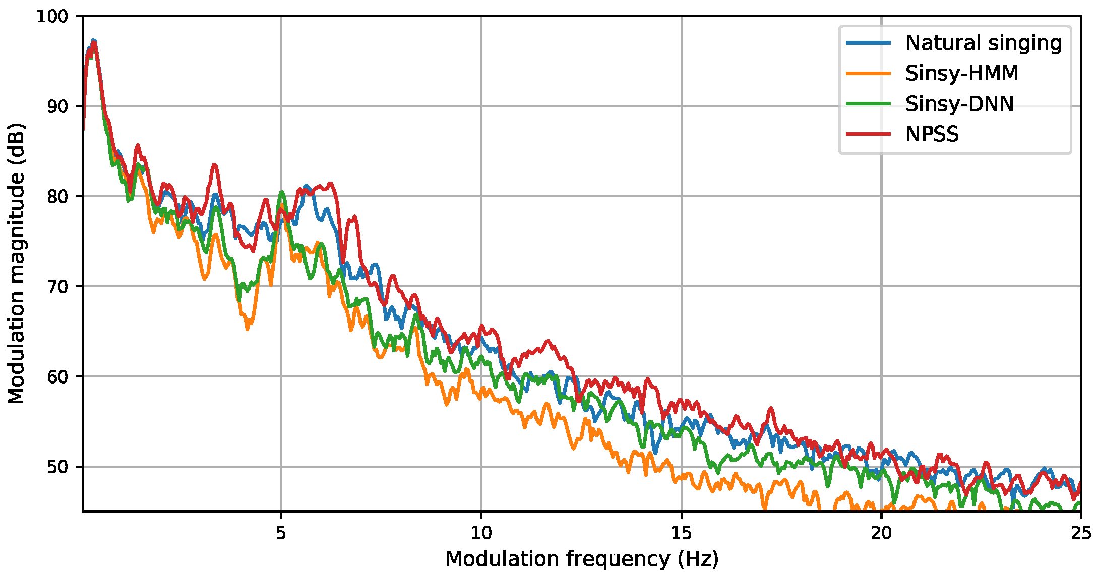
- Modulation Spectrum (MS) for log F0: Similar to timbre, we use MS-based metrics to get a sense of how close the generated F0 contours are in terms of variability over time. The MS of F0 is computed by first segmenting the score into sequences of continuous notes, without rests. Then, for each sequence, the remaining unvoiced regions in the log F0 curve are filled using cubic spline interpolation. We apply a Tukey window corresponding to a 50 frame fade in and fade out, and subtract the per-sequence mean. Then, the modulation spectra are computed using a Discrete Fourier Transform (DFT) size 4096, and averaged over all sequences.
4.3.2. Listening Tests
- Mean Opinion Score (MOS): For the systems trained on natural singing, we conducted a MUSHRA [42] style listening test. The 40 participants, of which 8 indicated native or good knowledge of Japanese, were asked to rate different versions of the same audio excerpt compared to a reference. The test consisted to 2 short excerpts (<10 s) for each of the 3 validation set songs, in 7 versions (reference, hidden reference, anchor and 4 systems), for a total of 42 stimuli. The scale used as 0–100, divided into 5 segments corresponding to a 5-scale MOS test. The anchor consisted of a distorted version of the NPSS synthesis, applying the following transformations: 2D Gaussian smoothing () of harmonic, aperiodic and F0 parameters, linearly expanding the spectral envelope by 5.2%, random pitch offset ( cents every 250 ms, interpolated by cubic spline), and randomly “flipping” 2% of the voiced/unvoiced decisions. We excluded 59 of the total 240 tests performed, as these had a hidden reference rated below 80 (ideally the rating should be 100). We speculate that these cases could be due to the relative difficulty of the listening test for untrained listeners.
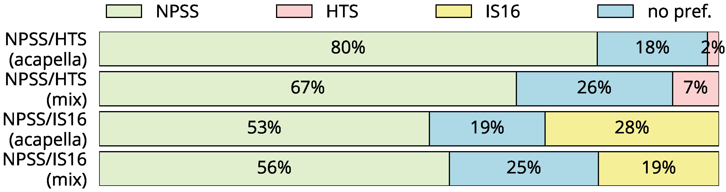
- Preference Test: For the systems trained on pseudo singing, we conducted an AB preference test. The 18 participants were asked for their preference between two different stimuli, or indicate no preference. The stimuli consisted of two short excerpts (<10 s) of one song per voice/language. Versions with and without background music were presented. We perform pairwise comparisons between our system and two other systems, resulting in a total of 24 stimuli.
5. Results
5.1. Quantitative Results
5.2. Qualitative Results
6. Conclusions
Acknowledgments
Author Contributions
Conflicts of Interest
Appendix A. Details Constrained Gaussian Mixture
Appendix B. Details Tuning Postprocessing
Appendix C. Model Hyperparameters

| Hyperparameter | Timbre Model | Pitch Model | ||
|---|---|---|---|---|
| Harmonic | Aperiodic | V/UV | F0 | |
| Feature dimensionality | 60 | 4 | 1 | 1 |
| Additional inputs (dim.) | - | harmonic (60) | harmonic (60) | - |
| aperiodic (4) | ||||
| Control inputs | prev. phn. class (one-hot) | |||
| cur. phn. class (one-hot) | ||||
| next phn. class (one-hot) | ||||
| prev. phn. identity (one-hot) | pos.-in-phn. (coarse) | |||
| cur. phn. identity (one-hot) | prev. note pitch (one-hot) | |||
| next phn. identity (one-hot) | cur. note pitch (one-hot) | |||
| pos.-in-phn. (coarse) | next note pitch (one-hot) | |||
| F0 (coarse) | prev. note dur. (coarse) | |||
| cur. note dur. (coarse) | ||||
| next note dur. (coarse) | ||||
| pos.-in-note (coarse) | ||||
| Input noise level | 0.4 | 0.4 | 0.4 | 0.4 |
| Generation temperature | piecewise linear | 0.01 | - | 0.01 |
| (0,0.05; 3,0.05; | ||||
| 8,0.5; 60,0.5) | ||||
| Initial causal convolution | ||||
| Residual channels | 130 | 20 | 20 | 100 |
| Dilated convolutions | ||||
| Num. layers | 5 | 5 | 5 | 13 |
| Num. layers per stage | 3 | 3 | 3 | 7 |
| Dilation factors | 1, 2, 4, 1, 2 | 1, 2, 4, 1, 2 | 1, 2, 4, 1, 2 | 1, 2, 4, 8, 16, 32, 64, |
| 1, 2, 4, 8, 16, 32 | ||||
| Receptive field (ms) | 100 | 100 | 100 | 1050 |
| Skip channels | 240 | 16 | 4 | 100 |
| Output stage | tanh → | tanh → | tanh → | tanh → |
| → CGM | → CGM | → sigmoid | → CGM | |
| Batch size | 32 | 32 | 32 | 64 |
| Num. valid out timesteps | 210 | 210 | 210 | 105 |
| Learning rate | 5 × 10⁻⁴, | 5 × 10⁻⁴, | 5 × 10⁻⁴, | 1 × 10⁻³, |
| (initial, decay, interval) | 1 × 10⁻⁵, 1 | 1 × 10⁻⁵, 1 | 1 × 10⁻⁵, 1 | - |
| Num. epochs (updates) | 1650 (82,500) | 1650 (82,500) | 1650 (82,500) | 235 (11,750) |
| Hyperparameter | Note Timing | Phoneme Duration |
|---|---|---|
| Input features | note duration (one-hot) | phoneme identity (one-hot) |
| prev. note duration (one-hot) | phoneme class (one-hot) | |
| 1st phoneme class (one-hot) | phoneme is vowel | |
| note position in bar (normalized) | phoneme kind (onset/nucleus/coda/inner) | |
| note is rest | note duration (one-hot) | |
| num. coda consonants prev. note | prev. note duration (one-hot) | |
| prev. note is rest | next note duration (one-hot) | |
| Target range (frames) | [−15,14], [−30,29] for rests | [5, 538] |
| Target discretization | 30 bins, linear | 50 bins, log scale |
| Architecture | input → dropout (0.81) → ReLU → dropout (0.9) → ReLU → dropout (0.9) → ReLU → dropout (0.81) → 30-way softmax | input → dropout (0.8) → gated tanh → dropout (0.8) (dilation = 2) → gated tanh → dropout (0.8) → gated tanh → dropout (0.64) → 50-way softmax |
| Batch size | 32 | 16 |
| Learning rate | 2 × 10⁻⁴ | 2 × 10⁻⁴ |
| Number of epochs | 140 | 210 |
References
- Bonada, J.; Umbert, M.; Blaauw, M. Expressive singing synthesis based on unit selection for the singing synthesis challenge 2016. In Proceedings of the 17th Annual Conference of the International Speech Communication Association (Interspeech), San Francisco, CA, USA, 8–12 September 2016; pp. 1230–1234. [Google Scholar]
- Bonada, J.; Serra, X. Synthesis of the Singing Voice by Performance Sampling and Spectral Models. IEEE Signal Process. Mag. 2007, 24, 67–79. [Google Scholar] [CrossRef]
- Saino, K.; Zen, H.; Nankaku, Y.; Lee, A.; Tokuda, K. An HMM-based singing voice synthesis system. In Proceedings of the 9th International Conference on Spoken Language Processing (ICSLP—Interspeech), Pittsburgh, PA, USA, 17–21 September 2006; pp. 2274–2277. [Google Scholar]
- Oura, K.; Mase, A.; Yamada, T.; Muto, S.; Nankaku, Y.; Tokuda, K. Recent development of the HMM-based singing voice synthesis system—Sinsy. In Proceedings of the 7th ISCA Workshop on Speech Synthesis (SSW7), Kyoto, Japan, 22–24 September 2010; pp. 211–216. [Google Scholar]
- Van den Oord, A.; Dieleman, S.; Zen, H.; Simonyan, K.; Vinyals, O.; Graves, A.; Kalchbrenner, N.; Senior, A.W.; Kavukcuoglu, K. WaveNet: A generative model for raw audio. CoRR arXiv 2016, arXiv:1609.03499. [Google Scholar]
- Blaauw, M.; Bonada, J. A neural parametric singing synthesizer. In Proceedings of the 18th Annual Conference of the International Speech Communication Association (Interspeech), Stockholm, Sweden, 20–24 August 2017; pp. 1230–1234. [Google Scholar]
- Yu, F.; Koltun, V. Multi-Scale Context Aggregation by Dilated Convolutions. In Proceedings of the 4th International Conference on Learning Representations (ICLR), San Juan, Puerto Rico, 2–4 May 2016. [Google Scholar]
- He, K.; Zhang, X.; Ren, S.; Sun, J. Deep residual learning for image recognition. In Proceedings of the 34th IEEE Conference on Computer Vision and Pattern Recognition (CVPR), Las Vegas, NV, USA, 27–30 June 2016; pp. 770–778. [Google Scholar]
- Reed, S.; van den Oord, A.; Kalchbrenner, N.; Bapst, V.; Botvinick, M.; de Freitas, N. Generating Interpretable Images with Controllable Structure; Technical Report; Google DeepMind: London, UK, 2016. [Google Scholar]
- Van den Oord, A.; Kalchbrenner, N.; Vinyals, O.; Espeholt, L.; Graves, A.; Kavukcuoglu, K. Conditional image generation with PixelCNN decoders. In Proceedings of the Advances in Neural Information Processing Systems 29 (NIPS), Barcelona, Spain, 5–10 December 2016; pp. 4790–4798. [Google Scholar]
- Van den Oord, A.; Kalchbrenner, N.; Kavukcuoglu, K. Pixel recurrent neural networks. In Proceedings of the 33rd International Conference on Machine Learning (ICML), New York, NY, USA, 19–24 June 2016; Volume 48, pp. 1747–1756. [Google Scholar]
- Salimans, T.; Karpathy, A.; Chen, X.; Kingma, D.P. PixelCNN++: Improving the PixelCNN with discretized logistic mixture likelihood and other modifications. In Proceedings of the 5th International Conference on Learning Representations (ICLR), Toulon, France, 24–26 April 2017. [Google Scholar]
- Blaauw, M.; Bonada, J. A Singing Synthesizer Based on PixelCNN. Presented at the María de Maeztu Seminar on Music Knowledge Extraction Using Machine Learning (Collocated with NIPS). Available online: http://www.dtic.upf.edu/~mblaauw/MdM_NIPS_seminar/ (accessed on 1 October 2017).
- Ranzato, M.; Chopra, S.; Auli, M.; Zaremba, W. Sequence level training with recurrent neural networks. In Proceedings of the 4th International Conference on Learning Representations (ICLR), San Juan, Puerto Rico, 2–4 May 2016. [Google Scholar]
- Wang, X.; Takaki, S.; Yamagishi, J. A RNN-based quantized F0 model with multi-tier feedback links for text-to-speech synthesis. In Proceedings of the 18th Annual Conference of the International Speech Communication Association (Interspeech), Stockholm, Sweden, 20–24 August 2017; pp. 1059–1063. [Google Scholar]
- Taylor, P. Text-to-Speech Synthesis; Cambridge University Press: Cambridge, UK, 2009; Chapter 9.1.4; p. 229. [Google Scholar]
- Umbert, M.; Bonada, J.; Blaauw, M. Generating singing voice expression contours based on unit selection. In Proceedings of the 4th Stockholm Music Acoustics Conference (SMAC), Stockholm, Sweden, 30 July–3 August 2013; pp. 315–320. [Google Scholar]
- Mase, A.; Oura, K.; Nankaku, Y.; Tokuda, K. HMM-based singing voice synthesis system using pitch-shifted pseudo training data. In Proceedings of the 11th Annual Conference of the International Speech Communication Association (Interspeech), Makuhari, Chiba, Japan, 26–30 September 2010; pp. 845–848. [Google Scholar]
- Nakamura, K.; Oura, K.; Nankaku, Y.; Tokuda, K. HMM-based singing voice synthesis and its application to Japanese and English. In Proceedings of the 39th IEEE International Conference on Acoustics, Speech and Signal Processing (ICASSP), Florence, Italy, 4–9 May 2014; pp. 265–269. [Google Scholar]
- Arik, S.Ö.; Diamos, G.; Gibiansky, A.; Miller, J.; Peng, K.; Ping, W.; Raiman, J.; Zhou, Y. Deep voice 2: Multi-speaker neural text-to-speech. In Proceedings of the Advances in Neural Information Processing Systems 30 (NIPS), Long Beach, CA, USA, 4–9 December 2017. [Google Scholar]
- Morise, M.; Yokomori, F.; Ozawa, K. WORLD: A vocoder-based high-quality speech synthesis system for real-time applications. IEICE Trans. Inf. Syst. 2016, 99, 1877–1884. [Google Scholar] [CrossRef]
- Morise, M. D4C, a band-aperiodicity estimator for high-quality speech synthesis. Speech Commun. 2016, 84, 57–65. [Google Scholar] [CrossRef]
- Tokuda, K.; Kobayashi, T.; Masuko, T.; Imai, S. Mel-generalized cepstral analysis—A unified approach to speech spectral estimation. In Proceedings of the 3rd International Conference on Spoken Language Processing (ICSLP), Yokohama, Japan, 18–22 September 1994. [Google Scholar]
- Ueda, N.; Nakano, R. Deterministic annealing EM algorithm. Neural Netw. 1998, 11, 271–282. [Google Scholar] [CrossRef]
- Ramachandran, P.; Paine, T.L.; Khorrami, P.; Babaeizadeh, M.; Chang, S.; Zhang, Y.; Hasegawa-Johnson, M.; Campbell, R.; Huang, T. Fast generation for convolutional autoregressive models. In Proceedings of the 5th International Conference on Learning Representations (ICLR), Toulon, France, 24–26 April 2017. [Google Scholar]
- Arik, S.Ö.; Chrzanowski, M.; Coates, A.; Diamos, G.; Gibiansky, A.; Kang, Y.; Li, X.; Miller, J.; Raiman, J.; Sengupta, S.; et al. Deep voice: Real-time neural text-to-speech. In Proceedings of the 34th International Conference on Machine Learning (ICML), Stockholm, Sweden, 10–15 July 2017; pp. 195–204. [Google Scholar]
- Kalchbrenner, N.; van den Oord, A.; Simonyan, K.; Danihelka, I.; Vinyals, O.; Graves, A.; Kavukcuoglu, K. Video pixel networks. CoRR arXiv 2016, arXiv:1610.00527. [Google Scholar]
- Kalchbrenner, N.; Espeholt, L.; Simonyan, K.; van den Oord, A.; Graves, A.; Kavukcuoglu, K. Neural machine translation in linear time. CoRR arXiv 2016, arXiv:1610.10099. [Google Scholar]
- Mehri, S.; Kumar, K.; Gulrajani, I.; Kumar, R.; Jain, S.; Sotelo, J.; Courville, A.C.; Bengio, Y. SampleRNN: An unconditional end-to-end neural audio generation model. In Proceedings of the 5th International Conference on Learning Representations (ICLR), Toulon, France, 24–26 April 2017. [Google Scholar]
- Sotelo, J.; Mehri, S.; Kumar, K.; Santos, J.F.; Kastner, K.; Courville, A.; Bengio, Y. Char2Wav: End-to-End speech synthesis. In Proceedings of the 5th International Conference on Learning Representations (ICLR), Toulon, France, 24–26 April 2017. [Google Scholar]
- Wang, Y.; Skerry-Ryan, R.J.; Stanton, D.; Wu, Y.; Weiss, R.J.; Jaitly, N.; Yang, Z.; Xiao, Y.; Chen, Z.; Bengio, S.; et al. Tacotron: A fully end-to-end text-to-speech synthesis model. In Proceedings of the 18th Annual Conference of the International Speech Communication Association (Interspeech), Stockholm, Sweden, 20–24 August 2017; pp. 4006–4010. [Google Scholar]
- Zen, H.; Senior, A. Deep mixture density networks for acoustic modeling in statistical parametric speech synthesis. In Proceedings of the 39th IEEE International Conference on Acoustics, Speech, and Signal Processing (ICASSP), Florence, Italy, 4–9 May 2014; pp. 3872–3876. [Google Scholar]
- Zen, H.; Sak, H. Unidirectional long short-term memory recurrent neural network with recurrent output layer for low-latency speech synthesis. In Proceedings of the 40th IEEE International Conference on Acoustics, Speech, and Signal Processing (ICASSP), South Brisbane, QLD, Australia, 19–24 April 2015; pp. 4470–4474. [Google Scholar]
- Tokuda, K.; Yoshimura, T.; Masuko, T.; Kobayashi, T.; Kitamura, T. Speech parameter generation algorithms for HMM-based speech synthesis. In Proceedings of the 25th IEEE International Conference on Acoustics, Speech, and Signal Processing (ICASSP), Istanbul, Turkey, 5–9 June 2000; Volume 3, pp. 1315–1318. [Google Scholar]
- Oura, K.; Mase, A.; Nankaku, Y.; Tokuda, K. Pitch adaptive training for HMM-based singing voice synthesis. In Proceedings of the 37th IEEE International Conference on Acoustics, Speech and Signal Processing (ICASSP), Kyoto, Japan, 25–30 March 2012; pp. 5377–5380. [Google Scholar]
- Shirota, K.; Nakamura, K.; Hashimoto, K.; Oura, K.; Nankaku, Y.; Tokuda, K. Integration of speaker and pitch adaptive training for HMM-based singing voice synthesis. In Proceedings of the 39th IEEE International Conference on Acoustics, Speech and Signal Processing (ICASSP), Florence, Italy, 4–9 May 2014; pp. 2559–2563. [Google Scholar]
- Nishimura, M.; Hashimoto, K.; Oura, K.; Nankaku, Y.; Tokuda, K. Singing voice synthesis based on deep neural networks. In Proceedings of the 17th Annual Conference of the International Speech Communication Association (Interspeech), San Francisco, CA, USA, 8–12 September 2016; pp. 2478–2482. [Google Scholar]
- Zen, H.; Nose, T.; Yamagishi, J.; Sako, S.; Masuko, T.; Black, A.W.; Tokuda, K. The HMM-based speech synthesis system (HTS) version 2.0. In Proceedings of the 6th ISCA Workshop on Speech Synthesis (SSW6), Bonn, Germany, 22–24 August 2007; pp. 294–299. [Google Scholar]
- Iglewicz, B.; Hoaglin, D.C. How to Detect and Handle Outliers; ASQC Basic References in Quality Control; ASQC Quality Press: Milwaukee, WI, USA, 1993. [Google Scholar]
- Takamichi, S.; Toda, T.; Black, A.W.; Neubig, G.; Sakti, S.; Nakamura, S. Postfilters to modify the modulation spectrum for statistical parametric speech synthesis. IEEE/ACM Trans. Audio Speech Lang. Process. 2016, 24, 755–767. [Google Scholar] [CrossRef]
- Umbert, M.; Bonada, J.; Goto, M.; Nakano, T.; Sundberg, J. Expression control in singing voice synthesis: Features, approaches, evaluation, and challenges. IEEE Signal Process. Mag. 2015, 32, 55–73. [Google Scholar] [CrossRef]
- ITU-R Recommendation BS.1534-3. Method for the Subjective Assessment of Intermediate Quality Levels of Coding Systems; Technical Report; International Telecommunication Union: Geneva, Switzerland, 2015. [Google Scholar]
- Kingma, D.P.; Ba, J.L. Adam: A method for stochastic optimization. In Proceedings of the 3rd International Conference on Learning Representations (ICLR), San Diego, CA, USA, 7–9 May 2015. [Google Scholar]


| System | Harmonic | Aperiodic | V/UV | ||
|---|---|---|---|---|---|
| MCD (dB) | MS-LSD (<25 Hz/Full, dB) | BAPD (dB) | FPR (%) | FNR (%) | |
| IS16 | 6.94 | - | 3.84 | - | |
| Sinsy-HMM | 7.01 | 8.09/18.50 | 4.09 | 15.90 | 0.68 |
| Sinsy-DNN | 5.41 | 13.76/29.87 | 5.02 | 13.75 | 0.63 |
| NPSS | 5.54 | 7.60/11.65 | 3.44 | 16.32 | 0.64 |
| System | Note Onset Deviations | Note Offset Deviations | Consonant Durations | ||||||
|---|---|---|---|---|---|---|---|---|---|
| MAE | RMSE | r | MAE | RMSE | r | MAE | RMSE | r | |
| Sinsy-HMM | 7.107 | 9.027 | 0.379 | 13.800 | 17.755 | 0.699 | 4.022 | 5.262 | 0.589 |
| NPSS | 6.128 | 8.383 | 0.419 | 12.100 | 18.645 | 0.713 | 3.719 | 4.979 | 0.632 |
| System | MS-LSD (<25 Hz, dB) | RSME (Cents) | r |
|---|---|---|---|
| Sinsy-HMM | 5.052 | 81.795 | 0.977 |
| Sinsy-DNN | 2.858 | 83.706 | 0.976 |
| NPSS | 2.008 | 105.980 | 0.963 |
| Voice (Language) | System | Harmonic | Aperiodic | V/UV | ||
|---|---|---|---|---|---|---|
| MCD (dB) | MS-LSD (<25 Hz/Full, dB) | BAPD (dB) | FPR (%) | FNR (%) | ||
| M1 (Eng.) | HTS | 4.95 | 11.09/22.44 | 2.72 | 16.10 | 2.46 |
| NPSS | 5.14 | 7.79/8.18 | 2.44 | 11.22 | 2.65 | |
| F1 (Eng.) | HTS | 4.75 | 10.25/22.09 | 4.07 | 15.60 | 1.01 |
| NPSS | 4.95 | 5.68/9.04 | 3.83 | 15.79 | 0.56 | |
| F2 (Spa.) | HTS | 4.88 | 11.07/22.28 | 3.62 | 1.85 | 2.21 |
| NPSS | 5.27 | 8.02/6.59 | 3.38 | 1.40 | 3.20 | |
| System | Mean Opinion Score |
|---|---|
| Hidden reference | 4.76 ± 0.04 |
| IS16 | 2.36 ± 0.11 |
| Sinsy-HMM | 2.98 ± 0.10 |
| Sinsy-DNN | 2.77 ± 0.10 |
| NPSS | 3.43 ± 0.11 |
© 2017 by the authors. Licensee MDPI, Basel, Switzerland. This article is an open access article distributed under the terms and conditions of the Creative Commons Attribution (CC BY) license (http://creativecommons.org/licenses/by/4.0/).
Share and Cite
Blaauw, M.; Bonada, J. A Neural Parametric Singing Synthesizer Modeling Timbre and Expression from Natural Songs. Appl. Sci. 2017, 7, 1313. https://doi.org/10.3390/app7121313
Blaauw M, Bonada J. A Neural Parametric Singing Synthesizer Modeling Timbre and Expression from Natural Songs. Applied Sciences. 2017; 7(12):1313. https://doi.org/10.3390/app7121313
Chicago/Turabian StyleBlaauw, Merlijn, and Jordi Bonada. 2017. "A Neural Parametric Singing Synthesizer Modeling Timbre and Expression from Natural Songs" Applied Sciences 7, no. 12: 1313. https://doi.org/10.3390/app7121313
APA StyleBlaauw, M., & Bonada, J. (2017). A Neural Parametric Singing Synthesizer Modeling Timbre and Expression from Natural Songs. Applied Sciences, 7(12), 1313. https://doi.org/10.3390/app7121313