Nonlinear Integral Type Observer Design for State Estimation and Unknown Input Reconstruction

Abstract

This paper is concerned with model-based robust observer designs for state observation and its application for unknown input reconstruction. Firstly, a sliding mode observer (SMO), which provides exponential convergence of estimation error, is designed for a class of multivariable perturbed systems. Observer gain matrices subject to specific structures are going to be imposed such that the unknown perturbation will not affect estimate precision during the sliding modes; Secondly, to improve discontinuous control induced in the SMO as well as pursue asymptotic estimate precision, a proportional-integral type observer (PIO) is further developed. Both the design procedures of the SMO and PIO algorithms are characterized as feasibility issues of linear matrix inequality (LMI) and thus the computations of the control parameters can be efficiently solved. Compared with the SMO, it will be demonstrated that the PIO is capable of achieving better estimation precision as long as the unknown inputs are continuous. Finally, a servo-drive flexible robot arm is selected as an example to demonstrate the applications of the robust observer designs.

1. Introduction

Sliding Mode Control (SMC) is a well-known control theory owing to its outstanding robustness properties against to parametric uncertainties and external disturbances [1]. Sliding mode observer (SMO) is a high performance state estimator well suited for nonlinear uncertain systems [2,3] with only output information available.

Sliding mode observers (SMOs) have been successfully implemented in real control engineering for state estimations. In [4], SMOs are designed for flux estimation of induction motors. For motion control systems subject to nonlienar frictions, a SMO is applied to estimation friction state information for achieving friction compensation purpose [5]. To get better control performance, recently a SMO [6] and an extended type SMO [7] are employed to estimate unknown external disturbances as well as modeling uncertainties in finite time. Building on the work [8], a SMO is applied to control aero-elastic response of flapped wing for the suppression of external excitation [9]. For nominal systems, high gain observer is also a good candidate for state estimation. However as pointed out in [10], estimation performance will be degraded for systems in the presence of uncertainties and disturbances. Therefore, the use of SMO is capable of enhancing estimation precision.

For many different control problems, searching the solutions of constrained equations may not be an easy task. A better way is to replace these equations by inequalities and the design problem can then be effectively solved by using linear matrix inequalities (LMIs) [11,12]. In this decade, multi-object LMI techniques have been widely applied for the existence problem of robust continuous/discrete time observer designs [13,14]. For SMO design, the work [8] provides a standard method based on coordinate transformation. A necessary and sufficient condition is derived for the switching surface determination. The designs were further refined and solved by LMIs [15]. When applying the SMO presented in [16], the system input-out matrix must satisfy an algebra equality, which can be taken as a minimization issue and was recently resolved via LMIs [17].

In recent years, SMO design has been widely investigated not only for state estimation [18,19], but for recovery of uncertainties as well [20,21]. Building on the equivalent control in ideal sliding modes [1], the core concept of model-based unknown input/faults reconstructions in control systems is the generation of residual signals which act as indicators of external input. The idea behind the use of the observer for disturbance recovery is to estimate the outputs of the system from the measurements by using a class of SMO [20,21].

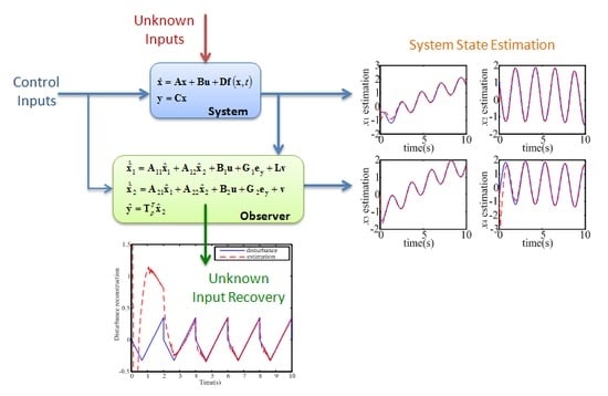
As a consequence, the first part of this paper concerns the structure of the SMO presented in [8,21] and the fault reconstruction ideas [20] to develop a SMO design for achieving state estimation as well as unknown input recovery. Existence of the SMO scheme is formulated in the form of LMIs such that all the observer gains involved in the SMO can be efficiently determined. However, estimate precision of SMO counts on the realization of infinite fast discontinuous control, which might be difficult to achieve ideally. Therefore, a second part of the work presents a proportional-integral type observer (PIO). The stability criterion of the PIO design is derived by the way of Lyapunov stability and the choice of observer gains applied in the PIO is resorted to solve a specific LMI. Inspired by and compare to the recent work [22], the proposed method is capable of reconstructing smooth as well as abrupt unknown inputs in an asymptotic level even though the L₂ condition is not satisfied.

Finally, simulations of a mechanical system subject to continuous and discontinuous unknown inputs are both addressed. Comparison studies are carried out and the estimation properties of the SMO and the PIO are also discussed.

2. Observer Design for Nonlinear Disturbed System

Consider the following nonlinear control system

$$\begin{array}{l}\dot{x}=Ax+Bu+Df\left(x,t\right)\\ y=Cx\end{array}$$

(1)

where the matrices $A\in {\mathfrak{R}}^{n\times n}$, $B\in {\mathfrak{R}}^{n\times m}$, $D\in {\mathfrak{R}}^{n\times q}$ and $C\in {\mathfrak{R}}^{p\times n}$ are known. The last term $f\left(x,t\right)$ is denoted as a lumped perturbation term containing system nonlinearities and unknown input signals. In this paper, we focus on the observer design for disturbance reconstruction as well as state estimation. Thus, system models are assumed to be known. In addition without loss of generality, the input/perturbation distribution matrices are of full rank. The following assumptions are imposed in this paper.

Assumption 1.

The matrices $C$ and $D$ satisfy that $rank\left(CD\right)=q$.

Assumption 2.

The system is observable and the dimensions $n>p\ge m$ and $p>q$ are considered.

Assumption 3.

The nonlinear term is bounded by a known constant $\delta$; that is $\Vert f\left(x,t\right)\Vert \le \delta$.

Applying a state transformation $x\to T_{o}x$ in which $T_o={\left[\begin{array}{cc}\mathcal{N}\left(C\right)& C^T\end{array}\right]}^T$ and $T_o^{-1}=\left[\begin{array}{cc}\mathcal{N}\left(C\right)& C^T{\left(C{C}^T\right)}^{-1}\end{array}\right]$, gives

$$\begin{array}{l}{\dot{x}}_1=A_{11}{x}_1+A_{12}{x}_2+B_{1}u+D_{1}f\left(x,t\right)\\ {\dot{x}}_2=A_{21}{x}_1+A_{22}{x}_2+B_{2}u+D_{2}f\left(x,t\right)\\ y=x_2\end{array}$$

(2)

where $\mathcal{N}(•)$ denotes as null space $D_1\in {\mathfrak{R}}^{\left(n-p\right)\times q}$ and $D_2\in {\mathfrak{R}}^{p\times q}$.

Based on Assumptions 1 and 2, apply a coordinate transformation matrix $T_D$ similar to [20] as follows

$$T_D=\left[\begin{array}{cc}{I}_{n-p}& -D_1{\left(D_2^T{D}_2\right)}^{-1}{D}_2^T\\ 0& T_p\end{array}\right]$$

(3)

where $T_p\in {\mathfrak{R}}^{p\times p}$ is an orthogonal matrix satisfying $T_p{D}_2=\left[\begin{array}{c}0\\ D_{222}\end{array}\right]\begin{array}{l}\updownarrow p-q\hfill \\ \updownarrow q\hfill \end{array}$.

Let $D_{22}=T_p{D}_2$ and then the system (2) in a new coordinate space can be further represented by

$$\begin{array}{l}{\dot{x}}_1=A_{11}{x}_1+A_{12}{x}_2+B_{1}u\\ {\dot{x}}_2=A_{21}{x}_1+A_{22}{x}_2+B_{2}u+D_{22}f\left(x,t\right)\\ y=\left[\begin{array}{cc}0& T_p^T\end{array}\right]x=T_p^T{x}_2\end{array}$$

(4)

where $A_{11}\in {\mathfrak{R}}^{\left(n-p\right)\times \left(n-p\right)}$, $A_{12}\in {\mathfrak{R}}^{\left(n-p\right)\times p}$, $A_{21}\in {\mathfrak{R}}^{p\times \left(n-p\right)}$, $A_{22}\in {\mathfrak{R}}^{p\times p}$, $B_1\in {\mathfrak{R}}^{\left(n-p\right)\times m}$ and $B_2\in {\mathfrak{R}}^{p\times m}$.

By using the coordinate transformations, the control systems are going to be represented by a canonical form and hence the robust SMO design can be easily carried out.

For system (4), firstly apply the following observer

$$\begin{array}{l}{\dot{\widehat{x}}}_1=A_{11}{\widehat{x}}_1+A_{12}{\widehat{x}}_2+B_{1}u+G_1{e}_y+Lv\\ {\dot{\widehat{x}}}_2=A_{21}{\widehat{x}}_1+A_{22}{\widehat{x}}_2+B_{2}u+G_2{e}_y+v\\ \widehat{y}=T_p^T{\widehat{x}}_2\end{array}$$

(5)

where $e_y=y-\widehat{y}=T_p^T\left(x_2-{\widehat{x}}_2\right)$. $G_1\in {\mathfrak{R}}^{\left(n-p\right)\times p}$, $G_2\in {\mathfrak{R}}^{p\times p}$ and $L\in {\mathfrak{R}}^{\left(n-p\right)\times p}$ are observer gain matrices and $v$ denotes as an observer control input. The SMO structure consists of switching terms added to a Luenberger observer [23].

From (2) and (5), it leads to the following error dynamics

$$\begin{array}{l}{\dot{e}}_1=A_{11}{e}_1+A_{12}{e}_2-G_1{e}_y-Lv\\ {\dot{e}}_2=A_{21}{e}_1+A_{22}{e}_2-G_2{e}_y-v+D_{22}f\left(x,t\right)\\ e_y=T_p^T{e}_2\end{array}$$

(6)

Equation (6) can be represented as the following compact form

$$\begin{array}{l}{\dot{e}}_1=A_{11}{e}_1+\left(A_{12}-G_1{T}_p^T\right)e_2-Lv\\ {\dot{e}}_2=A_{21}{e}_1+\left(A_{22}-G_2{T}_p^T\right)e_2-v+D_{22}f\left(x,t\right)\\ e_y=T_p^T{e}_2\end{array}$$

(7)

Since only $e_y$ is available, design of an output based sliding surface $S_o$ should depend on $e_y$ (or $e_2$) only. For example when $S_o=e_2$ is selected, by applying $v=\rho sign\left(S_o\right)$ in which $\rho >\Vert A_{21}{e}_1+D_{22}f\left(x,t\right)\Vert$, then $S_o={\dot{S}}_o=0$ is attained in finite time. Therefore $v$ is now replaced by the so-called equivalent control denoted by $v_{eq}$.

During the sliding motions, the equivalent control effort can be represented by

$$v_{eq}=A_{21}{e}_1+D_{22}f\left(x,t\right)$$

(8)

It is clear that the reconstruction of fault signals lies in the application of the equivalent output injection concept [8,15,18]. Therefore, it is necessary to maintain an ideal sliding motion.

On the other hand, the reduced order dynamics in the sliding mode is dominated by

$${\dot{e}}_1=\left(A_{11}-L{A}_{21}\right)e_1-L{D}_{22}f\left(x,t\right)$$

(9)

By using preceding coordinate transformation, it can be clearly observed from (9) that the pair $\left(A,C\right)$ is observable, it follows that the pair $\left(A_{11},A_{21}\right)$ is observable as well. Let ${\overline{A}}_{11}:=A_{11}-L{A}_{21}$, it is obviously that can be achieved by appropriate choices of $L$. Nevertheless, the reduced order dynamics is going to be perturbed by the perturbation term $f\left(x,t\right)$ through the observer gain matrix $L$. The asymptotic estimation level can be reached by applying $L=0$ as long as $\lambda \left(A_{11}\right)<0$ is naturally satisfied. Nevertheless, this achievement depends on the property of $A_{11}$, which may not always be the case. As a consequence, the following task is dedicated to design an appropriate control structure for (9) so that exponential estimation level could be obtained. If $e_1\to 0$ could be attained, it follows that $f\left(x,t\right)\to {\left(D_{22}^T{D}_{22}\right)}^{-1}{D}_{22}^T{v}_{eq}$.

To this aim, further apply a coordinate transformation to system (7) by $\overline{e}=T_{L}e$ in which

$$T_L=\left[\begin{array}{cc}{I}_{n-p}& -L\\ 0& I_p\end{array}\right] \& T_L^{-1}=\left[\begin{array}{cc}{I}_{n-p}& L\\ 0& I_p\end{array}\right]$$

(10)

Then, (7) can be represented by

$$\begin{array}{l}{\dot{\overline{e}}}_1={\overline{A}}_{11}{\overline{e}}_1+\left({\overline{A}}_{12}-{\overline{G}}_1{T}_p^T\right){\overline{e}}_2-L{D}_{22}f\left(x,t\right)\\ {\dot{\overline{e}}}_2={\overline{A}}_{21}{\overline{e}}_1+\left({\overline{A}}_{22}-{\overline{G}}_2{T}_p^T\right){\overline{e}}_2-v+D_{22}f\left(x,t\right)\\ {\overline{e}}_y=T_p^{-1}{\overline{e}}_2\end{array}$$

(11)

where the matrices are given by ${\overline{A}}_{11}=A_{11}-L{A}_{21}$, ${\overline{A}}_{12}=A_{12}-L{A}_{22}+A_{11}L-L{A}_{21}L$, ${\overline{A}}_{21}=A_{21}$, ${\overline{A}}_{22}=A_{21}L+A_{22}$, ${\overline{G}}_1=G_1-L{G}_2$ and ${\overline{G}}_2=G_2$.

Designing the following gain matrices

$$\{\begin{array}{l}{\overline{G}}_1={\overline{A}}_{12}{T}_p\\ {\overline{G}}_2=\left({\overline{A}}_{22}-{\overline{A}}_{22}^s\right)T_p\end{array}\iff \{\begin{array}{l}{G}_1={\overline{A}}_{12}{T}_p+L{G}_2\\ G_2=\left({\overline{A}}_{22}-{\overline{A}}_{22}^s\right)T_p\end{array}$$

(12)

and applying to (11) follows

$$\begin{array}{l}{\dot{\overline{e}}}_1={\overline{A}}_{11}{\overline{e}}_1-L{D}_{22}f\left(x,t\right)\\ {\dot{\overline{e}}}_2={\overline{A}}_{21}{\overline{e}}_1+{\overline{A}}_{22}^s{\overline{e}}_2-v+D_{22}f\left(x,t\right)\end{array}$$

(13)

where ${\overline{A}}_{22}^s$ is also a decision variable needs to be determined. Equation (13) shows that the estimation precision might be deteriorated by $f\left(x,t\right)$. Fortunately, owing to the property $p>q$, there exists a design degree of freedom on the selection of the gain matrix $L$ such that the error dynamics (9) is insensitive to $f\left(x,t\right)$. Therefore, the control object is to consider a structural constrain imposing on an observer gain matrices and solve them through LMIs.

By assigning the specific structure $L=\left[\begin{array}{cc}{L}_1& L_2\end{array}\right]=\left[\begin{array}{cc}{L}_1& 0\end{array}\right]$, where $L_1\in {\mathfrak{R}}^{\left(n-p\right)\times \left(p-q\right)}$ and $L_2\in 0^{\left(n-p\right)\times q}$, one can easily get

$$\{\begin{array}{l}{\overline{A}}_{11}=A_{11}-L{A}_{21}=A_{11}-\left[\begin{array}{cc}{L}_1& L_2\end{array}\right]\left[\begin{array}{c}{A}_{211}\\ A_{212}\end{array}\right]=A_{11}-L_1{A}_{211}\\ L{D}_{22}=L\left[\begin{array}{c}0\\ D_{222}\end{array}\right]=\left[\begin{array}{cc}{L}_1& L_2\end{array}\right]\left[\begin{array}{c}0\\ D_{222}\end{array}\right]=L_2{D}_{222}=0\end{array}$$

(14)

where $A_{211}\in {\mathfrak{R}}^{\left(p-q\right)\times \left(n-p\right)}$ and $A_{212}\in {\mathfrak{R}}^{q\times \left(n-p\right)}$.

Therefore, the design object turns into a feasibility problem on the selection of $L_1$ such that $\lambda \left({\overline{A}}_{11}\right)=\lambda \left(A_{11}-L_1{A}_{211}\right)<0$.

Based on (14), let $\mathcal{X}=\left[\begin{array}{c}{\overline{e}}_1\\ {\overline{e}}_2\end{array}\right]$ and $\mathbf{𝒶}\mathbf{𝒸}=\left[\begin{array}{cc}{\overline{A}}_{11}& 0\\ {\overline{A}}_{21}& {\overline{A}}_{22}^s\end{array}\right]$, consider a system partition

$$\mathbf{𝒶}\mathbf{𝒸}=\mathbf{𝒶}-\left({\mathcal{L}}_1\mathcal{C}+{\mathcal{L}}_2\right)$$

(15)

where the matrices are defined by

$$\{\begin{array}{l}\mathbf{𝒶}=\left[\begin{array}{cc}{A}_{11}& 0\\ {\overline{A}}_{21}& 0\end{array}\right],{\mathcal{L}}_1=\left[\begin{array}{ll}{L}_1\hfill & 0_{\left(n-p\right)\times \left(n-p+q\right)}\hfill \\ 0_{p\times \left(p-q\right)}\hfill & 0_{p\times \left(n-p+q\right)}\hfill \end{array}\right]\\ {\mathcal{L}}_2=\left[\begin{array}{ll}{0}_{\left(n-p\right)\times \left(n-p\right)}\hfill & 0_{\left(n-p\right)\times p}\hfill \\ 0_{p\times \left(n-p\right)}\hfill & -{\overline{A}}_{22}^s\hfill \end{array}\right],\mathcal{C}=\left[\begin{array}{ll}{A}_{211}\hfill & 0_{\left(p-q\right)\times p}\hfill \\ 0_{\left(n-p+q\right)\times \left(n-p\right)}\hfill & 0_{\left(n-p+q\right)\times p}\hfill \end{array}\right]\end{array}$$

(16)

Then system (13) turns into

$$\dot{\mathcal{X}}=\mathbf{𝒶}\mathbf{𝒸}\mathcal{X}+\left[\begin{array}{c}0\\ -v+D_{22}f\left(x,t\right)\end{array}\right]$$

(17)

Consider the linear part of (17) and a positive definite symmetric matrix $\mathcal{P}=diag\left(P_1,P_2\right)$, the nominal closed-loop dynamics is said to be quadratic stable if the inequality

$$\mathbf{𝒶}{\mathbf{𝒸}}^T\mathcal{P}+\mathcal{P}\mathbf{𝒶}\mathbf{𝒸}<0$$

(18)

is attained.

The left-hand-side of (18) can be rewritten in detail as follows

$$\left[\begin{array}{cc}{F}_1& F_3^T\\ F_3& F_2\end{array}\right]:=\left[\begin{array}{cc}{\left(A_{11}-L{A}_{21}\right)}^T{P}_1+P_1\left(A_{11}-L{A}_{21}\right)& A_{21}^T{P}_2\\ P_2{A}_{21}& {\overline{A}}_{22}^{sT}{P}_2+P_2{\overline{A}}_{22}^s\end{array}\right]$$

(19)

Consider Shur complement, the quadratic stability is achieved if and only if following inequalities are simultaneously guaranteed.

$$\begin{array}{r}{F}_1<0,F_2<0\\ F_1-F_3^T{F}_2^{-1}{F}_3<0\end{array}$$

(20)

It can be easily found that to achieve the quadratic stability, one has to firstly determine $L$ and ${\overline{A}}_{22}^{sT}$ to satisfy $F_1<0$ and $F_2<0$. In addition, one must finally check whether $F_1-F_3^T{F}_2^{-1}{F}_3<0$ is also guaranteed. Therefore, it leads to a two steps design. The following is going to propose a convenient way to resolve the preceding issues simultaneously via a LMI design, where the specific structure of $L$ needs to be considered.

Proposition 1.

For the observer error dynamics (17), by applying the following sliding controller

$$\{\begin{array}{l}v=\rho \left(x,t\right)\frac{P_{2}s}{\Vert P_{2}s\Vert }\\ S_o=\left\{{\overline{e}}_y=e_y\in {\mathfrak{R}}^p|s=T_p{\overline{e}}_y={\overline{e}}_2=e_2=0\right\}\end{array}$$

(21)

and

$$\rho \left(x,t\right)\ge \delta \Vert D_{22}\Vert +\eta$$

(22)

where $\eta >0$ is a given value, then the prescribed sliding motions are eventually fulfilled as long as the following inequality is feasible

$${\mathbf{𝒶}}^T\mathcal{P}+\mathcal{P}\mathbf{𝒶}-{\mathcal{C}}^T{\mathcal{K}}_1^T-{\mathcal{K}}_1\mathcal{C}-{\mathcal{K}}_2^T-{\mathcal{K}}_2+2\alpha \mathcal{P}<0$$

(23)

where ${\mathcal{K}}_1={\mathcal{PL}}_1$ and ${\mathcal{K}}_2={\mathcal{PL}}_2$ are both control variables requiring to be determined.

Moreover, the high gain feedback is avoidable by further considering the following minimization process:

$$min \ell subject to \left[\begin{array}{ccc}-\ell & {\mathcal{K}}_1^T& {\mathcal{K}}_2^T\\ {\mathcal{K}}_1& -\ell & 0\\ {\mathcal{K}}_2& 0& -\ell \end{array}\right]<0 and \mathcal{P}>I$$

(24)

The matrices applied in (21)–(24) are going to be addressed in the following proof.

Proof of the quadratic stability.

Select as a Lyapunov function $\mathrm{V}={\mathrm{X}}^T\mathrm{PX}$ in which $\mathcal{P}={\mathcal{P}}^T=\left[\begin{array}{cc}{P}_1& 0\\ 0& P_2\end{array}\right]>0$. Taking the time derivative leads to

$$\begin{array}{ll}\dot{\mathcal{V}}& ={\mathcal{X}}^T(\mathbf{𝒶}{\mathbf{𝒸}}^T\mathcal{P}+\mathcal{P}\mathbf{𝒶}\mathbf{𝒸})\mathcal{X}+2{\overline{e}}_2^T{P}_2(-v+D_{22}f(x,t))\\ & ={\mathcal{X}}^T({\mathbf{𝒶}}^T\mathcal{P}+\mathcal{P}\mathbf{𝒶}-{({\mathcal{L}}_1\mathcal{C}+{\mathcal{L}}_2)}^T\mathcal{P}-\mathcal{P}({\mathcal{L}}_1\mathcal{C}+{\mathcal{L}}_2))\mathcal{X}\\ & +2{\overline{e}}_2^T{P}_2(-v+D_{22}f(x,t))\\ & \le {\mathcal{X}}^T\mathcal{MX}-2{\overline{e}}_2^T{P}_2\left(\rho (x,t)\frac{P_{2}s}{\Vert P_{2}s\Vert }-\Vert D_{22}f(x,t)\Vert \right)\\ & \le {\mathcal{X}}^T\mathcal{MX}-2\Vert P_{2}s\Vert (\rho (x,t)-\delta \Vert D_{22}\Vert )\\ & \le {\mathcal{X}}^T\mathcal{MX}-2\eta \Vert P_{2}s\Vert \end{array}$$

(25)

where $\mathcal{M}={\mathbf{𝒶}}^T\mathcal{P}+\mathcal{P}\mathbf{𝒶}-{\left({\mathcal{L}}_1\mathcal{C}+{\mathcal{L}}_2\right)}^T\mathcal{P}-\mathcal{P}\left({\mathcal{L}}_1\mathcal{C}+{\mathcal{L}}_2\right)$. As a consequence, the quadratic stability is available if $\mathcal{M}<0$ is fulfilled. The design object can be achieved if the following inequality holds

$${\mathbf{𝒶}}^T\mathcal{P}+\mathcal{P}\mathbf{𝒶}-{\left({\mathcal{L}}_1\mathcal{C}+{\mathcal{L}}_2\right)}^T\mathcal{P}-\mathcal{P}\left({\mathcal{L}}_1\mathcal{C}+{\mathcal{L}}_2\right)<-2\alpha \mathcal{P}$$

(26)

where $\alpha$ provides a guaranteed convergence speed of observer error. Providing (26) is feasible, the exponential stability with a prescribed decay speed is guaranteed; that is $\dot{\mathcal{V}}\le -2\alpha \mathcal{V}$.

Based on the definition ${\mathcal{K}}_1={\mathcal{PL}}_1$ and ${\mathcal{K}}_2={\mathcal{PL}}_2$, (26) is equivalent to

$${\mathbf{𝒶}}^T\mathcal{P}+\mathcal{P}\mathbf{𝒶}-{\mathcal{C}}^T{\mathcal{K}}_1^T-{\mathcal{K}}_1\mathcal{C}-{\mathcal{K}}_2^T-{\mathcal{K}}_2+2\alpha \mathcal{P}<0$$

(27)

Due to the structure of the observer gain, the auxiliary control variables ${\mathcal{K}}_1$ and ${\mathcal{K}}_2$ are respectively imposed to be with the following specific configuration

$$\begin{array}{l}{\mathcal{K}}_1=\left[\begin{array}{ll}{\ast }_{\left(n-p\right)\times \left(p-q\right)}\hfill & 0_{\left(n-p\right)\times \left(n-p+q\right)}\hfill \\ 0_{p\times \left(p-q\right)}\hfill & 0_{p\times \left(n-p+q\right)}\hfill \end{array}\right]\\ {\mathcal{K}}_2=\left[\begin{array}{ll}{0}_{\left(n-p\right)\times \left(n-p\right)}\hfill & 0_{\left(n-p\right)\times p}\hfill \\ 0_{p\times \left(n-p\right)}\hfill & {\ast }_{p\times p}\hfill \end{array}\right]\end{array}$$

(28)

where the symbol “*” stands for undetermined nonzero sub-matrices and the solutions are going to be carried out via LMI solver.

To avoid high gain feedback, let $\mathcal{K}=\left[\begin{array}{c}{\mathcal{K}}_1\\ {\mathcal{K}}_2\end{array}\right]$ and consider $\Vert \mathcal{K}\Vert <\ell$, where $\ell$ is going to be minimized. The minimization problem can be characterized as the following LMI:

$$\min \ell \mathrm{subject} \mathrm{to} \left[\begin{array}{ccc}-\ell & {\mathcal{K}}_1^T& {\mathcal{K}}_2^T\\ {\mathcal{K}}_1& -\ell & 0\\ {\mathcal{K}}_2& 0& -\ell \end{array}\right]<0\text{ and }\mathcal{P}>1$$

(29)

Note that provided (27) and (29) are feasible, it can be concluded that the inequalities

$$\begin{array}{r}{\overline{A}}_{11}{P}_1+P_1{\overline{A}}_{11}<-2\alpha P_1\\ {\overline{A}}_{22}^{sT}{P}_2+P_2{\overline{A}}_{22}^s<-2\alpha P_2\end{array}$$

(30)

are guaranteed as well. ☐

Proof of the existence of sliding motions.

For sliding dynamics, apply a Lyapunov function as follows

$$V_s=s^T{P}_{2}s$$

(31)

Based on (30), taking the time derivative of (31) gives

$$\begin{array}{l}{\dot{V}}_s=s^T\left({\overline{A}}_{22}^{sT}{P}_2+P_2{\overline{A}}_{22}^s\right)s\\ +2s^T\left(P_2{\overline{A}}_{21}{e}_1-P_{2}v+P_2{D}_{22}f\left(x,t\right)\right)\\ \le -2\alpha s^T{P}_{2}s+2s^T\left(P_2{\overline{A}}_{21}{e}_1-P_{2}v+P_2{D}_{22}f\left(x,t\right)\right)\\ \le -2\alpha s^T{P}_{2}s-2\Vert P_{2}s\Vert \left(\eta -\Vert {\overline{A}}_{21}{e}_1\Vert \right)\end{array}$$

(32)

Since only system outputs are available, the norm bound $\Vert {\overline{A}}_{21}{e}_1\Vert$ is not available. Therefore, prescribed sliding motions might not be attained immediately for an arbitrary given $\eta$. It is well known that a large value of $\eta$ is capable of realizing approaching phase immediately but unavoidably brings about serious control chattering. Examine again the Lyapunov function presented in (25). Owing to the properties of the quadratic stability, the observer system trajectories will eventually enter the sliding domain and therefore the prescribed sliding modes can be fulfilled in finite time. In other words, there must exist positive constants $\varphi$ and ${\varphi }^{\ast }$ such that the condition $\varphi \ge \eta -\Vert {\overline{A}}_{21}{e}_1\Vert \ge {\varphi }^{\ast }>0$ could be eventually satisfied. Under this circumstance, (32) reduces to

$$\begin{array}{ll}{\dot{V}}_s& \le -2\alpha s^T{P}_{2}s-2{\varphi }^{\ast }\Vert P_{2}s\Vert \\ & \le -2\alpha V_s-2{\varphi }^{\ast }{\lambda }_{\min }^{1/2}\left(P_2\right)\sqrt{V_s}\end{array}$$

(33)

where ${\Vert P_{2}s\Vert }^2={\left(P_2^{1/2}s\right)}^{T}P\left(P_2^{1/2}s\right)\ge {\lambda }_{\min }\left(P_2\right){\Vert P_2^{1/2}s\Vert }^2={\lambda }_{\min }\left(P_2\right)V_s$ is utilized in (33).

Equation (33) shows that the system trajectories hit the sliding manifold in finite time $t_r$ described as follows

$$t_r=t_p+\frac{1}{\alpha }\cdot \ln \left(\frac{\alpha }{{\varphi }^{\ast }{\lambda }_{\min }^{1/2}\left(P_2\right)}{V}_s{\left(t_p\right)}^{1/2}+1\right)$$

(34)

where $t_p$ stands for a time instant in which the approaching condition is attained. ☐

Remark 1.

The requirements of quadratic stability and fulfillment of sliding motions can be formulated as a feasibility problem of a single LMI subject to a specific matrix configuration. By using the preceding LMIs (23) and (24), the gain pair $\left(L_1,{\overline{A}}_{22}^s\right)$ can be simultaneously determined without inducing high gain phenomenon and the resulting observer error dynamics is with a guaranteed convergence speed.

3. Robust Proportional-Integral Type Observer Design

In the preceding section, a sliding observer with systematic control gain generation is developed. However, the robustness of the SMO relies on the realization of infinite fast control switching and thereby estimate precision depends on computation speed. It has been pointed out that in the ideal sliding motions, the discontinuous control stands for the necessary input effort to main the systems in sliding modes and compensate unknown perturbations [20]. Therefore, the external unknown signals should be recovered by filtering the control signals or by using boundary layer techniques. However, the estimation precision will be unavoidable deteriorated. To avoid the discontinuous control effort applied in observer and simultaneously reconstruct external unknown inputs, the following work is to inherit the previous SMO design framework and integrate the ideas presented in [24,25] for smooth multivariable robust observer design.

Referring to (12), the pair $\left({\overline{G}}_1,{\overline{G}}_2\right)$ is now designed by

$$\{\begin{array}{l}{\overline{G}}_1={\overline{A}}_{12}{T}_p\\ {\overline{G}}_2={\overline{A}}_{22}{T}_p\end{array}$$

(35)

Considering (14) together with (35), one can represent the observer error dynamics (13) by

$$\begin{array}{l}{\dot{\overline{e}}}_1={\overline{A}}_{11}{\overline{e}}_1\\ {\dot{\overline{e}}}_2={\overline{A}}_{21}{\overline{e}}_1-v+D_{22}f\left(x,t\right)\end{array}$$

(36)

where ${\overline{A}}_{11}$ is already Hurwitz.

Proposition 2.

Suppose that there exists a known function $\zeta \left(t\right)$ such that $\Vert \dot{f}\left(x,t\right)\Vert \le \zeta \left(t\right)$ for $\forall t$. For the transformed system (36), the estimation error dynamics is asymptotic stable by applying the following proportional-integral control

$$v=K_P{\overline{e}}_2+{\displaystyle {\int }_0^t\left(K_I{\overline{e}}_2+\mathsf{\xi }\mathrm{sgn}\left({\overline{e}}_2\right)\right)d\tau }$$

(37)

where $K_P\in {\mathfrak{R}}^{p\times p}$, $K_I\in {\mathfrak{R}}^{p\times p}$, $\mathsf{\xi }=diag\left({\xi }_i\right)$ and $\mathrm{sgn}\left({\overline{e}}_2\right)=sign\left({\overline{e}}_{2i}\right)$ with $i=1\cdots p$.

The control gains applied in (37) satisfy

$$\begin{array}{l}\overline{\mathcal{P}}{\mathcal{A}}^T+\mathcal{A}\overline{\mathcal{P}}-{\mathcal{L}}^T{\mathcal{B}}^T-\mathcal{B}\mathcal{L}+2\beta \overline{\mathcal{P}}<0\\ \mathsf{\xi }>\zeta \left(t\right)\end{array}$$

(38)

where $\beta >0$, $\overline{\mathcal{P}}={\mathcal{P}}^{-1}$, $\mathcal{P}={\mathcal{P}}^T>0$, $\mathcal{L}=\mathcal{K}\overline{\mathcal{P}}$, and the matrices are with the following specific structures

$$\begin{array}{l}\mathcal{A}=\left[\begin{array}{ccc}{\overline{A}}_{11}& 0& 0\\ 0& 0& I_p\\ {\overline{A}}_{21}{\overline{A}}_{11}& 0& 0\end{array}\right]\in {\mathfrak{R}}^{\left(n+p\right)\times \left(n+p\right)}\\ \mathcal{B}=\left[\begin{array}{c}0\\ 0\\ I_p\end{array}\right]\in {\mathfrak{R}}^{\left(n+p\right)\times p},\mathcal{K}=\left[\begin{array}{ccc}0& K_I& K_P\end{array}\right]\end{array}$$

(39)

and

$$\mathcal{P}=\left[\begin{array}{cc}{\mathcal{P}}_1& 0\\ 0& {\mathcal{P}}_2\end{array}\right]\begin{array}{l}\updownarrow n-p\hfill \\ \updownarrow 2p\hfill \end{array},{\mathcal{P}}_2=\left[\begin{array}{cc}{\mathcal{P}}_{21}& {\mathcal{P}}_{23}\\ {\mathcal{P}}_{23}& {\mathcal{P}}_{22}\end{array}\right]\begin{array}{l}\updownarrow p\hfill \\ \updownarrow p\hfill \end{array}$$

(40)

Note that ${\mathcal{P}}_{23}$ is non-negative diagonal matrix.

Proof. 

Substituting (37) into (36) yields

$$\begin{array}{l}{\dot{\overline{e}}}_1={\overline{A}}_{11}{\overline{e}}_1\\ {\dot{\overline{e}}}_2={\overline{A}}_{21}{\overline{e}}_1-K_P{\overline{e}}_2-{\displaystyle {\int }_0^t\left(K_I{\overline{e}}_2+\mathsf{\xi }\mathrm{sgn}\left({\overline{e}}_2\right)\right)d\tau }+D_{22}f\left(x,t\right)\end{array}$$

(41)

To address the stability of the observer error dynamics, let ${\dot{\overline{e}}}_2={\overline{e}}_3$ and then (41) can be represented by an augmented system described as follows

$$\begin{array}{l}{\dot{\overline{e}}}_1={\overline{A}}_{11}{\overline{e}}_1\\ {\dot{\overline{e}}}_2={\overline{e}}_3\\ {\dot{\overline{e}}}_3={\overline{A}}_{21}{\overline{A}}_{11}{\overline{e}}_1-K_P{\overline{e}}_3-K_I{\overline{e}}_2-\xi \mathrm{sgn}\left({\overline{e}}_2\right)+D_{22}\dot{f}\left(x,t\right)\end{array}$$

(42)

Define an augmented state variable by $\mathbf{𝓍}=col\left({\overline{e}}_1,{\overline{e}}_2,{\overline{e}}_3\right)$ and represent (42) in the compact form

$$\dot{\mathbf{𝓍}}={\mathcal{A}}_{\mathcal{C}}\mathbf{𝓍}+\mathcal{B}\left(-\mathsf{\xi }\mathrm{sgn}\left({\overline{e}}_2\right)+D_{22}\dot{f}\left(x,t\right)\right)$$

(43)

in which

$${\mathcal{A}}_{\mathcal{C}}=\left[\begin{array}{ccc}{\overline{A}}_{11}& 0& 0\\ 0& 0& I_p\\ {\overline{A}}_{21}{\overline{A}}_{11}& -K_I& -K_P\end{array}\right]\in {\mathfrak{R}}^{\left(n+p\right)\times \left(n+p\right)}$$

(44)

Note that the extended system (43) is only used for stability analysis and control gain determination purposes. No extra state information needs to be involved for the observer implementation.

By applying $\mathsf{\xi }>\zeta \left(t\right)$, the closed-loop observer dynamics can be governed by the following auxiliary system

$$\dot{\mathbf{𝓍}}={\mathcal{A}}_{\mathcal{C}}\mathbf{𝓍}+\mathcal{B}\left(-\tilde{\mathsf{\xi }}\mathrm{sgn}\left({\overline{e}}_2\right)\right)$$

(45)

where $\tilde{\mathsf{\xi }}=diag\left({\tilde{\xi }}_i\right)$, ${\tilde{\xi }}_i\in \left[{\tilde{\xi }}_i^{+},{\tilde{\xi }}_i^{-}\right]$, ${\tilde{\xi }}_i^{+}=\Vert \mathsf{\xi }\Vert +\max \left(\zeta \left(t\right)\right)>0$ and ${\tilde{\xi }}_i^{-}=\Vert \mathsf{\xi }\Vert -\max \left(\zeta \left(t\right)\right)>0$.

For (45), the following Lyapunov candidate is proposed

$$\mathcal{V}={\mathbf{𝓍}}^T\mathcal{P}\mathbf{𝓍}+2{\displaystyle {\sum }_{i=1}^p{\mathcal{P}}_{22}^i{\tilde{\xi }}_i\left|{\overline{e}}_2^i\right|}$$

(46)

where ${\mathcal{P}}_{22}^i$ and ${\overline{e}}_2^i$ stands for the i-th diagonal element in the ${\mathcal{P}}_{23}$ and the i-th element in the ${\overline{e}}_2$, respectively. In addition, $\mathcal{P}={\mathcal{P}}^T>0$ and it is with the following specific structures

$$\mathcal{P}=\left[\begin{array}{cc}{\mathcal{P}}_1& 0\\ 0& {\mathcal{P}}_2\end{array}\right]\begin{array}{l}\updownarrow n-p\hfill \\ \updownarrow 2p\hfill \end{array}, {\mathcal{P}}_2=\left[\begin{array}{cc}{\mathcal{P}}_{21}& {\mathcal{P}}_{23}\\ {\mathcal{P}}_{23}& {\mathcal{P}}_{22}\end{array}\right]\begin{array}{l}\updownarrow p\hfill \\ \updownarrow p\hfill \end{array}$$

(47)

Note that the sub-matrices utilized in ${\mathcal{P}}_2$ have to meet the following two conditions: (i) the sub-matrices are all of diagonal forms and (ii) all the elements among them are positive.

Based on conditions (i) and (ii), for (46), one can derive that

$$\begin{array}{ll}\dot{\mathcal{V}}& ={\dot{\mathbf{𝓍}}}^T\mathcal{P}\mathbf{𝓍}+{\mathbf{𝓍}}^T\mathcal{P}\dot{\mathbf{𝓍}}+2{\displaystyle {\sum }_{i=1}^p{\mathcal{P}}_{22}^i{\tilde{\xi }}_i{\overline{e}}_3^{i}sign\left({\overline{e}}_2^i\right)}\\ & ={\mathbf{𝓍}}^T\left({\mathcal{A}}_{\mathcal{C}}^T\mathcal{P}+\mathcal{P}{\mathcal{A}}_{\mathcal{C}}\right)\mathbf{𝓍}+{\left(-\tilde{\mathsf{\xi }}\mathrm{sgn}\left({\overline{e}}_2\right)\right)}^T{\mathcal{B}}^T\mathcal{P}\mathbf{𝓍}\\ & +{\mathbf{𝓍}}^T\mathcal{P}\mathcal{B}\left(-\tilde{\mathsf{\xi }}\mathrm{sgn}\left({\overline{e}}_2\right)\right)+2{\overline{e}}_3^T{\mathcal{P}}_{22}\tilde{\mathsf{\xi }}\mathrm{sgn}\left({\overline{e}}_2\right)\\ & ={\mathbf{𝓍}}^T\left({\mathcal{A}}_{\mathcal{C}}^T\mathcal{P}+\mathcal{P}{\mathcal{A}}_{\mathcal{C}}\right)\mathbf{𝓍}-2{\overline{e}}_2^T{\mathcal{P}}_{23}\tilde{\mathsf{\xi }}\mathrm{sgn}\left({\overline{e}}_2\right)\\ & ={\mathbf{𝓍}}^T\left({\mathcal{A}}_{\mathcal{C}}^T\mathcal{P}+\mathcal{P}{\mathcal{A}}_{\mathcal{C}}\right)\mathbf{𝓍}-2{\displaystyle {\sum }_{i=1}^p{\mathcal{P}}_{23}^i{\tilde{\xi }}_i\left|{\overline{e}}_2^i\right|}\le 0\end{array}$$

(48)

As a consequence, the quadratic stability is attained if ${\mathcal{A}}_{\mathcal{C}}^T\mathcal{P}+\mathcal{P}{\mathcal{A}}_{\mathcal{C}}<0$ and ${\mathcal{P}}_{23}^i$ are positive. These stability conditions can be interpreted as a feasibility problem of a LMI described as follows.

Consider the following system representation

$${\mathcal{A}}_{\mathcal{C}}=\mathcal{A}-\mathcal{B}\mathcal{K}$$

(49)

where the system matrices $\mathcal{A}$, $\mathcal{B}$ and $\mathcal{K}$ are defined in (39).

The control gain matrix $L_1$ used in ${\overline{A}}_{11}$ is directly applied from the solution of (23). The rest control object is to determine $\mathcal{K}$ such that $\dot{\mathcal{V}}<0$ is achieved.

In a similar manner, the control object can be reached by considering

$${\mathcal{A}}_{\mathcal{C}}^T\mathcal{P}+\mathcal{P}{\mathcal{A}}_{\mathcal{C}}<-2\beta \mathcal{P}$$

(50)

which is equivalent to ${\mathcal{A}}^T\mathcal{P}+\mathcal{P}\mathcal{A}-{\mathcal{K}}^T{\mathcal{B}}^T\mathcal{P}-\mathcal{P}\mathcal{B}\mathcal{K}+2\beta \mathcal{P}<0$. Pre- and post multiplying $\overline{\mathcal{P}}={\mathcal{P}}^{-1}$ results in

$$\overline{\mathcal{P}}{\mathcal{A}}^T+\mathcal{A}\overline{\mathcal{P}}-{\mathcal{L}}^T{\mathcal{B}}^T-\mathcal{B}\mathcal{L}+2\beta \overline{\mathcal{P}}<0$$

(51)

where $\mathcal{L}=\mathcal{K}\overline{\mathcal{P}}$ is applied.  

Moreover, control gain minimization can be achieved by imposing the following minimization process further

$$\min \gamma \mathrm{subject} to \left[\begin{array}{cc}-\gamma & {\mathcal{L}}^T\\ \mathcal{L}& -\gamma \end{array}\right]<0\text{ and }\overline{\mathcal{P}}>I$$

(52)

Ramark 2.

By using the similar concept of the equivalent control injection, since it has been proven that the estimation errors approach to zero asymptotically, from system (36) it reveals that $v\to D_{22}f\left(x,t\right)$. In other words, the perturbation term can be reconstructed by measuring the control signals (37) and thus the disturbance can be easily recovered.

Remark 3.

When applying SMO, low pass filters (LPFs) should be used for disturbance recovery. As point out in [1], the time constant applied in the LPFs needs to be sufficiently small to pass the slow component of the equivalent effort but is large enough to eliminate the high frequency component [26]. In other words, the cut-off frequency needs to be sufficient larger than the frequency of external disturbance so as to reach good estimation precision. The other way to reconstruct the unknown perturbation is to applied boundary layer technique [20,21,27] and the estimation precision depends on the size of the boundary layer. For the proposed PIO, the disturbance can be observed without incorporating extra LPFs and the resulting estimation precision can reach asymptotic level. Moreover, since the control algorithm used in the PIO is continuous, it is suitable for practical computer implementations as demonstrated in the previous works [24,25].

4. Numerical Example

In this section, a single link robot arm is considered for the SMO designed. The resulting estimation performance will be later compared with the one by PIO. Some advantages of the PIO are going to be carried out. The dynamics of a disturbed single link robot arm with a revolute elastic joint rotating in a vertical plane is described as follows [28]:

$$\begin{array}{l}\dot{x}=\underset{A}{\underbrace{\left[\begin{array}{cccc}0& 1& 0& 0\\ -\frac{k}{J_l}& -\frac{F_l}{J_l}& \frac{k}{J_l}& 0\\ 0& 0& 0& 1\\ -\frac{k}{J_m}& 0& \frac{k}{J_m}& -\frac{F_m}{J_m}\end{array}\right]}}x+\underset{B}{\underbrace{\left[\begin{array}{c}0\\ 0\\ 0\\ \frac{1}{J_m}\end{array}\right]}}u\\ +\underset{D}{\underbrace{\left[\begin{array}{c}0\\ 1\\ 0\\ 0\end{array}\right]}}\underset{f\left(x,t\right)}{\underbrace{\left[\begin{array}{c}0\\ -\frac{glM}{J_l}\sin \left(x_1\right)+d\left(t\right)\\ 0\\ 0\end{array}\right]}}\\ y=\underset{C}{\underbrace{\left[\begin{array}{cccc}0& 1& 0& 0\\ 0& 0& 1& 0\end{array}\right]}}x\end{array}$$

(53)

where the state vector is given by $x={\left[\begin{array}{cccc}{x}_1& x_2& x_3& x_4\end{array}\right]}^T$. The states $x_1$, $x_2$, $x_3$ and $x_4$ are the link displacement, the link velocity, the rotor displacement and the rotor angular velocity. The rest of system parameters are summarized in

Table 1. System parameters.

Parameter Definitions	Value	Unit
Link inertia ($J_l$)	4	N·m2
Motor rotor inertia ($J_m$)	4	N·m2
Elastic constant ($k$)	15	N·m/rad
Link mass ($M$)	0.15	kg
Gravity constant ($g$)	9.8	N/kg
Length for center of mass ($l$)	0.3	m
Viscous coefficient ($F_l$)	0.006	N·s/rad
Viscous coefficient ($F_m$)	0.005	N·s/rad

.

Before the controlling, a practical condition is imposed to the control problem. That is, only two sensors are available. One is an encoder used to measure angular position and the other is a tachometer used to measure angular velocity. This is important to equip the sensors at proper places. For example, suppose that the encoder and the tachometer are used to measure angular position and angular velocity of the link, respectively. It leads to an output matrix $C=\left[\begin{array}{cccc}1& 0& 0& 0\\ 0& 1& 0& 0\end{array}\right]$.

Applying coordinate transformation gives

$$A_{11}=\left[\begin{array}{rr}0& 1.0000\\ -3.7500& -0.0013\end{array}\right] \mathrm{and} A_{211}=0_{1\times 2}$$

(54)

It is evident that the pair $\left(A_{11},A_{211}\right)$ is not observable, but the system contains two stable invariant zeros $\lambda \left(A_{11}\right)$ located at $-0.006\pm 1.9365j$. Note that since the invariant zeros are located in the left-half-plane, the SMO and PIO designs remain applicable through the coordinate transformation technique. However, since the unmovable zeros are close to the imaginary axis, it leads to a slow observation speed.

In contrast, when the encoder is used for motor position measurement, it results in the output matrix as the one shown in (53). Applying coordinate transformation gives the system as described in (4), where the resulting system matrices are

$$\left[\begin{array}{cc}{A}_{11}& A_{12}\\ \begin{array}{c}{A}_{211}\\ A_{212}\end{array}& A_{22}\end{array}\right]=\left[\begin{array}{rrrr}0& 0& 0& 1.0000\\ -3.7500& -0.0013& -3.7500& 0\\ 0& 1.0000& 0& 0\\ -3.7500& 0& -3.7500& -0.0015\end{array}\right]$$

$$\left[\begin{array}{c}{B}_1\\ B_2\end{array}\right]=\left[\begin{array}{r}0\\ 0.25\\ 0\\ 0\end{array}\right],D_{22}=\left[\begin{array}{r}0\\ -1.0\end{array}\right],T_p=\left[\begin{array}{rr}0& 1.0\\ -1.0& 0\end{array}\right]$$

(55)

It can be observed that the pair $\left(A_{11},A_{211}\right)$ is now fully observable and therefore the observation performance can be improved.

For the SMO, consider $\alpha =1$ and then the control matrices returned by the Matlab LMI-toolbox are

$$\mathcal{P}=\left[\begin{array}{cc}{P}_1& 0\\ 0& P_2\end{array}\right]=\left[\begin{array}{rrrr}13.5959& 4.2094& 0& 0\\ 4.2094& 2.4078& 0& 0\\ 0& 0& 1.0070& -0.0021\\ 0& 0& -0.0021& 1.0024\end{array}\right]$$

$$\begin{array}{l}{\mathcal{L}}_1=\left[\begin{array}{cc}{L}_1& 0_{2\times 3}\\ 0_{2\times 1}& 0_{2\times 3}\end{array}\right]=\left[\begin{array}{cc}\begin{array}{r}-0.8148\\ 2.4893\end{array}& 0_{2\times 3}\\ 0_{2\times 1}& 0_{2\times 3}\end{array}\right]\\ {\mathcal{L}}_2=\left[\begin{array}{rr}{0}_{2\times 2}& 0_{2\times 2}\\ 0_{2\times 2}& -{\overline{A}}_{22}^s\end{array}\right]=\left[\begin{array}{cc}{0}_{2\times 2}& 0_{2\times 2}\\ 0_{2\times 2}& \begin{array}{rr}2.5881& 0.0141\\ 0.0141& 2.6187\end{array}\end{array}\right]\end{array}$$

(56)

Based on the given system parameters listed in Table 1, the nonlinearity satisfies $\Vert f\left(x,t\right)\Vert \le \delta =0.1103$.

For the PIO, the control matrices generated by the Matlab LMI toolbox are given as follows:

$$\mathcal{P}=\left[\begin{array}{cc}{\mathcal{P}}_1& 0\\ 0& {\mathcal{P}}_2\end{array}\right]=\left[\begin{array}{rrrrrr}0.9163& 0.2602& 0& 0& 0& 0\\ 0.2602& 0.1860& 0& 0& 0& 0\\ 0& 0& 0.8261& 0& 0.3339& 0\\ 0& 0& 0& 0.8261& 0& 0.3339\\ 0& 0& 0.3339& 0& 0.3328& 0\\ 0& 0& 0& 0.3339& 0& 0.3328\end{array}\right]$$

$$K_P=\left[\begin{array}{rr}21.7396& 0.0278\\ 0.0283& 21.8043\end{array}\right],K_I=\left[\begin{array}{rr}22.2876& 0.0272\\ 0.0288& 22.3538\end{array}\right]$$

(57)

where $\beta =1$ is applied to achieve a desired decay speed.

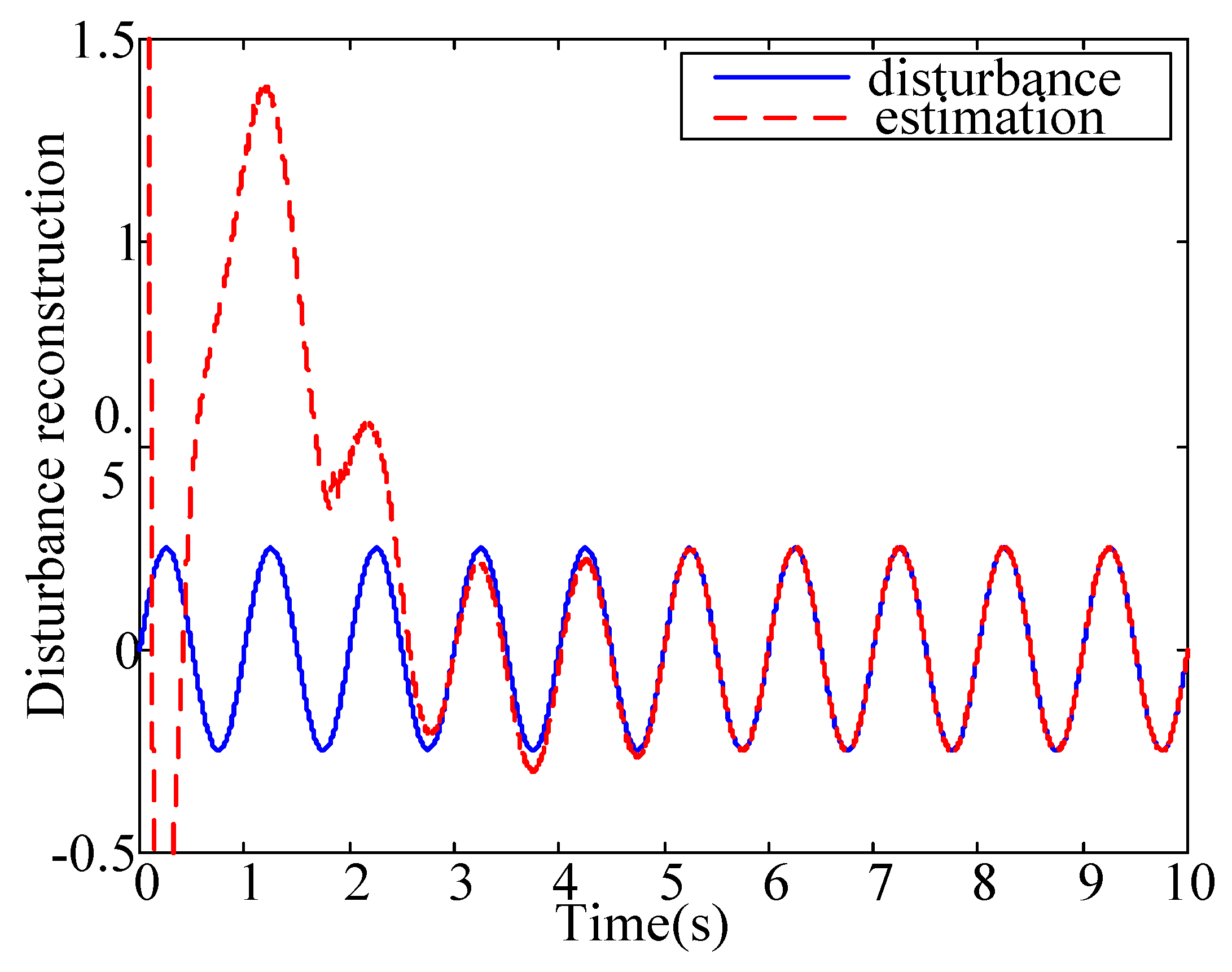
For the lumped perturbation term $f\left(x,t\right)$, there exists a positive constant $\zeta =1.8$ such that $\Vert D_{22}\dot{f}\left(x,t\right)\Vert \le \Vert D_{22}\Vert \left(\left|\frac{glM}{J_l}{x}_2\cos \left(x_1\right)\right|+\left|\dot{d}\left(t\right)\right|\right)\le \zeta =1.8$ and thereby the robust gains ${\xi }_i=2$ are considered. To compare with the method [22], in the following simulations, two types of external unknown inputs are considered to simulate $d\left(t\right)$. One is a continuous sine wave and the other is a discontinuous saw-tooth-like wave. 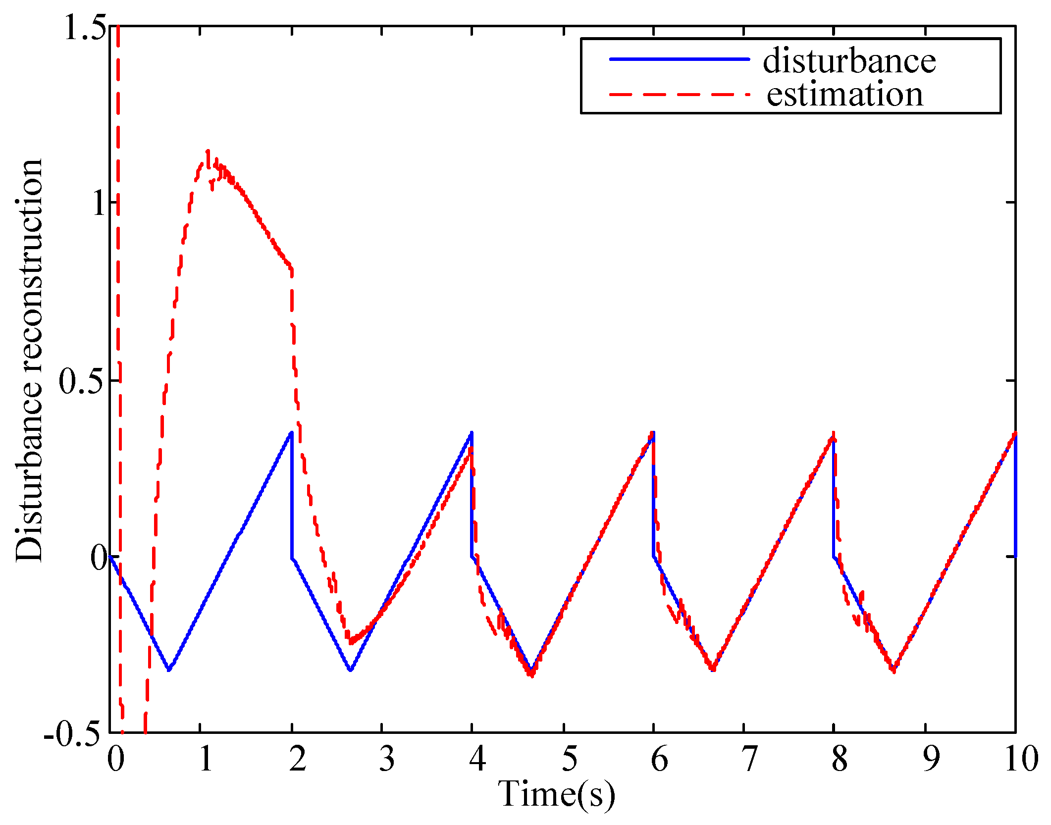The continuous unknown input is generated by $d\left(t\right)\equiv d_1\left(t\right)=0.25\sin \left(2\pi t\right)$ and the discontinuous one is generated by (using a Matlab script) $d\left(t\right)\equiv d_2\left(t\right)=0.025*\left(2\left|10t-20floor\left(0.5t\right)-6.5\right|-13\right)$. It is clear that the time derivative of the discontinuous one does not satisfy $L_2$ condition. However, the SMO can still recovery its profile accurately.

In the following simulations, the discontinuous control applied in the SMO is replaced by a sigmoid function [20,27]. The unknown input is estimated by considering the approximation: $v_{eq}\approx \rho \frac{P_{2}s}{\Vert P_{2}s\Vert +\epsilon }$ $\approx A_{21}{e}_1+D_{22}f\left(x,t\right)$, where $\rho =1$ and $\epsilon =0.005$ are used which lead to in $\eta \approx 0.89$.

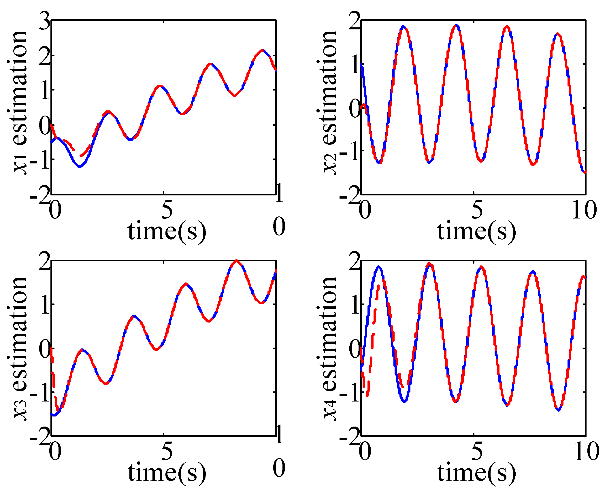
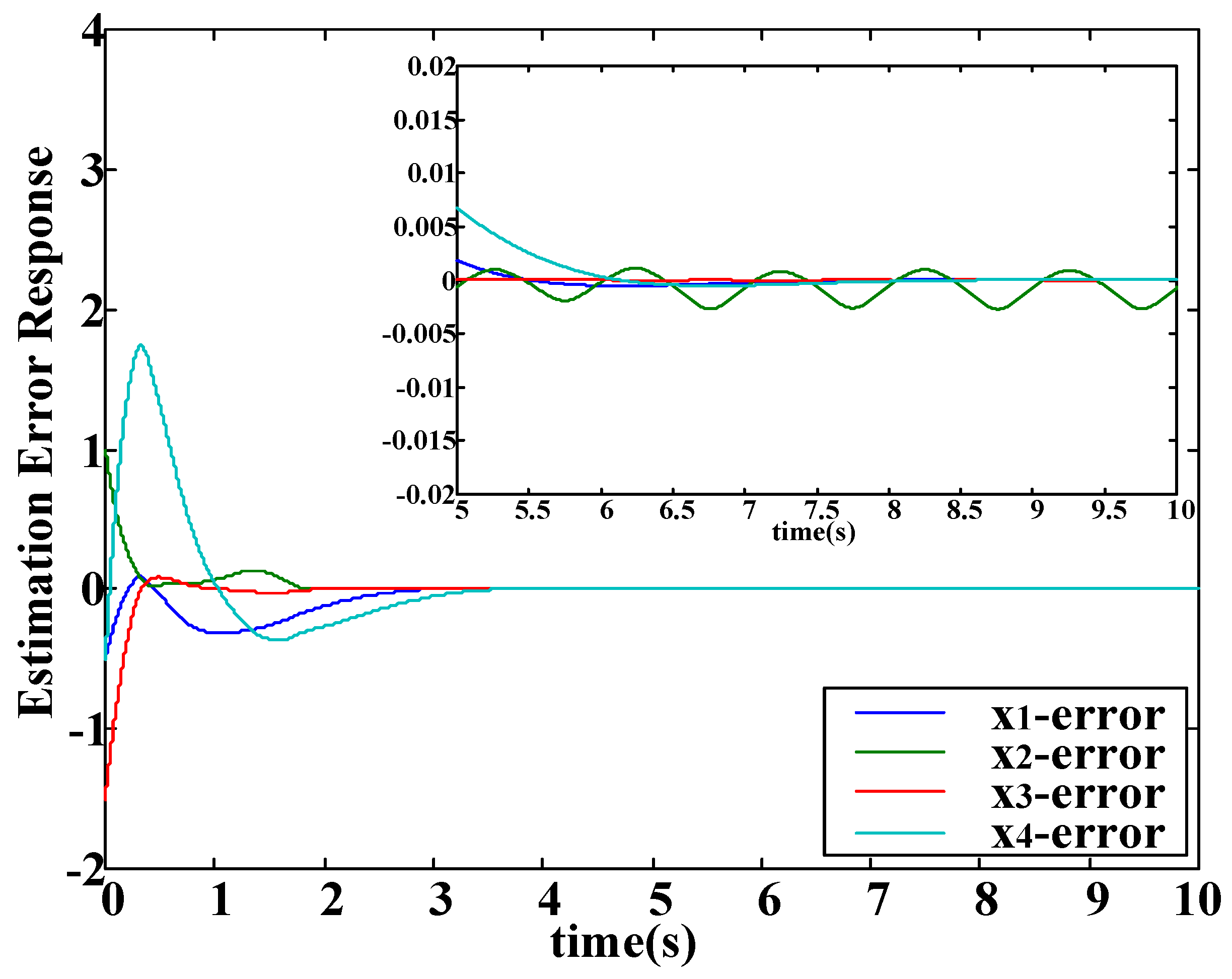
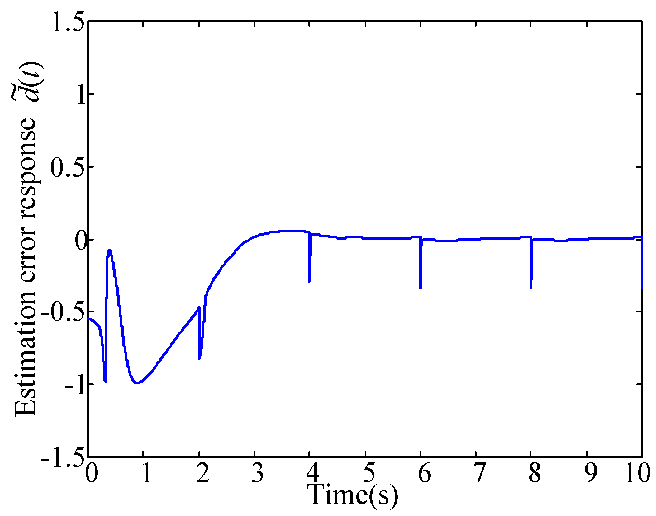
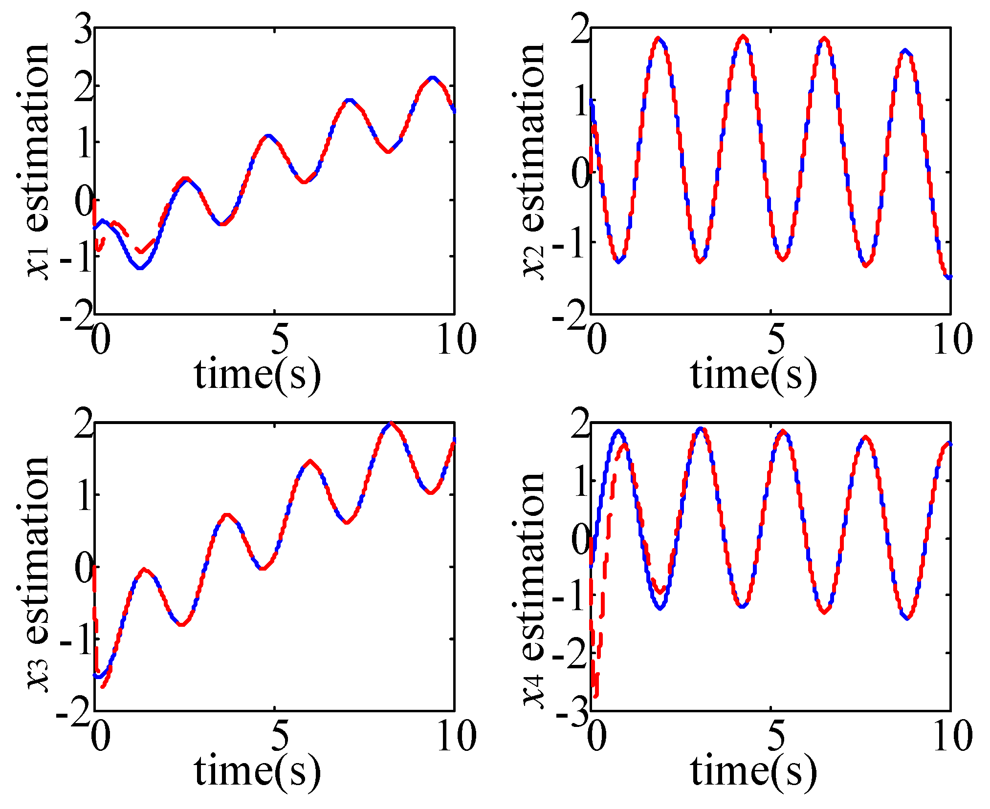
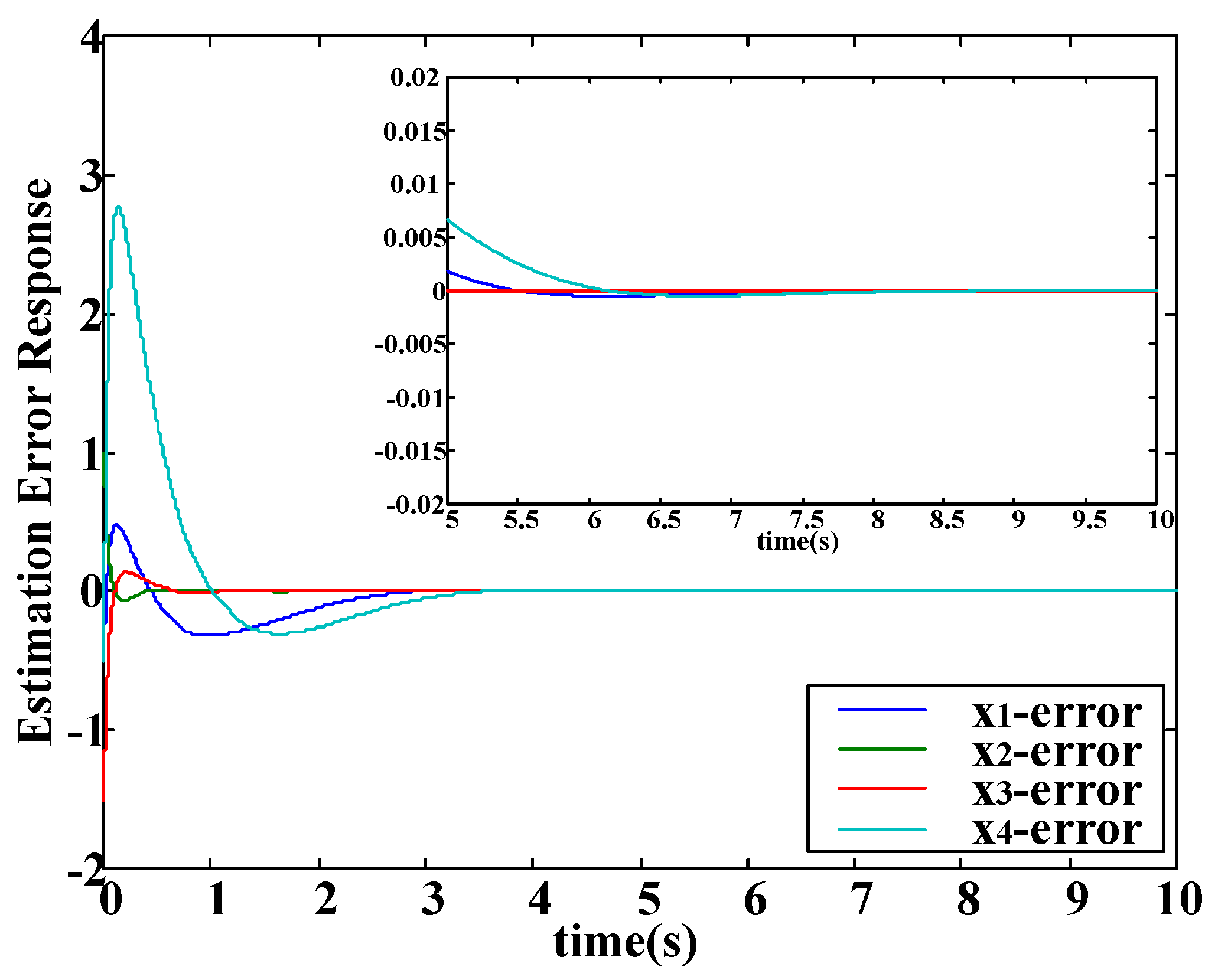
Figure 1 shows that the observer states approach to the real system states by using the SMO. The corresponding estimation errors are depicted in Figure 2. Note that the values of ${\tilde{x}}_2\left(t\right)$ are obviously larger than other state estimation errors. This is because that the unknown input directly affects in the direction of $x_2$ and the sigmoid-function-based control applied in the SMO cannot completely eliminate the unknown input.

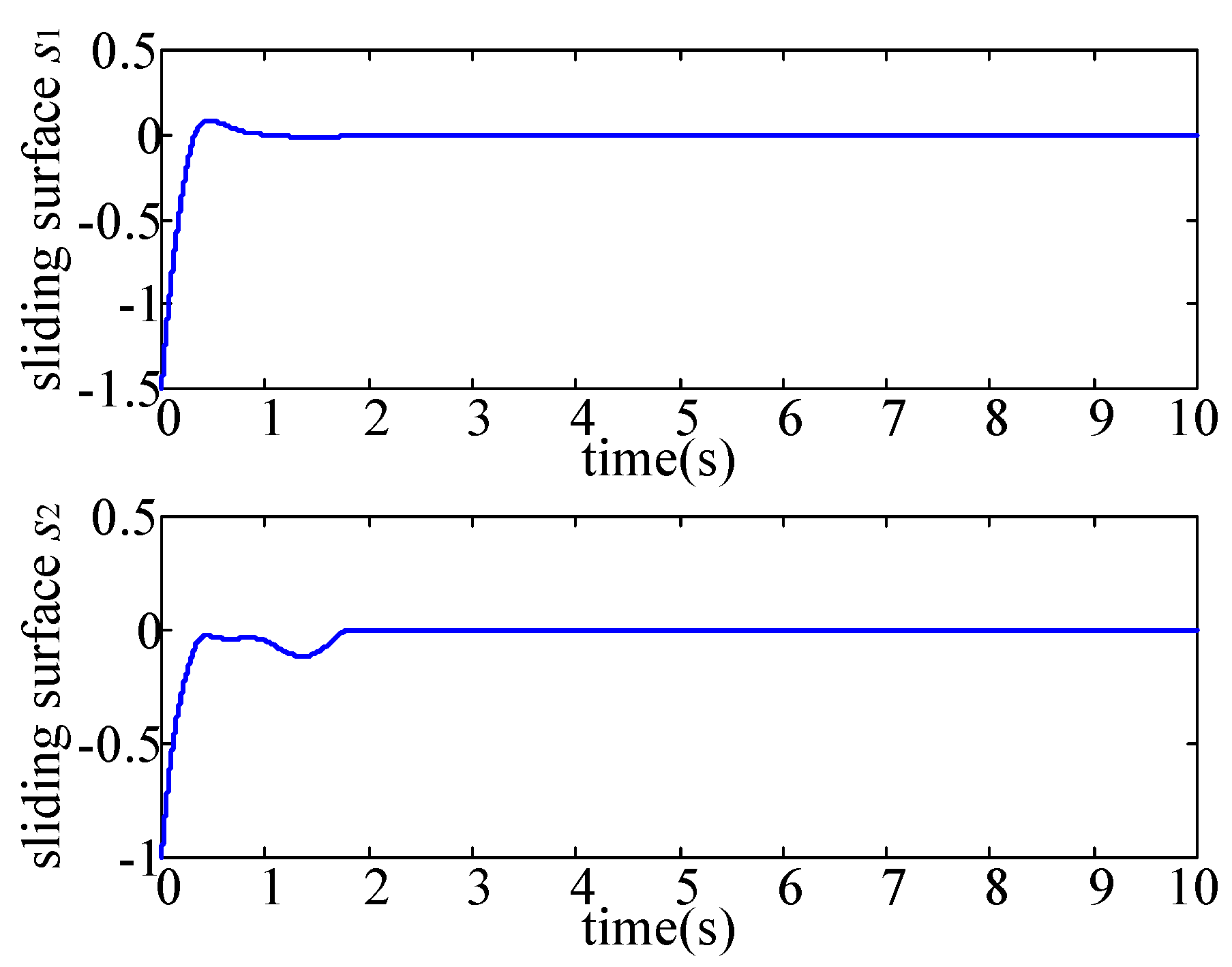
Examining the sliding trajectories as illustrated in Figure 3. It is obvious that the approaching phase does not occur immediately, but remains being realized in finite time under the approaching condition (33). Put it clearly, since the closed-loop observation error dynamics is exponentially stable, it follows that the circumstance $\Vert {\overline{A}}_{21}{e}_1\Vert <\eta$ is eventually achieved such that the approaching condition (33) is finally fulfilled. 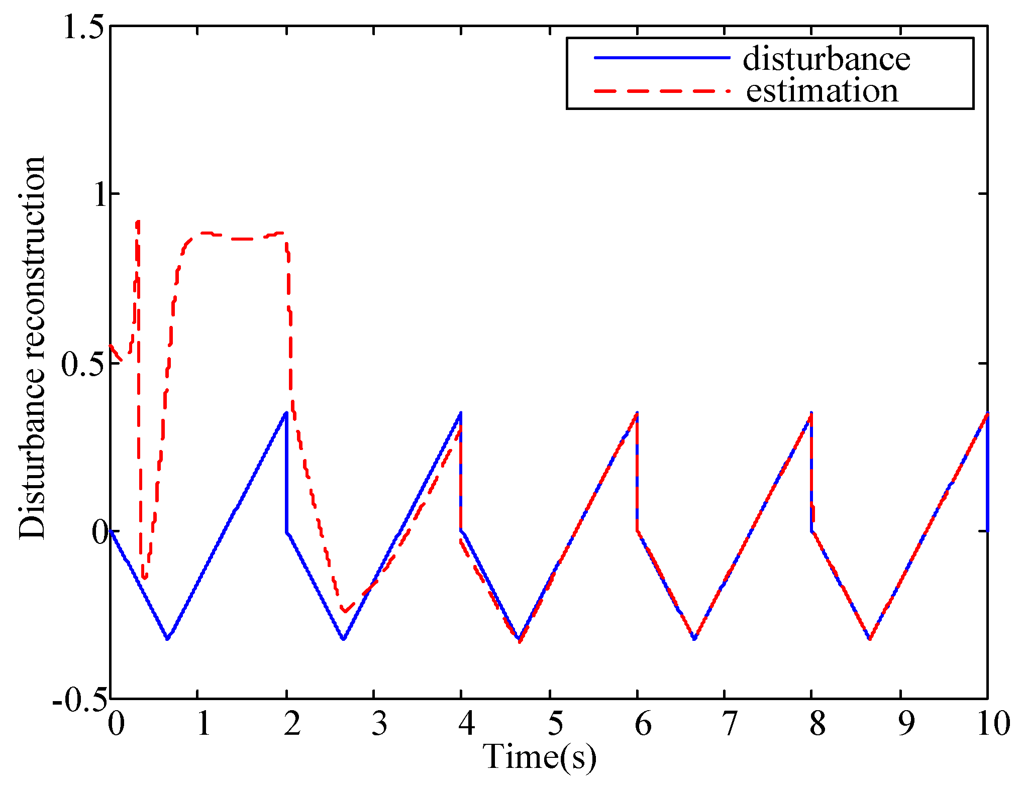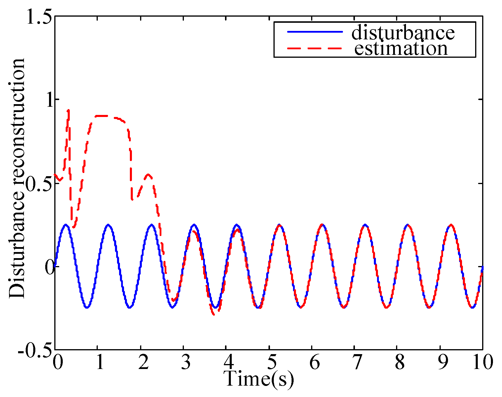Figure 4 demonstrates the unknown disturbance reconstruction by the way of equivalent control injection.

Figure 5, Figure 6 and Figure 7 are the results by using the proposed PIO. Different to Figure 2, the estimation performance can be further improved by using the proposed PIO. Figure 6 illustrates the main advantage of the PIO; that is, the perturbations are successfully eliminated. The disturbance recovery property is demonstrated in Figure 7. Detail comparison will be discussed later.

Figure 8, Figure 9, Figure 10 and Figure 11 are used to demonstrate the main difference between the SMO and the PIO for discontinuous unknown input reconstruction. Since the SMO is a class of discontinuous control strategy, it is able to reconstruct the non-smooth unknown input rapidly. Figure 8 and Figure 9 clearly show the fast recovery property of the SMO.

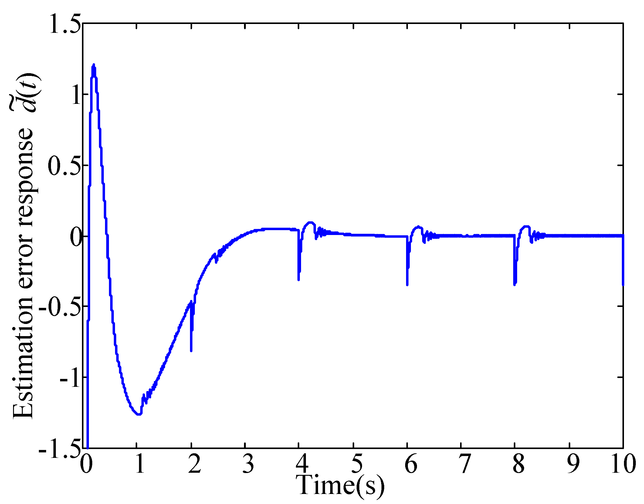
Figure 10 and Figure 11 illustrate that the control signals generated by PIO deviate from the true value of the unknown input at 2 s, 4 s, 6 s and 8 s. This because that the magnitude at these points changes with infinite fast speed, that is $\Vert D_{22}\dot{f}\left(x,t\right)\Vert \to \infty$. There is no continuous compensator can compensate such the critical situation. However, after these critical points, the time derivatives of the disturbance turn into finite and therefore the unknown input reconstruction can be successfully obtained.

To make quantitative comparison, the simulation results are summarized in

Table 2. Observation precision comparison ($t\ge 6$ s).

Performance Indices		$\mathbf{max}\left|{\tilde{\mathit{x}}}_1\left(\mathit{t}\right)\right|$	$\mathbf{max}\left|{\tilde{\mathit{x}}}_2\left(\mathit{t}\right)\right|$	$\mathbf{max}\left|{\tilde{\mathit{x}}}_3\left(\mathit{t}\right)\right|$	$\mathbf{max}\left|{\tilde{\mathit{x}}}_4\left(\mathit{t}\right)\right|$	$\mathbf{max}\left|\tilde{\mathit{d}}\left(\mathit{t}\right)\right|$
		$\frac{1}{\mathit{k}}{\displaystyle {\sum }_{\mathit{i}=1}^{\mathit{k}}\left|{\tilde{\mathit{x}}}_1\left(\mathit{t}\right)\right|}$	$\frac{1}{\mathit{k}}{\displaystyle {\sum }_{\mathit{i}=1}^{\mathit{k}}\left|{\tilde{\mathit{x}}}_2\left(\mathit{t}\right)\right|}$	$\frac{1}{\mathit{k}}{\displaystyle {\sum }_{\mathit{i}=1}^{\mathit{k}}\left|{\tilde{\mathit{x}}}_3\left(\mathit{t}\right)\right|}$	$\frac{1}{\mathit{k}}{\displaystyle {\sum }_{\mathit{i}=1}^{\mathit{k}}\left|{\tilde{\mathit{x}}}_4\left(\mathit{t}\right)\right|}$	$\frac{1}{\mathit{k}}{\displaystyle {\sum }_{\mathit{i}=1}^{\mathit{k}}\left|\tilde{\mathit{d}}\left(\mathit{t}\right)\right|}$
$d_1\left(t\right)$	SMO	5.3352 × 10−4	0.0027	5.2854 × 10−6	5.1507 × 10−4	0.0170
		1.4163 × 10−4	0.0012	2.1532 × 10−6	1.8376 × 10−4	0.0077
	PIO	5.3233 × 10−4	1.0138 × 10−6	1.3686 × 10−6	5.1937 × 10−4	0.0048
		1.4084 × 10−4	9.3354 × 10−8	2.1170 × 10−7	1.8101 × 10−4	0.0017
$d_2\left(t\right)$	SMO	5.3181 × 10−4	0.0032	5.8621 × 10−6	5.1517 × 10−4	0.3389
		1.4173 × 10−4	0.0013	1.9428 × 10−6	1.8237 × 10−4	0.0068
	PIO	5.3245 × 10−4	0.0103	8.7710 × 10−7	5.1956 × 10−4	0.3517
		1.4084 × 10−4	8.6742 × 10−4	1.4003 × 10−7	1.8100 × 10−4	0.0126

. Table 2 contains two categories: the first one is the estimation precision comparison for system subject to continuous unknown input and the second one is for system suffering the discontinuous one. For system with continuous disturbance $d_1\left(t\right)$, simulation results show that the estimation conducted by applying the PIO is better than those obtained by using the SMO. In contrast, when system is subject to discontinuous disturbance $d_2\left(t\right)$, SMO can still reach fast estimation even though the disturbance is not differentiable and the $L_2$ condition for the signal time derivative is not satisfied [22]. Therefore, the input reconstruction performance by SMO is better than those by PIO in the sense of maximum estimate errors. However, it is argued that most of disturbances in the real world are continuous and no continuous control effort is capable of precisely eliminating discontinuous disturbances. As a result, under this circumstance the resulting estimation performances conducted by the PIO will be better than those conducted by the SMO. Additionally, since no discontinuous control component is directly applied in the PIO, the robust integral type observer will be an adequate choice for bandwidth limited hardware realizations.

5. Conclusions

This paper has proposed robust observer designs for a class of nonlinear systems. In order to achieve precise state estimation and unknown input reconstruction simultaneously, designs of the SMO and the PIO are subject to specific system structures. Sufficient conditions for the existence of the robust observers are characterized in terms of LMIs. Therefore, the observer gains could be easily and efficiently determined. For systems subject to continuous unknown input, the PIO is capable of estimating system states precisely as well as recovering unknown input. For systems subject to discontinuous unknown input, the SMO can reach fast disturbance estimation. Moreover, there are no specific forms imposed on the unknown inputs, and hence the application varieties can be extended. Finally, applications of the proposed SMO and the PIO for a single link flexible robot arm are given to demonstrate the state estimation as well as the unknown input reconstruction properties.