Article

Extended Backstepping Sliding Controller Design for Chattering Attenuation and Its Application for Servo Motor Control

Department of Aeronautics and Astronautics, National Cheng Kung University, Tainan 701, Taiwan
*
Author to whom correspondence should be addressed.
Appl. Sci. 2017, 7(3), 220; https://doi.org/10.3390/app7030220
Submission received: 12 November 2016 / Revised: 10 February 2017 / Accepted: 14 February 2017 / Published: 27 February 2017
(This article belongs to the Special Issue Selected Papers from the 2016 International Conference on Inventions)

Abstract

:
This paper presents a robust backstepping design for motion control in the presence of model uncertainties and exogenous disturbances. The main difficulty in dealing with motion control is to reduce the effect of friction, which exists in the moving mechanism and induces nonlinear behavior. In this study, the friction dynamic is considered as the external disturbance, and the proposed backstepping control algorithm is integrated with the sliding mode control, so that the effect of matching disturbances can be eliminated. The proposed approach guarantees the system asymptotic stability, globally, without significant chatter. Therefore, the developed algorithm can be realized for practical manufacturing motion control stages. Experiments including positioning and tracking controls are conducted to demonstrate the feasibility of the proposed method.

1. Introduction

Backstepping design is a systematic recursive design procedure based on the choice of a Lyapunov function. This approach is suitable for the design of a class of nonlinear systems in the strict feedback form. In the design procedure, the system variable is treated as an independent (or a fictitious) input for subsystems, and consequently, each step results in an updated control design for the next step. The control law for each step is refined with the satisfaction of the Lyapunov function, such that the stability for each subsystem can be guaranteed as outlined in [1]. In the traditional backstepping design, system robustness can be maintained by using high gain control (under the condition that the system uncertainties are state dependent). However, in the case of a motion system, the system may be subject not only to uncertain parameters, but also to un-modeled system dynamics; which is state independent, such that the high gain backstepping design may not result in the asymptotic stability of such a system.
In recent years, several control strategies, such as adaptive control [2,3,4], sliding mode control [5,6] and neural networks [7,8], have been integrated into the logical backstepping design procedure in order to enhance system robustness. An integral action has been widely used in adaptive backstepping control for eliminating steady state error, while a smooth sign function was adopted for avoiding chatter in sliding mode control. Some nonlinear functions can be estimated using neural networks with a backstepping design scheme. Other robust backstepping control approaches for specific nonlinearities, such as system time delays [9], mismatched uncertainties [10], backlash-like hysteresis [11] and input uncertainties [12], were also developed to make the resulting system insensitive to model uncertainties and external disturbances. Moreover, in recent studies [13,14,15,16], it has been demonstrated that the backstepping controller design concept can be applied for different nonlinear systems. However, only numerical simulations were provided. In this paper, this design concept is applied for the control of a servo mechanical system. Not only the theoretical derivation is given, both the numerical simulations and experimental verifications are addressed, as well, to verify the feasibility of the proposed method. In regard to [15], the authors proposed an integral type robust controller based on the sliding control design concept. However, the controllers cannot attain the so-called approaching/sliding conditions, so the stability proof will be relatively complicated.
One of the main difficulties in dealing with motion control is to suppress the effect of friction, which exists in the moving mechanism. Two main kinds of friction behavior have been observed experimentally in the literature, namely the Stribeck effect and hysteresis [17], occurring in sliding and pre-sliding regions, respectively. These nonlinear properties of friction induce undesirable behavior that includes steady state positioning errors, tracking lags, limit cycles and stick-slip motion. In the recent decade, friction model-based compensation approaches and the disturbance observer have been widely adopted for motion control problems [18,19,20,21,22]. Due to the complexity of friction, recently, a nonlinear damping-based backstepping design was proposed, where the friction effect is taken as a nonlinear function and is going to be measured by a time delay estimate (TDE) [23]. Then, the control performance is further enhanced by considering the TDE together with an internal model control [24].
However, the friction behavior is a highly nonlinear phenomenon, which is difficult to be well described, especially for the inter-medium region between static friction [25] and dynamic friction. Even though there were several friction models in the literature, they can only be applied for specific friction regions. It is difficult to obtain quantitative analysis of friction due to its time and position varying nature. In some cases, an inaccurate friction model would likely induce an additional control payload. Therefore, in this work, the LuGre model [26] is considered, but no extra estimator [23,24], friction observer [27] or adaption law [28] is applied. Designers only have to deal with a pair liner gain and a robust gain. To relax the implementation effort, only the upper bound of the variation on the lumped perturbation is needed to adjust the control gain w. Therefore, based on the robust stability property, one can gradually increase the value of the robust gain to achieve a satisfactory result. From the end-user point of view, less control parameters are able to achieve a more user-friendly environment for control tuning.
To preserve the approaching/sliding conditions in the traditional sliding mode control (SMC), as well as ease the control discontinuity, this paper develops an extended backstepping sliding mode control (EBSMC) algorithm, which provides global stability of the system without including an additional compensator or observer. Moreover, it will be shown that the proposed controller turns into a robust PD controller once a robust gain is set to be zero. Under this circumstance, the robust stability issue is going to be addressed by using some linear matrix inequalities (LMIs). Finally, the effectiveness of the developed control strategy is verified through numerical and experimental studies.

2. Proposition of EBSMC

The LuGre model, which is capable of describing most friction phenomena, was proposed by Canudas et al. [26]. This model states that once relative motion occurs between two surfaces, friction force is caused by the deflection of bristles on those surfaces.
Consider the following motion system with friction:
M x ¨ p = u F d
where M is the system mass, x p is the system position and u is the applied force. Moreover, F and d are the friction force and an external load, respectively. The friction force described by the LuGre model is comprised of two components. One originates from the bristle behavior defined as F B ( κ , κ ˙ ) , and the other is due to the viscous effect F V , that is:
F = F B ( κ , κ ˙ ) + F V
where F B ( κ , κ ˙ ) = σ 0 κ + σ 1 κ ˙ and F V = σ 2 x ˙ p . σ 0 is the stiffness coefficient; σ 1 is the damping coefficient; and σ 2 is the viscous coefficient. κ is the deflection of the bristle, and its variation is defined as follows:
κ ˙ = x ˙ p | x ˙ p | G ( x ˙ p ) κ
where σ 0 G ( x ˙ p ) = f C + ( f S f C ) exp [ ( x ˙ p / v S ) N ] . f C is the Coulomb friction, and f S is the maximum static friction; v S is the Stribeck velocity; and the positive factor N is employed in modifying the transition curve of friction at low velocity.
Define tracking error as e 1 = x d x p and e 2 = e ˙ 1 = x ˙ d x ˙ p , where x d is the desired position. Then, the system in the form of error dynamics becomes:
e ˙ 1 = e 2 e ˙ 2 = σ 2 M e 2 1 M u + σ 2 M x ˙ d + x ¨ d + 1 M F B ( κ , κ ˙ ) + d
Define a virtual state e 3 = e ˙ 2 ; the system (4) can then be represented as the following extended third order extended dynamic system [29]:
e ˙ 1 = e 2 e ˙ 2 = e 3 e ˙ 3 = σ 2 M e 3 1 M u ˙ + σ 2 M x ¨ d + x d + 1 M F ˙ B ( κ , κ ˙ ) + d ˙
The proposed EBSMC design procedure for System (5) is described as follows.
Step 1:
By choosing the nominal control effort u ˙ of the extended system as:
u ˙ = σ ^ 2 e 3 + σ ^ 2 x ¨ d + M ^ x d M ^ u ˙ C
where M ^ and σ ^ 2 are the nominal values of system mass and viscous coefficient, respectively. Then, the extended system in (5) can be formulated as:
e ˙ 1 = e 2 e ˙ 2 = e 3 e ˙ 3 = u ˙ C + D ˜ ˙ ( e 3 , x ¨ d , x d , u ˙ C , F ˙ B ( κ , κ ˙ ) , d ˙ )
where D ˜ ˙ ( e 3 , x ¨ d , x d , u ˙ C , F ˙ B ( κ , κ ˙ ) ) = 1 M [ σ ˜ 2 e 3 + σ ˜ 2 x ¨ d + M ˜ x d M ˜ u ˙ C + F ˙ B ( κ , κ ˙ ) + d ˙ ] denotes the lumped system perturbations. Note that M = M ^ + M ˜ and σ 2 = σ ^ 2 + σ ˜ 2 .
For the servo motor, since the maximum applied force is limited, the resulting speed, acceleration and jerk are also limited. Therefore, it is reasonable to assume that there exists a positive constant η that satisfies η = sup | D ˜ ˙ ( e 3 , x ¨ d , x d , u ˙ C , F ˙ B ( κ , κ ˙ ) , d ˙ ) | > 0 . The detailed proof can be found in the Appendix A.
Consider the system state e 2 as an independent input, and let:
e 2 = ϕ 1 ( e 1 ) = k 1 e 1 ,   k 1 > 0 .
Select a Lyapunov function V B 1 = 1 2 e 1 2 . It can then be obtained that:
V ˙ B 1 = e 1 e ˙ 1 = k 1 e 1 2 0
Therefore, state e 1 is asymptotically stable.
Step 2:
Actually, there may be differences between e 2 and ϕ 1 ( e 1 ) . Therefore, a new error variable z 1 = e 2 ϕ 1 ( e 1 ) is defined, which presents the difference between the stabilizing control law ϕ 1 ( e 1 ) and the error state e 2 . By adding and subtracting the virtual control law ϕ 1 ( e 1 ) to the first equation of (7), we can get the dynamic of the subsystem ( e 1 ) as follows:
e ˙ 1 = ϕ 1 ( e 1 ) + [ e 2 ϕ 1 ( e 1 ) ] = ϕ 1 ( e 1 ) + z 1
Equations (8) and (9) can be satisfied if z 1 in (10) equals zero. Further, consider the dynamic of z 1 :
z ˙ 1 = e ˙ 2 ϕ ˙ 1 ( e 1 ) = e 3 ϕ ˙ 1 ( e 1 )
In a similar manner, treat the state e 3 as an independent input of the form ϕ 2 ( e 1 , z 1 ) as the following:
e 3 = ϕ 2 ( e 1 , z 1 ) = e 1 k 2 z 1 + ϕ ˙ 1 ( e 1 ) ,   k 2 > 0 .
Select a Lyapunov function of the subsystem ( e 1 , z 1 ) in the form of:
V B 2 = V B 1 + 1 2 z 1 2 = 1 2 e 1 2 + 1 2 z 1 2
From (10)–(12), the derivative of (13) is obtained as:
V ˙ B 2 = e 1 e ˙ 1 + z 1 z ˙ 1 = k 1 e 1 2 k 2 z 1 2 0
Thus, the subsystem ( e 1 , z 1 ) is asymptotically stable.
Step 3:
By adding and subtracting the virtual control law ϕ 2 ( e 1 , z 1 ) to (11) and defining an error variable as z 2 = e 3 ϕ 2 ( e 1 , z 1 ) , (11) can then be represented as:
z ˙ 1 = [ e 3 ϕ 2 ( e 1 , z 1 ) ] + ϕ 2 ( e 1 , z 1 ) ϕ ˙ 1 ( e 1 ) = z 2 + ϕ 2 ( e 1 , z 1 ) ϕ ˙ 1 ( e 1 )
and:
z ˙ 2 = e ˙ 3 ϕ ˙ 2 ( e 1 , z 1 ) = u ˙ C ϕ ˙ 2 ( e 1 , z 1 ) + D ˜ ˙ ( e 3 , x ¨ d , x d , u ˙ C , F ˙ B ( κ , κ ˙ ) , d ˙ )
From Step 1 and Step 2, it is found that the desired behavior of the subsystem ( e 1 , z 1 ) can be achieved if the condition z 2 = 0 is satisfied. Therefore, the control purpose can be simplified to the regulation of the virtual state z 2 in the presence of external disturbances. The sliding mode control can be introduced to the backstepping design as follows.
Select a sliding surface of:
S = z 2
In the absence of D ˜ ˙ in (16), the corresponding equivalent control force can be obtained by S ˙ = 0 , that is:
u ˙ C e q = ϕ ˙ 2 ( e 1 , z 1 )
A switching control action is applied to enhance the system robustness, such that system states stay on the sliding surface even in the presence of disturbances:
u ˙ C = u ˙ C e q w sgn ( S )
where the robust gain w satisfies the condition w > η .
Choose a Lyapunov function as V S = S 2 / 2 , and it can be obtained that:
V ˙ S = S [ u ˙ C ϕ ˙ 2 ( e 1 , z 1 ) + D ˜ ˙ ( e 3 , x ¨ d , x d , u ˙ C , F ˙ B ( κ , κ ˙ ) , d ˙ ) ] = S [ w sgn ( S ) + D ˜ ˙ ( e 3 , x ¨ d , x d , u ˙ C , F ˙ B ( κ , κ ˙ ) , d ˙ ) ] | S | [ w η ] 0
It shows that the approaching condition can be reached, and thus, the system is asymptotically stable.
For the final implementation, substituting (19) into (6), the integral type control effort for the original second order system can be represented as:
u = σ ^ 2 e 2 + σ ^ 2 x ˙ d + M ^ x ¨ d M ^ 0 t ( u ˙ C e q w sgn ( S ) ) d τ
Represent (21) in the form of error states:
u = M ^ ( 1 + k 1 k 2 ) e 1 + M ^ ( k 1 + k 2 ) e 2 σ ^ 2 e 2 + σ ^ 2 x ˙ d + M ^ x ¨ d + M ^ w 0 t sgn ( S ) d τ
Further, substitute (22) into (4); it results:
e ˙ 2 = σ 2 M e 2 1 M u + σ 2 M x ˙ d + x ¨ d + 1 M F B ( κ , κ ˙ ) = σ 2 M e 2 1 M [ M ^ ( 1 + k 1 k 2 ) e 1 + M ^ ( k 1 + k 2 ) e 2 σ ^ 2 e 2 + σ ^ 2 x ˙ d + M ^ x ¨ d + M ^ w 0 t sgn ( S ) d τ ] + σ 2 M x ˙ d + x ¨ d + 1 M F B ( κ , κ ˙ ) + 1 M d = ( 1 + k 1 k 2 ) e 1 ( k 1 + k 2 ) e 2 + D ˜ ( e 2 , x ˙ d , x ¨ d , u C , F B ( κ , κ ˙ ) , d ) w 0 t sgn ( S ) d τ
From (17), the sliding mode dynamics can be represented as:
S = e ˙ 2 + ( k 1 + k 2 ) e 2 + ( 1 + k 1 k 2 ) e 1 = D ˜ ( e 2 , x ˙ d , x ¨ d , u C , F B ( κ , κ ˙ ) , d ) w 0 t sgn ( S ) d τ
Remark 1.
According to (20), the robust gain w can be applied to maintain the sliding motion even when the system is subject to disturbances. This reveals that the lumped perturbation D ˜ in (24) can be compensated by the nonlinear integral action, and thereby, the exponential stability of the system can be achieved by a proper choice of gain k 2 and k 1 used in (22).
Remark 2.
The closed-loop system robustness against system uncertainties, as well as unknown exogenous disturbances is achieved by a suitable adjustment of a single robust gain w. When an insufficient large value is applied, the condition (20) may not be attained. Under this circumstance, for example, a critical case that w = 0, one has e ˙ 2 + ( k 1 + k 2 ) e 2 + ( 1 + k 1 k 2 ) e 1 = D ˜ . Roughly speaking, the closed-loop system is stable by means of bounded-input bounded-output stability (BIBO). In the Appendix A, robust gain estimation and the robust stability issue are going to be addressed further. Based on the achievement of robust stability, one can increase the value of w gradually to achieve desired control performance without inducing unstable behavior.

3. Simulation Results

For general controller design and system physical behavior validation purposes, system parameters need to be identified in advance [30]. In Section 2, the proposed control law (22) involves part of the system nominal parameters, including system mass and viscous coefficient. A systematic estimation method is going to present in the following.
For the servo system with apparent velocity, the main contribution of the friction effect comes from Coulomb friction and the viscous coefficient; that is, F σ 2 v + f C s i g n ( v ) , where v = x ˙ p .
Reconsider (1) in the absence of external disturbance; one has:
M d v d t = u ( σ 2 v + f C s i g n ( v ) )
From the practical realization point of view, the corresponding discrete model can be directly derived by taking the backward difference:
d v d t v ( k ) v ( k 1 ) T s
where T s denotes as the sampling period.
Hence, the dynamic Equation (25) can be approximated by:
v ( k ) = M M + σ 2 T s v ( k 1 ) + T s M + σ 2 T s u ( k ) + f C T s M + σ 2 T s s i g n ( v ( k ) )
Based on several measurements, (27) can be represented by:
[ v ( k ) v ( k + 1 ) v ( k + m ) ] = [ v ( k 1 ) F ( k ) s i g n ( v ( k ) ) v ( k ) F ( k + 1 ) s i g n ( v ( k + 1 ) ) v ( k + m 1 ) F ( k + m ) s i g n ( v ( k + m ) ) ] [ X 1 X 2 X 3 ]
where:
X 1 = M M + σ 2 T s ,   X 2 = T s M + σ 2 T s ,   X 3 = f C T s M + σ 2 T s
Define:
Y = [ v ( k ) v ( k + 1 ) v ( k + m ) ] , A = [ v ( k 1 ) F ( k ) s i g n ( v ( k ) ) v ( k ) F ( k + 1 ) s i g n ( v ( k + 1 ) ) v ( k + m 1 ) F ( k + m ) s i g n ( v ( k + m ) ) ] , X = [ X 1 X 2 X 3 ]
The optimal solution is:
X o p t X = ( A T A ) 1 A T Y
Therefore, the servo motor parameters can be calculated by:
M = X 1 X 2 T s ,   σ 2 = 1 X 1 X 2 ,   f C = X 3 X 2
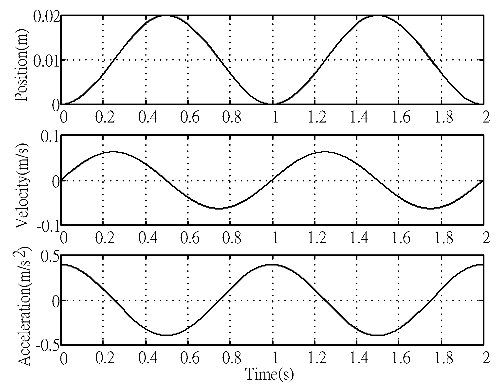
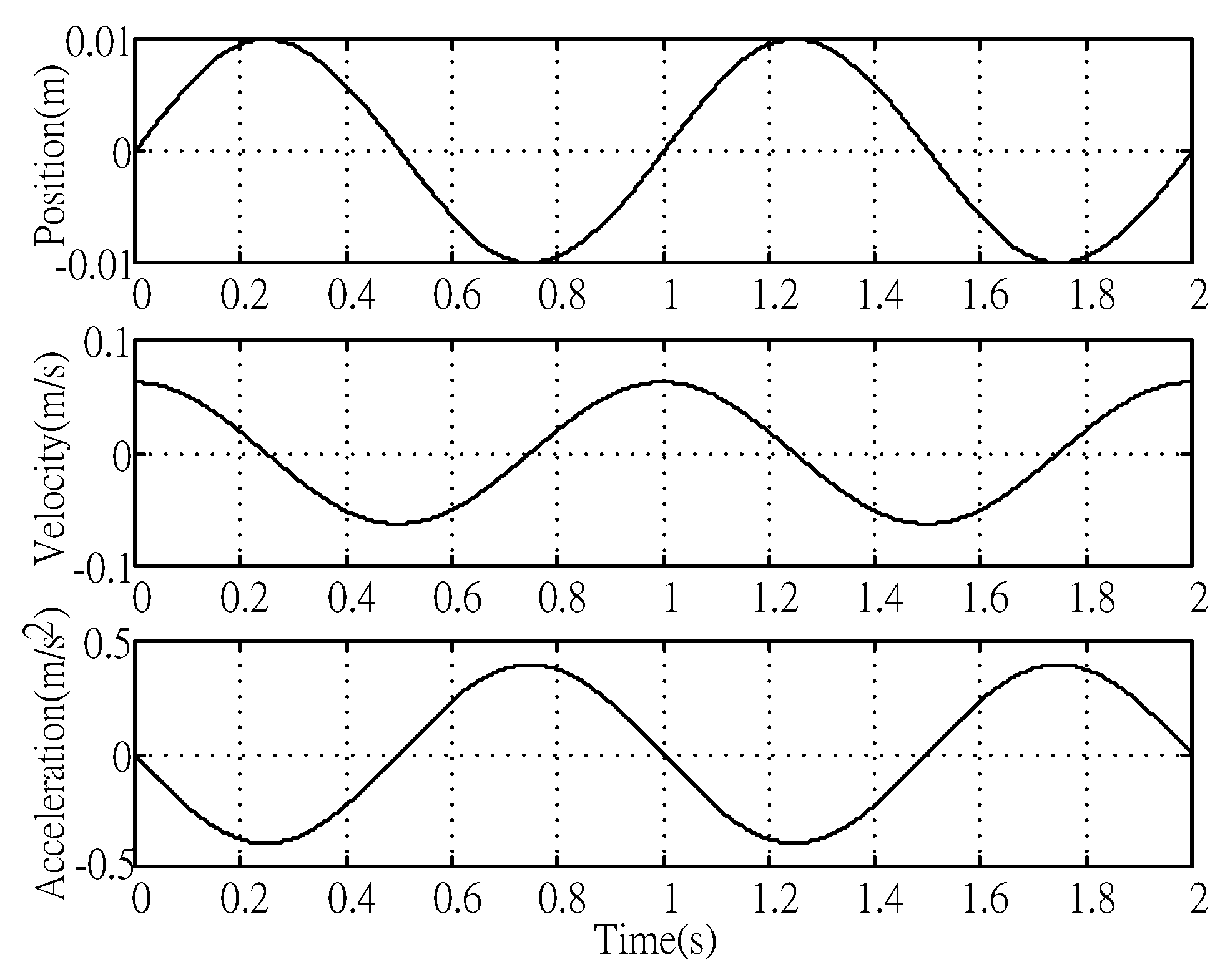
In the following simulation study, periodical reference commands of the form x d = x d 1 = R sin ( 2 π f t ) shown in Figure 1 and x d = x d 2 = R [ 1 + sin ( 2 π f t + 1.5 π ) ] shown in Figure 2 were adopted. The simulation results were performed by MATLAB code ode45 (Runge–Kutta method) with maximum step size 0.000025 (s). The same control gains were used for both cases and are listed in Table 1. 
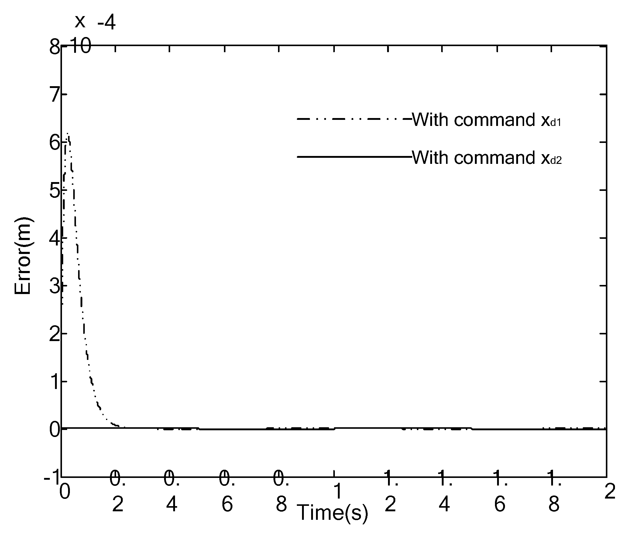
Figure 3 is the comparison of tracking performance. It can be found that the tracking error with x d 1 is comparatively large at the beginning of control process, which is caused by initial velocity error, but this phenomenon can be avoided with x d 2 . The tracking error is of the order 10−7 in the simulation, which is caused by the finite time switching numerical simulation and can be totally eliminated from the continuous case. 
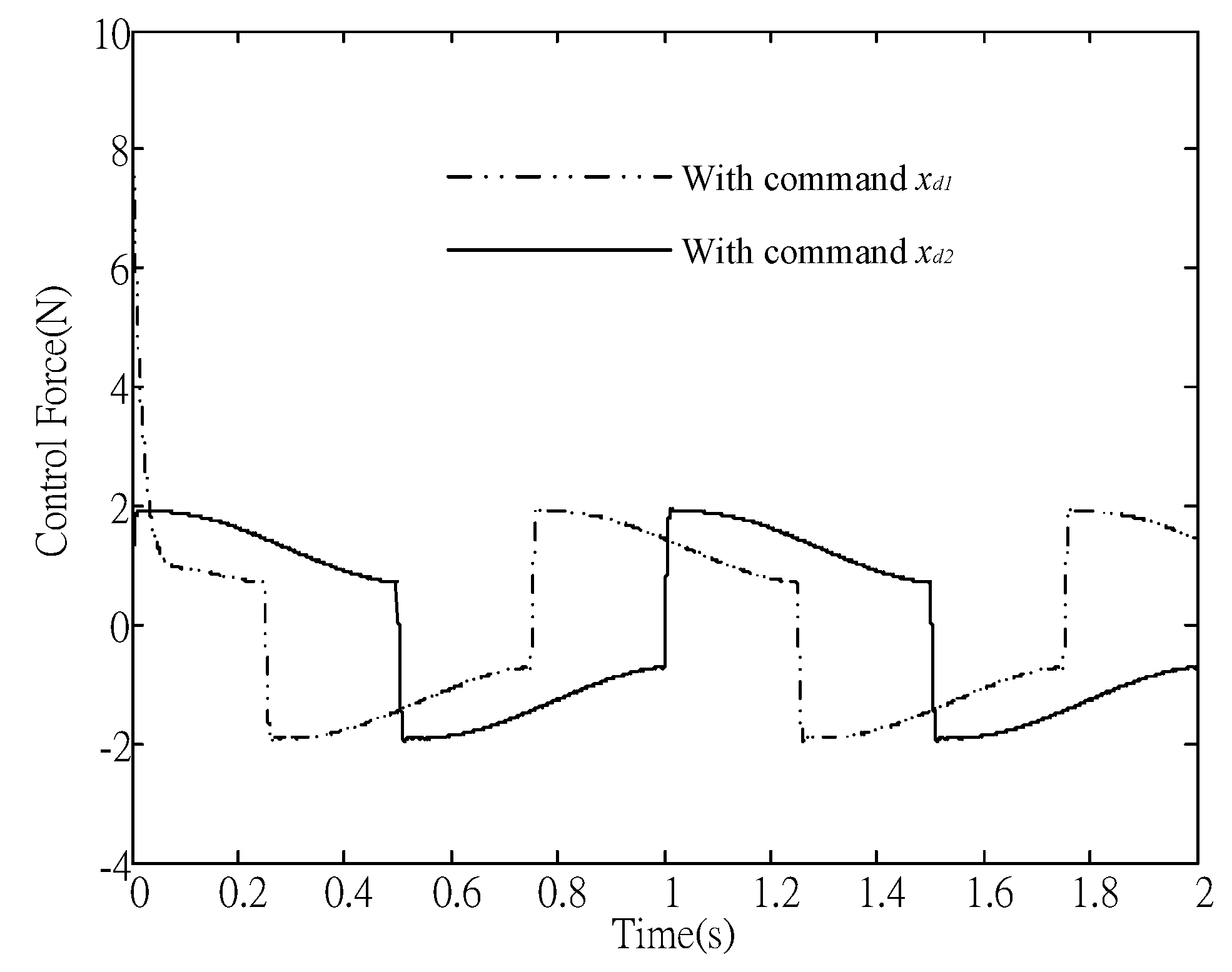
Figure 4 is the corresponding control force for both cases. A larger control force was caused by the reference x d 1 from non-zero desired initial velocity. According to (27), the gain w required to force the state on the sliding surface is 395,640 and 603 for x d 1 and x d 2 , respectively. For illustrative purposes, w = 603 is applied for both cases. 
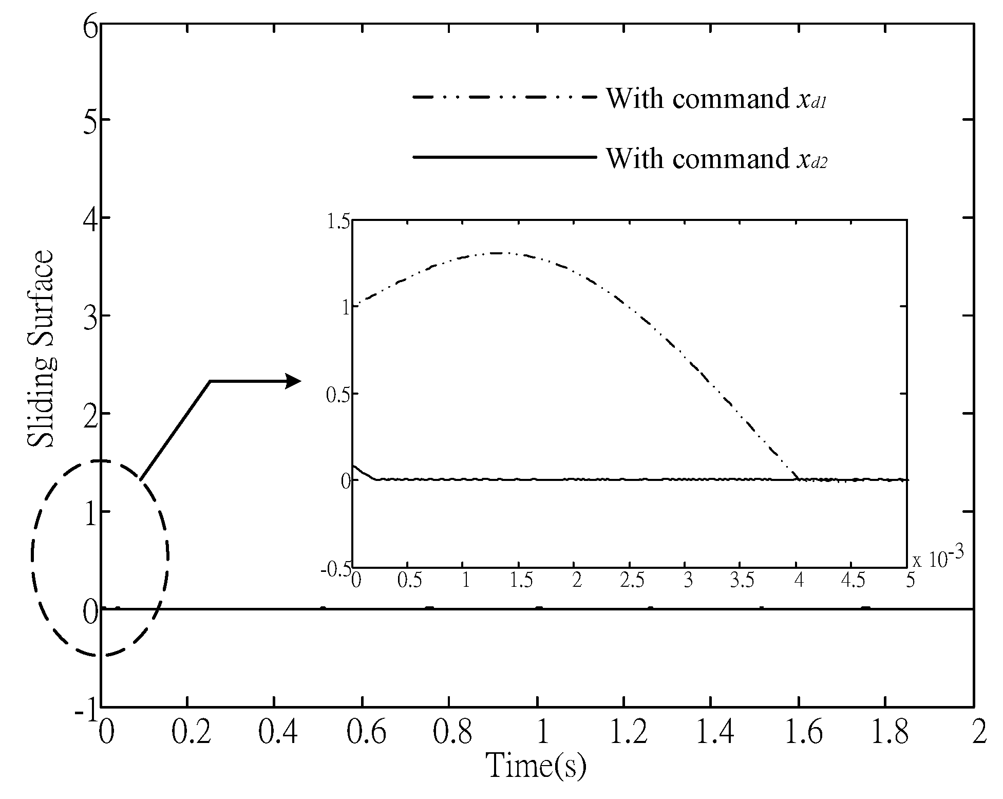
Figure 5 shows that the state stays on the sliding surface for x d = x d 2 , but not for x d = x d 1 , even though the steady state tracking error was eliminated for both cases. To bound the system state on S = 0 for non-zero initial velocity, the approaching condition can only be achieved using a sufficiently large gain w, which may cause the controller saturation. The initial reference commands play an important role in tracking control, which is true when applying other control strategies.
Next, a comparison study on the PID controller and the proposed EBSMC is presented. It is well known that for tracking applications, larger tracking errors are usually induced when motions change direction. During the velocity reversal, the variation of the nonlinear friction forces is apparently fast such that the linear controller (PID) is not able to overcome the perturbations properly for this critical situation.
For the motion control system, the error dynamics can be represented by:
e ˙ 1 = e 2 e ˙ 2 = σ 2 M e 2 1 M u + σ 2 M x ˙ d + x ¨ d + 1 M F B ( κ , κ ˙ ) + 1 M d
Consider (22), but now, the control algorithm is modified in the form of a PID controller:
u = M ^ K P e 1 + M ^ K D e 2 σ ^ 2 e 2 + σ ^ 2 x ˙ d + M ^ x ¨ d + M ^ K I 0 t e 1 d τ
Substituting (34) into (33) yields:
e ˙ 1 = e 2 e ˙ 2 = K P e 1 K D e 2 K I 0 t e 1 d τ + Γ
where:
Γ = M ˜ M K P e 1 + M ˜ M K D e 2 + M ˜ M K I 0 t e 1 d τ σ ˜ 2 M e 2 + σ ˜ 2 M x ˙ d + ( 1 M ˜ M ) x ¨ d + 1 M F B ( κ , κ ˙ ) + 1 M d
To address the closed-loop stability and control performance of (35), let e ˙ 1 = e 2 and e ˙ 2 = e 3 ; one can derive the following augmented system:
e ˙ a = ( A a + Δ A a ) e a + Γ a
where e a = [ e 1 e 2 e 3 ] T and:
A a = [ 0 1 0 0 0 1 K I K P K D ] , Δ A a = [ 0 1 0 0 0 1 M ˜ M K I M ˜ M K P 1 M ( M ˜ K D σ ˜ 2 ) ] Γ a = [ 0 0 σ ˜ 2 M x ¨ d + ( 1 M ˜ M ) x d + 1 M F ˙ B ( κ , κ ˙ ) + 1 M d ˙ ]
It is clear that the control issue turns into a robust stabilization problem, and the stability issue can also be solved by ways of LMIs. Similar to the steps from (47) to (56), it is easy to show that by the properly selected triple ( K P , K I , K D ) , there must exist a region Φ , such that:
e a Φ : = 2 λ max ( P ) λ min ( Q ) Γ a
Equation (39) implies that the control performance is relevant to the size of Γ a . Even though the variation of the lumped perturbation is finite, the PID control precision is going to be limited by the magnitude of the variation. In other words, better tracking performance needs to be achieved by means of high gain control.
However, different from the PID control, asymptotic tracking performance remains available by the proposed EBSMC even without the use of high gain manner, as long as the upper bound of the uncertainty variation is known. Simulations are going to demonstrate this feature.
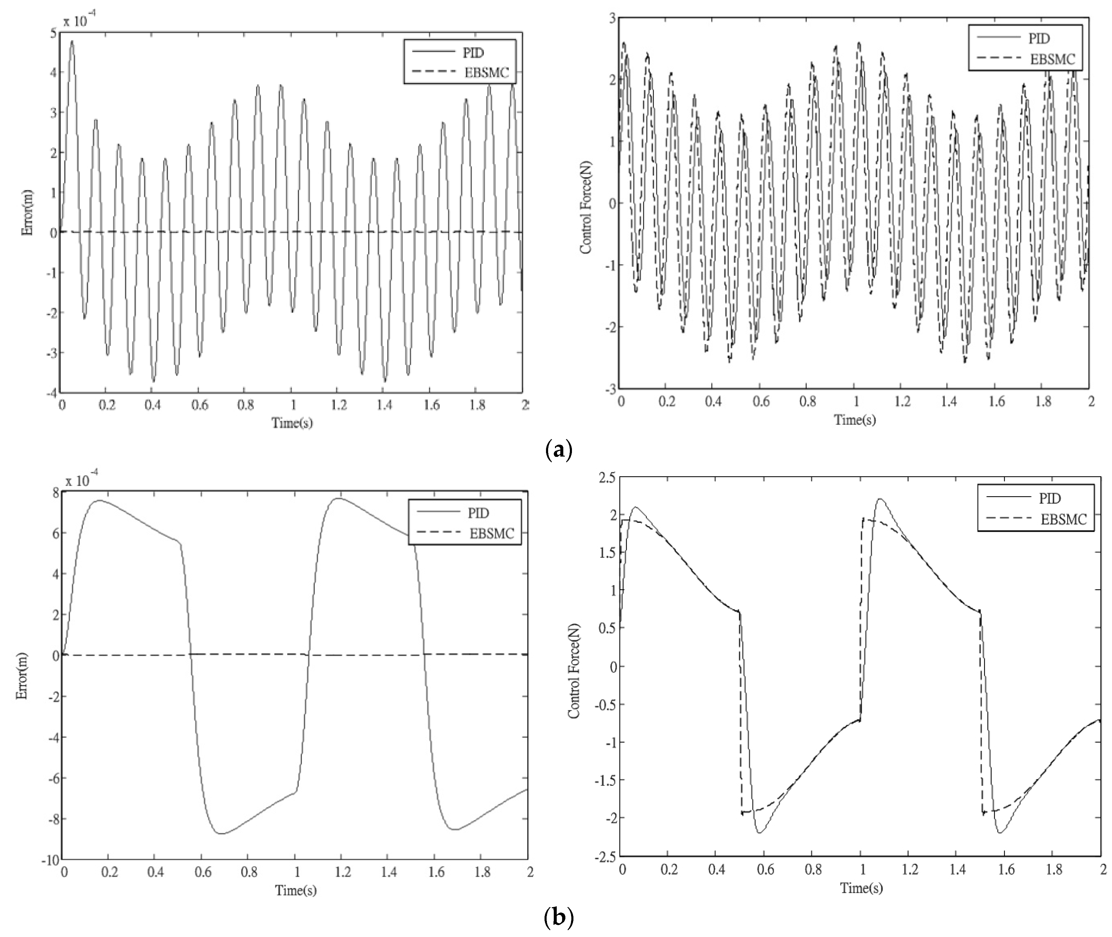
Comparing with the PID controller, to fairly address the main advantage of the proposed EBSMC, an equivalent control gain setting (that is K P = 1 + k 1 k 2 , K D = k 1 + k 2 and K I = w ) is applied. Moreover, in the following simulations, two cases are applied. Cases I and II are with the consideration of time varying external disturbance and nonlinear friction, respectively. The disturbance d = α sin ( 2 π f t ) is applied, where α = 2 and f = 10 Hz.
Figure 6a,b are the simulation results of Cases I and II, respectively. It is clear that the tracking performances of the proposed EBSMC for both cases is better than that by the PID controller. Detailed control performance comparisons are summarized in Table 2. Apparently, once the variation of the lumped perturbations is fast, the PID control performance will be degraded obviously. On the contrary, the EBSMC is able to achieve much better control precision even without the use of high gain control.

4. Experimental Study

In order to verify the feasibility of the proposed control scheme in practice, the following experimental study was conducted by an AC servomotor equipped with an encoder (10,000 counts/rev). The dynamics of the motor (i.e., J θ ¨ p = u F ) is similar to the system analyzed in Section 2, where the mass M ^ in (22) is replaced by the moment of inertia J ^ , and the tracking error is defined as e = θ d θ p . Apply the method presented in Section 4; the estimation nominal values of J ^ and σ ^ 2 in (22) are 6.0608 × 10 4 ( kg m A / N ) and 0.0018 ( kg m A / N / s ), respectively. An industrial computer equipped with a motion control card is used to implement the control algorithm, where the sampling rate is 500 Hz.
According to the analysis in Section 3, a precise estimation of the disturbance variation rate will be appreciated. However, due to the restriction of sensor resolution, it is hard to identify the parameters in the pre-sliding region (i.e., σ 0 , σ 1 ). Nevertheless, a suitable switching gain can reasonably be applied, such that the approaching condition is satisfied. In the experiments, both positioning control (i.e., x d is constant) and tracking control were performed to demonstrate the effectiveness of the proposed method. For positioning control, the reference position is 2 π rad (10,000 counts). The periodic reference command for tracking control is R [ 1 + sin ( 2 π f t + 1.5 π ) ] , where R = 2 π rad (10,000 counts) and f = 1 Hz. The control algorithm (22) was adopted for both positioning and tracking control. The value of w was altered to illustrate the resulting robustness. The values of control gains k 1 , k 2 and resulting performance indexes are listed in Table 3. Moreover, with the consideration of about 10% modeling errors and the selected gains, the robust stability (54) is feasible for w = 0 , where:
P = [ 116.7322 0.0308 0.0308 0.2588 ] , Q = [ 8.0203 0.0078 0.0078 0.0028 ] , ε = 11.6058
As a result, one can gradually increase the value of the robust gain step-by-step to achieve a satisfactory result without inducing system instability.
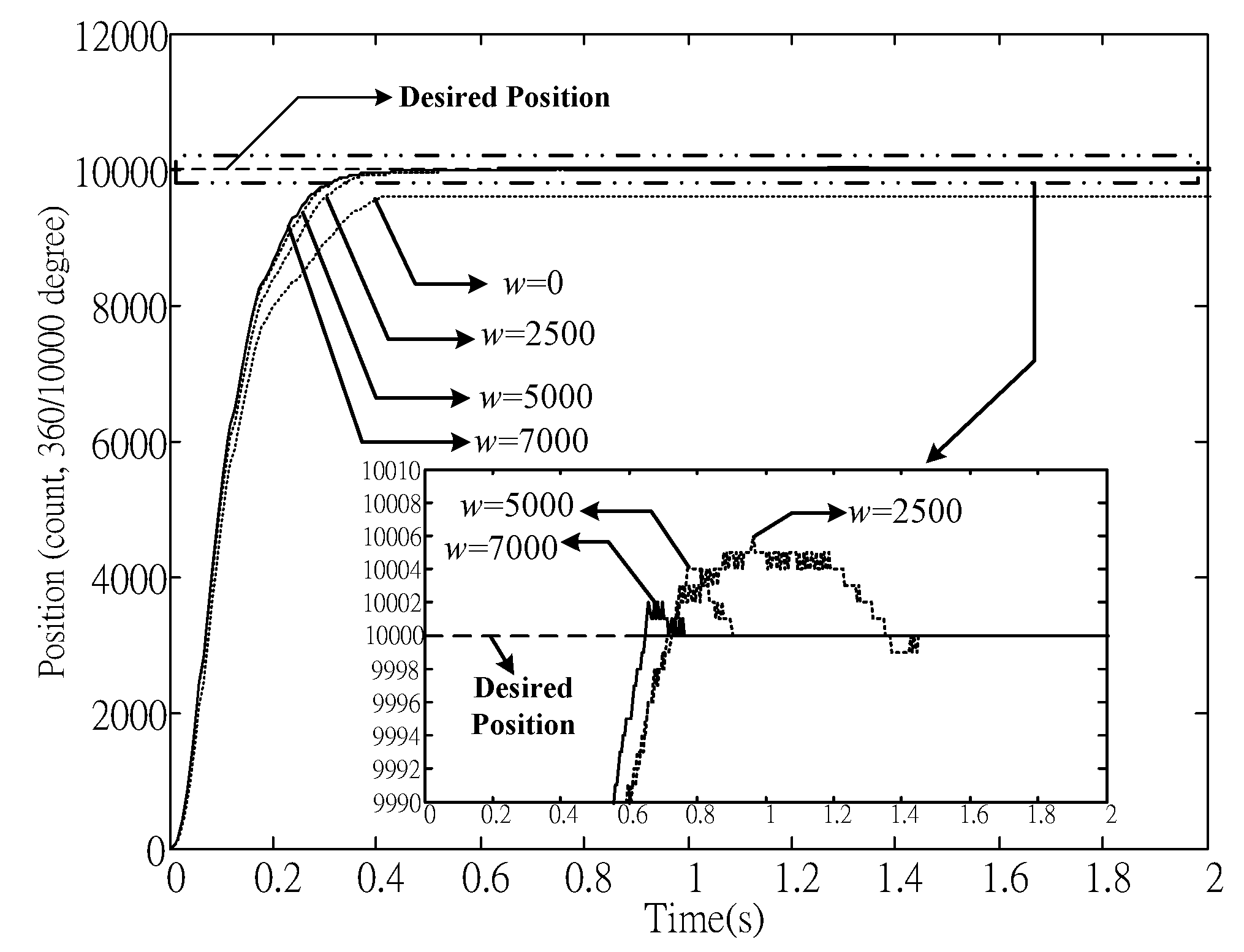
Figure 7 shows the positioning response, where the steady state error ( e s s ) caused by friction was eliminated via using gain w . In addition, a larger w also reduces overshoots and settling time t s s . Unlike the general PID controller, experiments showed that zero positioning error can be achieved without obvious overshoot. The control effort is shown in 
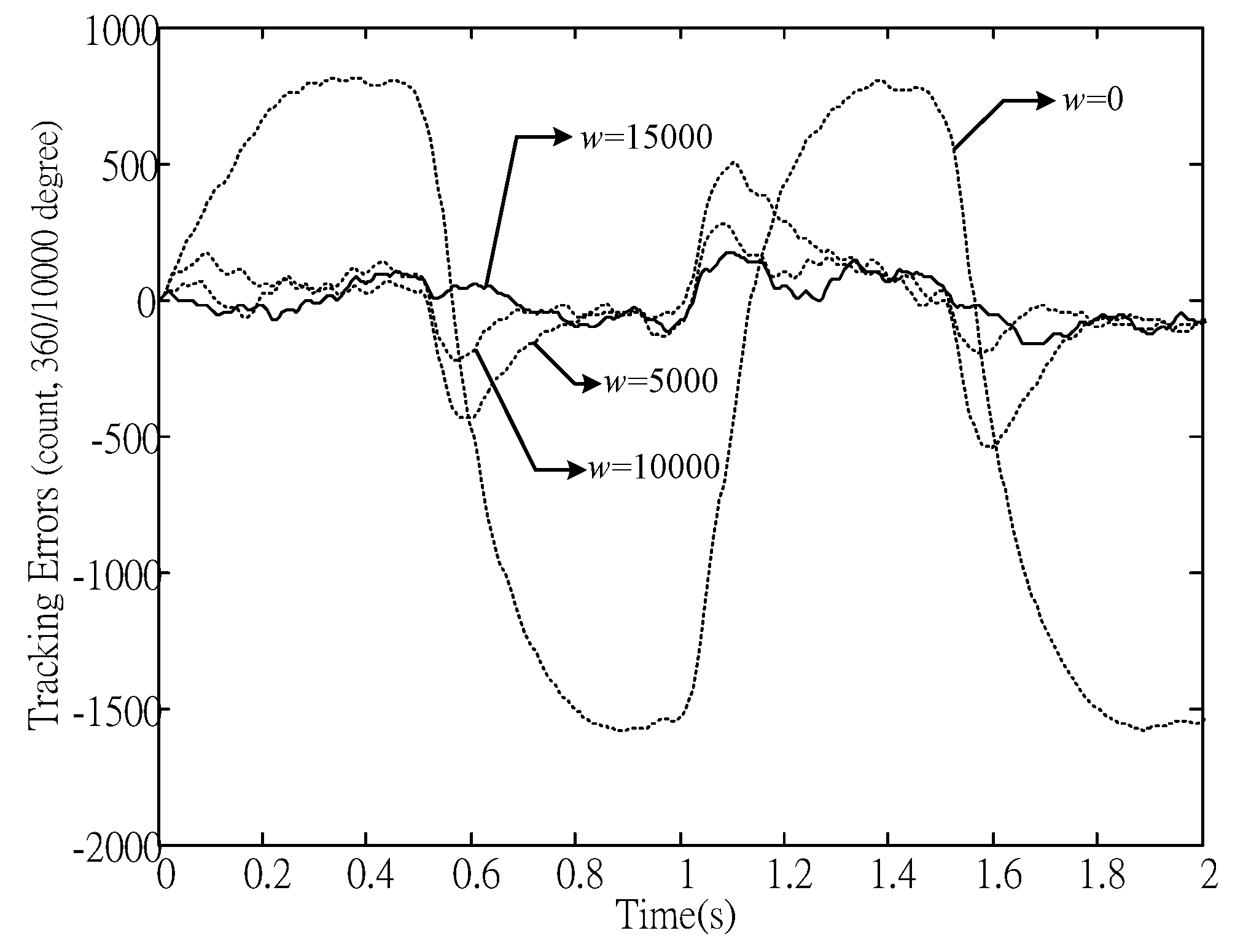
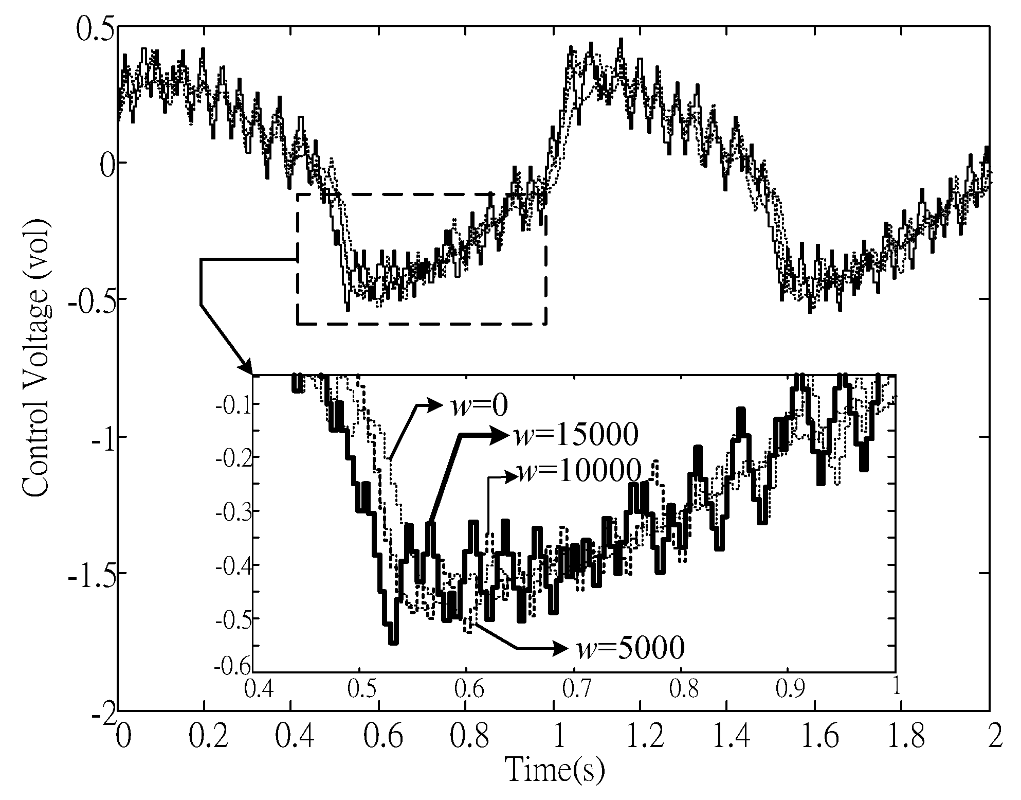
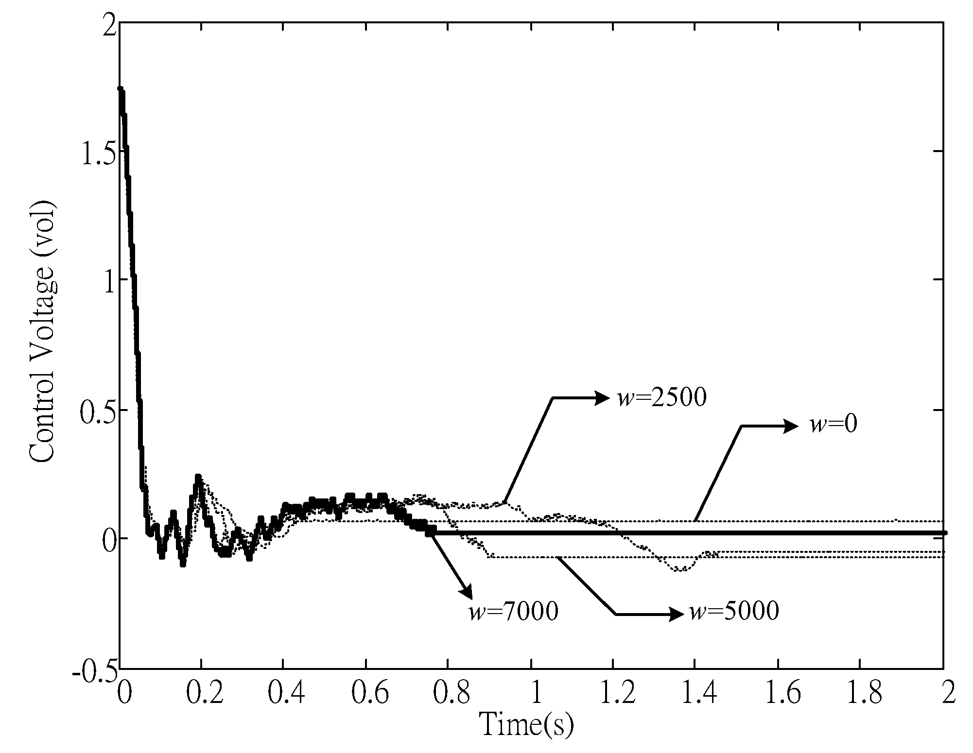
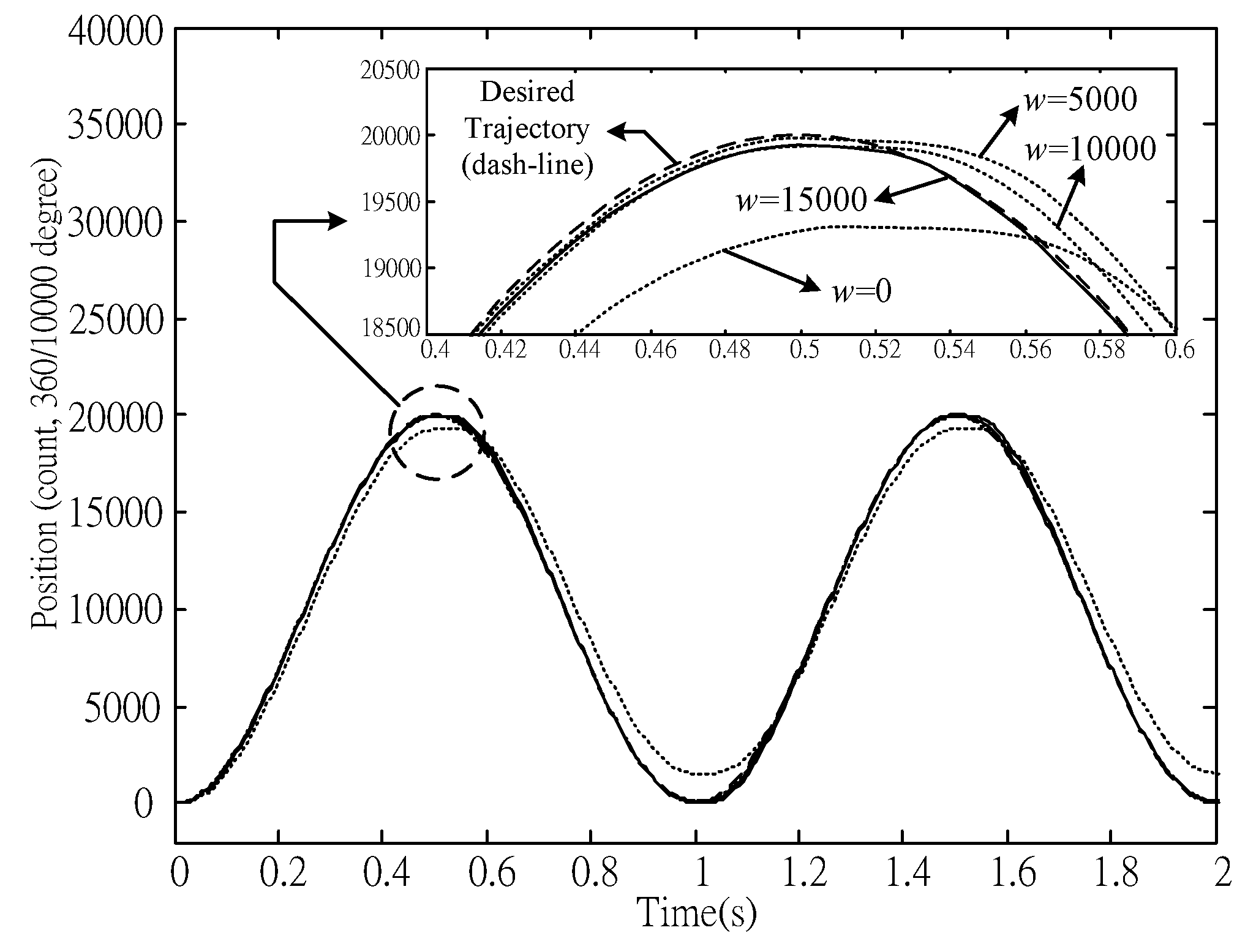
Figure 8, where the chattering phenomenon induced by the conventional sliding mode control was improved. System output responses, error response and control effort of tracking control with respect to w are shown in Figure 9, Figure 10 and Figure 11. The experimental results are consistent with (20) in that the larger the w, the larger the uncertain variation rates can be suppressed and, thereby, a better tracking performance can be obtained in the pre-sliding region (i.e., x ˙ p 0 ). All of the experiments show that the proposed method is capable of achieving good positioning/tracking performance, as well as avoiding significant control chattering.
In this study, we focus on motion control systems subject to nonlinear friction effects. To achieve good tracking precision, an EBSMC is proposed. However, the nonlinear friction effects must be continuous; that is, the upper bound of the time derivative of the friction should be finite. To satisfy this requirement, the LuGre friction model is considered. The LuGre model provides simple and continuous features for the friction forces, even when the velocity changes direction. As a result, the variation of the friction will be bounded. Otherwise, for discontinuous disturbances, both the conventional PID and the proposed EBSMC or other continuous control algorithms are not able to eliminate such fast switching perturbations.
Finally, for practical realization, the upper bound may not always be easy to identify. However, the robust gain w can be determined by increasing the value gradually. This feature has been verified through experiments.

5. Conclusions

To inherit the outstanding features, simple and straight forward stability proof, as well as attenuate the control discontinuity in the traditional SMC, an EBSMC design scheme is presented. For the developed control algorithm, the boundedness of the variation on the lumped perturbation is required. In the practical case, estimating the boundedness of the perturbation variation may not be an easy task. Therefore, based on the achievement of robust stability proven by LMIs, the proposed method allows the designer to apply it in a step by step tuning manner to pursue desired control performance without inducing unstable behavior. Based on the proposed method, the system stability is achieved via the backstepping design while the robustness against unknown perturbations is enhanced by a single robust gain. The proposed method did not use the additional friction model-based compensator or other disturbance observers, and therefore, the implementation effort is relatively low. Finally, simulations and experimental studies are addressed to verify the feasibility of the proposed method.

Acknowledgments

The work was supported by the Ministry of Science and Technology, Taiwan, under Grant Nos. MOST 105-2218-E-006-015 and MOST 105-2218-E-006-025.

Author Contributions

Li-Hsin Chen designed the controller and performed simulations. Chao-Chung Peng contributed to system stability analysis, servo motor identification procedure, experiments and wrote the article.

Conflicts of Interest

The authors declare no conflict of interest.

Appendix A

In this Appendix, a robust gain estimation is firstly introduced, and then, the robustness stability analysis for w = 0 is further addressed. The parameters of the motion tracking control system subjected to friction were listed in Table 1. According to the analysis in Section 2, the desired error dynamics can be guaranteed if the reaching condition (20) is satisfied. Therefore, it is important to estimate a suitable w for suppressing the disturbance effect on the control process. In the tracking task, most of the tracking errors are induced in the pre-sliding region, and it is reasonable to conclude that the variation rate of the disturbance in the pre-sliding region is larger than that in the sliding region. In other words, the reaching condition in the motion process is guaranteed if it can be satisfied in the pre-sliding region. For this reason, the variation rate of F B in the pre-sliding region should be estimated for determining a suitable w.
To fulfill the so-called approaching condition and attain the sliding condition, it has been shown in (20) that w > η should be satisfied. In other words, the derivation of the lumped perturbation needs to be bounded. In the following, the variation of the lumped perturbation is going to be addressed.
From (3), the deflection of the bristles is bounded, and its maximum value is κ s s = G ( x ˙ p ) sgn ( x ˙ p ) . Moreover, G ( x ˙ p ) is positive and bounded by f C / σ 0 G ( x ˙ p ) f S / σ 0 .
For x ˙ p 0 , the dynamic equation of the bristle can be represented as κ ˙ = x ˙ p x ˙ p G ( x ˙ p ) κ , and the following inequality can be obtained.
κ ˙ = x ˙ p x ˙ p G ( x ˙ p ) κ x ˙ p + x ˙ p G ( x ˙ p ) κ x ˙ p + x ˙ p f C σ 0 κ x ˙ p + x ˙ p f C σ 0 κ s s x ˙ p + x ˙ p f C σ 0 G ( x ˙ p ) x ˙ p + x ˙ p f C f S x ˙ p ( 1 + f S f C )
For x ˙ p 0 , x ¨ p 0 :
κ ¨ = x ¨ p x ¨ p G ( x ˙ p ) x ˙ p G ˙ ( x ˙ p ) G ( x ˙ p ) 2 κ x ˙ p G ( x ˙ p ) κ ˙ x ¨ p + x ¨ p G ( x ˙ p ) x ˙ p G ˙ ( x ˙ p ) G ( x ˙ p ) 2 κ + x ˙ p G ( x ˙ p ) κ ˙ x ¨ p + x ¨ p f S σ 0 x ˙ p { 1 σ 0 ( f S f C ) exp [ ( x ˙ p v S ) N ] [ N ( x ˙ p v S ) N 1 x ¨ p v S ] } ( f C / σ 0 ) 2 κ s s + x ˙ p ( f C / σ 0 ) κ ˙ x ¨ p + x ¨ p f S σ 0 + x ˙ p f S f C σ 0 N ( x ˙ p v S ) N 1 x ¨ p v S ( f C / σ 0 ) 2 κ s s + x ˙ p ( f C / σ 0 ) x ˙ p ( 1 + f S f C ) x ¨ p + x ¨ p f S σ 0 + x ˙ p f S f C σ 0 N ( x ˙ p v S ) N 1 x ¨ p v S ( f C / σ 0 ) 2 f S σ 0 + x ˙ p 2 ( f C / σ 0 ) ( 1 + f S f C ) x ¨ p + [ x ¨ p + x ˙ p ( 1 f C f S ) N ( x ˙ p v S ) N 1 x ¨ p v S ] ( f S f C ) 2 + x ˙ p 2 ( f C / σ 0 ) ( 1 + f S f C )
where G ˙ ( x ˙ p ) = N ( f S f C ) exp [ ( x ˙ p / v S ) N ] [ x ˙ p N 1 x ¨ p / v S N ] / σ 0 .
From (25) and (26), the maximum variation rate of the friction is:
F ˙ B = σ 0 κ ˙ + σ 1 κ ¨ σ 0 [ x ˙ p ( 1 + f S f C ) ] + σ 1 { x ¨ p + [ x ¨ p + x ˙ p ( 1 f C f S ) N ( x ˙ p v S ) N 1 x ¨ p v S ] ( f S f C ) 2 + x ˙ p 2 ( f C / σ 0 ) ( 1 + f S f C ) }
Based on the limitation of the possible maximum velocity and acceleration of the servo mechanism, (A3) is bounded, and therefore, exists. According to the desired motion trajectory, we can substitute its maximum velocity and maximum acceleration into (A3) to estimate the required gain w. However, for practical implementation, if the reference command is a sine wave as shown in Figure 1, the corresponding desired velocity in the pre-sliding region is not zero at the initial instant, such that if we adopt its value in (A3), it requires an extremely large gain w for achieving the approaching condition, but it may not be realizable in practice. Alternatively, a reference signal with zero velocity is preferred. Moreover, according to the friction model, Stribeck velocity determines which friction region occurs, so that v S and | x ¨ d | max are used for x ˙ p and x ¨ p , respectively, to obtain the maximum required w.
In Remark 2, the system stability is briefly addressed by means of BIBO for the critical condition w = 0. In the following, the closed-loop robust stability issue is going to be interpreted as a feasibility problem of a linear matrix inequality (LMI). According to (24), when applying zero robust gain, the sliding controller (22) turns into a PD control plus a feed-forward compensation, which leads to the following error dynamics:
e ˙ 2 = ( 1 + k 1 k 2 ) e 1 ( k 1 + k 2 ) e 2 + M ˜ M ( 1 + k 1 k 2 ) e 1 + M ˜ M ( k 1 + k 2 ) e 2 σ ˜ 2 M e 2 + σ ˜ 2 M x ˙ d + ( 1 M ˜ M ) x ¨ d + 1 M F B ( κ , κ ˙ ) + 1 M d
where M ˜ = M M ^ and σ ˜ 2 = σ 2 σ ^ 2 .
System (A4) can then be further represented by the following state space form:
e ˙ = ( A + Δ A ) e + D
where:
A = [ 0 1 ( 1 + k 1 k 2 ) ( k 1 + k 2 ) ] , Δ A = [ 0 0 M ˜ M ( 1 + k 1 k 2 ) M ˜ M ( k 1 + k 2 ) σ ˜ 2 M ] D = [ 0 σ ˜ 2 M x ˙ d + ( 1 M ˜ M ) x ¨ d + 1 M F B ( κ , κ ˙ ) + 1 M d ]
For (A5), consider a Lyapunov candidate as:
V e = e T Pe
where P T = P > 0 . Taking the time derivative of (A7) yields:
V ˙ e = e T ( A T P + PA + Δ A T P + P Δ A ) e + 2 e T PD
Since the last term in (A8) is bounded, the closed-loop system is said to be robust stable if the following inequality exists:
A T P + PA + Δ A T P + P Δ A + Q < 0
where Q T = Q > 0 .
According to the structure of Δ A , it can be factorized by:
Δ A = [ 0 0 ( 1 + k 1 k 2 ) ( k 1 + k 2 ) ] [ M ˜ M 0 0 M ˜ M σ ˜ 2 M ( k 1 + k 2 ) ] [ 1 0 0 1 ] = E F
and:
T < μ I
where μ is a known positive constant.
Furthermore, considering the following inequality:
Δ A T P + P Δ A = F T T E T P + PE F ε F T F + 1 ε μ PE E T P
where ε > 0 .
Based on (A12), (A9) is guaranteed as long as:
A T P + PA + ε F T F + 1 ε μ PE E T P + Q < 0
is attained.
As a result, it can be concluded that the robust stability can be guaranteed provided the following inequalities
[ A T P + PA + ε F T F + Q μ PE μ E T P ε ] < 0 P T = P > 0 , Q T = Q > 0 , ε > 0
are feasible.
Based on (A14), the Lyapunov function is re-written by:
V ˙ e e T Qe + 2 e T PD λ min ( Q ) e 2 + 2 λ max ( P ) e D λ min ( Q ) e ( e 2 λ max ( P ) λ min ( Q ) D )
which indicates that:
e Ω : = 2 λ max ( P ) λ min ( Q ) D
eventually. As a result, a robust stability can be guaranteed, even when w = 0.

References

  1. Marquez, H.J. Nonlinear Control Systems Analysis and Design; John Wiley & Sons: Hoboken, NJ, USA, 2003; pp. 137–148. [Google Scholar]
  2. Tan, Y.; Chang, J.; Tan, H.; Hu, J. Integral backstepping control and experimental implementation for motion system. In Proceedings of the 2000 IEEE International Conference on Control Applications, Anchorage, AK, USA, 25–27 September 2000; pp. 367–372.
  3. Yu, J.; Chang, J. A new adaptive backstepping control algorithm for motion control systems. In Proceedings of the 2002 Power Conversion Conference, PCC-Osaka 2002, Osaka, Japan, 2–5 April 2002; Volume 1, pp. 206–210.
  4. Benaskeur, A.; Desbiens, A. Backstepping-based adaptive PID control. IEE Proc. Control Theory Appl. 2002, 149, 54–59. [Google Scholar] [CrossRef]
  5. Lin, F.-J.; Shen, P.-H.; Hsu, S.-P. Adaptive backstepping sliding mode control for linear induction motor drive. Proc. IEE Electr. Power Appl. 2002, 149, 184–194. [Google Scholar] [CrossRef]
  6. Stotsky, A.; Hedrick, J.; Yip, P. The use of sliding modes to simplify the backstepping control method. In Proceedings of the American Control Conference, Albuquerque, NM, USA, 6 June 1997; pp. 1703–1708.
  7. Kwan, C.M.; Lewis, F.L. Robust backstepping control of induction motors using neural networks. IEEE Trans. Neural Netw. 2000, 11, 1178–1187. [Google Scholar] [CrossRef] [PubMed]
  8. Kwan, C.M.; Lewis, F.L. Robust backstepping control of nonlinear systems using neural networks. IEEE Trans. Syst. Man Cybern. A Syst. Hum. 2000, 30, 753–766. [Google Scholar] [CrossRef]
  9. Hua, C.; Guan, X.; Shi, P. Robust backstepping control for a class of time delayed systems. IEEE Trans. Autom. Control 2005, 50, 894–899. [Google Scholar]
  10. Koshkouei, A.J.; Zinober, A.S.I. Adaptive backstepping control of nonlinear systems with unmatched uncertainty. In Proceedings of the 39th IEEE Conference on Decision and Control, Atlanta, GA, USA, 12–15 December 2000; Volume 5, pp. 4765–4770.
  11. Zhou, J.; Wen, C.; Zhang, Y. Adaptive backstepping control of a class of uncertain nonlinear systems with unknown backlash-like hysteresis. IEEE Trans. Autom. Control 2004, 49, 1751–1759. [Google Scholar] [CrossRef]
  12. Arcak, M.; Seron, M.; Braslavsky, J.; Kokotovic, P. Robustification of backstepping against input unmodeled dynamics. IEEE Trans. Autom. Control 2000, 45, 1358–1363. [Google Scholar] [CrossRef]
  13. Chen, C.L.; Yau, H.T.; Peng, C.C. Design of Extended Backstepping Sliding mode Controller for Uncertain Chaotic Systems. Int. J. Nonlinear Sci. Numer. 2007, 8, 137–146. [Google Scholar] [CrossRef]
  14. Chen, C.L.; Peng, C.C.; Yau, H.T. High-Order Sliding Mode Controller with Backstepping Design for Aeroelastic Systems. Commun. Nonlinear Sci. 2011, 17, 1813–1823. [Google Scholar] [CrossRef]
  15. Peng, C.C.; Hsue, A.W.; Chen, C.L. Variable structure based robust backstepping controller design for nonlinear systems. Nonlinear Dyn. 2011, 63, 253–262. [Google Scholar] [CrossRef]
  16. Peng, C.C.; Su, Y.T. Sliding Controller Design for Servo Drive Systems subject to Mechanical and Electrical Perturbations. In Proceedings of the 2016 IEEE International Conference on Industrial Technology (ICIT), Taipei, Taiwan, 14–17 March 2016.
  17. Chen, C.L.; Lin, K.C.; Hsieh, C. Presliding friction mode: Modelling and experimental study with a ball-screw-driven set-up. Math. Comput. Model. Dyn. Syst. 2005, 11, 397–410. [Google Scholar] [CrossRef]
  18. Tan, Y.; Chang, J.; Tan, H. Adaptive backstepping control and friction compensation for AC servo with inertia and load uncertainties. IEEE Trans. Ind. Electron. 2003, 50, 944–952. [Google Scholar]
  19. Lee, H.S.; Tomizuka, M. Robust motion controller design for high-accuracy positioning systems. IEEE Trans. Ind. Electron. 1996, 43, 48–55. [Google Scholar]
  20. Kim, B.K.; Chung, W.K. Performance tuning of robust motion controllers for high-accuracy positioning systems. IEEE-ASME Trans. Mechatron. 2002, 7, 500–514. [Google Scholar] [CrossRef]
  21. Liu, Z.Z.; LiLuo, F.; Rahman, M.A. Robust and precision motion control system of linear-motor direct drive for high-speed X-Y table positioning mechanism. IEEE Trans. Ind. Electron. 2005, 52, 1357–1363. [Google Scholar] [CrossRef]
  22. Lin, C.J.; Li, M.J.; Liu, K.R. Tracking control of an Ultrasonic linear motor actuated stage using a sliding-mode controller with friction compensation. Smart Sci. 2015, 3, 35–39. [Google Scholar] [CrossRef]
  23. Cho, G.R.; Park, S.H.; Chang, P.H.; Jin, M. Robust tracking under nonlinear friction using time delay control with internal model. IEEE Trans. Control Syst. Technol. 2009, 17, 1406–1414. [Google Scholar]
  24. Jin, Y.; Chang, P.H.; Jin, M.; Gweon, D.G. Stability guaranteed time delay control of manipulators using nonlinear damping and terminal sliding mode. IEEE Trans. Ind. Electron. 2013, 60, 3304–3317. [Google Scholar] [CrossRef]
  25. Hsieh, C.; Pan, Y.C. Dynamic behavior and modelling of the pre-sliding static friction. Wear 2000, 242, 1–17. [Google Scholar] [CrossRef]
  26. Canudas de Wit, C.; Olsson, H.; Astrom, K.J.; Lischinsky, P. A new model for control of systems with friction. IEEE Trans. Autom. Control 1995, 40, 419–425. [Google Scholar] [CrossRef]
  27. Xie, W.-F. Sliding-Mode-Observer-Based Adaptive Control for Servo Actuator with Friction. IEEE Trans. Ind. Electron. 2007, 54, 1517–1527. [Google Scholar] [CrossRef]
  28. Yao, B. Integrated Direct/Indirect Adaptive Robust Control of SISO Nonlinear Systems in Semi-Strict Feedback Form. In Proceedings of the American Control Conference, Denver, CO, USA, 4–6 June 2003.
  29. Chen, C.L.; Xu, R.L. Tracking control of robot manipulator using sliding mode controller with performance robustness. J. Dyn. Syst. Meas. Control Trans. ASME 1999, 121, 64–70. [Google Scholar] [CrossRef]
  30. Kuo, C.T.; Lee, C.H. Network-based type-2 fuzzy system with water flow like algorithm for system identification and signal processing. Smart Sci. 2015, 3, 21–34. [Google Scholar] [CrossRef]
Figure 1. Reference command x d 1 .
Applsci 07 00220 g001
Figure 2. Reference command x d 2 .
Applsci 07 00220 g002
Figure 3. Tracking error comparison.
Applsci 07 00220 g003
Figure 4. Control force comparison.
Applsci 07 00220 g004
Figure 5. Sliding surface comparison.
Applsci 07 00220 g005
Figure 6. Performance comparisons between PID control and extended backstepping sliding mode control (EBSMC). (a) system subject to time varying external disturbance; (b) system subject to nonlinear friction.
Applsci 07 00220 g006
Figure 7. Experimental result of positioning control.
Applsci 07 00220 g007
Figure 8. Positioning control effort.
Applsci 07 00220 g008
Figure 9. Experiment result of tracking control.
Applsci 07 00220 g009
Figure 10. Comparison of tracking error.
Applsci 07 00220 g010
Figure 11. Tracking control effort.
Applsci 07 00220 g011
Table 1. Parameter values used for numerical study.
ParameterValueUnit
M ( M ^ )1.5 (1.2)(kg)
σ 0 105(N/m)
σ 1 105/2(Ns/m)
σ 2 ( σ ^ 2 )2.5 (2.0)(Ns/m)
f C 1.3(N)
f S 1.5(N)
v S 0.001(m/s)
R 0.01(m)
f 1(Hz)
N 2 ---
k 1 30---
k 2 50---
w 603---
Table 2. Numerical control performance comparison.
Controller e max e r m s e
Case I.
External Disturbance
PID4.7691 × 10−42.1244 × 10−40.0601
K P = 1501 , K D = 80 , K I = 603
EBSMC2.0468 × 10−71.1448 × 10−73.2380 × 10−5
k 1 = 30 , k 2 = 50 , w = 603
Case II.
Nonlinear Friction
PID7.6552 × 10−46.7840 × 10−40.1919
K P = 1501 , K D = 80 , K I = 603
EBSMC1.3089 × 10−61.1904 × 10−63.3669 × 10−4
k 1 = 30 , k 2 = 50 , w = 603
Table 3. Control gains setting in experiments.
Control TaskControl Gains | e s s | (Counts)Overshoot (Counts) t s s (s)
Positioning Controlk1 = 15, k2 = 30, w = 0295-0.75
k1 = 15, k2 = 30, w = 2500061.45
k1 = 15, k2 = 30, w = 5000040.905
k1 = 15, k2 = 30, w = 7000020.765
Control TaskControl GainsMaximum Tracking Error | e | max (counts)
Tracking Controlk1 = 15, k2 = 30, w = 01584
k1 = 15, k2 = 30, w = 5000544
k1 = 15, k2 = 30, w = 10,000280
k1 = 15, k2 = 30, w = 15,000173

