Improving Multi-Instance Multi-Label Learning by Extreme Learning Machine

Abstract

Multi-instance multi-label learning is a learning framework, where every object is represented by a bag of instances and associated with multiple labels simultaneously. The existing degeneration strategy-based methods often suffer from some common drawbacks: (1) the user-specific parameter for the number of clusters may incur the effective problem; (2) SVM may bring a high computational cost when utilized as the classifier builder. In this paper, we propose an algorithm, namely multi-instance multi-label (MIML)-extreme learning machine (ELM), to address the problems. To our best knowledge, we are the first to utilize ELM in the MIML problem and to conduct the comparison of ELM and SVM on MIML. Extensive experiments have been conducted on real datasets and synthetic datasets. The results show that MIMLELM tends to achieve better generalization performance at a higher learning speed.

1. Introduction

When utilizing machine learning to solve practical problems, we often consider an object as a feature vector. Then, we get an instance of the object. Further, associating the instance with a specific class label of the object, we obtain an example. Given a large collection of examples, the task is to get a function mapping from the instance space to the label space. We expect that the learned function can predict the labels of unseen instances correctly. However, in some applications, a real-world object is often ambiguous, which consists of multiple instances and corresponds to multiple different labels simultaneously.

For example, an image usually contains multiple patches each represented by an instance, while in image classification, such an image can belong to several classes simultaneously, e.g., an image can belong to mountains, as well as Africa [1]; another example is text categorization [1], where a document usually contains multiple sections each of which can be represented as an instance, and the document can be regarded as belonging to different categories if it were viewed from different aspects, e.g., a document can be categorized as a scientific novel, Jules Verne’s writing or even books on traveling. The MIML (Multi-instance Multi-label) problem also arises in the protein function prediction task [2]. A domain is a distinct functional and structural unit of a protein. A multi-functional protein often consists of several domains, each fulfilling its own function independently. Taking a protein as an object, a domain as an instance and each biological function as a label, the protein function prediction problem exactly matches the MIML learning task.

In this context, multi-instance multi-label learning was proposed [1]. Similar to the other two multi-learning frameworks, i.e., multi-instance learning (MIL) [3] and multi-label learning (MLL) [4], the MIML learning framework also results from the ambiguity in representing the real-world objects. Differently, more difficult than two other multi-learning frameworks, MIML studies the ambiguity in terms of both the input space (i.e., instance space) and the output space (i.e., label space), while MIL just studies the ambiguity in the input space and MLL just the ambiguity in the output space, respectively. In [1], Zhou et al. proposed a degeneration strategy-based framework for MIML, which consists of two phases. First, the MIML problem is degenerated into the single-instance multi-label (SIML) problem through a specific clustering process; second, the SIML problem is decomposed into a multiple independent binary classification (i.e., single-instance single-label) problem using Support Vector Machine (SVM) as the classifiers builder. This two-phase framework has been successfully applied to many real-world applications and has been shown to be effective [5]. However, it could be further improved if the following drawbacks are tackled. On one hand, the clustering process in the first phase requires a user-specific parameter for the number of clusters. Unfortunately, it is often difficult to determine the correct number of clusters in advance. The incorrect number of clusters may affect the accuracy of the learning algorithm; on the other hand, SIML is degenerated into single-instance single-label learning (SISL) (i.e., single instance, single label) in the second phase, as this will increase the volume of data to be handled and thus burden the classifier building. Utilizing SVM as the classifier builder in this phase may suffer from a high computational cost and require a number of parameters to be optimized.

In this paper, we propose to enhance the two-phase framework by tackling the two above issues and make the following contributions: (1) We utilize extreme learning machine (ELM) [6] instead of SVM to improve the efficiency of the two-phase framework. To our best knowledge, we are the first to utilize ELM in the MIML problem and to conduct the comparison of ELM and SVM on MIML. (2) We design a method of theoretical guarantee to determine the number of clusters automatically while incorporating it into the improved two-phase framework for effectiveness.

The remainder of this paper is organized as follows. In Section 2, we give a brief introduction to MIML and ELM. Section 3 details the improvements of the two-phase framework. Experimental analysis is given in Section 4. Finally, Section 5 concludes this paper.

2. The Preliminaries

This research is related to some previous work on MIML learning and ELM. In what follows, we briefly review some preliminaries of the two related works in Section 2.1 and Section 2.2, respectively.

2.1. Multi-Instance Multi-Label Learning

In traditional supervised learning, the relationships between an object and its description and its label are always a one-to-one correspondence. That is, an object is represented by a single instance and associated with a single class label. In this sense, we refer to it as single-instance single-label learning (SISL). Formally, let X be the instance space (or say, feature space) and Y the set of class labels. The goal of SISL is to learn a function $f_{SISL}$: X→Y from a given dataset $\{(x_1,y_1),(x_2,y_2),\dots ,(x_m,y_m)\}$, where $x_i$∈X is an instance and $y_i$∈Y is the label of $x_i$. This formalization is prevailing and successful. However, as mentioned in Section 1, many real-world objects are complicated and ambiguous in their semantics. Representing these ambiguous objects with SISL may lose some important information and make the learning task problematic [1]. Thus, many real-world complicated objects do not fit in this framework well.

In order to deal with this problem, several multi-learning frameworks have been proposed, e.g., multi-instance learning (MIL), multi-label learning (MLL) and multi-instance multi-label Learning (MIML). MIL studies the problem where a real-world object described by a number of instances is associated with a single class label. The training set for MIL is composed of many bags each containing multiple instances. In particular, a bag is labeled positively if it contains at least one positive instance and negatively otherwise. The goal is to label unseen bags correctly. Note that although the training bags are labeled, the labels of their instances are unknown. This learning framework was formalized by Dietterich et al. [3] when they were investigating drug activity prediction. Formally, let X be the instance space (or say, feature space) and Y the set of class labels. The task of MIL is to learn a function $f_{MIL}$$:2^X$→$\{-1,+1\}$ from a given dataset $\{(X_1,y_1),(X_2,y_2),\dots ,(X_m,y_m)\}$, where $X_i$⊆X is a set of instances $\{x_1^{(i)},x_2^{(i)},\dots ,x_{n_i}^{(i)}\}$, $x_j^{(i)}$∈X$(j=1,2,\dots ,n_i)$, and $y_i$∈$\{-1,+1\}$ is the label of $X_i$. Multi-instance learning techniques have been successfully applied to diverse applications, including image categorization [7,8], image retrieval [9,10], text categorization [11,12], web mining [13], spam detection [14], face detection [15], computer-aided medical diagnosis [16], etc. Differently, MLL studies the problem where a real-world object is described by one instance, but associated with a number of class labels. The goal is to learn a function $f_{MLL}$$:X$→$2^Y$ from a given dataset $\{(x_1,Y_1),(x_2,Y_2)$, $\dots ,(x_m,Y_m)\}$, where $x_i$∈X is an instance and $Y_i$⊆Y a set of labels $\{y_1^{(i)},y_2^{(i)},\dots ,y_{l_i}^{(i)}\}$, $y_k^{(i)}$∈Y$(k=1,2,\dots ,l_i)$. The existing work of MLL falls into two major categories. One attempts to divide multi-label learning to a number of two class classification problems [17,18] or to transform it into a label ranking problem [19,20]; the other tries to exploit the correlation between the labels [21,22]. MLL has been found useful in many tasks, such as text categorization [23], scene classification [24], image and video annotation [25,26], bioinformatics [27,28] and even association rule mining [29,30].

MIML is a generalization of traditional supervised learning, multi-instance learning and multi-label learning, where a real-world object may be associated with a number of instances and a number of labels simultaneously. In some cases, transforming single-instance multi-label objects to MIML objects for learning may be beneficial. Before the explanation, we first introduce how to perform such a transformation. Let S = $\{({\mathbf{x}}_1,Y_1),({\mathbf{x}}_2,Y_2)$, $\dots ,({\mathbf{x}}_m,Y_m)\}$ be the dataset, where ${\mathbf{x}}_i$∈X is an instance and $Y_i$⊆Y a set of labels $\{y_1^{(i)},y_2^{(i)},\dots ,y_{l_i}^{(i)}\}$, $y_k^{(i)}$∈Y$(k=1,2,\dots ,l_i)$. We can first obtain a vector ${\mathbf{v}}_l$ for each class label l∈Y by averaging all of the training instances of label l, i.e., ${\mathbf{v}}_l$ = $\frac{1}{|S_l|}\sum _{{\mathbf{x}}_i\in S_l}{\mathbf{x}}_i$, where $S_l$ is the set of all of the training instances ${\mathbf{x}}_i$ of label l. Then, each instance can be transformed into a bag, $B_i$, of $\left|Y\right|$ instances by computing $B_i$ = $\{{\mathbf{x}}_i$ − ${\mathbf{v}}_l|l$∈$Y\}$. As such, the single-instance multi-label dataset S is transformed into an MIML dataset $S^{\prime }$ = $\{(B_1,Y_1),(B_2,Y_2)$, $\dots ,(B_m,Y_m)\}$. The benefits of such a transformation are intuitive. First, for an object associated with multiple class labels, if it is described by only a single instance, the information corresponding to these labels is mixed and thus difficult to learn. However, by breaking the single-instance into a number of instances, each corresponding to one label, the structure information collapsed in the single-instance representation may become easier to exploit. Second, for each label, the number of training instances can be significantly increased. Moreover, when representing the multi-label object using a set of instances, the relation between the input patterns and the semantic meanings may become more easily discoverable. In some cases, understanding why a particular object has a certain class label is even more important than simply making an accurate prediction while MIML offers a possibility for this purpose. For example, using MIML, we may discover that one object has label $l_1$ because it contains $instanc{e}_n$; it has label $l_k$ because it contains $instanc{e}_i$; while the occurrence of both $instanc{e}_1$ and $instanc{e}_i$ triggers label $l_j$. Formally, the task of MIML is to learn a function $f_{MIML}$$:2^X\to 2^Y$ from a given dataset $\{(X_1,Y_1),(X_2,Y_2),\dots ,(X_m,Y_m)\}$, where $X_i$⊆X is a set of instances $\{x_1^{(i)},x_2^{(i)},\dots ,x_{n_i}^{(i)}\}$, $x_j^{(i)}$∈X$(j=1,2,\dots ,n_i)$ and $Y_i$⊆Y is a set of labels $\{y_1^{(i)},y_2^{(i)},\dots ,y_{l_i}^{(i)}\}$, $y_k^{(i)}$∈X$(k=1,2,\dots ,l_i)$. Figure 1 illustrates the relationship among the four learning frameworks mentioned above.

2.2. A Brief Introduction to ELM

Extreme learning machine (ELM) is a generalized single hidden-layer feedforward network. In ELM, the hidden-layer node parameter is mathematically calculated instead of being iteratively tuned; thus, it provides good generalization performance at thousands of times faster speed than traditional popular learning algorithms for feedforward neural networks [31].

As a powerful classification model, ELM has been widely applied in many fields. For example, in [32], ELM was applied for plain text classification by using the one-against-one (OAO) and one-against-all (OAA) decomposition scheme. In [31], an ELM-based XML document classification framework was proposed to improve classification accuracy by exploiting two different voting strategies. A protein secondary prediction framework based on ELM was proposed in [33] to provide good performance at extremely high speed. The work in [34] implemented the protein-protein interaction prediction on multi-chain sets and on single-chain sets using ELM and SVM for a comparable study. In both cases, ELM tends to obtain higher recall values than SVM and shows a remarkable advantage in computational speed. The work in [35] evaluated the multi-category classification performance of ELM on three microarray datasets. The results indicate that ELM produces comparable or better classification accuracies with reduced training time and implementation complexity compared to artificial neural network methods and support vector machine methods. In [36], the use of ELM for multiresolution access of terrain height information was proposed. The optimization method-based ELM for classification was studied in [37].

ELM not only tends to reach the smallest training error, but also the smallest norm of weights [6]. Given a training set D = $\left\{({\mathbf{x}}_i,{\mathbf{t}}_i)\right|{\mathbf{x}}_i\in {\mathbf{R}}^n,{\mathbf{t}}_i\in {\mathbf{R}}^m,i=1,\dots ,N\}$, activation function $g(x)$ and hidden node number L, the pseudocode of ELM is given in Algorithm 1. More detailed introductions to ELM can be found in a series of published literature [6,37,38].

3. The Proposed Approach MIMLELM

MIMLSVM is a representative two-phase MIML algorithm successfully applied in many real-world tasks [2]. It was first proposed by Zhou et al. in [1] and recently improved by Li et al., in [5]. MIMLSVM solves the MIML problem by first degenerating it into single-instance multi-label problems through a specific clustering process and then decomposing the learning of multiple labels into a series of binary classification tasks using SVM. However, as mentioned, MIMLSVM may suffer from some drawbacks in either of the two phases. For example, in the first phase, the user-specific parameter for the number of clusters may incur the effective problem; in the second phase, utilizing SVM as the classifiers builder may bring high computational cost and require a great number of parameters to be optimized.

In this paper, we present another algorithm, namely MIMLELM, to make MIMLSVM more efficient and effective. In this proposed method: (1) We utilize ELM instead of SVM to improve the efficiency of the two-phase framework. To our best knowledge, we are the first to utilize ELM in the MIML problem and to conduct the comparison of ELM and SVM on MIML. (2) We develop a method of theoretical guarantee to determine the number of clusters automatically, so that the transformation from MIML to SIML is more effective. (3) We exploit a genetic algorithm-based ELM ensemble to further improve the prediction performance.

The MIMLELM algorithm is outlined in Algorithm 2. It consists of four major elements: (1) determination the number of clusters (Line 2); (2) transformation from MIML to SIML (Lines 3–12); (3) transformation from SIML to SISL (Lines 13–17); (4) multi-label learning based on ELM (Lines 18–19). In what follows, we will detail the four elements in Section 3.1, Section 3.2, Section 3.3 and Section 3.4, respectively.

3.1. Determination of the Number of Clusters

The primary important task for MIMLELM is to transform MIML into SIML. Unlike MIMLSVM, which performs the transformation through a clustering process with a user-specified parameter for the number of clusters, we utilize AIC [39], a model selection criterion, to automatically determine the number of clusters.

$AIC$ is founded on information theory. It offers a relative estimation of the information lost when a given model is used to represent the process that generates the data. For any statistical model, the general form of $AIC$ is $AIC$ = $-2ln(L)$+$2K$, where L is the maximized value of the likelihood function for the model and K is the number of parameters in the model. Given a set of candidate models, the one of the minimum $AIC$ value is preferred [39].

Let $M_k$ be the model of the clustering result with k clusters $C_1$, $C_2$, …, $C_k$, where the number of samples in $C_i$ is $m_i$. $X_i$ denotes a random variable indicating the $PD$ value between any pair of micro-clusters in $C_i$. Then, under a general assumption commonly used in the clustering community, $X_i$ follows a Gaussian distribution with (${\mu }_i,{\sigma }_i^2$), where ${\mu }_i$ is the expected $PD$ value between any pair of micro-clusters in $C_i$, and ${\sigma }_i^2$ is the corresponding variance. That is, the probability density of $X_i$ is:

$$p(X_i)=\frac{m_i}{m}·\frac{1}{\sqrt{2\pi }{\sigma }_i}exp(-\frac{1}{2{\sigma }_i^2}{(X_i-{\mu }_i)}^2)$$

(1)

Let $x_{i_j}$ (1≤j≤$C_{m_i}^2$) be an observation of $X_i$; the corresponding log-likelihood w.r.t the data in $C_i$ is:

$$\begin{array}{cc}& lnL(C_i|{\mu }_i,{\sigma }_i)=ln{\displaystyle \prod _{j=1}^{C_{m_i}^2}}p(X_i=x_{i_j})={\displaystyle \sum _{j=1}^{C_{m_i}^2}}(ln\frac{1}{\sqrt{2\pi }{\sigma }_i}-\frac{1}{2{\sigma }_i^2}{(x_{i_j}-{\mu }_i)}^2+ln\frac{m_i}{m})\hfill \end{array}$$

(2)

Since the fact that the log-likelihood for all clusters is the sum of the log-likelihood of the individual clusters, the log-likelihood of the data w.r.t $M_k$ is:

$$\begin{array}{cc}& lnL(M_k|{\mu }_1,{\mu }_2,\dots ,{\mu }_k,{\sigma }_1,{\sigma }_2,\dots ,{\sigma }_k)={\displaystyle \sum _{i=1}^k}lnL(C_i|{\mu }_i,{\sigma }_i)={\displaystyle \sum _{i=1}^k}{\displaystyle \sum _{j=1}^{C_{m_i}^2}}(ln\frac{1}{\sqrt{2\pi }{\sigma }_i}-\frac{1}{2{\sigma }_i^2}{(x_{i_j}-{\mu }_i)}^2+ln\frac{m_i}{m})\hfill \end{array}$$

(3)

Further, take the MLE (maximum likelihood estimate) of ${\sigma }_i^2$, i.e.: $\widehat{{\sigma }_i^2}$ = $\frac{1}{C_{m_i}^2}{\displaystyle \sum _{j=1}^{C_{m_i}^2}}{(x_{i_j}-{\mu }_i)}^2$, into Equation (3); we obtain that:

$$\begin{array}{cc}& lnL(M_k|{\mu }_1,{\mu }_2,\dots ,{\mu }_k,{\sigma }_1,{\sigma }_2,\dots ,{\sigma }_k)=-\frac{{\displaystyle \sum _{i=1}^k}{C}_{m_i}^2}{2}ln(2\pi )\hfill \\ & -\frac{{\displaystyle \sum _{i=1}^k}{C}_{m_i}^{2}ln(\widehat{{\sigma }_i^2})}{2}-\frac{{\displaystyle \sum _{i=1}^k}{C}_{m_i}^2}{2}+{\displaystyle \sum _{i=1}^k}{C}_{m_i}^{2}ln{m}_i-lnm{\displaystyle \sum _{i=1}^k}{C}_{m_i}^2\hfill \end{array}$$

(4)

Finally, in our case, the number of independent parameters K is $2k$. Thus, $AIC$ of the model $M_k$ is:

$$\begin{array}{cc}& AI{C}_{M_k}=ln(2\pi m^{2}e){\displaystyle \sum _{i=1}^k}{C}_{m_i}^2+{\displaystyle \sum _{i=1}^k}{C}_{m_i}^{2}ln(\widehat{{\sigma }_i^2})-2{\displaystyle \sum _{i=1}^k}{C}_{m_i}^{2}ln{m}_i+4k\hfill \end{array}$$

(5)

3.2. Transformation from MIML to SIML

With the number of clusters computed, we start to transform the MIML learning task, i.e., learning a function $f_{MIML}$$:2^X$→$2^Y$, to a multi-label learning task, i.e., learning a function $f_{MLL}$$:Z$→$2^Y$.

Given an MIML training example, the goal of this step is to get a mapping function $z_i$ = $\varphi (X_i)$, where ϕ$:2^x$→Z, such that for any $z_i$∈Z, $f_{MLL}(z_i)$ = $f_{MIML}(X_i)$ if $z_i$ = $\varphi (X_i)$. As such, the proper labels of a new example $X_k$ can be determined according to $Y_k$ = $f_{MLL}(\varphi (X_k))$. Since the proper number of clusters has been automatically determined in Section 3.1, we implement the mapping function $\varphi ()$ by performing the following k-medoids clustering process.

Initially, each MIML example $(X_u,Y_u)$ $(u=1,2,\dots ,m)$ is collected and put into a dataset Γ (Line 1). Then, a k-medoids clustering method is performed. In this process, we first randomly select k elements from Γ to initialize the k medoids $M_t$ $(t=1,2,\dots ,k)$. Note: instead of a user-specified parameter, k is an automatically-determined value by Equation (6) in Section 3.1. Since each data item in Γ, i.e., $X_u$, is an unlabeled multi-instance bag instead of a single instance, we employ the Hausdorff distance [40] to measure the distance between two different multi-instance bags. The Hausdorff distance is a famous metric for measuring the distance between two bags of points, which has often been used in computer vision tasks. In detail, given two bags A = $\{a_1,a_2,\dots ,a_{n_A}\}$ and B = $\{b_1,b_2,\dots ,b_{n_B}\}$, the Hausdorff distance $dH$ between A and B is defined as:

$$d_H(A,B)=\max \{\underset{a\in A}{\max }\underset{b\in B}{\min }\left|\right|a-b\left|\right|,\underset{b\in B}{\max }\underset{a\in A}{\min }\left|\right|b-a\left|\right|\}$$

(6)

where $\left|\right|a-b\left|\right|$ is used to measure the distance between the instances a and b, which takes the form of the Euclidean distance; $\underset{a\in A}{\max }\underset{b\in B}{\min }\left|\right|a-b\left|\right|$ and $\underset{b\in B}{\max }\underset{a\in A}{\min }\left|\right|b-a\left|\right|$ denote the maximized minimum distance of every instance in A and all instances in B and the maximized minimum distance of every instance in B and all instances in A, respectively. The Hausdorff distance-based k-medoids clustering method divides the dataset Γ into k partitions, the medoids of which are $M_1$, $M_2$, …, $M_k$, respectively. With the help of these medoids, every original multi-instance example $X_u$ can be transformed into a k-dimensional numerical vector $z_u$, where the i-th $(i=1,2,\dots ,k)$ component of $z_u$ is the Hausdorff distance between $X_u$ and $M_i$, i.e., $d_H(X_u,M_i)$. In this way, every MIML example $(X_u,Y_u)$ $(u=1,2,\dots ,m)$ is transformed into an SIML example $(z_u,Y_u)$ $(u=1,2,\dots ,m)$ by replacing itself with its structure information, i.e., the relationship of $X_u$ and the k medoids. Figure 2 is an illustration of this transformation, where the dataset Γ is divided into three clusters, and thus, any MIML example $X_u$ is represented as a three-dimensional numerical vector $z_u$ = $(d_1,d_2,d_3)$.

After this process, we obtain the mapping function $z_i$ = $\varphi (X_i)$ such that for any $z_i$∈Z, $f_{MLL}(z_i)$ = $f_{MIML}(X_i)$ if $z_i$ = $\varphi (X_i)$.

3.3. Transformation from SIML to SISL

After transforming the MIML examples $(X_i,Y_i)$ to the SIML examples $(z_i,Y_i)$, i= 1, 2,…m, the SIML learning task can be further transformed into a traditional supervised learning task SISL, i.e., learning a function $f_{SISL}$$:Z\times Y$→$\{-1,+1\}$. For this goal, we can implement the transformation from SIML to SISL in such a way that for any $y\in Y$, $f_{SISL}(z_i,y)$ = $+1$ if $y\in Y_i$, and $-1$ otherwise. That is, $f_{SISL}$ = $\left\{y\right|f_{SISL}(z_i,y)$ = $+1\}$.

Figure 3 gives a simple illustration of this transformation. For a multi-label dataset, there are some instances that have more than one class label. It is hard for us to train the classifiers directly over the multi-label datasets. An intuitive solution to this problem is to use every multi-label data more than once when training. This is rational because every SIML example could be considered as a set of SISLs, where each SISL is of the same instance, but with a different label. Concretely, each SIML example is taken as a positive SISL example of all the classes to which it belongs. As shown in Figure 3, every circle represents an SIML example. In particular, each example in area Ais of two class labels “◯” and “×”, while the other examples are of either the “◯” label or the “×” label. According to the transformation from SIML to SISL mentioned above, an SIML example, say $(X_u,\{◯,\times \})$ in area A should be transformed into two SISL examples, $(X_{u_1},◯)$ and $(X_{u_1},\times )$. Consequently, when training the “◯” model, $(X_u,\{◯,\times \})$ is considered as $(X_{u_1},◯)$; otherwise, it is considered as $(X_{u_1},\times )$. In this way, the SIML examples in area A is ensured to be used as a positive example both in classes “◯” and “×”. This method can more effectively make full use of the data and make the experiment result closer to the true one.

3.4. ELM Ensemble Based on GA

So far, we have decomposed the MIML problem into the SISL problem using SIML as the bridge. Since an MIML example is often of more than two class labels, the corresponding SISL problem should be naturally a multi-class problem.

Two commonly-used methods for multi-class classification are one-against-all (OAA) and one-against-one (OAO) [41]. For the N-class problem, OAA builds N binary classifiers, one for each class separating the class from the others. Instead, the OAO strategy involves $N(N-1)/2$ binary classifiers. Each classifier is trained to separate each pair of classes. After all $N(N-1)/2$ classifiers are trained, a voting strategy is used to make the final decision. However, a common drawback of the two strategies is that they both consider every trained classifier equally important, although the real performance may vary over different classifiers.

An ensemble classifier was proposed as an effective method to address the above problem. The output of an ensemble is a weighted average of the outputs of several classifiers, where the weights should be high for those classifiers performing well and low for those whose outputs are not reliable. However, finding the optimum weights is an optimization problem that is hard to exactly solve, especially when the objective functions do not have “nice” properties, such as continuity, differentiability, etc. In what follows, we utilize a genetic algorithm (GA)-based method to find the appropriate weights for each classifier.

The genetic algorithm [42] is a randomized search and optimization technique. In GA, the parameters of the search space are encoded in the form of strings called chromosomes. A collection of chromosomes is called a population. Initially, a random population is created. A fitness function is associated with each string that represents the degree of goodness of the string. Biologically-inspired operators, such as selection, crossover and mutation, continue for a fixed number of generations or until a termination condition is satisfied.

3.4.1. Fitness Function

Given a training instance x, the expected output of x is $d(x)$ and the actual output of the i-th individual ELM is $o_i(x)$. Moreover, let V be the validation set and w = $[w_1,w_2,\dots ,w_N]$ a possible weight assignment, i.e., the chromosome of an individual in the evolving population. According to [43], the estimated generalization error of the ELM ensemble corresponding to w is:

$$E_w^V={\displaystyle \sum _{i=1}^N}{\displaystyle \sum _{j=1}^N}{w}_i{w}_j{C}_{ij}^V=w^T{C}^{V}w,$$

(7)

where:

$$C_{ij}^V=\frac{\sum _{x\in V}(f_i(x)-d(x))(f_j(x)-d(x))}{\left|V\right|}$$

(8)

It is obvious that $E_w^V$ expresses the goodness of w. The smaller $E_w^V$ is, the better w is. Thus, we use $f(w)$ = $\frac{1}{E_w^V}$ as the fitness function.

3.4.2. Selection

During each successive generation, a certain selection method is needed to rate the fitness of each solution and preferentially select the best solution. In this paper, we use roulette wheel selection. The fitness function associated with each chromosome is used to associate a probability of selection with each individual chromosome. If $f_i$ is the fitness of individual i in the population, the probability of i being selected is

$$p_i=\frac{f_i}{{\displaystyle \sum _{j=1}^N}{f}_j}$$

(9)

where n is the number of individuals in the population. In this way, chromosomes with higher fitness values are less likely to be eliminated, but there is still a chance that they may be.

3.4.3. Crossover

We use the normal single point crossover. A crossover point is selected randomly between one and l (length of the chromosome). Crossover probabilities are computed as in [44]. Let $f_{max}$ be the maximum fitness value of the current population, $\overline{f}$ be the average fitness value of the population and $f^{\prime }$ be the larger of the fitness values of the solutions to be crossed. Then, the probability of crossover, ${\mu }_c$, is calculated as:

$${\mu }_c=\left\{\begin{array}{cc}{k}_1\times \frac{f_{max}-f^{\prime }}{f_{max}-\overline{f}},\hfill & \mathrm{if} {\mathrm{f}}^{\prime }>\overline{\mathrm{f}},\hfill \\ k_3,\hfill & \mathrm{otherwise}.\hfill \end{array}\right.$$

(10)

where the values of $k_1$ and $k_3$ are kept equal to $1.0$ as in [44]. Note that when $f_{max}$ = $\overline{f}$, then $f^{\prime }$ = $f_{max}$ and ${\mu }_c$ will be equal to $k_3$. The aim behind this adaptation is to achieve a trade-off between exploration and exploitation in a different manner. The value of ${\mu }_c$ is increased when the better of the two chromosomes to be crossed is itself quite poor. In contrast, when it is a good solution, ${\mu }_c$ is low so as to reduce the likelihood of disrupting a good solution by crossover.

Mutation: Each chromosome undergoes mutation with a probability ${\mu }_m$. The mutation probability is also selected adaptively for each chromosome as in [44]. That is, ${\mu }_m$ is given below:

$${\mu }_m=\left\{\begin{array}{cc}{k}_2\times \frac{f_{max}-f}{f_{max}-\overline{f}},\hfill & \mathrm{if} \mathrm{f}>\overline{\mathrm{f}},\hfill \\ k_4,\hfill & \mathrm{otherwise}.\hfill \end{array}\right.$$

(11)

where the values of $k_2$ and $k_4$ are kept equal to $0.5$. Each position in a chromosome is mutated with a probability ${\mu }_m$ in the following way. The value is replaced with a random variable drawn from a Laplacian distribution, $p(ϵ)$∝$e^{-\frac{|ϵ-\mu |}{\delta }}$, where the scaling factor δ sets the magnitude of perturbation and μ is the value at the position to be perturbed. The scaling factor δ is chosen equal to $0.1$. The old value at the position is replaced with the newly-generated value. By generating a random variable using a Laplacian distribution, there is a nonzero probability of generating any valid position from any other valid position, while the probability of generating a value near the old value is greater.

The above process of fitness computation, selection, crossover and mutation is executed for a maximum number of generations. The best chromosome seen up to the last generation provides the solution to the weighted classifier ensemble problem. Note that sum $w_i$ should be kept during the evolving. Therefore, it is necessary to do normalization on the evolved w. Thus, we use a simple normalization scheme that replaces $w_i$ with $w_i/{\displaystyle \sum _{i=1}^N}{w}_i$ in each generation.

4. Performance Evaluation

In this section, we study the performance of the proposed MIMLELM algorithm in terms of both efficiency and effectiveness. The experiments are conducted on an HP PC (Lenovo, Shenyang, China) with 2.33 GHz Intel Core 2 CPU, 2 GB main memory running Windows 7, and all algorithms are implemented in MATLAB 2013. Both real and synthetic datasets are used in the experiments.

4.1. Datasets

Four real datasets are utilized in our experiments. The first dataset is Image[1], which comprises 2000 natural scene images and five classes. The percent of images of more than one class is over $22\%$. On average, each image is of $1.24$ ± $0.46$ class labels and $1.36$ ± $0.54$ instances; The second dataset is Test [22], which contains 2000 documents and seven classes. The percent of documents of multiple labels is $15\%$. On average, each document is of $1.15$ ± $0.37$ class labels and $1.64$ ± $0.73$ instances. The third and the fourth datasets are from two bacteria genomes, i.e., Geobacter sulfurreducens and Azotobacter vinelandii [2], respectively. In the two datasets, each protein is represented as a bag of domains and labeled with a group of GO (Gene Ontology) molecular function terms. In detail, there are 397 proteins in Geobacter sulfurreducens with a total of 320 molecular function terms. The average number of instances per protein (bag) is $3.20$ ± $1.21$, and the average number of labels per protein is $3.14$ ± $3.33$. The Azotobacter vinelandii dataset has 407 proteins with a total of 320 molecular function terms. The average number of instances per protein (bag) is $3.07$ ± $1.16$, and the average number of labels per protein is $4.00$ ± $6.97$.

Table 1. The information of the datasets. std.: standard deviation.

	Data Set	# of Objects	# of Classes	Instances per Bag (Mean± std.)	Labels per Example (Mean ± std.)
	Image	2000	5	1.36 ± 0.54	1.24 ± 0.46
	Text	2000	7	1.64 ± 0.73	1.15 ± 0.37
	Geobacter sulfurreducens	397	320	3.20 ± 1.21	3.14 ± 3.33
	Azotobacter vinelandii	407	340	3.07 ± 1.16	4.00 ± 6.97

gives the summarized characteristics of the four datasets, where std. is the abbreviation of standard deviation.

4.2. Evaluation Criteria

In multi-label learning, each object may have several labels simultaneously. The commonly-used evaluation criteria, such as accuracy, precision and recall, are not suitable in this case. In this paper, four popular multi-label learning evaluation criteria, i.e., one-error ($OE$), coverage ($Co$), ranking loss ($RL$) and average precision ($AP$), are used to measure the performance of the proposed algorithm. Given a test dataset S = $\{(X_1,Y_1),(X_2,Y_2),\dots ,(X_p,Y_p)\}$, the four criteria are defined as below, where $h(X_i)$ returns a set of proper labels of $X_i$, $h(X_i,y)$ returns a real-value indicating the confidence for y to be a proper label of $X_i$ and $ran{k}^h(X_i,y)$ returns the rank of y derived from $h(X_i,y)$.

• $one-erro{r}_S(h)=\frac{1}{p}{\displaystyle \sum _{i=1}^p}\left[[arg\underset{y\in Y}{\max }h(X_i,y)]\notin Y_i\right]$. The one-error evaluates how many times the top-ranked label is not a proper label of the object. The performance is perfect when $one-erro{r}_S(h)=0$; the smaller the value of $one-erro{r}_S(h)$, the better the performance of h.
• $coverag{e}_S(h)=\frac{1}{p}{\displaystyle \sum _{i=1}^p}\underset{y\in Y_i}{\max }ran{k}^h(X_i,y)-1$. The coverage evaluates how far it is needed, on the average, to go down the list of labels in order to cover all of the proper labels of the object. It is loosely related to precision at the level of perfect recall. The smaller the value of $coverag{e}_S(h)$, the better the performance of h.
• $rlos{s}_S(h)=\frac{1}{p}{\displaystyle \sum _{i=1}^p}\frac{1}{\parallel Y_i\parallel \parallel \overline{Y_i}\parallel }\left|\left\{(y_1,y_2)\right|h(X_i,y_1)\le h(X_i,y_2),(y_1,y_2)\in Y_i\times \overline{Y_i}\}\right|$, where $Y_i$ denotes the complementary set of $Y_i$ in Y. The ranking loss evaluates the average fraction of label pairs that are misordered for the object. The performance is perfect when $rlos{s}_S(h)=0$; the smaller the value of $rlos{s}_S(h)$, the better the performance of h.
• $avgpre{c}_S(h)=\frac{1}{p}{\displaystyle \sum _{i=1}^p}\frac{1}{|Y_i|}\sum _{y\in Y_i}\frac{\left|\left\{y^{\prime }\right|ran{k}^h(X_i,y^{\prime })\le ran{k}^h(X_i,y),y^{\prime }\in Y_i\}\right|}{ran{k}^h(X_i,y)}$. The average precision evaluates the average fraction of proper labels ranked above a particular label y∈$Y_i$. The performance is perfect when $avgpre{c}_S(h)$ = 1; the larger the value of $avgpre{c}_S(h)$, the better the performance of h.

4.3. Effectiveness

In this set of experiments, we study the effectiveness of the proposed MIMLELM on the four real datasets. The four criteria mentioned in Section 4.2 are utilized for performance evaluation. Particularly, MIMLSVM+ [5], one of the state-of-the-art algorithms for learning with multi-instance multi-label examples, is utilized as the competitor. The MIMLSVM+ (Advanced multi-instance multi-label with support vector machine) algorithm is implemented with a Gaussian kernel, while the penalty factor cost is set from ${10}^{-3}$, ${10}^{-2}$, …, ${10}^3$. The MIMLELM (multi-instance multi-label with extreme learning machine) is implemented with the number of hidden layer nodes set to be 100, 200 and 300, respectively. Specially, for a fair performance comparison, we modified MIMLSVM+ to include the automatic method for k and the genetic algorithm-based weights assignment. On each dataset, the data are randomly partitioned into a training set and a test set according to the ratio of about 1:1. The training set is used to build a predictive model, and the test set is used to evaluate its performance.

Experiments are repeated for thirty runs by using random training/test partitions, and the average results are reported in

Table 2. The effectiveness comparison on the Image data set. $AP$: average precision; C: coverage; $OE$: one-error; $RL$: ranking loss; MIMLSVM+: multi-instance multi-label support vector machine; MIMLELM: multi-instance multi-label-extreme learning machine.

Image		Evaluation Criterion
		AP↑	C↓	OE↓	RL↓
MIMLSVM+	$Cost={10}^{-3},\gamma =2^1$	0.4999	1.2100	0.6191	0.3779
	$Cost={10}^{-2},\gamma =2^2$	0.5642	1.1201	0.5783	0.3609
	$Cost={10}^{-1},\gamma =2^3$	0.5142	1.1262	0.6888	0.3511
	$Cost=1,\gamma =2^1$	0.4267	1.9808	0.7391	0.3711
	$Cost={10}^1,\gamma =2^3$	0.4705	1.9999	0.7969	0.3958
	$Cost={10}^2,\gamma =2^5$	0.3735	1.9799	0.6809	0.4513
	$Cost={10}^3,\gamma =2^5$	0.4541	2.0000	0.6950	0.3858
MIMLELM	$HN=100$	0.4381	2.0000	0.8400	0.4750
	$HN=200$	0.5529	1.7410	0.6720	0.4109
	$HN=300$	0.4861	1.5700	0.8400	0.4376

,

Table 3. The effectiveness comparison on the Text dataset.

Text		Evaluation Criterion
		AP↑	C↓	OE↓	RL↓
MIMLSVM+	$Cost={10}^{-3},\gamma =2^1$	0.7563	1.0295	0.3000	0.2305
	$Cost={10}^{-2},\gamma =2^1$	0.7675	1.0405	0.2650	0.1968
	$Cost={10}^{-1},\gamma =2^1$	0.7946	1.0445	0.2650	0.2025
	$Cost=1,\gamma =2^1$	0.7679	1.0145	0.2600	0.1978
	$Cost={10}^1,\gamma =2^1$	0.7807	1.0041	0.2400	0.1940
	$Cost={10}^2,\gamma =2^1$	0.7763	1.0450	0.2450	0.1953
	$Cost={10}^3,\gamma =2^1$	0.7801	1.0245	0.2350	0.1970
MIMLELM	$HN=100$	0.7476	1.0670	0.3540	0.2075
	$HN=200$	0.7492	1.0928	0.3409	0.2132
	$HN=300$	0.7554	1.0365	0.3443	0.2023

,

Table 4. The effectiveness comparison on the Geobacter sulfurreducens (Geob.) dataset.

Geobacter Sulfurreducens		Evaluation Criterion
		AP↑	C↓	OE↓	RL↓
MIMLSVM+	$Cost={10}^{-3},\gamma =2^5$	0.6099	1.5122	0.5583	0.2284
	$Cost={10}^{-2},\gamma =2^4$	0.6529	1.2439	0.5341	0.2488
	$Cost={10}^{-1},\gamma =2^2$	0.6871	1.0488	0.4585	0.1343
	$Cost=1,\gamma =2^5$	0.6755	1.0732	0.4609	0.1873
	$Cost={10}^1,\gamma =2^3$	0.6311	1.1707	0.5097	0.1742
	$Cost={10}^2,\gamma =2^5$	0.6733	1.1219	0.4854	0.2187
	$Cost={10}^3,\gamma =2^1$	0.6268	1.2195	0.5097	0.2122
MIMLELM	$HN=100$	0.6438	1.3902	0.5707	0.2151
	$HN=200$	0.6649	1.3720	0.5390	0.2112
	$HN=300$	0.6495	1.4025	0.5695	0.2142

and

Table 5. The effectiveness comparison on the Azotobacter vinelandii (Azoto.) dataset.

Azotobacter Vinelandii		Evaluation Criterion
		AP↑	C↓	OE↓	RL↓
MIMLSVM+	$Cost={10}^{-3},\gamma =2^3$	0.5452	1.3171	0.6341	0.2679
	$Cost={10}^{-2},\gamma =2^2$	0.5652	1.0732	0.6829	0.2312
	$Cost={10}^{-1},\gamma =2^3$	0.6863	1.1707	0.5854	0.1927
	$Cost=1,\gamma =2^1$	0.5680	1.0488	0.6097	0.3301
	$Cost={10}^1,\gamma =2^4$	0.6456	1.0244	0.6160	0.2435
	$Cost={10}^2,\gamma =2^5$	0.5308	1.9512	0.7317	0.2150
	$Cost={10}^3,\gamma =2^4$	0.5380	1.9756	0.6829	0.2191
MIMLELM	$HN=100$	0.6453	1.4732	0.6414	0.2292
	$HN=200$	0.6622	1.3610	0.6658	0.2129
	$HN=300$	0.6574	1.4585	0.6366	0.2318

, where the best performance on each criterion is highlighted in boldface, and `↓’ indicates “the smaller the better”, while `↑’ indicates “the bigger the better”. As seen from the results in Table 2, Table 3, Table 4 and Table 5, MIMLSVM+ achieves better performance in terms of all cases. Applying statistical tests (nonparametric ones) to the rankings obtained for each method in the different datasets according to [45], we find that the differences are significant. However, another important observation is that MIMLSVM+ is more sensitive to the parameter settings than MIMLELM. For example, on the Image dataset, the AP values of MIMLSVM+ vary in a wider interval $[0.3735,0.5642]$ while those of MIMLELM vary in a narrower range $[0.4381,0.5529]$; the C values of MIMLSVM+ vary in a wider interval $[1.1201,2.0000]$, while those of MIMLELM vary in a narrower range $[1.5700,2.0000]$; the $OE$ values of MIMLSVM+ vary in a wider interval $[0.5783,0.7969]$, while those of MIMLELM vary in a narrower range $[0.6720,0.8400]$; and the $RL$ values of MIMLSVM+ vary in a wider interval $[0.3511,0.4513]$, while those of MIMLELM vary in a narrower range $[0.4109,0.4750]$. In the other three real datasets, we have a similar observation. Moreover, we observe that in this set of experiments, MIMLELM works better when $HN$ is set to 200.

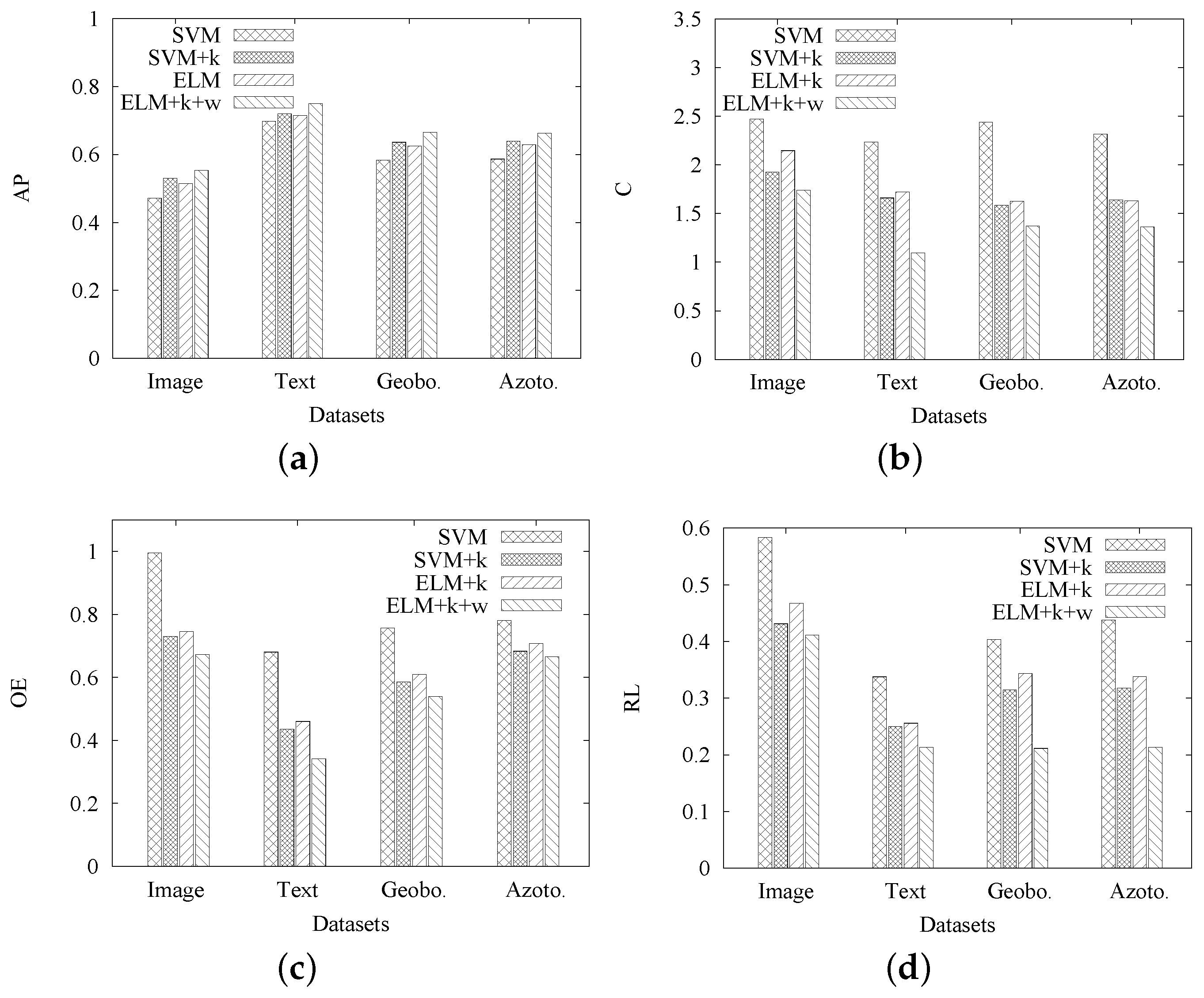
Moreover, we conduct another set of experiments to gradually evaluate the effect of each contribution in MIMLELM. That is, we first modify MIMLSVM+ to include the automatic method for k, then use ELM instead of SVM and then include the genetic algorithm-based weights assignment. The effectiveness of each option is gradually tested on four real datasets using our evaluation criteria. The results are shown in Figure 4a–d, where SVM denotes the original MIMLSVM+ [5], SVM+k denotes the modified MIMLSVM+ including the automatic method for k, ELM+k denotes the usage of ELM instead of SVM in SVM+k and ELM+k+w denotes ELM+k, further including the genetic algorithm-based weights assignment. As seen from Figure 4a–d, the options of including the automatic method for k and the genetic algorithm-based weights assignment can make the four evaluation criteria better, while the usage of ELM instead of SVM in SVM+k slightly reduces the effectiveness. Since ELM can reach a comparable effectiveness as SVM at a much faster learning speed, it is the best option to combine the three contributions in terms of both efficiency and effectiveness.

As mentioned, we are the first to utilize ELM in the MIML problem. In this sense, it is more suitable to consider the proposed MIML-ELM as a framework addressing MIML by ELM. In other words, any better variation of ELM can be integrated into this framework to improve the effectiveness of the original one. For example, some recently-proposed methods, RELM [46], MCVELM [47], KELM [48], DropELM [49] and GEELM [50], can be integrated into this framework to improve the effectiveness of MIMLELM. In this subsection, we conducted a special set of experiments to check how the effectiveness of the proposed method could be further improved by utilizing other ELM learning processes instead of the original one. In particular, we replaced ELM exploited in our method by RELM [46], MCVELM [47], KELM [48], DropELM [49] and GEELM [50], respectively. The results of the effectiveness comparison on four different datasets are shown in

Table 6. The effectiveness comparison of Extreme Learning Machine (ELM)and its variants on the Image dataset.

Image	Evaluation Criterion
	AP↑	C↓	OE↓	RL↓
ELM	0.5529	1.7410	0.6720	0.4109
RELM	0.7141	1.2325	0.4757	0.2909
MCVELM	0.7150	1.2239	0.4724	0.2885
KELM	0.7757	1.1346	0.4379	0.2678
DropELM	0.7814	1.1261	0.4347	0.2568
GEELM	0.7781	1.1312	0.4362	0.2667

,

Table 7. The effectiveness comparison of ELM and its variants on the Text dataset.

Text	Evaluation Criterion
	AP↑	C↓	OE↓	RL↓
ELM	0.7492	1.0928	0.3409	0.2132
RELM	0.7857	1.0420	0.3251	0.2033
MCVELM	0.7959	1.0286	0.3209	0.2007
KELM	0.8019	1.0209	0.3185	0.1992
DropELM	0.8113	1.0091	0.3047	0.1906
GEELM	0.7979	1.0260	0.3198	0.2000

,

Table 8. The effectiveness comparison of ELM and its variants on the Geobacter sulfurreducens dataset.

Geob.	Evaluation Criterion
	AP↑	C↓	OE↓	RL↓
ELM	0.6649	1.3720	0.5390	0.2112
RELM	0.7818	1.1668	0.4584	0.1796
MCVELM	0.7892	1.1559	0.4150	0.1626
KELM	0.8088	1.1279	0.4049	0.1586
DropELM	0.8107	1.1253	0.4020	0.1582
GEELM	0.7933	1.1499	0.4109	0.1617

and

Table 9. The effectiveness comparison of ELM and its variants on the Azotobacter vinelandii dataset.

Azoto.	Evaluation Criterion
	AP↑	C↓	OE↓	RL↓
ELM	0.6622	1.3610	0.6658	0.2129
RELM	0.7928	1.1368	0.5561	0.1778
MCVELM	0.7968	1.1235	0.5533	0.1757
KELM	0.8346	1.0907	0.5283	0.1617
DropELM	0.8524	1.0679	0.5172	0.1583
GEELM	0.7997	1.1194	0.5513	0.1650

, respectively. As expected, the results indicates that the effectiveness of our method can be further improved by utilizing other ELM learning processes instead of the original one.

As mentioned, we are the first to utilize ELM in the MIML problem. In this sense, it is more suitable to consider the proposed MIML-ELM as a framework addressing MIML by ELM. In other words, any better variation of ELM can be integrated into this framework to improve the effectiveness of the original one. For example, some recently-proposed methods, RELM [46], MCVELM [47], KELM [48], DropELM [49] and GEELM [50], can be integrated into this framework to improve the effectiveness of MIML-ELM. In this subsection, we conducted a special set of experiments to check how the effectiveness of the proposed method could be further improved by utilizing other ELM learning processes instead of the original one. In particular, we replaced ELM exploited in our method by RELM [46], MCVELM [47], KELM [48], DropELM [49] and GEELM [50], respectively. The results of the effectiveness comparison on four different datasets are shown in Table 6, Table 7, Table 8 and Table 9, respectively. As expected, the results indicate that the effectiveness of our method can be further improved by utilizing other ELM learning processes instead of the original one.

4.4. Efficiency

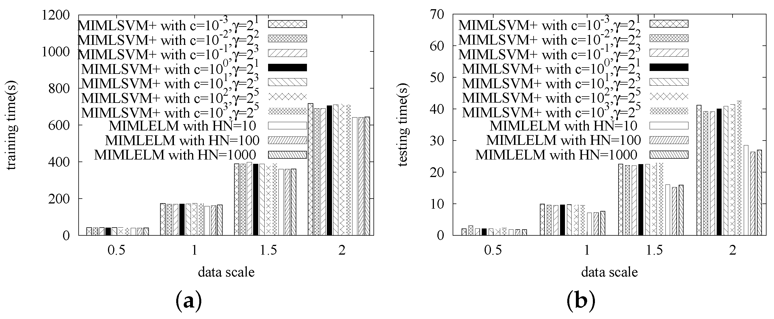
In this series of experiments, we study the efficiency of MIMLELM by testing its scalability. That is, each dataset is replicated different numbers of times, and then, we observe how the training time and the testing time vary with the data size increasing. Again, MIMLSVM+ is utilized as the competitor. Similarly, the MIMLSVM+ algorithm is implemented with a Gaussian kernel, while the penalty factor cost is set from ${10}^{-3}$, ${10}^{-2}$, …, ${10}^3$. The MIMLELM is implemented with the number of hidden layer nodes set to be 100, 200 and 300, respectively.

The experimental results are given in Figure 5, Figure 6, Figure 7 and Figure 8. As we observed, when the data size is small, the efficiency difference between MIMLSVM+ and MIMLELM is not very significant. However, as the data size increases, the superiority of MIMLELM becomes more and more significant. This case is particularly evident in terms of the testing time. In the Image dataset, the dataset is replicated $0.5$–2 times with the step size set to be $0.5$. 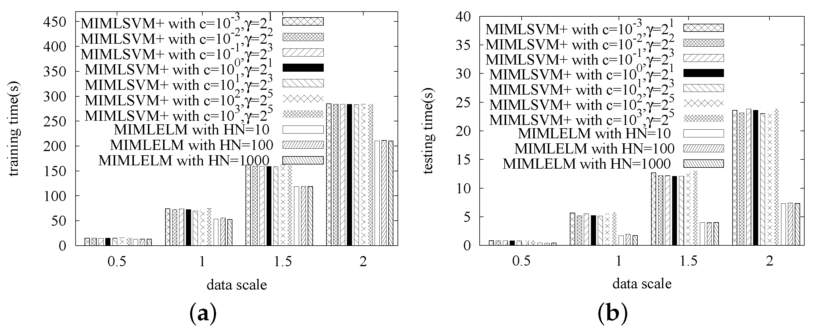When the number of copies is two, the efficiency improvement could be up to one $92.5\%$ (from about $41.2$ s down to about $21.4$ s). In the Text dataset, the dataset is replicated $0.5$–2 times with the step size set to be $0.5$. 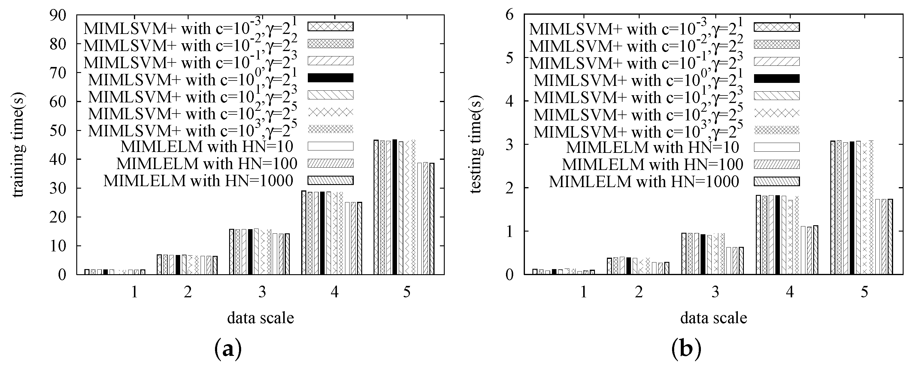When the number of copies is two, the efficiency improvement could be even up to $223.3\%$ (from about $23.6$ s down to about $7.3$ s). In the Geobacter sulfurreducens dataset, the dataset is replicated 1–5 times with the step size set to be 1. 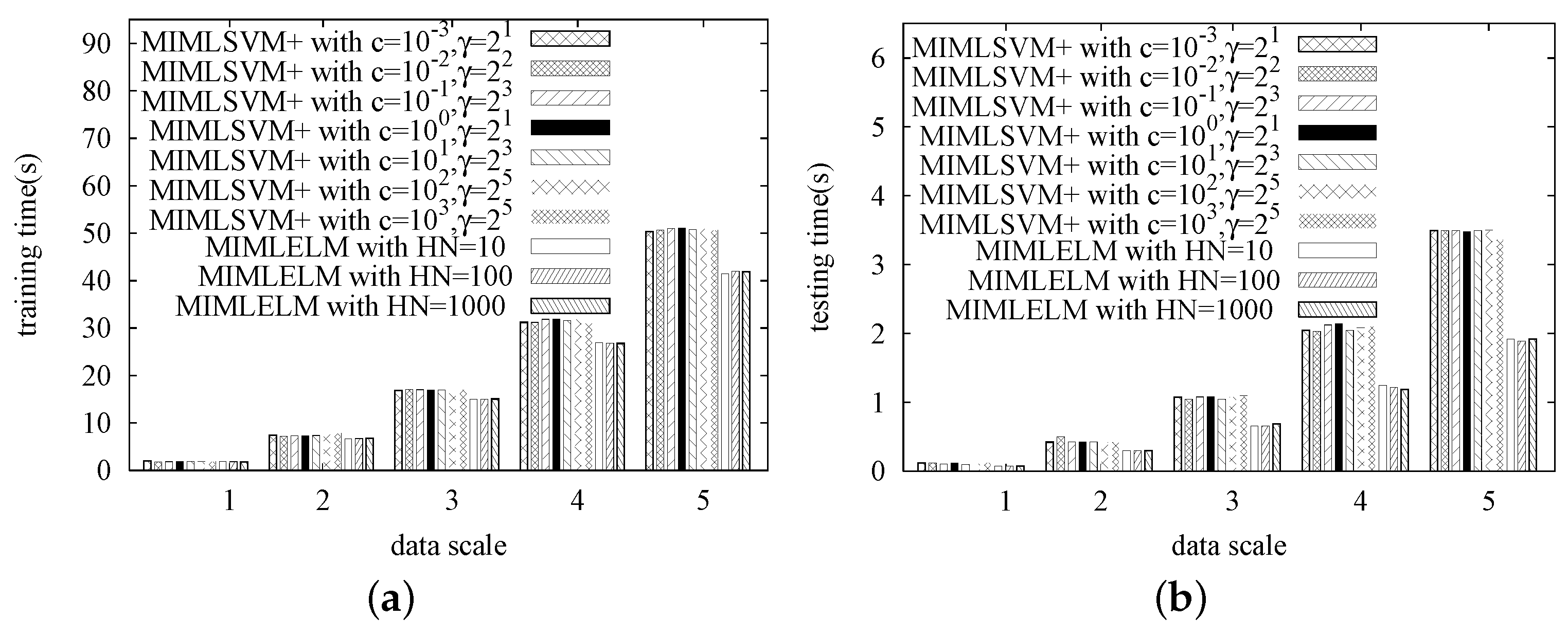When the number of copies is five, the efficiency improvement could be up to $82.4\%$ (from about $3.1$ s down to about $1.7$ s). In the Azotobacter vinelandii dataset, the dataset is replicated 1–5 times with the step size set to be one. When the number of copies is five, the efficiency improvement could be up to $84.2\%$ (from about $3.5$ s down to about $1.9$ s).

4.5. Statistical Significance of the Results

For the purpose of exploring the statistical significance of the results, we performed a nonparametric Friedman test followed by a Holm post hoc test, as advised by Demsar [45] to statistically compare algorithms on multiple datasets. Thus, the Friedman and the Holm test results are reported, as well.

The Friedman test [51] can be used to compare k algorithms over N datasets by ranking each algorithm on each dataset separately. The algorithm obtaining the best performance gets the rank of 1, the second best ranks 2, and so on. In case of ties, average ranks are assigned. Then, the average ranks of all algorithms on all datasets is calculated and compared. If the null hypothesis, which is all algorithms are performing equivalently, is rejected under the Friedman test statistic, post hoc tests, such as the Holm test [52], can be used to determine which algorithms perform statistically different. When all classifiers are compared with a control classifier and $p_1$≤$p_2$≤…≤$p_{k-1}$, Holm’s step-down procedure starts with the most significant p value. If $p_1$ is below $\alpha /(k-1)$, the corresponding hypothesis is rejected, and we are allowed to compare $p_2$ to $\alpha /(k-2)$. If the second hypothesis is rejected, the test proceeds with the third, and so on. As soon as a certain null hypothesis cannot be rejected, all of the remaining hypotheses are retained, as well.

In Figure 4a–d, we have conducted a set of experiments to gradually evaluate the effect of each contribution in MIMLELM. That is, we first modify MIMLSVM+ to include the automatic method for k, then use ELM instead of SVM and then include the genetic algorithm-based weights assignment. The effectiveness of each option is gradually tested on four real datasets using four evaluation criteria. In order to further explore if the improvements are significantly different, we performed a Friedman test followed by a Holm post hoc test. In particular,

Table 10. Friedman test of the gradual effectiveness evaluation on criterion C.

C↓	Image	Text	Geob.	Azoto.	average rank
SVM	2.4712(4)	2.235(4)	2.439(4)	2.317(4)	4
SVM + k	1.9257(2)	1.66(2)	1.5833(2)	1.6391(3)	2.25
ELM + k	2.1451(3)	1.7198(3)	1.6247(3)	1.6285(2)	2.75
ELM + k + w	1.741(1)	1.0928(1)	1.372(1)	1.361(1)	1

shows the rankings of each contribution on each dataset over criterion C. According to the rankings, we computed ${\chi }_F^2=\frac{12\times 4}{4\times 5}\times [(4^2+2.{25}^2+2.{75}^2+1^2)-\frac{4\times 5^2}{4}]=11.1$ and $F_F$ = $\frac{3\times 11.1}{4\times 3-11.1}$ = 37. With four algorithms and four datasets, $F_F$ is distributed according to the F distribution with $4-1=3$ and $(4-1)\times (4-1)=9$ degrees of freedom. The critical value of $F(3,9)$ for α = $0.05$ is $3.86$, so we reject the null-hypothesis. That is, the Friedman test reports a significant difference among the four methods. In what follows, we choose ELM+k+w as the control classifier and proceed with a Holm post hoc test. As shown in

Table 11. Holm test of the gradual effectiveness evaluation on criterion C.

i	Classifier	$\mathit{z}\mathbf{=}\mathbf{(}{\mathit{R}}_{\mathit{i}}\mathbf{-}{\mathit{R}}_{\mathbf{0}}\mathbf{)}\mathbf{/}\mathit{SE}$	p	$\mathit{\alpha }\mathbf{/}\mathbf{(}\mathit{k}\mathbf{-}\mathit{i}\mathbf{)}$
1	SVM	(4 − 1)/0.913 ≈ 3.286	0.0014	$0.017$
2	ELM + k	(2.75 − 1)/0.913 ≈ 1.917	0.0562	0.025
3	SVM + k	(2.25 − 1)/0.913 ≈ 1.369	0.1706	0.05

, with $SE$ = $\sqrt{\frac{4\times 5}{6\times 4}}$ = $0.913$, the Holm procedure rejects the first hypothesis, since the corresponding p value is smaller than the adjusted α. Thus, it is statically believed that our method, i.e., ELM+k+w, has a significant performance improvement of criterion C over SVM. The similar cases can be found when the tests are conducted on the other three criteria. Limited by space, we do not show them here.

In Table 2, Table 3, Table 4 and Table 5, we compared the effectiveness of MIMLSVM+ and MIMLELM with different condition settings on four criteria, where, for a fair performance comparison, MIMLSVM+ is modified to include the automatic method for k and the genetic algorithm-based weights assignment as MIMLELM does.

Table 12. Friedman test of the effectiveness comparison in Table 2, Table 3, Table 4 and Table 5 on criterion C.

C↓		Image	Text	Geob.	Azoto.	average rank
MIMLSVM+	$Cost={10}^{-3},\gamma =2^1$	1.2100(3)	1.0295(4)	1.5122(10)	1.3171(5)	5.5
	$Cost={10}^{-2},\gamma =2^2$	1.1201(1)	1.0405(6)	1.2439(6)	1.0732(3)	4
	$Cost={10}^{-1},\gamma =2^3$	1.1262(2)	1.0445(7)	1.0488(1)	1.1707(4)	3.5
	$Cost=1,\gamma =2^1$	1.9808(7)	1.0145(2)	1.0732(2)	1.0488(5)	3.25
	$Cost={10}^1,\gamma =2^3$	1.9999(8)	1.0041(1)	1.1707(4)	1.0244(5)	5.5
	$Cost={10}^2,\gamma =2^5$	1.9799(6)	1.0450(8)	1.1219(3)	1.9512(9)	6.5
	$Cost={10}^3,\gamma =2^5$	2.0000(9.5)	1.0245(3)	1.2195(5)	1.9756(10)	6.875
MIMLELM	$HN=100$	2.0000(9.5)	1.0670(9)	1.3902(8)	1.4732(8)	8.625
	$HN=200$	1.7410(5)	1.0928(10)	1.3720(7)	1.3610(6)	7
	$HN=300$	1.5700(4)	1.0365(5)	1.4025(9)	1.4585(7)	6.25

shows the rankings of 10 classifiers on each dataset over criterion C. According to the rankings, we computed ${\chi }_F^2$ = $\frac{12\times 4}{10\times 11}$ × $[(5.5^2+4^2+3.5^2+3.{25}^2+3.5^2+6.5^2+6.{875}^2+8.{625}^2+7^2+6.{25}^2)-\frac{10\times {11}^2}{4}]$ ≈ $13.43$ and $F_F$ = $\frac{3\times 13.43}{4\times 9-13.43}$ ≈ $1.79$. With 10 classifiers and four datasets, $F_F$ is distributed according to the F distribution with 10−1 = 9 and $(10$ − $1)$ × $(4$ − $1)$ = 27 degrees of freedom. The critical value of $F(9,27)$ for α = $0.05$ is $2.25$. Thus, as expected, we could not reject the null-hypothesis. That is, the Friedman test reports that there is not a significant difference among the ten methods on criterion C. This is because what we proposed in this paper is a framework. Equipped with the framework, the effectiveness of MIML can be improved further no matter whether SVM or ELM is explored. Since ELM is comparable to SVM on effectiveness [6,32,37], MIMLELM is certainly comparable to MIMLSVM+ on effectiveness. This confirms the general effectiveness of the proposed framework. Similar cases can be found when the tests are conducted on the other three criteria. Limited by space, we do not show them here.

In Figure 5, Figure 6, Figure 7 and Figure 8, we studied the training time and the testing time of MIMLSVM+ and MIMLELM for the efficiency comparison, respectively. In order to further explore if the differences are significant, we performed a Friedman test followed by a Holm post hoc test. In particular,

Table 13. Friedman test of the training time.

Training Time↓		Image	Text	Geob.	Azoto.	average rank
MIMLSVM+	$Cost={10}^{-3},\gamma =2^1$	717.6202(10)	284.75(10)	46.582(8)	50.3727(4)	8
	$Cost={10}^{-2},\gamma =2^2$	690.1484(4)	283.86(7)	46.41(6)	50.6691(6)	5.75
	$Cost={10}^{-1},\gamma =2^3$	690.2365(5)	284.02(8)	46.27(5)	50.9343(8)	6.5
	$Cost=1,\gamma =2^1$	706.2458(6)	283.65(6)	46.8(9)	51.0591(10)	7.75
	$Cost={10}^1,\gamma =2^3$	710.6634(7)	283.21(4)	46.036(4)	50.7315(7)	5.5
	$Cost={10}^2,\gamma =2^5$	717.3216(8)	283.59(5)	46.4272(7)	50.9344(9)	7.25
	$Cost={10}^3,\gamma =2^5$	711.5548(9)	284.47(9)	46.8312(10)	50.5936(5)	8.25
MIMLELM	$HN=100$	641.3661(1)	210.55(2)	38.657(2)	41.4495(1)	1.5
	$HN=200$	642.1002(2)	211.29(3)	38.922(3)	41.9643(3)	2.75
	$HN=300$	644.2047(3)	209.84(1)	38.641(1)	41.9019(2)	1.75

shows the rankings of 10 classifiers on each dataset over training time. According to the rankings, we computed ${\chi }_F^2$ = $\frac{12\times 4}{10\times 11}$ × $[(8^2+5.{75}^2+6.5^2+7.{75}^2+5.5^2+7.{25}^2+8.{25}^2+1.5^2+2.{75}^2+1.{75}^2)-\frac{10\times {11}^2}{4}]$ ≈ $26.45$ and $F_F$ = $\frac{3\times 26.45}{4\times 9-26.45}$ ≈ $8.31$. With ten classifiers and four datasets, $F_F$ is distributed according to the F distribution with $10-1=9$ and $(10-1)\times (4-1)=27$ degrees of freedom. The critical value of $F(9,27)$ for α = $0.05$ is $2.25$, so we reject the null-hypothesis. That is, the Friedman test reports a significant difference among the ten methods. In what follows, we choose ELM with $HN$ = 100 as the control classifier and proceed with a Holm post hoc test. As shown in

Table 14. Holm test of the training time.

i	Classifier	$\mathit{z}\mathbf{=}\mathbf{(}{\mathit{R}}_{\mathit{i}}\mathbf{-}{\mathit{R}}_{\mathbf{0}}\mathbf{)}\mathbf{/}\mathit{SE}$	p	$\mathit{\alpha }\mathbf{/}\mathbf{(}\mathit{k}\mathbf{-}\mathit{i}\mathbf{)}$
1	$cost={10}^3,\gamma =2^5$	(8.25 − 1.5)/2.141 ≈ 3.153	0.00194	0.00556
2	$cost={10}^{-3},\gamma =2^1$	(8 − 1.5)/2.141 ≈ 3.036	0.027	0.00625
3	$cost={10}^0,\gamma =2^1$	(7.75 − 1.5)/2.141 ≈ 2.919	0.0036	0.00714
4	$cost={10}^2,\gamma =2^5$	(7.25 − 1.5)/2.141 ≈ 2.686	0.0074	0.00833
5	$cost={10}^{-1},\gamma =2^3$	(6.5 − 1.5)/2.141 ≈ 2.335	0.0198	0.00396
6	$cost={10}^{-2},\gamma =2^2$	(5.75 − 1.5)/2.141 ≈ 1.985	0.0478	0.001195
7	$cost={10}^1,\gamma =2^3$	(5.5 − 1.5)/2.141 ≈ 1.868	0.0628	0.0167
8	HN = 200	(2.75 − 1.5)/2.141 ≈ 0.584	0.562	0.025
9	HN = 300	(1.75 − 1.5)/2.141 ≈ 0.117	0.912	0.005

, with $SE$ = $\sqrt{\frac{10\times 11}{6\times 4}}$ = $2.141$, the Holm procedure rejects the hypotheses from the first to the fourth since the corresponding p-values are smaller than the adjusted α’s. Thus, it is statically believed that MIMLELM with $HN$ = 100 has a significant performance improvement of training over most of the MIMLSVM+ classifiers. Similarly,

Table 15. Friedman test of the testing time.

Testing Time↓		Image	Text	Geob.	Azoto.	average rank
MIMLSVM+	$Cost={10}^{-3},\gamma =2^1$	41.1999(8)	23.587(7)	3.0732(7.5)	3.4944(7.5)	7.5
	$Cost={10}^{-2},\gamma =2^2$	39.2343(5)	23.148(5)	3.0888(10)	3.4944(7.5)	6.875
	$Cost={10}^{-1},\gamma =2^3$	39.1066(4)	23.834(9)	3.042(4)	3.4944(7.5)	6.125
	$Cost=1,\gamma =2^1$	40.0244(6)	23.615(8)	3.0576(6)	3.4788(5)	6.25
	$Cost={10}^1,\gamma =2^3$	40.8324(7)	23.012(4)	3.0732(7.5)	3.4944(7.5)	6.5
	$Cost={10}^2,\gamma =2^5$	41.3534(9)	23.465(6)	3.053(5)	3.4976(10)	7.5
	$Cost={10}^3,\gamma =2^5$	742.439(10)	23.936(10)	3.0786(9)	3.3634(4)	8.25
MIMLELM	$HN=100$	28.5014(3)	7.3164(1)	1.7316(2)	1.9188(2.5)	2.125
	$HN=200$	26.4258(1)	7.4256(3)	1.7316(2)	1.8876(1)	1.75
	$HN=300$	27.0154(2)	7.3457(2)	1.7316(2)	1.9188(2.5)	2.125

shows the rankings of 10 classifiers on each dataset over testing time. According to the rankings, we computed ${\chi }_F^2$ = $\frac{12\times 4}{10\times 11}$ × $[(7.5^2+6.{875}^2+6.{125}^2+6.{25}^2+6.5^2+7.5^2+8.{25}^2+2.{125}^2+1.{75}^2+2.{125}^2)-\frac{10\times {11}^2}{4}]$ ≈ $24.55$ and $F_F$ = $\frac{3\times 24.55}{4\times 9-24.55}$ ≈ $6.43$. With ten classifiers and four datasets, $F_F$ is distributed according to the F distribution with $10-1=9$ and $(10-1)\times (4-1)=27$ degrees of freedom. The critical value of $F(9,27)$ for α = $0.05$ is $2.25$, so we reject the null-hypothesis. That is, the Friedman test reports a significant difference among the ten methods. In what follows, we choose ELM with $HN$ = 200 as the control classifier and proceed with a Holm post hoc test. As shown in

Table 16. Holm test of the testing time.

i	Classifier	$\mathit{z}\mathbf{=}\mathbf{(}{\mathit{R}}_{\mathit{i}}\mathbf{-}{\mathit{R}}_{\mathbf{0}}\mathbf{)}\mathbf{/}\mathit{SE}$	p	$\mathit{\alpha }\mathbf{/}\mathbf{(}\mathit{k}\mathbf{-}\mathit{i}\mathbf{)}$
1	$cost={10}^3,\gamma =2^5$	(8.25 − 1.75)/2.141 ≈ 3.036	0.0027	0.00556
2	$cost={10}^{-3},\gamma =2^1$	(7.5 − 1.75)/2.141 ≈ 2.686	0.047	0.00625
3	$cost={10}^2,\gamma =2^5$	(7.5 − 1.75)/2.141 ≈ 2.686	0.047	0.00714
4	$cost={10}^{-2},\gamma =2^2$	(6.875 − 1.75)/2.141 ≈ 2.394	0.0168	0.00833
5	$cost={10}^1,\gamma =2^3$	(6.5 − 1.75)/2.141 ≈ 2.219	0.0272	0.00396
6	$cost=1,\gamma =2^{1}5$	(6.25 − 1.75)/2.141 ≈ 2.102	0.0358	0.001195
7	$cost={10}^{-1},\gamma =2^3$	(6.125 − 1.75)/2.141 ≈ 2.043	0.0414	0.00167
8	HN = 100	(2.125 − 1.75)/2.141 ≈ 0.175	0.865	0.025
9	HN = 300	(2.125 − 1.75)/2.141 ≈ 0.175	0.865	0.005

, with $SE$ = $\sqrt{\frac{10\times 11}{6\times 4}}$ = $2.141$, the Holm procedure rejects the hypotheses from the first to the third since the corresponding p-values are smaller than the adjusted α’s. Thus, it is statically believed that MIMLELM with $HN$ = 200 has a significant performance improvement of training over two of the MIMLSVM+ classifiers.

In summary, the proposed framework can significantly improve the effectiveness of MIML learning. Equipped with the framework, the effectiveness of MIMLELM is comparable to that of MIMLSVM+, while the efficiency of MIMLELM is significantly better than that of MIMLSVM+.

5. Conclusions

MIML is a framework for learning with complicated objects and has been proven to be effective in many applications. However, the existing two-phase MIML approaches may suffer from the effectiveness problem arising from the user-specific cluster number and the efficiency problem arising from the high computational cost. In this paper, we propose the MIMLELM approach to learn with MIML examples quickly. On the one hand, the efficiency is highly improved by integrating extreme learning machine into the MIML learning framework. To our best knowledge, we are the first to utilize ELM in the MIML problem and to conduct the comparison of ELM and SVM on MIML. On the other hand, we develop a method of theoretical guarantee to determine the number of clusters automatically and to exploit a genetic algorithm-based ELM ensemble to further improve the effectiveness.