Article

Performance Study of a Fluidic Hammer Controlled by an Output-Fed Bistable Fluidic Oscillator

1
Key Laboratory of Ministry of Land and Resources on Complicated Conditions Drilling Technology, Jilin University, Changchun 130026, China
2
College of Construction Engineering, Jilin University, Changchun 130026, China
*
Authors to whom correspondence should be addressed.
Appl. Sci. 2016, 6(10), 305; https://doi.org/10.3390/app6100305
Submission received: 7 September 2016 / Revised: 13 October 2016 / Accepted: 13 October 2016 / Published: 20 October 2016

Abstract

:
Using a no-moving-component output-fed bistable fluidic oscillator to control fluid flows into a parallel path has been recognized for a considerable time, but as yet it is not so widely adopted as its obvious benefits would deserve. This may be attributed to the encountered problems associated with its jet behavior, complicated by its loading characteristics. In order to investigate a typical case for the application of the output-fed fluidic oscillator, this paper elaborates on the computational fluid dynamics (CFD) simulation method for studying the performance of a fluidic hammer controlled by an output-fed bistable fluidic oscillator. Given that couple mechanism exists between the flow field in the fluidic oscillator and the impact body, dynamic mesh technique and a user-defined function written in C programming language were used to update the mesh in the simulations. In terms of the evaluation of performance, the focus is on the single-impact energy and output power of the fluidic hammer in this study, to investigate the effect of different parameters of the impact body on them. Experimental tests based on the noncontact measuring method were conducted to verify the simulation results, by which the accuracy and reliability of this CFD simulation method was proved.

Graphical Abstract

1. Introduction

Fluidic oscillators, based on the well-known Coanda effect [1] of jet attachment to a wall, are considered to be able to generate a self-sustained periodic oscillating jet without the necessity of any movable or deformable parts [2,3]. Like other fluidic devices, they are compact, reliable, and robust, while exhibiting resistance to high temperatures, corrosive environments, and other extreme ambient conditions, which offers attractive application possibilities in furnaces, nuclear radiation, and other unusual conditions [4].
Various designs of fluidic oscillators have been proposed and investigated by previous researchers [5,6,7,8]. The most common fluidic oscillators are those with a jet-deflection amplifier and destabilizing feedback loops based on the fundamental operating principles associated with the two classic designs [7,9]: relaxation oscillator with a single loop (shown in Figure 1a) and the two-loops version, namely, negative feedback oscillator (shown in Figure 1b). Behavior of both is characterized by oscillating frequency increasing linearly in proportion to the inlet flow rate, leading to the wide application of them to the measurement of flow rates [10]. Besides, because of the oscillating features, they are also widely applied for mixers [11], sensors [12], and memory and control devices [13]. Another less common fluidic oscillator, as displayed in Figure 1c, is the resonance-channel fluidic oscillator, recently proposed by Tesař [14]. Instead of the flow signal propagating in loops, the flow in the resonance-channel fluidic oscillator is here switched by the action of pressure waves traveling in a resonance channel connected to one of the control nozzles. The oscillation frequency of the resonance-channel fluidic oscillator is determined by the length of the resonance channel and the propagation velocity, but does not depend on the flow rate passing through the oscillator [15]. This novel fluidic oscillator is widely used for flow-separation control [16].
In a fluidic oscillator, the available pressure energy of the fluid feed is converted, in the supply nozzle, into the kinetic energy of jet, creating a very low-pressure region in the space between the two attachment walls, and then, the kinetic energy is reconverted back into the pressure energy form at the entrance of the output channel. Due to this energy reconversion mechanism, the fluidic oscillators have been recognized as particularly desirable to serve as actuators, assisting in output force, moment, or torque, as the supplied flow alternatively flows into the output channels. One of the successful designs is the output-fed bistable fluidic oscillator is shown in Figure 1d. A striking feature of the output-fed bistable fluidic oscillator is the introduction of vents and the non-coplanar setting of feedback loops, making the fluidic oscillator become jet-switching insensitive. The supply jet would not detach from the wall and switch to the other attachment wall unless the hydraulic resistance downstream of the output channel met at a certain level. This working principle focuses more on fluid flow control, which is similar to the function of a fluidic amplifier. Given this, the performance of the output-fed bistable fluidic oscillator can be evaluated both as a fluidic oscillator and a fluidic amplifier. This distinctive feature makes the output-fed bistable fluidic oscillator very unique compared with the two classic types mentioned above, and makes a wide application for engineering practice since it was first suggested and patented in the 1970s. For instance, with the combination of an output-fed bistable fluidic oscillator and the friction reduction technology, He et al. [17] proposed a novel drilling tool to reduce the drag and torque in horizontal directional drilling process. Xue et al. [18] investigated a booster compressor worked in an ultrahigh-pressure-jet system, in which an output-fed bistable fluidic oscillator represents the core part for compressor-reversing control. Additionally, in the refrigeration system, Luo et al. [19,20] utilized an output-fed bistable fluidic oscillator in a submersible pump to control cryogenic coolant cycling in a pressure-coring system. Much more commonly, the output-fed bistable fluidic oscillator was used as an actuator in a fluidic hammer [21,22] which is a down-the-hole (DTH) hammer drilling tool widely used in deep hole drilling, geothermal drilling, and drilling in the oil and gas industry.
Most previous work on a fluidic oscillator or a fluidic amplifier has usually been based on computational fluid dynamics (CFD) simulation and experimental study in a steady or quasi-steady state [7,23,24,25], as their loading characteristics are constant or varying in a certain level. However, for the output-fed bistable fluidic oscillator, the loading characteristics are very special and influential to its oscillating behavior. The nonlinear loading variation results in a complex coupling relationship between the fluid flow in the fluidic oscillator and the load downstream from the output channel. Hence performance analysis on an isolated output-fed bistable fluidic oscillator is not sufficient and is somewhat unreasonable. Therefore, for reaching satisfactory results, transient study coupled with the variation of load is necessary.
In order to focus on the basic issues, this paper concentrates on the relatively typical case of an output-fed bistable fluidic oscillator controlling an impact body to implement reciprocating movement (i.e., the fluidic hammer). The objective of this study is to investigate the effects posed by some of the important geometric and operational parameters and loading characteristics on the performance of the fluidic hammer using the CFD transient analysis method and the experimental validation, thus reaching an improvement of performance for the fluidic hammer and providing a research method for further analogous investigations related to the output-fed bistable fluidic oscillator.

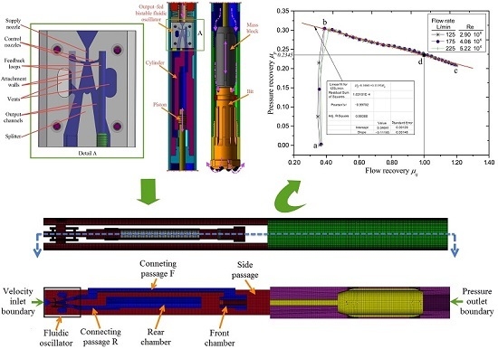
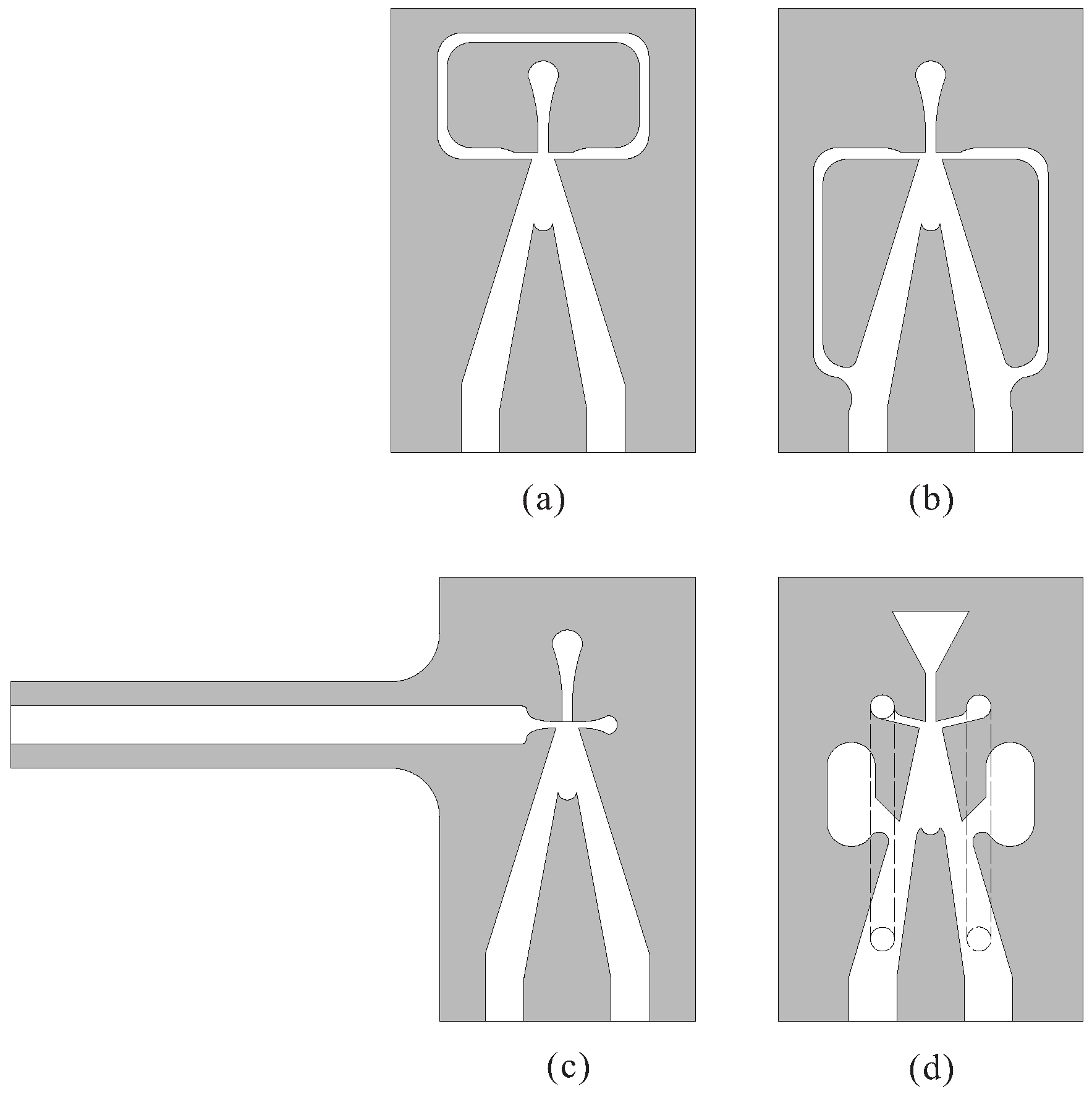
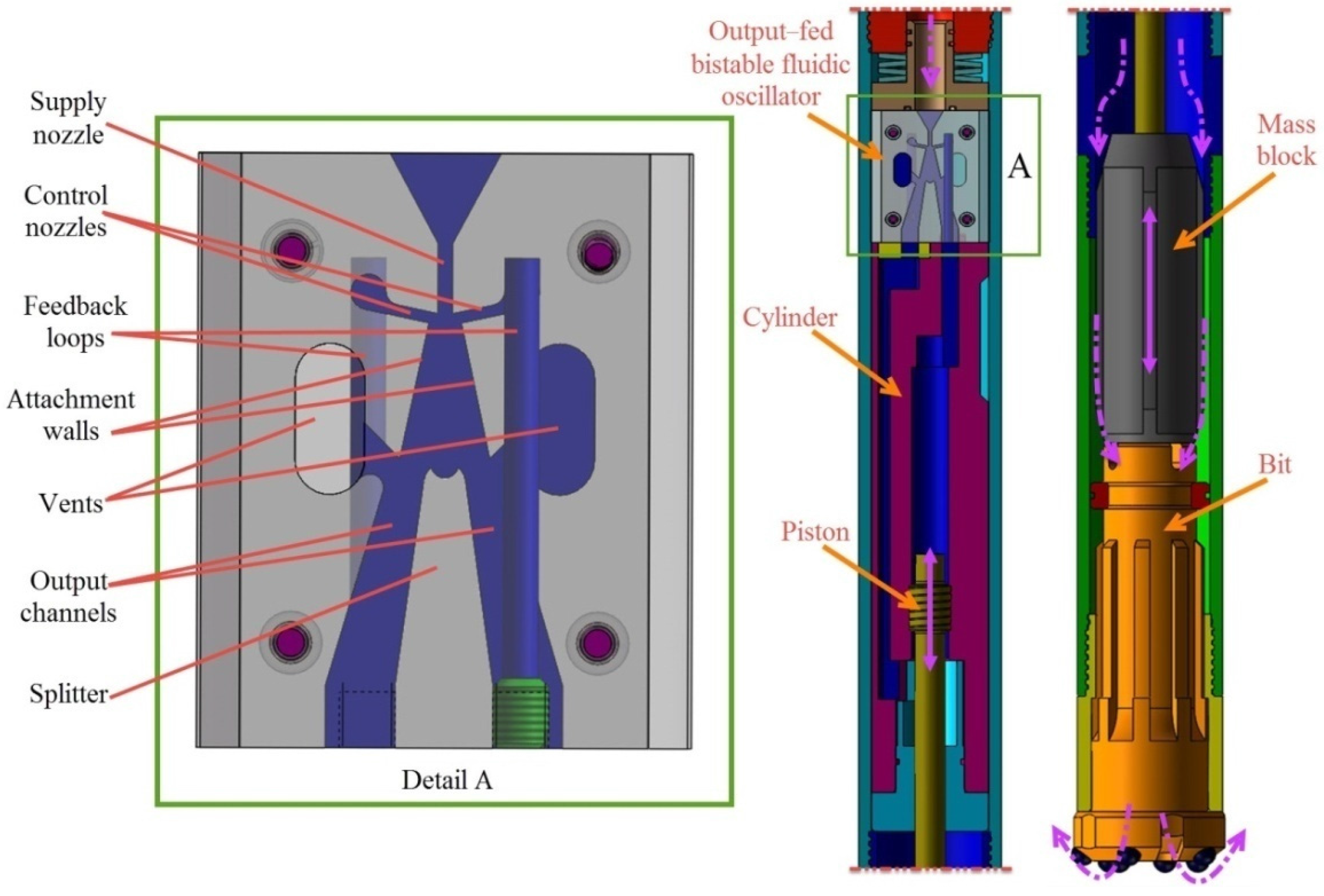
2. Description of the Fluidic Hammer

As shown in Figure 2, a fluidic hammer consists of several major components, namely, an output-fed bistable fluidic oscillator, a cylinder, a piston, a mass block, and a bit. The piston divides the cylinder into two working chambers: the front chamber and the rear chamber. The piston and the mass block are connected to each other by the tapered interference fit to form an impact body. The output-fed bistable fluidic oscillator is employed to regulate the impact body to move forth and back.
When the fluidic hammer works normally, the high pressure liquid enters the fluidic oscillator through the supply nozzle and is turned into a jet with relatively large kinetic energy in the interaction region. Because of the transversal pressure difference produced by the unbalance of entrainment of the surrounding liquid, the jet will deflect to one side of the adjacent attachment wall and enter one of the chambers of the cylinder through the output channel, thus pushing the impact body to move forth or back. When the impact body reaches one of its stroke ends, a large pressure pulsation charged with high-pressure energy will be produced in the output channel caused by sudden stop of the impact body. Part of the pressure pulsation propagates along the feedback loop to the outlet of the control nozzle on the deflected jet side, where the pressure energy is converted into kinetic energy of liquid, exerting a transverse force and flow momentum on the supply jet, thus triggering the supply jet to detach from the initially attached side wall and attach onto the other side. This detachment and attachment process continues, leading to the periodic oscillation and the reciprocating movement of the impact body, thereby generating persistent periodic impact force acting on the drill bit.

3. Numerical Procedure

3.1. SpecifiedDimensions of Output-Fed Bistable Fluidic Oscillator

The representative geometry parameters of the output-fed bistable fluidic oscillator investigated in this work is shown in Figure 3. All cavities forming the fluidic oscillator are of the same depth. Design of the fluidic oscillator, based on the relatively delicate interaction of fluid mechanical phenomena, is no simple task. It takes a considerable effort to get the fluidic oscillator to work successfully in the fluidic hammer on the laboratory bench. The fluidic oscillator used in this study is designed on the basis of a recent favorable experience and successfully applied in field tests. In designing of the fluidic oscillator, the width of the supply nozzle was served as the reference parameter used to determine the other geometric parameters. The specified dimensions of the output-fed bistable fluidic oscillator is shown in Table 1.

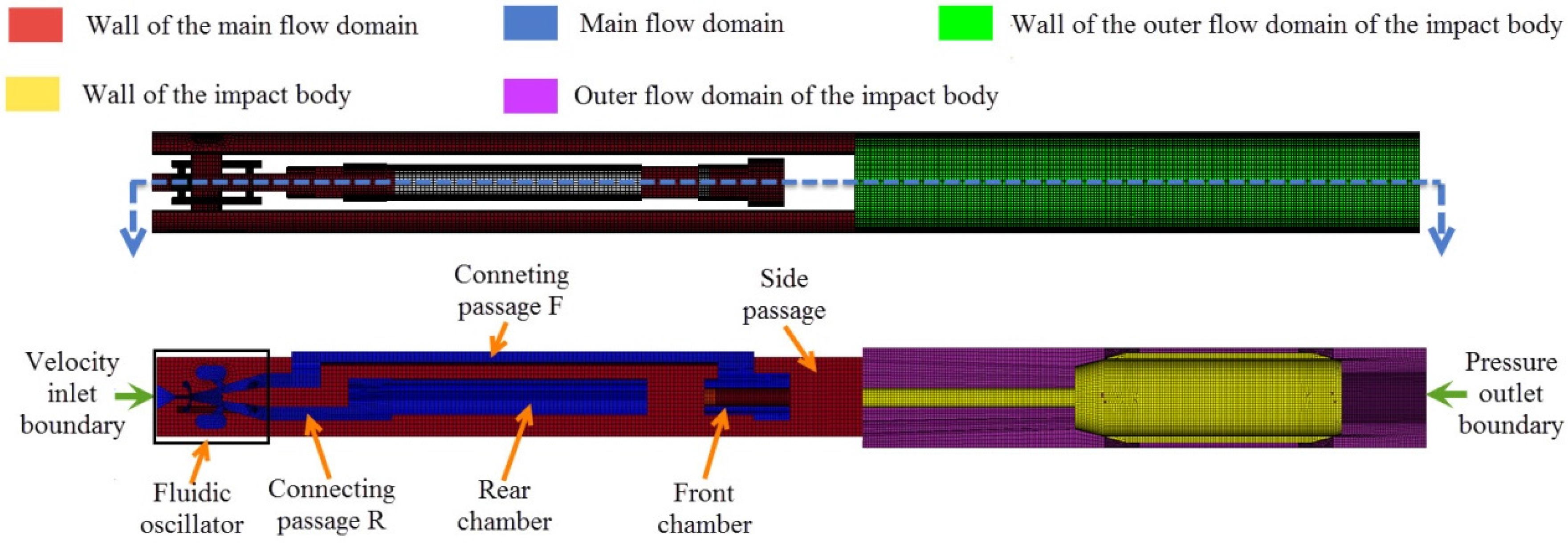
3.2. Methodology of Simulation and Computational Domains

The flow fields of fluidic oscillators are similar to that of the fluidic devices which have been numerically andexperimentally investigated.Tesař and Bandalusena [26] performed a study, by means of CFD computations and PIV (Particle Image Velocimetry) measurements, aimed at clarifying the behavior of a typical fluidic valve at low Reynolds numbers. By using simplified 2D computation CFD models, Wang et al. [27] investigated the effect of varying structural parameters on the flow characteristics of the fluidic flowmeter, and they found that the numerical results were consistent with the experimental results. In order to investigate the flow behavior in monostable mini- and micro-oscillators, Rachid et al. [28] proposed a hybrid simulation approach, which consists both of the 2D CFD simulation and analytical modeling method. Presumably due to the traditional planar design of the fluidic devices, the challenges existing in the difficulty of convergence, and huge demand on computer resources, there have been fewer CFD studies based on the 3D computational models on fluidic oscillators than other numerical studies, namely, the use of 2D simulation models or the analytical modeling. Considering that the relaxation bistable oscillator is a 2D analogue of the Tesar–Zimmerman oscillator [29] (3D feedback loops), the output-fed bistable fluidic oscillator studied here can certainly loop around the vents in 2D topologically. However, for an output-fed bistable fluidic oscillator in the fluidic hammer, the movement of the impact body is influential to the oscillating behavior of the oscillator. There exists acomplex coupling relationship between the fluid flow in the output-fed fluidic oscillator and the movement of the impact body. Simulations on an isolated output-fed bistable fluidic oscillator are deficient and unreasonable. In the fluidic hammer, because of the nonplanar cylinder and the impact body, the fluid flows in the working chambers and the passages connecting them are not planar or axisymmetric, thus the use of 2D computational models are apparently not suitable. Besides, in order to retain a high level of predictive accuracy, analytical modeling method depending heavily on experimental data is not desirable.
The above review points out the need to use more elaborated models to simulate the fluid flow inside an output-fed bistable fluidic oscillator coupling with the movement of the impact body. The dynamic mesh modeling technique using 3D computational models has provided a promising approach to clarify the flow behavior in the fluidic hammer, as the computational domains can be updated automatically at each time step based on the moving positions of the impact body. Therefore, CFD simulation method with the technique of dynamic mesh was used in this study.
The computational flow domain of a typical fluidic hammer includes the flow field of a fluidic oscillator, the front and rear chambers of the cylinder, the connecting passages between the fluidic oscillator and the cylinder, the outer flow field of the impact body, and the side passages connecting with the vents and the outer flow field of the impact body. Three different mesh densities with mesh sizes varying from 180,000 to 750,000 for the fluidic hammer were calculated. After performing the grid independence analysis from the geometry spatial discretization and considering the reasonable computational time and the satisfactory model accuracy, medium grids were used in this study. One of the computational domains is showed in Figure 4. In this grid there are total 368,522 cells, of which 9752 cells are pentahedrons, and the others are hexahedrons.

3.3. Mathematical Formulationfor Dynamic Mesh Modeling

The dynamic mesh modeling method was used to simulate the fluid flow in the fluidic hammer. In CFD simulation, with respect to dynamic meshes, the position of the moving boundaries and objects were changed by the used of FLUENT (Release 6.3.26, Ansys Inc., Pittsburgh, PA, USA) solver and the corresponding grid was adjusted automatically. In an arbitrary control volume V of the computational domain, the calculation follows the mass conservation equation and its integral form can be written as [30]:
d d t V ρ ϕ d V + V ρ ϕ ( u u g ) d A = V Γ ϕ · d A + V S ϕ d V
where ρ is the fluid density, u is the flow velocity vector, u g is the grid velocity of the moving mesh, A is the area vector, Γ is the diffusion coefficient, and S ϕ is the source term of flux ϕ .
A first-order backward difference scheme of Equation (1) is presented as follows:
d d t V ρ ϕ d V = ( ρ ϕ V ) n + 1 ( ρ ϕ V ) n Δ t
where n and n+1 denote the quantity at present and next time step of numerical value, respectively. The (n+1)th time step volume Vn+1 can be calculated from Equation (3):
V n + 1 = V n + d V d t Δ t

3.4. Boundary Conditions and Solving Strategies

There are two stages for the simulation of a fluidic hammer—the steady computation and the transient computation. The transient computation is based on the results of the steady computation. In the simulation with steady computation, a 3D double-precision steady-state segregated solver was used in this stage, by which the governing Navier–Stokes equations were solved until defined values of convergence were met [31]. As displayed in Figure 4, a velocity inlet boundary condition was adopted at the inlet of the fluidic oscillator, and a pressure outlet boundary was applied at the bottom face of the outer flow domain of the impact body. The pressure outlet boundary condition was set to atmospheric pressure. Besides, the no-slip boundary conditions were adopted for all the walls. In the other stage of transient simulation, boundary conditions were kept exactly the same as in the steady simulation. While the segregated solver was switched to unsteady-state, user-defined functions (UDFs) written in C programming language were employed to describe the motion of any moving rigid surface in the computational domain. According to the time-step length independence study, the time step in the transient simulation was set to 1E-4s, which is reasonable and short enough to capture details of the wall attachment switching process of the main jet. Moreover, the time cost of calculation is acceptable with the setting time step.
The internal fluid flow of a fluidic hammer is assumed to be incompressible and the body force of internal fluid is ignored; besides, no heat exchange occurs between the liquid and its surroundings. In order to deal with the coupling of velocity and pressure, the well-known SIMPLE (Semi-Implicit Method for Pressure-Linked Equations) strategy was used due to the reasonable accuracy and relative low calculation cost [32]. The PRESTO (pressure staggered option), a pressure interpolation scheme that is beneficial for predicting the highly swirling flow characteristics prevailing inside the fluidic amplifier, was adopted [33]. As the dynamic mesh method only works with the first-order time advancement at present, the first-order upwind scheme was employed for the discretization [34]. As for the turbulence models in the simulation, the successful applications of the RNG-based κ - ε turbulence model for predicting the complex flow in the fluidic devices has been reported [26]. Thus, the RNG-based κ - ε turbulence model was used in this study.

4. Results and Discussion

4.1. Performance Analysis Related to the Flow Behavior

In order for the wall attachment phenomenon to occur in the interaction region of the output-fed fluidic oscillator, the power stream is accelerated in the converging supply nozzle, and hence its energy is mainly kinetic. In order to drive the impact body to move, it is generally required to convert this dynamic energy into a static pressure that is recoverable at the output channels. This pressure, expressed as a ratio of the power supply pressure, is termed pressure recovery [4,35]. As shown in Figure 5, the static pressure at the vents is used as the reference for evaluation of pressure difference. It is obvious that the pressure there at the vents is essentially equal to atmospheric pressure. The pressure recovery can thus be described as follows:
μ p = P o / P s
Correspondingly, in a similar manner, the flow rate at the output channel can also be nondimensionalized by associating it with the flow rate at the inlet of the supply nozzle. When the liquid flows through the supply nozzle, where it forms a jet, some part of the jet flow enters the output channel. The cylinder receives the output flow captured by the output channel. Because of the motion of the impact body, the output flow is variable. In fact, as shown in Figure 5, the flow rate at the output channel is equal to the moving velocity of the impact body times the liquid action area of the piston. Since the supply flow (volume flow rate) is constant, the ratio between the output flow and the supply flow is determined by the former. This value of the ratio is defined as the flow recovery [4] and can be described by the equation below.
μ q = Q o / Q s = A p v A s u
Since the backward impact regime is useless for rock breaking, in this study we focus more on the forward movement of the impact body. As described in Equation (5), when the supply flow rate Qs is constant, μ q is proportional to v. Higher value of v means lower fluid resistance downstream from the output channel, as a larger portion of liquid flows into the working chamber through the output channel. Therefore, flow recovery represents the loading characteristics of the fluidic hammer to some extent.
As shown in Figure 5, some important parameters of the impact body are displayed; they are Dp, Dr, m, and L. All of these four parameters affect the critical flow velocity of the fluidic oscillator [21], potentially posing significant impacts on the performance of the fluidic hammer. In this study, SC-86H experimental prototype is served as the baseline fluidic hammer for comparison, and the dimensions of the impact body are given in Case 1 of Table 2. In the subsequent sections, the dimensions of the impact body are set to change in the neighborhood of the set value of the baseline fluidic hammer to figure out their effects. Additionally, as the dimension of one parameters varies, the other parameters retain the same values as the baseline fluidic hammer. The dimensions of the parameters in all cases examined in this study are listed in Table 2.
In order to investigate the effect of operational parameter (i.e., supply flow rate) on the flow behavior in the fluidic oscillator, a series of computations were performed on the baseline fluidic hammer. Figure 6 shows the relationship between pressure recovery and flow recovery at different supply flow rate obtained by the CFD simulation. The corresponding Reynolds numbers ranged from 2.90 × 10⁶ to 5.22 × 10⁶. The diagram indicates that μ q is found as a function of μ p and the relationship between them is independent of Reynolds number (or the supply flow rate). The variations of pressure recovery versus flow recovery can be divided into two sections, corresponding to two states of the supply jet. As displayed in Figure 6, at the state of a–b, the pressure recovery changes sharply as the flow recovery increases. It can be thus attributed because of the delay caused by the fluid inertia and the finite time for the acoustic waves propagating in the feedback loops, the jet-switching deflection process has not finished before the impact body rebounds and moves forward. While at the state of b–c, the supply jet has already deflected and switched its attachment to the other side, and drives the impact body to move forward. As shown in Figure 6, the data shown at the section of b–c has a linear fit, made for supply flow rate Qs = 125 L/min. The value of the adjusted squared multiple correlation coefficient is 0.99388, near to 1.0, suggesting that the pressure recovery is simply negatively and linearly related with the flow recovery, and as the value of the flow recovery increases the value of the pressure recovery decreases. The point “d” at the fitting line, where the value of the flow recovery is 1.00, indicates that the flow rate of output flow is equal to that of the supply flow. As the flow recovery increases continuously, there will be extra liquid entrained into the output channel due to the escalating jet-pump effect caused by the diminishing fluid resistance for entering the rear chamber of the cylinder.
In order to make the presentation of the CFD computation results more general and try to find some trace for designing fluidic hammers with high performance, the general form of the fitting line equation is expressed as follows:
μ p = μ p 0 C p q μ q
where the intercept μ p 0 of Equation (6) can be regarded as the value of the pressure recovery when the velocity of the impact body is 0 and thus all of the supply flow is discharged into the vents, and the slope C p q represents a dimensionless characteristic coefficient between the pressure recovery and flow recovery.
Pressure drop Ps can be expressed as:
Ps=u2/2
Combining Equations (4)–(7), the following expression is obtained:
v = ( μ p 0 μ p ) A s u C p q A p = ( ρ μ p 0 u 2 2 P o ) A s u C p q A p ρ u 2
v max = ( μ p 0 μ p min ) A s u C p q A p
where vmax is the maximum value of v, and μ p min is the minimum value of μ p . As shown in Figure 6, when the supply flow rate varies, μ p min remains approximately constant at the vicinity of point c.
The single-impact energy E, is calculated from:
E = m v max 2 / 2
The single-impact energy E is of crucial importance for evaluating the performance of the fluidic hammer, as when the single-impact energy is lower than a certain value, the fluidic hammer can hardly break the corresponding rocks [36,37]. Development of fluidic hammers with great single-impact energy is the current prevailing trend [38,39]. It can be concluded from Equations (9) and (10), when the parameters of the fluidic hammer keep the same, the single-impact energy E is proportional to the square of u or Qs, and without regard to the interaction, smaller areas of As and Ap mean higher single-impact energy.

4.2. The Effect of Parameters of the Impact Body on the Performance of Fluidic Hammers

Apart from the single-impact energy mentioned above, another important performance parameter of the fluidic hammer is the output power which can be written as:
P = E f
In this equation, the output power is proportional to both of the single-impact energy E and the impact frequency f. Case 1–17 form four groups of CFD simulation tests to examine the effect of different parameters of the impact body on the performance of the fluidic hammer. In these simulations, the supply flow rate of the fluidic hammer remains the same at 200 L/min. As shown in Figure 7, the results are obtained from the computations of Case 1–5. It indicates that as the diameter of the piston becomes larger, both of the single-impact energy and the output power exhibit downward trends. On the other hand, the variation of impact frequency of the impact body is not monotone, changing with the diameter of the piston, and reaches its maximum at Dp = 26 mm. This is attributed to the fact that when the diameter of the piston increases, the liquid action areas of the piston increases, which means lower fluid resistance for the output flow entering the working chamber, thus leading to a higher flow recovery and a correspondingly lower pressure recovery. As shown in Equation (12), when the recovered pressure Po decreases and the action area Ap increases, the moving velocity of the impact body can both increase or decrease, which is determined by the ratio of change of Po and Ap. Additionally, when the stroke is constant, the stroke time is reversely proportional to the moving velocity of the impact body. In fact, in this group of examined cases, with the increasing of Dp, the forward stroke time increases while the backward stroke time decreases, and when the variation magnitude of latter is larger, the impact frequency of the impact body will increase (e.g., Dp = 26 mm). In this group of simulations, it can be concluded that a smaller diameter of the piston means better performance of the fluidic hammer, as both its single-impact energy and output power is at its highest.
d v = ( P o A p / m ) d t
Cases 1, 6, 7, 8, and 9 form another group of computations. It can be seen in Figure 8 that there is no corresponding value of E, f, and P for Case 9. This is because the flow velocity in the supply nozzle does not reach the threshold flow velocity [21,22] of the fluidic hammer, thus leading to the result that the supply jet was unable to switch to the other side of the attachment wall. An increase in the diameter of the piston rod means the decrease in the action area of the front chamber of the cylinder, due to the previous conclusion obtained in the earlier group, the impact frequency of the impact body decreases. This is confirmed by the variations of impact frequency shown in Figure 8. The single-impact energy of the impact body firstly increases and then decreases. This increase is mainly due to the decrease of the action force in the front chamber while the decrease can be attributed to the lower rebound velocity and the more delayed switching attachment caused by the decrease of the backward impact velocity when the backward-moving impact body rebounds and starts to move forward. Compared with the impact frequency, the variation amplitude of single-impact energy is relatively weak, and hence as depicted in Figure 8, the output power of the fluidic hammer is in a steady decrease which is consistent with the changing trend of the impact frequency. In this group of simulations, it can be concluded that the cases of Dr = 16 mm or 18mm show better performance, as both of their single-impact energy and output power is relatively high.
Figure 9 shows the computation results of the group including Cases 1, 10, 11, 12, and 13. As the mass of the impact body increases, the single-impact energy of the impact body increases while the impact frequency decreases. The output power of the fluidic hammer does not vary monotonically, and there exists a maximum value at m = 8 kg. In this group of computation cases, the cases of m = 8 kg or 10 kg shows better performance of the fluidic hammer, as both of their single-impact energy and output power is relatively high.
The rest of the cases form the last group of test cases. As shown in Figure 10, an increase of the stroke increases the single-impact energy and decreases the impact frequency, while the output power first increases and then decreases. This phenomenon indicates that the increase in the single-impact energy is more pronounced than the decrease in the impact frequency at the beginning, and then the decrease in the impact frequency is more significant. In this group of simulations, the case of L = 140 mm shows the highest performance of the fluidic hammer.

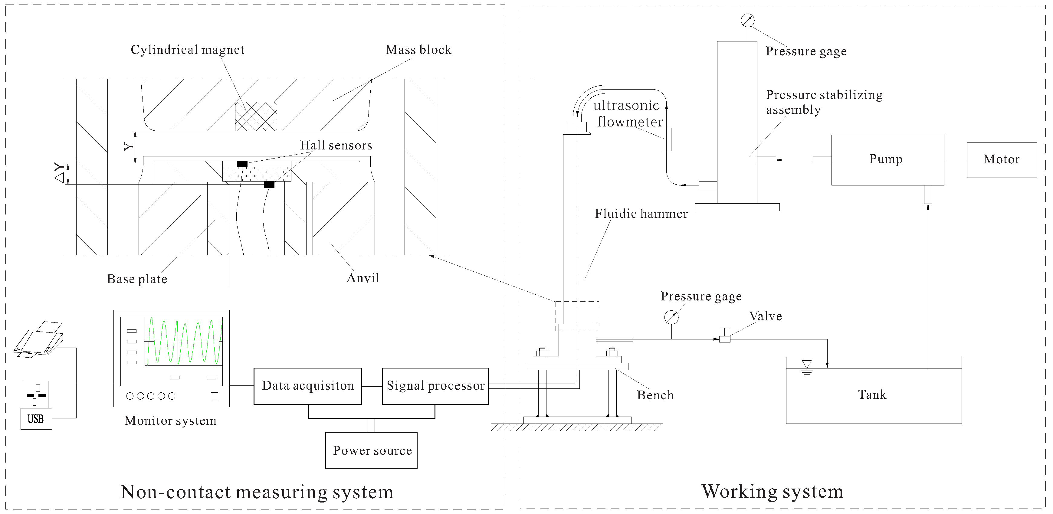
4.3. Experimental Validation

In order to verify the accuracy and reliability of the simulation results obtained by the CFD analysis, experimental tests were conducted on the SC-86H experimental prototype (Case 1). As shown in Figure 11, the tested fluidic hammer was driven by a high pressure triplex pump which supplied clean water to it. The flow rate of the feed water was measured by an ultrasonic flow meter and was adjusted by changing the speed of the electric motor, which was the power source of the triplex pump whose speed can be varied by an inverter. A pressure-stabilizing cylinder was used to reduce the fluctuation of flow rate. Besides, a noncontact measuring system based on the Hall sensors was employed to measure the impact velocity and impact frequency of the impact body. The noncontact measuring system mainly contained a cylindrical magnet, a pair of Hall sensors and a data analysis system. The integrated Hall sensors can provide an output voltage proportional to the magnetic intensity. The cylindrical magnet was fastened to the lower end face of the mass block. Two Hall sensors with the same specifications, one above the other, were mounted in pairs on the anvil. The distance ΔY between the two Hall sensors was 1.4 mm. The cylindrical magnet moves up and down with the movement of the impact body. When the distance between the upper Hall sensor and the magnet was Y, assuming that the corresponding output voltage of the sensor was U, and when the impact body moves continuously with a distance of ΔY, then the distance between the lower Hall sensor and magnet was also Y, thus the produced corresponding output voltage of the lower sensor was also U. The moving time Δt corresponding to the distance ΔY was recorded during the movement of the impact body. As the distance of Y was small enough, the impact velocity of the impact body was approximately equal to ΔY/Δt.
Figure 12 presents the comparison of the results obtained by CFD simulation and experimental tests. It can be found that the result data obtained by CFD simulation is slightly different with that of the experimental tests, but the differences are very small and do not exceed 7%, showing considerable agreement between them. The relative error may be caused by the fact that leakage and frictional force in the working chambers was ignored in the numerical calculation, and as the value of ΔY cannot be infinitely small, the measurement of impact velocity was an approximation.

5. Conclusions

The bistable fluidic oscillators are well known for their usual symmetric planar form, with the relaxation bistable oscillator and the negative feedback bistable oscillator. Less known in the output-fed bistable version, as its jet-switching mechanism is much more complex, depending on the load characteristics downstream from its output channels. This paper describes successful application of this type of fluidic oscillator developed for the control of an impact body in a DTH tool. The output-fed bistable fluidic oscillator—the flow modulation being a switching between two regimes—poses substantial applicability of reciprocating movement in adapting intelligent processing facilities.
The present paper concentrates on the performance study of a fluidic hammer controlled by an output-fed bistable fluidic oscillator. It can be concluded that the parameters of the impact body have a significant impact on the performance of the fluidic hammer, in terms of single-impact energy and output power. Pressure recovery and flow recovery were used to describe the internal flow behavior of the fluidic hammer, and were found to be closely related to the performance of the fluidic hammer. Besides, considering the various limitations and simplifications of the computational models, the agreement between the numerical and the experimental data is quite good. Thus, the CFD approach with dynamic mesh technique may be recommended for the future similar design of these fluidic oscillators.

Acknowledgments

The authors gratefully acknowledge the support of the Public Science and Technology Research Funds Projects of Ministry of Land and Resources of China (No. 201311112) for this work. The authors are also grateful to the reviewers for their helpful advices.

Author Contributions

Jianming Peng and Kun Bo conceived and designed the study. Xinxin Zhang, and Dong Ge performed the numerical simulations. Xinxin Zhang, Dong Ge and Dongyu Wu conducted the experiments. Xinxin Zhang wrote the paper. Jianming Peng, Kun Bo and Kun Yin reviewed and edited the manuscript. All authors read and approved the manuscript.

Conflicts of Interest

The authors declare no conflict of interest.

References

  1. Coanda, H. Device for Deflecting a Stream of Elastic Fluid Projected into an Elastic Fluid. U.S. Patent 2,052,869, 1 September 1936. [Google Scholar]
  2. Wang, H.; Beck, S.B.M.; Priestman, G.H.; Boucher, R.F. Fluidic pressure pulse transmitting flowmeter. Chem. Eng. Res. Des. 1997, 75, 381–391. [Google Scholar] [CrossRef]
  3. Nakayama, A.; Kuwahara, F.; Kamiya, Y. A two dimensional numerical procedure for a three dimensional internal flow through a complex passage with a small depth. Int. J. Numer. Methods Heat Fluid Flow 2005, 15, 863–871. [Google Scholar] [CrossRef]
  4. Dummer, G.W.A.; Robertson, J.M. Fluidic Components and Equipment; Pergamon: London, UK, 1968. [Google Scholar]
  5. Warren, R.W. Fluid Oscillator. U.S. Patent 3,016,066, 9 January 1962. [Google Scholar]
  6. Warren, R.W. Negative Feedback Oscillator. U.S. Patent 3,158,166, 24 November 1964. [Google Scholar]
  7. Tesař, V.; Smyk, E. Fluidic low-frequency oscillator with vortex spin-up time delay. Chem. Eng. Process. 2015, 90, 5–15. [Google Scholar] [CrossRef]
  8. Shakouchi, T. A New Fluidic Oscillator, Flowmeter, without Control Port and Feedback Loop. J. Dyn. Syst. 1989, 111, 535–539. [Google Scholar] [CrossRef]
  9. Morris, N.M. An Introduction to Fluid Logic; McGraw: New York, NY, USA, 1973. [Google Scholar]
  10. Wright, P.H. The Coanda Meter—A fluidic digital gas flowmeter. J. Phys. E 1980, 13, 433–436. [Google Scholar] [CrossRef]
  11. Jeon, M.K.; Kim, J.H.; Noh, J.; Kim, S.H.; Park, H.G.; Woo, S.I. Design and characterization of a passive recycle micromixer. J. Micromech. Microeng. 2005, 15, 346–350. [Google Scholar] [CrossRef]
  12. Lee, G.B.; Kuo, T.Y.; Wu, W.Y. A novel micromachined flow sensor using periodic flapping motion of a planar jet impinging on a V-shaped plate. Exp. Therm. Fluid Sci. 2002, 26, 435–444. [Google Scholar] [CrossRef]
  13. Groisman, A.; Enzelberger, M.; Quake, S.R. Microfluidic memory and control devices. Science 2003, 300, 955–958. [Google Scholar] [CrossRef] [PubMed]
  14. Tesař, V. Fluidic Oscillator with Bistable Jet-Type Amplifier. EP Patent 2,554,854 A2, 6 February 2013. [Google Scholar]
  15. Tesař, V.; Peszynski, K. Strangely behaving fluidic oscillator. In Proceedings of the European Physical Journal Web of Conferences, Hradec Králové, Czech Republic, 20–23 November 2012; Volume 45.
  16. Tesař, V.; Zhong, S.; Rasheed, F. New Fluidic-Oscillator Concept for Flow-Separation Control. AIAA. J. 2015, 51, 397–405. [Google Scholar] [CrossRef]
  17. He, J.F.; Yin, K.; Peng, J.M.; Zhang, X.X.; Liu, H.; Gan, X. Design and feasibility analysis of a fluidic jet oscillator with application to horizontal directional well drilling. J. Nat. Gas Sci. Eng. 2015, 27, 1723–1731. [Google Scholar] [CrossRef]
  18. Xue, L.; Li, B.M.; Wang, Z.M.; Li, B.J. Ultrahigh-Pressure-Jet-Assisted Drilling Technique: Theory and Experiment. J. Can. Petrol. Technol. 2012, 51, 276–282. [Google Scholar] [CrossRef]
  19. Luo, Y.J.; Peng, J.M.; Sun, M.Z.; Sun, Q.; Ji, T.; Bo, K. Anice-valve-based pressure-coring system for sampling naturalhydrate-bearing sediments: Proof-of-concept laboratorystudies. J. Nat. Gas Sci. Eng. 2015, 27, 1462–1469. [Google Scholar] [CrossRef]
  20. Zhang, X.; Peng, J.; Sun, M.; Gao, Q.; Wu, D. Development of applicable ice valves for ice-valve-based pressure corer employed in offshore pressure coring of gas hydrate-bearing sediments. Chem. Eng. Res. Des. 2016, 111, 117–126. [Google Scholar] [CrossRef]
  21. Peng, J.M.; Yin, Q.L.; Li, G.L.; Liu, H.; Wang, W. The effect of actuator parameters on the critical flow velocity of a fluidic amplifier. Appl. Math. Model. 2013, 37, 7741–7751. [Google Scholar] [CrossRef]
  22. Peng, J.M.; Zhang, Q.; Li, G.L.; Chen, J.W.; Gan, X.; He, J.F. Effect of geometric parameters of the bistable fluidic amplifier in the liquid-jet hammer on its threshold flow velocity. Comput. Fluids 2013, 82, 38–49. [Google Scholar] [CrossRef]
  23. Furlan, R.; Silva, M.L.P.D.; Simoes, E.W.; Leminski, R.E.B.; Aviles, J.J.S. Visualization of internal liquid flow interactions in meso planar structures. Flow Meas. Instrum. 2006, 17, 298–302. [Google Scholar] [CrossRef]
  24. Yamamoto, K.; Hiroki, F.; Hyodo, K. Self-sustained oscillation phenomena of fluidic flowmeters. J. Vis. 1999, 1, 387–396. [Google Scholar] [CrossRef]
  25. Uzol, O.; Camci, C. Experimental and computational visualization and frequency measurements of the jet oscillation inside a fluidic oscillator. J. Vis. 2002, 5, 263–272. [Google Scholar] [CrossRef]
  26. Tesař, V.; Bandalusena, H.C.H. Bistable diverter valve in microfluidics. Exp. Fluids 2011, 50, 1225–1233. [Google Scholar] [CrossRef]
  27. Wang, C.Y.; Zou, J.; Fu, X.; Yang, H.Y. Study on hydrodynamic vibration in fluidic flowmeter. J. Zhejiang Univ. Sci. A 2007, 8, 1422–1428. [Google Scholar] [CrossRef]
  28. Khelfaoui, R.; Colin, S.; Orieux, S.; Caen, R.; Baldas, L. Numerical and experimental analysis of monostable mini- and micro-oscillators. Heat Transf. Eng. 2011, 30, 121–129. [Google Scholar] [CrossRef]
  29. Tesař, V.; Hung, C.H.; Zimmerman, W.B. No-moving-part hybrid-synthetic jet actuator. Sens. Actuator A Phys. 2006, 125, 159–169. [Google Scholar] [CrossRef]
  30. Ansys Inc. Fluent User’s Guide, Release 6.3.26; Ansys Inc.: Pittsburgh, PA, USA, 2006. [Google Scholar]
  31. Chattopadhyay, H.; Kundu, A.; Saha, B.K.; Gangopadhyay, T. Analysis of flow structure inside a spool type pressure regulating valve. Energy Convers. Manag. 2012, 53, 196–204. [Google Scholar] [CrossRef]
  32. Wu, D.Z.; Li, S.Y.; Wu, P. CFD simulation of flow-pressure characteristics of a pressure control valve for automotive fuel supply system. Energy Convers. Manag. 2015, 101, 658–665. [Google Scholar] [CrossRef]
  33. Mousavian, S.M.; Najafi, A.F. Numerical simulations of gas–liquid–solid flows in a hydrocyclone separator. Arch. Appl. Mech. 2009, 79, 395–409. [Google Scholar] [CrossRef]
  34. Fan, B.W.; Pan, J.F.; Tang, A.K.; Pa, Z.H.; Zhu, Y.J.; Xue, H. Experimental and numerical investigation of the fluid flow in a side-ported rotary engine. Energy Convers. Manag. 2015, 95, 385–397. [Google Scholar] [CrossRef]
  35. Tesař, V. Mechanism of pressure recovery in jet-type actuators. Sens. Actuator A Phys. 2009, 152, 182–191. [Google Scholar] [CrossRef]
  36. Tuomas, G. Water Powered Percussive Rock Drilling: Process Analysis, Modeling and Numerical Simulation. Ph.D.Thesis, University of Lulea Tekniska, Lulea, Sweden, 2004. [Google Scholar]
  37. Franca, L.F.P. A bit-rock interaction model for rotary-percussive drilling. Int. J. Rock Mech. Min. Sci. 2011, 48, 827–835. [Google Scholar] [CrossRef]
  38. Melamed, Y.; Kiselev, A.; Gelfgat, M.; Dreesen, D.; Blacic, J. Hydraulic hammer drilling technology: Developments and capabilities. J. Energy Resour. Technol. 2000, 122, 1–7. [Google Scholar] [CrossRef]
  39. Lehmann, F.; Reich, M. Development of alternative drive concepts for downhole hammers in deep drilling operations—A feasibility study. Oil Gas Eur. Mag. 2013, 39, 119–128. [Google Scholar]
Figure 1. Four types of the bistable fluidic oscillators. (a) Relaxation bistable oscillator; (b) negative feedback bistable oscillator; (c) resonance-channel fluidic oscillator; (d) output-fed bistable oscillator.
Applsci 06 00305 g001
Figure 2. A 3D schematic of the fluidic hammer and the output-fed bistable fluidic oscillator.
Applsci 06 00305 g002
Figure 3. Main geometric parameters of the output-fed bistable fluidic oscillator; Bs—width of the supply nozzle; Ds—depth of the supply nozzle; Bc—width of the control nozzle; S—setback of the attachment wall; ls—nozzle-to-splitter distance; lv—vent-to-splitter distance; R1—radius of concave arc of the splitter; R2—radius of convex arc of the splitter; α —the divergence angle of the attachment wall.
Applsci 06 00305 g003
Figure 4. A typical 3D grid model of flow domain and the boundary condition types.
Applsci 06 00305 g004
Figure 5. A schematic circuit diagram for the fluidic hammer.(S—Inlet of supply nozzle, C—Control nozzle, V—Vent, O—Output channel, Ps—Pressure drop between supply nozzle and vent, Po—Pressure drop between output channel and vent, Qs—Flow rate at the inlet of supply nozzle, Qo—Flow rate at the output channel, u—Mean flow velocity in the supply nozzle, v—Moving velocity of the impact body, As—Sectional area of the supply nozzle, Ap—Action area of the piston, Dp—Diameter of the piston, Dr—Diameter of the piston rod, m—Mass of the impact body, L—Stroke of the impact body).
Applsci 06 00305 g005
Figure 6. The pressure recovery vs flow recovery dependences obtained at different Reynolds numbersin the forward movement of the impact body.
Applsci 06 00305 g006
Figure 7. Variations of single-impact energy E, impact frequency f, and output power P versus diameter of the piston Dp.
Applsci 06 00305 g007
Figure 8. Variations of E, f and P versus diameter of the piston rod Dr.
Applsci 06 00305 g008
Figure 9. Variations of E, f and P versus mass of the impact body m.
Applsci 06 00305 g009
Figure 10. Variations of E, f and P versus stroke of the impact body L.
Applsci 06 00305 g010
Figure 11. Schematic of the experimental system.
Applsci 06 00305 g011
Figure 12. Comparison of the results (single-impact energy and impact frequency) obtained by computational fluid dynamics (CFD) simulation and experimental tests (the difference is smaller than 7%).
Applsci 06 00305 g012
Table 1. The specified dimensions of the output-fed bistable fluidic oscillator.
Bs (mm)2.1
Ds6Bs
Bc0.8Bs
S0.5Bs
ls10Bs
lv0.5Bs
R11Bs
R21.5Bs
α 24°
Table 2. The values of parameters of the impact body investigated in the current study.
Case No.Dp (mm)Dr (mm)m (kg)L (mm)
125144140
226144140
327144140
428144140
529144140
625164140
725184140
825204140
925224140
1025146140
1125148140
12251410140
13251412140
142514460
152514480
1625144100
1725144120

