
Comparative Study on Theoretical and Machine Learning Methods for Acquiring Compressed Liquid Densities of 1,1,1,2,3,3,3-Heptafluoropropane (R227ea) via Song and Mason Equation, Support Vector Machine, and Artificial Neural Networks


Abstract
:
1. Introduction
2. Experimental Section
2.1. Theoretical Equation of State
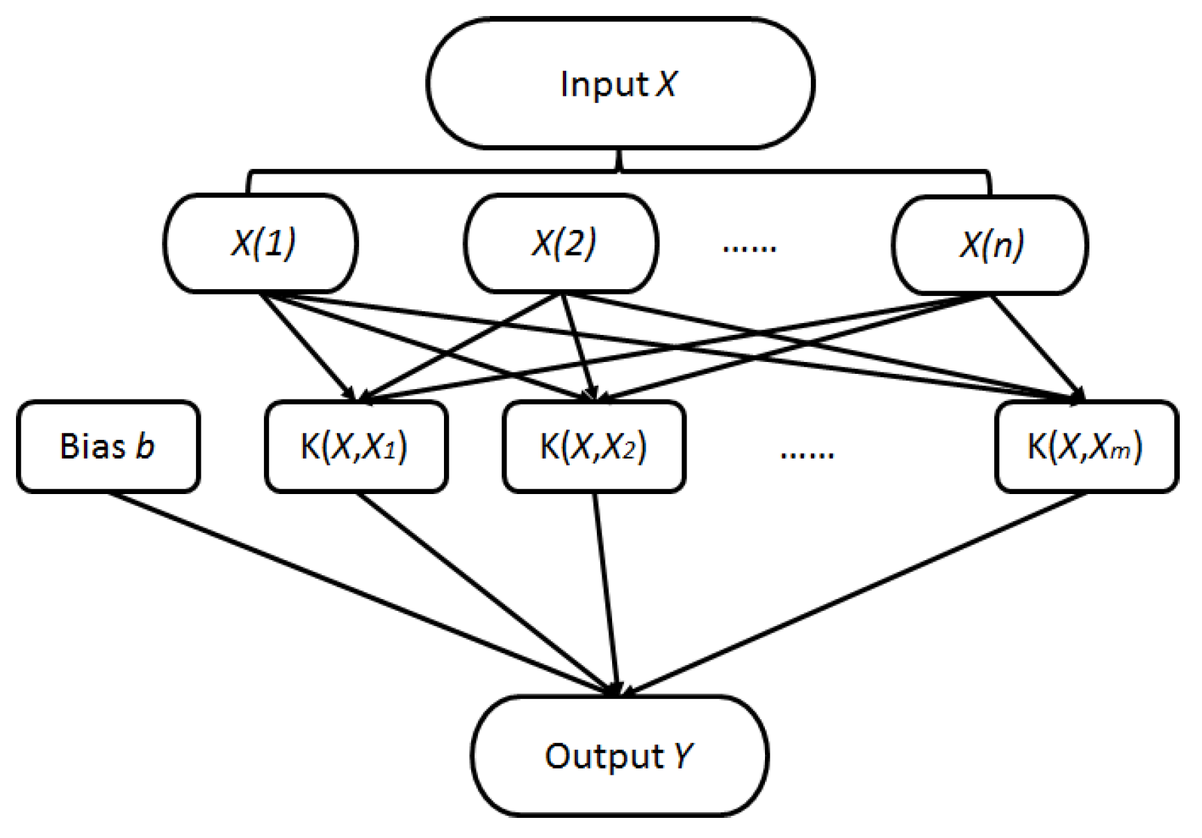
2.2. Support Vector Machine (SVM)
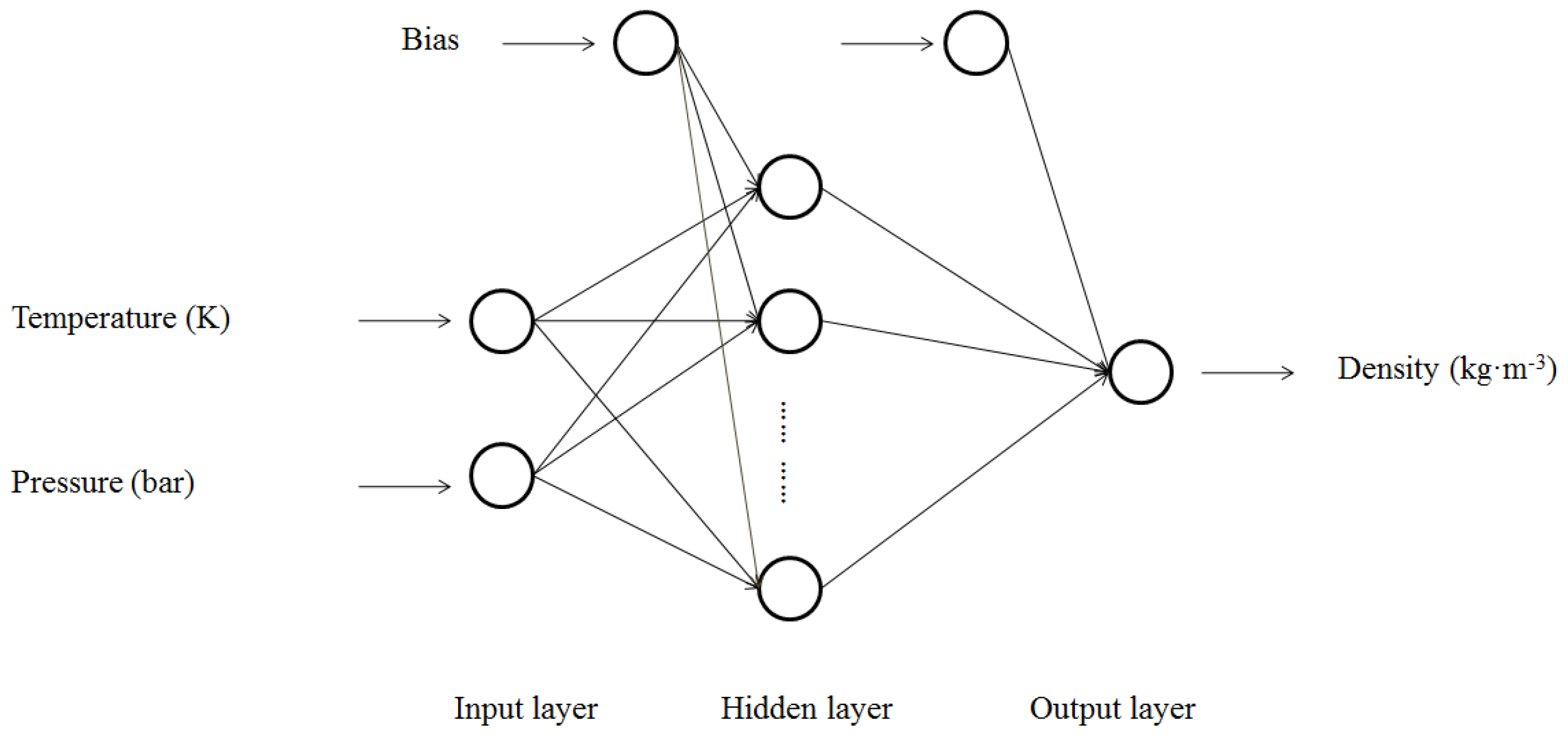
2.3. Artificial Neural Networks (ANNs)

3. Results and Discussion
3.1. Model Development
3.1.1. Theoretical Model of the Song and Mason Equation

3.1.2. Machine Learning Models

| Model Type | RMSE (for Testing) | Training Time | Prediction Accuracy |
|---|---|---|---|
| Linear Regression | 10.90 | 0:00:01 | 85.0% |
| SVM | 0.11 | 0:00:01 | 100% |
| GRNN | 1.62 | 0:00:01 | 100% |
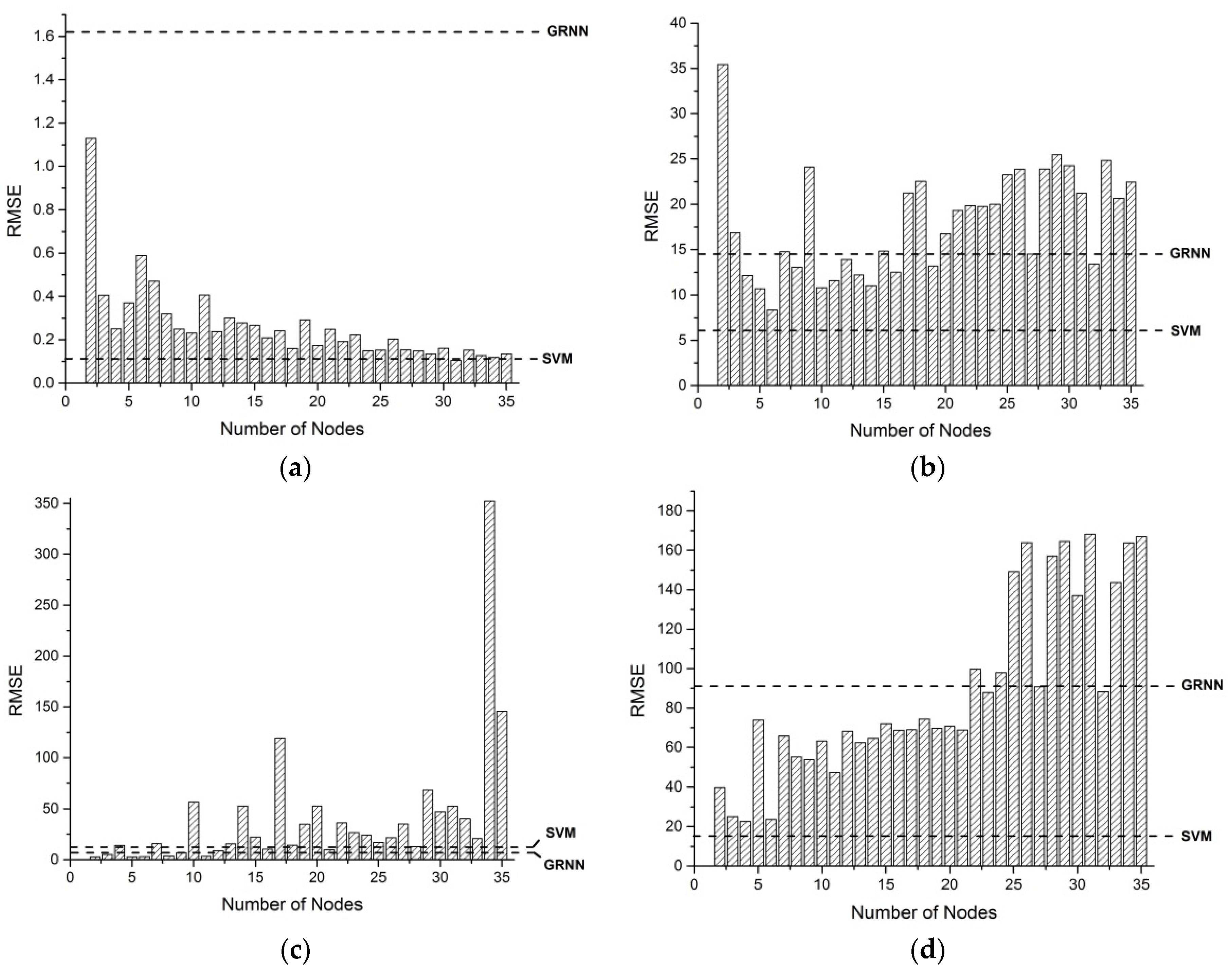
| MLFN 2 Nodes | 1.13 | 0:03:46 | 100% |
| MLFN 3 Nodes | 0.40 | 0:04:52 | 100% |
| MLFN 4 Nodes | 0.25 | 0:06:33 | 100% |
| MLFN 5 Nodes | 0.37 | 0:07:25 | 100% |
| MLFN 6 Nodes | 0.59 | 0:10:38 | 100% |
| MLFN 7 Nodes | 0.47 | 0:13:14 | 100% |
| MLFN 8 Nodes | 0.32 | 0:14:10 | 100% |
| … | … | … | … |
| MLFN 29 Nodes | 0.13 | 2:00:00 | 100% |
| MLFN 30 Nodes | 0.16 | 2:00:00 | 100% |
| MLFN 31 Nodes | 0.10 | 2:00:00 | 100% |
| MLFN 32 Nodes | 0.15 | 2:00:00 | 100% |
| MLFN 33 Nodes | 0.13 | 2:00:00 | 100% |
| MLFN 34 Nodes | 0.12 | 2:00:00 | 100% |
| MLFN 35 Nodes | 0.13 | 2:00:00 | 100% |
| Model Type | RMSE (for Testing) | Training Time | Prediction Accuracy |
|---|---|---|---|
| Linear Regression | 86.33 | 0:00:01 | 63.4% |
| SVM | 6.09 | 0:00:01 | 100% |
| GRNN | 14.77 | 0:00:02 | 96.2% |
| MLFN 2 Nodes | 35.41 | 0:02:18 | 82.7% |
| MLFN 3 Nodes | 16.84 | 0:02:55 | 96.2% |
| MLFN 4 Nodes | 12.14 | 0:03:38 | 96.2% |
| MLFN 5 Nodes | 10.67 | 0:04:33 | 96.2% |
| MLFN 6 Nodes | 8.35 | 0:04:54 | 98.1% |
| MLFN 7 Nodes | 14.77 | 0:06:06 | 96.2% |
| MLFN 8 Nodes | 13.06 | 3:19:52 | 96.2% |
| … | … | … | … |
| MLFN 29 Nodes | 25.46 | 0:31:00 | 90.4% |
| MLFN 30 Nodes | 24.25 | 0:34:31 | 90.4% |
| MLFN 31 Nodes | 21.23 | 0:42:16 | 90.4% |
| MLFN 32 Nodes | 13.40 | 3:38:17 | 96.2% |
| MLFN 33 Nodes | 24.84 | 0:47:06 | 90.4% |
| MLFN 34 Nodes | 20.65 | 0:53:14 | 90.4% |
| MLFN 35 Nodes | 22.46 | 0:58:16 | 90.4% |
| Model Type | RMSE (for Testing) | Training Time | Prediction Accuracy |
|---|---|---|---|
| Linear Regression | 15.87 | 0:00:01 | 94.1% |
| SVM | 13.93 | 0:00:01 | 94.1% |
| GRNN | 9.53 | 0:00:01 | 100% |
| MLFN 2 Nodes | 2.72 | 0:01:13 | 100% |
| MLFN 3 Nodes | 5.10 | 0:01:19 | 100% |
| MLFN 4 Nodes | 14.05 | 0:01:36 | 94.1% |
| MLFN 5 Nodes | 2.77 | 0:02:25 | 100% |
| MLFN 6 Nodes | 2.85 | 0:02:31 | 100% |
| MLFN 7 Nodes | 15.72 | 0:03:15 | 94.1% |
| MLFN 8 Nodes | 3.46 | 0:03:40 | 100% |
| … | … | … | … |
| MLFN 29 Nodes | 68.34 | 0:15:03 | 82.4% |
| MLFN 30 Nodes | 47.09 | 0:17:58 | 82.4% |
| MLFN 31 Nodes | 52.60 | 0:22:01 | 82.4% |
| MLFN 32 Nodes | 40.03 | 0:27:46 | 82.4% |
| MLFN 33 Nodes | 20.69 | 0:39:27 | 94.1% |
| MLFN 34 Nodes | 352.01 | 0:56:26 | 11.8% |
| MLFN 35 Nodes | 145.61 | 5:01:57 | 11.8% |
| Model Type | RMSE (for Testing) | Training Time | Prediction Accuracy |
|---|---|---|---|
| Linear Regression | 96.42 | 0:00:01 | 93.0% |
| SVM | 15.79 | 0:00:02 | 99.2% |
| GRNN | 92.33 | 0:00:02 | 93.0% |
| MLFN 2 Nodes | 39.70 | 0:06:50 | 96.1% |
| MLFN 3 Nodes | 25.03 | 0:08:36 | 97.7% |
| MLFN 4 Nodes | 22.65 | 0:10:06 | 99.2% |
| MLFN 5 Nodes | 73.84 | 0:13:49 | 93.0% |
| MLFN 6 Nodes | 23.64 | 0:17:26 | 99.2% |
| MLFN 7 Nodes | 65.74 | 0:14:39 | 93.8% |
| MLFN 8 Nodes | 55.32 | 0:16:18 | 93.8% |
| … | … | … | … |
| MLFN 29 Nodes | 164.54 | 0:52:29 | 89.1% |
| MLFN 30 Nodes | 136.96 | 0:37:38 | 89.8% |
| MLFN 31 Nodes | 168.13 | 0:41:35 | 89.1% |
| MLFN 32 Nodes | 88.25 | 0:50:43 | 93.0% |
| MLFN 33 Nodes | 143.65 | 2:30:12 | 89.8% |
| MLFN 34 Nodes | 163.78 | 1:00:17 | 89.1% |
| MLFN 35 Nodes | 166.92 | 0:44:16 | 89.1% |
3.2. Evaluation of Models
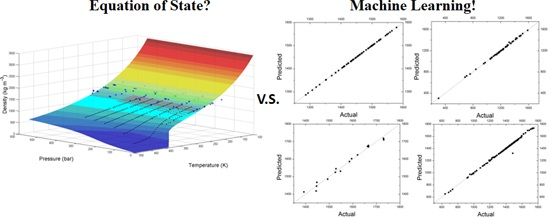
3.2.1. Comparison between Machine Learning Models and the Equation of State

| Item | RMSE in Training | RMSE in Testing |
|---|---|---|
| SVM for data provided by Fedele et al. [1] | N/A | 0.11 |
| SVM for data provided by Ihmels et al. [24] | N/A | 6.09 |
| MLFN-2 for data provided by Klomfar et al. [25] | 11.81 | 2.72 |
| SVM for all data [1,24,25] | N/A | 15.79 |
| Theoretical calculation for data provided by Fedele et al. [1] | N/A | 196.26 |
| Theoretical calculation for data provided by Ihmels et al. [24] | N/A | 372.54 |
| Theoretical calculation for data provided by Klomfar et al. [25] | N/A | 158.54 |
3.2.2. Comparison between Conventional Measurement Methods and Machine Learning
4. Conclusions
Author Contributions
Conflicts of Interest
References
- Fedele, L.; Pernechele, F.; Bobbo, S.; Scattolini, M. Compressed liquid density measurements for 1,1,1,2,3,3,3-heptafluoropropane (R227ea). J. Chem. Eng. Data 2007, 52, 1955–1959. [Google Scholar] [CrossRef]
- Garnett, T. Where are the best opportunities for reducing greenhouse gas emissions in the food system (including the food chain)? Food Policy 2011, 36, 23–23. [Google Scholar] [CrossRef]
- Gholamalizadeh, E.; Kim, M.H. Three-dimensional CFD analysis for simulating the greenhouse effect in solar chimney power plants using a two-band radiation model. Renew. Energy 2014, 63, 498–506. [Google Scholar] [CrossRef]
- Kang, S.M.; Polvani, L.M.; Fyfe, J.C.; Sigmond, M. Impact of polar ozone depletion on subtropical precipitation. Science 2011, 332, 951–954. [Google Scholar] [CrossRef] [PubMed]
- Norval, M.; Lucas, R.M.; Cullen, A.P.; de Gruijl, F.R.; Longstreth, J.; Takizawa, Y.; van der Leun, J.C. The human health effects of ozone depletion and interactions with climate change. Photochem. Photobiol. Sci. 2011, 10, 199–225. [Google Scholar] [CrossRef] [PubMed]
- Sun, J.; Reddy, A. Optimal control of building HVAC&R systems using complete simulation-based sequential quadratic programming (CSB-SQP). Build. Environ. 2005, 40, 657–669. [Google Scholar]
- T’Joen, C.; Park, Y.; Wang, Q.; Sommers, A.; Han, X.; Jacobi, A. A review on polymer heat exchangers for HVAC&R applications. Int. J. Refrig. 2009, 32, 763–779. [Google Scholar]
- Ladeinde, F.; Nearon, M.D. CFD applications in the HVAC and R industry. Ashrae J. 1997, 39, 44–48. [Google Scholar]
- Yang, Z.; Tian, T.; Wu, X.; Zhai, R.; Feng, B. Miscibility measurement and evaluation for the binary refrigerant mixture isobutane (R600a) + 1,1,1,2,3,3,3-heptafluoropropane (R227ea) with a mineral oil. J. Chem. Eng. Data 2015, 60, 1781–1786. [Google Scholar] [CrossRef]
- Coquelet, C.; Richon, D.; Hong, D.N.; Chareton, A.; Baba-Ahmed, A. Vapour-liquid equilibrium data for the difluoromethane + 1,1,1,2,3,3,3-heptafluoropropane system at temperatures from 283.20 to 343.38 K and pressures up to 4.5 MPa. Int. J. Refrig. 2003, 26, 559–565. [Google Scholar] [CrossRef]
- Fröba, A.P.; Botero, C.; Leipertz, A. Thermal diffusivity, sound speed, viscosity, and surface tension of R227ea (1,1,1,2,3,3,3-heptafluoropropane). Int. J. Thermophys. 2006, 27, 1609–1625. [Google Scholar] [CrossRef]
- Angelino, G.; Invernizzi, C. Experimental investigation on the thermal stability of some new zero ODP refrigerants. Int. J. Refrig. 2003, 26, 51–58. [Google Scholar] [CrossRef]
- Kruecke, W.; Zipfel, L. Foamed Plastic Blowing Agent; Nonflammable, Low Temperature Insulation. U.S. Patent No. 6,080,799, 27 June 2000. [Google Scholar]
- Carlos, V.; Berthold, S.; Johann, F. Molecular dynamics studies for the new refrigerant R152a with simple model potentials. Mol. Phys. Int. J. Interface Chem. Phys. 1989, 68, 1079–1093. [Google Scholar]
- Fermeglia, M.; Pricl, S. A novel approach to thermophysical properties prediction for chloro-fluoro-hydrocarbons. Fluid Phase Equilibria 1999, 166, 21–37. [Google Scholar] [CrossRef]
- Lísal, M.; Budinský, R.; Vacek, V.; Aim, K. Vapor-Liquid equilibria of alternative refrigerants by molecular dynamics simulations. Int. J. Thermophys. 1999, 20, 163–174. [Google Scholar] [CrossRef]
- Song, Y.; Mason, E.A. Equation of state for a fluid of hard convex bodies in any number of dimensions. Phys. Rev. A 1990, 41, 3121–3124. [Google Scholar] [CrossRef] [PubMed]
- Barker, J.A.; Henderson, D. Perturbation theory and equation of state for fluids. II. A successful theory of liquids. J. Chem. Phys. 1967, 47, 4714–4721. [Google Scholar] [CrossRef]
- Weeks, J.D.; Chandler, D.; Andersen, H.C. Role of repulsive forces in determining the equilibrium structure of simple liquids. J. Chem. Phys. 1971, 54, 5237–5247. [Google Scholar] [CrossRef]
- Mozaffari, F. Song and mason equation of state for refrigerants. J. Mex. Chem. Soc. 2014, 58, 235–238. [Google Scholar]
- Bottou, L. From machine learning to machine reasoning. Mach. Learn. 2014, 94, 133–149. [Google Scholar] [CrossRef]
- Domingos, P.A. Few useful things to know about machine learning. Commun. ACM 2012, 55, 78–87. [Google Scholar] [CrossRef]
- Alpaydin, E. Introduction to Machine Learning; MIT Press: Cambridge, MA, USA, 2014. [Google Scholar]
- Ihmels, E.C.; Horstmann, S.; Fischer, K.; Scalabrin, G.; Gmehling, J. Compressed liquid and supercritical densities of 1,1,1,2,3,3,3-heptafluoropropane (R227ea). Int. J. Thermophys. 2002, 23, 1571–1585. [Google Scholar] [CrossRef]
- Klomfar, J.; Hruby, J.; Sÿifner, O. measurements of the (T,p,ρ) behaviour of 1,1,1,2,3,3,3-heptafluoropropane (refrigerant R227ea) in the liquid phase. J. Chem. Thermodyn. 1994, 26, 965–970. [Google Scholar] [CrossRef]
- De Giorgi, M.G.; Campilongo, S.; Ficarella, A.; Congedo, P.M. Comparison between wind power prediction models based on wavelet decomposition with Least-Squares Support Vector Machine (LS-SVM) and Artificial Neural Network (ANN). Energies 2014, 7, 5251–5272. [Google Scholar] [CrossRef]
- De Giorgi, M.G.; Congedo, P.M.; Malvoni, M.; Laforgia, D. Error analysis of hybrid photovoltaic power forecasting models: A case study of mediterranean climate. Energy Convers. Manag. 2015, 100, 117–130. [Google Scholar] [CrossRef]
- Moon, J.W.; Jung, S.K.; Lee, Y.O.; Choi, S. Prediction performance of an artificial neural network model for the amount of cooling energy consumption in hotel rooms. Energies 2015, 8, 8226–8243. [Google Scholar] [CrossRef]
- Liu, Z.; Liu, K.; Li, H.; Zhang, X.; Jin, G.; Cheng, K. Artificial neural networks-based software for measuring heat collection rate and heat loss coefficient of water-in-glass evacuated tube solar water heaters. PLoS ONE 2015, 10, e0143624. [Google Scholar] [CrossRef] [PubMed]
- Zhang, Y.; Yang, J.; Wang, K.; Wang, Z. Wind power prediction considering nonlinear atmospheric disturbances. Energies 2015, 8, 475–489. [Google Scholar] [CrossRef]
- Leila, M.A.; Javanmardi, M.; Boushehri, A. An analytical equation of state for some liquid refrigerants. Fluid Phase Equilib. 2005, 236, 237–240. [Google Scholar] [CrossRef]
- Zhong, X.; Li, J.; Dou, H.; Deng, S.; Wang, G.; Jiang, Y.; Wang, Y.; Zhou, Z.; Wang, L.; Yan, F. Fuzzy nonlinear proximal support vector machine for land extraction based on remote sensing image. PLoS ONE 2013, 8, e69434. [Google Scholar] [CrossRef] [PubMed]
- Rebentrost, P.; Mohseni, M.; Lloyd, S. Quantum support vector machine for big data classification. Phys. Rev. Lett. 2014, 113. [Google Scholar] [CrossRef] [PubMed]
- Li, H.; Leng, W.; Zhou, Y.; Chen, F.; Xiu, Z.; Yang, D. Evaluation models for soil nutrient based on support vector machine and artificial neural networks. Sci. World J. 2014, 2014. [Google Scholar] [CrossRef] [PubMed]
- Liu, Z.; Li, H.; Zhang, X.; Jin, G.; Cheng, K. Novel method for measuring the heat collection rate and heat loss coefficient of water-in-glass evacuated tube solar water heaters based on artificial neural networks and support vector machine. Energies 2015, 8, 8814–8834. [Google Scholar] [CrossRef]
- Kim, D.W.; Lee, K.Y.; Lee, D.; Lee, K.H. A kernel-based subtractive clustering method. Pattern Recognit. Lett. 2005, 26, 879–891. [Google Scholar] [CrossRef]
- Fan, R.E.; Chang, K.W.; Hsieh, C.J.; Wang, X.R.; Lin, C.J. Liblinear: A library for large linear classification. J. Mach. Learn. Res. 2008, 9, 1871–1874. [Google Scholar]
- Guo, Q.; Liu, Y. ModEco: An integrated software package for ecological niche modeling. Ecography 2010, 33, 637–642. [Google Scholar] [CrossRef]
- Hopfield, J.J. Artificial neural networks. IEEE Circuits Devices Mag. 1988, 4, 3–10. [Google Scholar] [CrossRef]
- Yegnanarayana, B. Artificial Neural Networks; PHI Learning: New Delhi, India, 2009. [Google Scholar]
- Dayhoff, J.E.; DeLeo, J.M. Artificial neural networks. Cancer 2001, 91, 1615–1635. [Google Scholar] [CrossRef]
- Chang, C.C.; Lin, C.J. LIBSVM: A library for support vector machines. ACM Trans. Intell. Syst. Technol. 2011, 2, 389–396. [Google Scholar] [CrossRef]
- Specht, D.F. A general regression neural network. IEEE Trans. Neural Netw. 1991, 2, 568–576. [Google Scholar] [CrossRef] [PubMed]
- Tomandl, D.; Schober, A. A Modified General Regression Neural Network (MGRNN) with new, efficient training algorithms as a robust “black box”-tool for data analysis. Neural Netw. 2001, 14, 1023–1034. [Google Scholar] [CrossRef]
- Specht, D.F. The general regression neural network—Rediscovered. IEEE Trans. Neural Netw. Learn. Syst. 1993, 6, 1033–1034. [Google Scholar] [CrossRef]
- Svozil, D.; Kvasnicka, V.; Pospichal, J. Introduction to multi-layer feed-forward neural networks. Chemom. Intell. Lab. Syst. 1997, 39, 43–62. [Google Scholar] [CrossRef]
- Smits, J.; Melssen, W.; Buydens, L.; Kateman, G. Using artificial neural networks for solving chemical problems: Part I. Multi-layer feed-forward networks. Chemom. Intell. Lab. Syst. 1994, 22, 165–189. [Google Scholar] [CrossRef]
- Ilonen, J.; Kamarainen, J.K.; Lampinen, J. Differential evolution training algorithm for feed-forward neural networks. Neural Process. Lett. 2003, 17, 93–105. [Google Scholar] [CrossRef]
- Thomson, G.H.; Brobst, K.R.; Hankinson, R.W. An improved correlation for densities of compressed liquids and liquid mixtures. AICHE J. 1982, 28, 671–676. [Google Scholar] [CrossRef]
© 2016 by the authors; licensee MDPI, Basel, Switzerland. This article is an open access article distributed under the terms and conditions of the Creative Commons by Attribution (CC-BY) license (http://creativecommons.org/licenses/by/4.0/).
Share and Cite
Li, H.; Tang, X.; Wang, R.; Lin, F.; Liu, Z.; Cheng, K. Comparative Study on Theoretical and Machine Learning Methods for Acquiring Compressed Liquid Densities of 1,1,1,2,3,3,3-Heptafluoropropane (R227ea) via Song and Mason Equation, Support Vector Machine, and Artificial Neural Networks. Appl. Sci. 2016, 6, 25. https://doi.org/10.3390/app6010025
Li H, Tang X, Wang R, Lin F, Liu Z, Cheng K. Comparative Study on Theoretical and Machine Learning Methods for Acquiring Compressed Liquid Densities of 1,1,1,2,3,3,3-Heptafluoropropane (R227ea) via Song and Mason Equation, Support Vector Machine, and Artificial Neural Networks. Applied Sciences. 2016; 6(1):25. https://doi.org/10.3390/app6010025
Chicago/Turabian StyleLi, Hao, Xindong Tang, Run Wang, Fan Lin, Zhijian Liu, and Kewei Cheng. 2016. "Comparative Study on Theoretical and Machine Learning Methods for Acquiring Compressed Liquid Densities of 1,1,1,2,3,3,3-Heptafluoropropane (R227ea) via Song and Mason Equation, Support Vector Machine, and Artificial Neural Networks" Applied Sciences 6, no. 1: 25. https://doi.org/10.3390/app6010025
APA StyleLi, H., Tang, X., Wang, R., Lin, F., Liu, Z., & Cheng, K. (2016). Comparative Study on Theoretical and Machine Learning Methods for Acquiring Compressed Liquid Densities of 1,1,1,2,3,3,3-Heptafluoropropane (R227ea) via Song and Mason Equation, Support Vector Machine, and Artificial Neural Networks. Applied Sciences, 6(1), 25. https://doi.org/10.3390/app6010025