Numerical Simulation of Laminar Forced Convection of Pin-Fin Heat-Sink Array in a Channel by Using Porous Approach

Abstract

This work used a porous approach model to numerically investigate the fluid flow and heat transfer characteristics of the pin-fin heat-sink array in a rectangular channel with in-line arrangement. The air flow through the channel was laminar. The pin-fin heat sinks with various porosities and pin-fin numbers were employed. The relative center-to-center longitudinal and transverse distances between adjacent heat sinks were changed. The results indicate that the Nusselt number of various heat-sink arrays increased with decreasing the relative center-to-center transverse distance, but not varied with the relative center-to-center longitudinal distance. For the typical pin-fin heat-sink arrays, the Nusselt number changed slightly for the heat sinks with 0.358–0.556 porosity, but increased by 11.7%–24.8% when the porosity increased from 0.556 to 0.750, and then dropped obviously when the porosity exceeded 0.750. Increasing the number of pin fins continuously could increase Nusselt number. However, when the number of pin fins was large, the Nusselt number increased with the number of pin fins slowly. The present numerical simulation has been validated by the typical experiment. Finally, a semi-empirical correlation of Nusselt number for each heat sink in the heat-sink array was proposed.

1. Introduction

Since the invention of integrated circuit (IC) in 1964, the speed of computers has rapidly increased. As one IC can hold tens of electronic modules, the function of an electronic module is equivalent to a transistor or vacuum tube, so that the computer becomes smaller and more powerful. At present, the IC has evolved from early SSI (Small Scale Integrated Circuit, 10–100 modules/per unit chip) into LSI (Large Scale Integrated Circuit, 1000–10,000 modules/per unit chip), then VLSI (Very Large Scale Integrated Circuit, 100,000–1,000,000 modules/per unit chip), and finally even ULSI (Ultra Large Scale Integrated Circuit, more than a million modules/per unit chip). Such a high density package of semiconductor chip increases the heat density greatly, and the reliability or lifetime of semiconductor chip decays as the temperature rises, usually in the range of below junction temperature 100 °C. A lower temperature leads to a lower failure rate of the chip. Therefore, a good thermal control cooling design is increasingly important for high-speed computer. Multilayer PCB substrate is mounted inside general superhuge computer. Each PCB substrate is about tens of square centimeter, and carries a hundred LSIs. The cooling technique is that the finned heat sink is mounted on the LSI chip for forced air cooling. In such a configuration, there are gaps on both sides and top of the finned heat sink. A part of forced cold flow enters the internal flow channels of heat sink for cooling, and a part of cold flow leaves passing by the heat sink through the gaps. The bigger by-pass gap results in the smaller amount of the effective cold flow through the heat sink, which is disadvantageous to the overall cooling of the heat sink. Therefore, the by-pass gap and heat sink have optimal relative dimensions, so that there is maximum cooling air entering into the heat sink at fixed pumping power. This is an important topic considering actual forced air cooling.

The issue about the heat transfer characteristics of finned heat sinks without [1,2,3,4,5,6] or with bypass effect [7,8,9,10,11,12] attracts wide attention continuously. This work is to discuss putting the pin-fin heat-sink array into a rectangular channel in in-line arrangement with laminar side-bypass effect. This configuration is similar to the PCB substrate of LSI array with heat sinks inside the general supercomputer. Figure 1 shows the typical flow field of such cooling system with seven rows of heat sinks. Considering the periodical and symmetric configuration of the present system, it only shows the upper half of the single-column flow field. According to Figure 1, when the cold flow enters the heat sink array, a part of fluid exchanges heat with the heat sink, and the other part of fluid passes by the heat sink and passes through the gaps between adjacent heat-sink columns. The cold flow in the heat sink leaks out of the heat sink from side continuously under the flow-resistance effect of pin-fins, so that the downstream heat sink has less incoming cold flow. This phenomenon is especially obvious when the permeability of heat sink is low, even forming recirculating flow between downstream heat sinks. There is also a large recirculation zone behind the heat sink array. Such a change of flow field is mainly related to the flow resistance of pin-fin heat sink and the relative spacing between heat sinks, and affects the heat transfer characteristics of each heat sink significantly.

Figure 1. The upper half of the single-column flow field in seven-rows heat-sink array (the direction of pin fins is pointing the Z-axis vertical to paper surface): (a) high-permeability heat-sink array and (b) low-permeability heat-sink array.

Figure 1. The upper half of the single-column flow field in seven-rows heat-sink array (the direction of pin fins is pointing the Z-axis vertical to paper surface): (a) high-permeability heat-sink array and (b) low-permeability heat-sink array.

In the numerical simulation of heat transfer and fluid flow characteristics of finned heat sink without bypass effect, some studies regard the finned heat sink as a porous medium, using the assumption of the volume-averaging technique for computations of the porous approach model [13,14,15,16,17]. Besides, Jeng [18] used porous approach model to simulate the fluid flow and heat transfer characteristics of single square pin-fin heat sink with laminar side-bypass effect. The Brinkman-Forchheimer model was used for fluid flow and two-equation model for heat transfer. Narasimhan et al. [19,20] numerically investigated the thermal behaviors of distributed porous blocks in a channel by using a bi-disperse porous medium approach. They indicated that the Nusselt number increasing with Reynolds number changed from non-linear to linear as number of blocks increased from one to 81, with corresponding insignificant pumping power increase. Feng et al. [21] present a porous medium model for forced air convection in pin/plate-fin heat sinks subjected to non-uniform heating of an impinging jet. The forced convection is considered by employing the non-Darcy model for fluid flow and the thermal non-equilibrium model for heat transfer. They showed that the inline square pin-fin heat sink has topological advantage over the plate-fin heat sink, although the heat spreading through the plate-fins on reducing the peak temperature on the substrate is pronounced.

The current study extends the porous approach simulation method discussed in the previous study [18] to simulate the hydrodynamic and thermal behaviors of the pin-fin heat-sink array situated in a rectangular channel in an in-line arrangement with various longitudinal and transverse distances between heat sinks. The in-line pin-fin arrays of the heat sinks with various porosities and numbers of pin fins, confined uniformly within a square spreader whose side length is 67 mm, were employed. In the current study, the effects of various parameters, such as the porosity of heat sink, the number of pin fins and the relative longitudinal and transverse distances between heat sinks, on the fluid flow and heat transfer were analyzed.

2. Numerical Method

As the above-mentioned statement, this study uses the porous approach method proposed by Jeng [18] to simulate the fluid flow and heat transfer characteristics of multiple pin-fin heat sinks situated in a rectangular channel in an in-line arrangement similar to the PCB substrate of LSI array with heat sinks. In general, side-bypass and top-bypass flows exist in such issue at the same time. However, this work discusses the extreme configuration without any top-pass space above the heat-sink array. Figure 2a describes the corresponding physical configurations for the present and previous [18] studies, respectively. The previous study [18] only investigated the single pin-fin heat sink situated in a rectangular channel with laminar side-bypass flow. The originality and contribution of this work are to show the difference between single and array of pin-fin heat sink and the relevant hydrodynamic and thermal behaviors of the downstream heat sinks. Because the present study only considers the side-pass effect, it can be simplified to be two-dimensional problem with the assumption of ignoring the 3D vortex flow around the roots of pin fins. Furthermore, for the present in-line heat-sink array, each heat sink is responsible for cooling its corresponding bottom heat source. The heat flux is firstly transmitted upwards through the pin fins by heat conduction, and then transmitted to the air passing through the heat sink from the extended surface of the pin fins by heat convection. This work sets each pin-fin heat sink as a porous-medium block. Since that this work has been treated as a 2D issue, the heat dissipated from pin fins is regarded as the heat generated in the solid matrix of the porous block. Figure 2b shows the 2D configuration (x–y plane) cut from the middle of pin fins. The top view of multiple pin-fin heat sinks with in-line arrangement is presented. The center-to-center longitudinal and transverse distances (S_L^* and S_T^*) between the adjacent heat sinks are variable. Figure 2a also displays the 3D configuration of a typical pin-fin heat sink. The center-to-center longitudinal distance between the adjacent pin-fins is S_L, the center-to-center transverse distance is S_T, the number of pin-fins is n, the thickness of each square pin-fin is d, the size of pin-fin heat sink is L × L × H, and the height of the channel is H. Other assumptions are as follows: (1) the porous medium is homogenous and isotropic; (2) the fluid flow is steady state, laminar and incompressible; and (3) the thermophysical properties of the fluid and porous media do not depend on temperature. The dimensionless volume-averaged governing equations, including the Brinkman-Forchheimer model for momentum equation and two-equation model for energy equations, can be expressed as follows [18].

$$-\mathsf{\omega }=\frac{{\partial }^2\mathsf{\Psi }}{\partial X^2}+\frac{{\partial }^2\mathsf{\Psi }}{\partial Y^2}$$

(1)

$$U\frac{\partial \mathsf{\omega }}{\partial X}+V\frac{\partial \mathsf{\omega }}{\partial Y}=-\frac{{\mathsf{\epsilon }}^2}{\mathrm{Re}\cdot Da}\mathsf{\omega }-\frac{{\mathsf{\epsilon }}^2{C}_F{U}_M}{\sqrt{Da}}\mathsf{\omega }+\frac{{\mathsf{\epsilon }}^2{C}_F}{\sqrt{Da}}(U\frac{\partial U_M}{\partial Y}-V\frac{\partial U_M}{\partial X})+\frac{\mathsf{\epsilon }}{\mathrm{Re}}(\frac{{\partial }^2\mathsf{\omega }}{\partial X^2}+\frac{{\partial }^2\mathsf{\omega }}{\partial Y^2})$$

(2)

$$U\frac{\partial {\mathsf{\theta }}_f}{\partial X}+V\frac{\partial {\mathsf{\theta }}_f}{\partial Y}=\frac{N{u}_{fs}}{\mathrm{Re}\cdot \mathrm{Pr}}({\mathsf{\theta }}_s-{\mathsf{\theta }}_f)+\frac{1}{\mathrm{Re}\cdot \mathrm{Pr}}\frac{k_f^{*}}{k_f}(\frac{{\partial }^2{\mathsf{\theta }}_f}{\partial X^2}+\frac{{\partial }^2{\mathsf{\theta }}_f}{\partial Y^2})$$

(3)

$$0=N{u}_{fs}({\mathsf{\theta }}_f-{\mathsf{\theta }}_s)+\frac{k_s^{*}}{k_f}(\frac{{\partial }^2{\mathsf{\theta }}_s}{\partial X^2}+\frac{{\partial }^2{\mathsf{\theta }}_s}{\partial Y^2})+\mathsf{\delta }$$

(4)

and the relevant dimensionless parameters are as follows:

$$X=\frac{x}{H},Y=\frac{y}{H},U=\frac{u}{u_i},V=\frac{v}{u_i},\mathrm{Pr}=\frac{\mathsf{\mu }/{\mathsf{\rho }}_f}{k_f/{(\mathsf{\rho }{C}_p)}_f},Da=\frac{K}{H^2},\mathrm{Re}=\frac{{\mathsf{\rho }}_f{u}_{i}H}{\mathsf{\mu }},U_M=\frac{\sqrt{u^2+v^2}}{u_i},\mathsf{\theta }=\frac{T-T_i}{q_{w}H/k_f},N{u}_{fs}=\frac{h_{fs}{a}_{fs}{H}^2}{k_f}$$

(5)

where H is the channel (or pin-fin) height, K is the permeability; a_fs is the surface area of the fluid-solid interface per unit bulk volume of the pin-fin heat sink; h_fs is the heat transfer coefficient between the fluid stream and the solid matrix; q_w is the heat flux on the bottom of the pin-fin heat sink; ω is the vorticity, and ψ is the stream function.

$$\mathsf{\omega }=-\frac{\partial U}{\partial Y}+\frac{\partial V}{\partial X},U=\frac{\partial \mathsf{\Psi }}{\partial Y},V=-\frac{\partial \mathsf{\Psi }}{\partial X}$$

(6)

In Equations (1)–(4), C_F is the inertial coefficient; ε is the porosity of the pin-fin heat sink (i.e., the total void volume divided by the total volume occupied by the pin fins and the void volume); k_s^* is the effective conductivity of the solid matrix; and k_f^* is the effective conductivity of the fluid. Notably, in the clear fluid region, Da is set to infinity and ε to unity. In addition, Nu_fs = k_s^* = 0 and k_f^* = k_f. The δ is a function set equal to one to account for heat generation in the porous media of pin-fins and to zero elsewhere.

Figure 2. Physical configuration: (a) 3D configurations (left: present study; right: previous study [18]); and (b) 2D configuration (x–y plane) cut from the middle of fins.

Figure 2. Physical configuration: (a) 3D configurations (left: present study; right: previous study [18]); and (b) 2D configuration (x–y plane) cut from the middle of fins.

The relevant empirical coefficients in the present porous medium of pin-fins, such as K, C_F, k_s^*, k_f^* and h_fs, generally do not have universal values. This work lists the porous properties of pin-fin heat sinks studied herein in Table 1 by using the relevant empirical formula reported in the open literatures [18,22,23]. Some heat sinks in the present study are the same as those used in previous study [18]. This is for verification purposes since the single heat sink in the previous study [18] might be like the first row of heat sinks in the present study. The h_fs of the square pin-fin heat sink with uniform in-line arrangement is predicted by employing the empirical equations suggested by Kim et al. [24]:

$$h_{fs}=\frac{\mathsf{\epsilon }{k}_f}{d}\left(0.36283{{\mathrm{Re}}_d}^{0.54219}\right)\text{ for }{Re}_d<1000$$

(7)

$$h_{fs}=\frac{\mathsf{\epsilon }{k}_f}{d}\left(0.04433{{\mathrm{Re}}_d}^{0.82934}\right)\text{ for }{Re}_d\ge 1000$$

(8)

where Re_d is defined as ρ_fu_maxd/μ; u_max is the average maximum velocity between pin-fins, and d is the pin-fin thickness.

Table 1. Porous properties of pin-fin heat sinks used herein.

In-Line Square Pin-Fin Heat Sink with Uniform Distributions (SL = ST), L = 0.067 m, H = 0.0237 m
Test Specimens	Sample 1	Sample 2	Sample 3	Sample 4	Sample 5	Sample 6	Sample 7	Sample 8
d (m)	0.00596	0.00496	0.00372	0.00479	0.0067	0.00298	0.00248	0.00305
n	9 × 9	9 × 9	9 × 9	7 × 7	5 × 5	9 × 9	9 × 9	11 × 11
ε	0.358	0.556	0.750	0.750	0.750	0.84	0.889	0.75
K (m2)	4.37 × 10−8	2.40 × 10−7	1.03 × 10−6	1.63 × 10−6	2.95 × 10−6	2.13 × 10−6	3.36 × 10−6	7.03 × 10−7
CF	0.0808	0.0785	0.0451	0.0486	0.0543	0.0721	0.0862	0.0426
kf* (W·m−1·K−1)	0.0064	0.0116	0.018	0.018	0.018	0.0216	0.0231	0.018
ks* (W·m−1·K−1)	0.129	0.0694	0.036	0.036	0.036	0.0237	0.0173	0.036
afs (m2/m3)	445	381	300	241	181	251	217	360

Table 1. Porous properties of pin-fin heat sinks used herein.

In-Line Square Pin-Fin Heat Sink with Uniform Distributions (SL = ST), L = 0.067 m, H = 0.0237 m
Test Specimens	Sample 1	Sample 2	Sample 3	Sample 4	Sample 5	Sample 6	Sample 7	Sample 8
d (m)	0.00596	0.00496	0.00372	0.00479	0.0067	0.00298	0.00248	0.00305
n	9 × 9	9 × 9	9 × 9	7 × 7	5 × 5	9 × 9	9 × 9	11 × 11
ε	0.358	0.556	0.750	0.750	0.750	0.84	0.889	0.75
K (m2)	4.37 × 10−8	2.40 × 10−7	1.03 × 10−6	1.63 × 10−6	2.95 × 10−6	2.13 × 10−6	3.36 × 10−6	7.03 × 10−7
CF	0.0808	0.0785	0.0451	0.0486	0.0543	0.0721	0.0862	0.0426
kf* (W·m−1·K−1)	0.0064	0.0116	0.018	0.018	0.018	0.0216	0.0231	0.018
ks* (W·m−1·K−1)	0.129	0.0694	0.036	0.036	0.036	0.0237	0.0173	0.036
afs (m2/m3)	445	381	300	241	181	251	217	360

Figure 3a schematically depicts the numerical domain and the boundary conditions. The relevant assumptions of boundary conditions for the vorticity (ω) and the stream function (Ψ) refer Roache [25], who brilliantly discussed various boundary conditions for ω and Ψ. The fluid is assumed to enter the inlet with a uniform temperature (T_i) and a uniform velocity (u_i). The top and bottom faces are symmetric to the adjacent zones (not included in the present computational domain). The fluid phase at the outlet face is assumed to meet the zero diffusion condition since the downstream length was chosen to be sufficiently long.

This work applies the power-law developed by Patankar [26] to disperse the equations and employs the SIS (Strong Implicit Solver) algorithm proposed by Lee [27] to solve the related dispersal equations. All of the resolutions undergo the grid independence test and convergence test. The grid systems are separated into various classes to fit the physical model. The grid points, as shown in Figure 3b, are 1224 × 49–1440 × 77. The grid size falls as X_T^* and X_L^* values decrease. The X_T^*(= S_T^*/L) and X_L^*(= S_L^*/L) are the relative center-to-center longitudinal and transverse distances between the adjacent heat sinks, respectively. The iteration ends when the variables meet the criterion,

$${\displaystyle \sum }_{i,j}\left|\frac{F_{i,j}^{r+1}-F_{i,j}^r}{F_{i,j}^{r+1}}\right|\le 1\times {10}^{-5}$$

(9)

where F represents Ψ, ω or θ. The subscripts i and j refer to the i-th and the j-th grid-nodes in the X and Y directions, respectively. The superscript r indicates the r-th iteration.

Figure 3. Computational configuration (the direction of pin fins is pointing the Z-axis vertical to paper surface): (a) boundary conditions and (b) mesh (the scales of X-axis and Y-axis are different).

Figure 3. Computational configuration (the direction of pin fins is pointing the Z-axis vertical to paper surface): (a) boundary conditions and (b) mesh (the scales of X-axis and Y-axis are different).

The major parameters of heat transfer performance observed herein are the Reynolds number (Re), the dimensionless pressure drop (ΔP) and the average Nusselt number (Nu), which are defined as follows.

$$\mathrm{Re}=\frac{\mathsf{\rho }{u}_{i}H}{\mathsf{\mu }}$$

(10)

$$\Delta P=\frac{p_i-p_e}{{\mathsf{\rho }}_f{u}_i^2}={{\displaystyle \underset{L_{in}/H}{\overset{(L_{in}+L^{*})/H}{\int }}\left(\frac{1}{\mathrm{Re}Da}+\frac{C_F}{\sqrt{Da}}{U}_{M}U-\frac{1}{\mathsf{\epsilon }\mathrm{Re}}\frac{{\partial }^{2}U}{\partial X^2}+\frac{U}{{\mathsf{\epsilon }}^2}\frac{\partial U}{\partial X}\right)}}_{Y=0}dX$$

(11)

$$Nu={\displaystyle {\int }_0^L{\displaystyle {\int }_0^{L/2}N{u}_{x,y}dydx/(L^2/2)}}$$

(12)

$$\overline{Nu}={\displaystyle \sum _{i=1}^{7}N{u}_i}/7$$

(13)

where

$$N{u}_{x,y}=\frac{q_{w}H}{(T_w-T_i)k_f}=\frac{q_{w}H}{(T_s-T_i)k_f}\eta =\frac{\eta }{{\theta }_s},\mathsf{\eta }=\frac{\tanh (mH)}{mH},m=\sqrt{\frac{h_{fs}{a}_{fs}}{(1-\epsilon )k_s}}$$

(14)

The L_in is the length of channel upstream from the pin-fin heat sink.

3. Experimental Method

In order to validate the present numerical simulation, an experimental setup to investigate the smoke flow field and heat transfer characteristics of 3 × 3 pin-fin heat-sink array in a rectangular channel is built. The experimental setup displayed in Figure 4. The relevant experimental setup, procedure and heat-loss estimation are similar with those reported in the authors’ previous work [28]. The test section is made of a straightener and a rectangular channel with the 20 mm-thick Plexiglas cover and 20 mm-thick Bakelite bottom base. The configuration and dimensions of test section and positions of measured points are shown in Figure 5. In total, 9 pin-fin heat sinks are situated in the rectangular channel with X_T^*(= S_T^*/L) = 1.5 and X_L^*(= S_L^*/L) = 2.0. The Sample 5 heat sink shown in Table 1 is selected for the experiment herein. These pin-fin heat sinks are made of aluminum 6061. Each heat sink has a corresponding film heater fixed on its bottom surface. The wall heat flux supplied to each film heater from the electronic power is 0.49 W/cm² for 143 liter/min flow rate. Fifth thermocouple (Model: T-TT-30, OMEGA Engineering Inc., Stamford, CT, USA) for measuring the wall temperatures are embedded on the bottom surfaces of the center-column heat sinks. The ambient temperature and the air temperature at the channel inlet are also monitored by other thermocouples. Besides, local air velocity is measured by a hot-wire anemometer (Model: IEL VA-20, I Denshi Giken Co., Ltd., Ebina, Japan). Uncertainties in parameters are estimated by using the root-sum-square method of Moffat [29]. The experimental data obtained herein revealed that the uncertainties in the Reynolds number and the Nusselt number (as shown in Equations (10), (12) and (14)) were ±5.91% and ±6.83%, respectively.

Figure 4. Experimental setup.

Figure 4. Experimental setup.

Figure 5. Configuration and dimensions of test section and positions of measured points.

Figure 5. Configuration and dimensions of test section and positions of measured points.

4. Results and Discussion

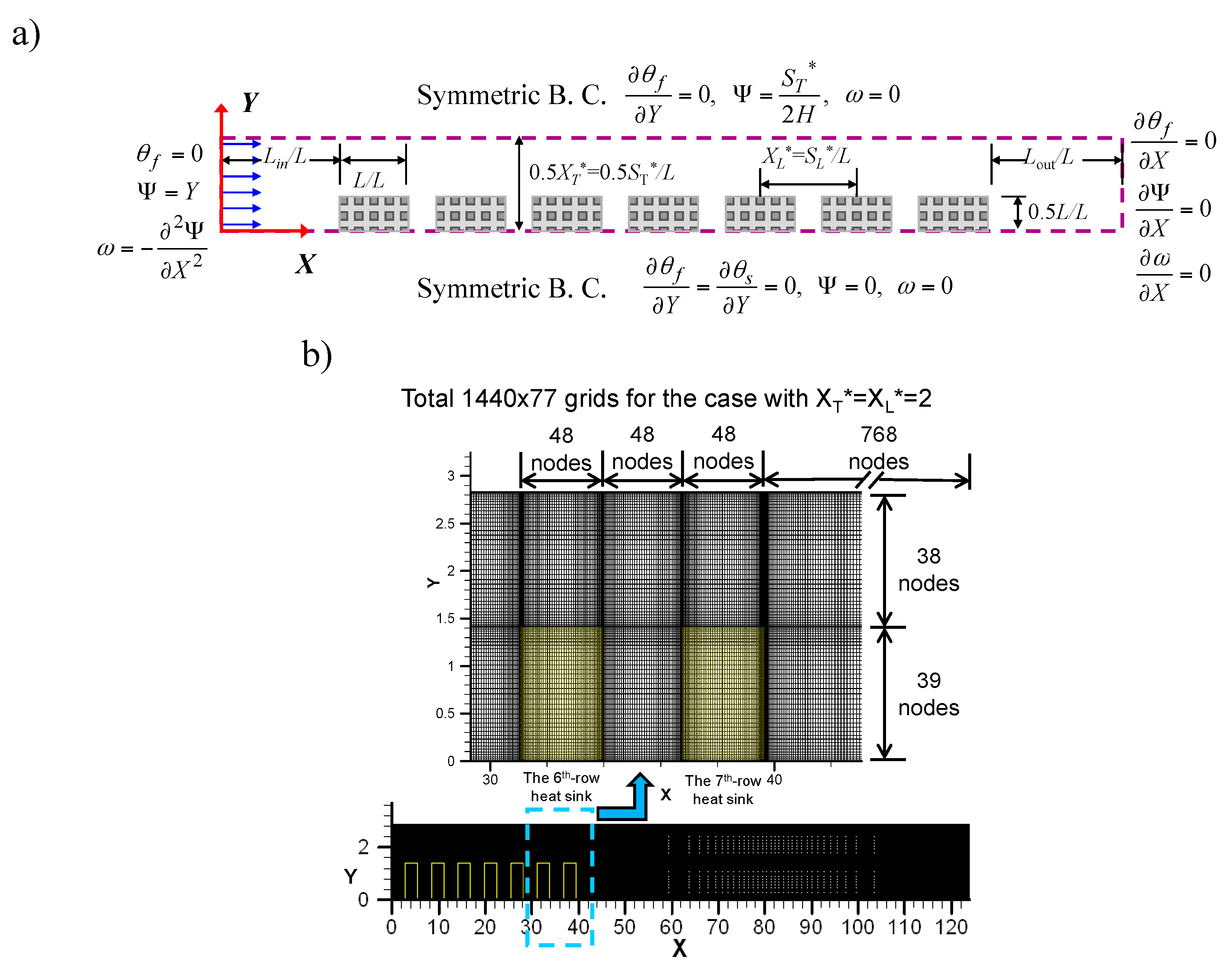
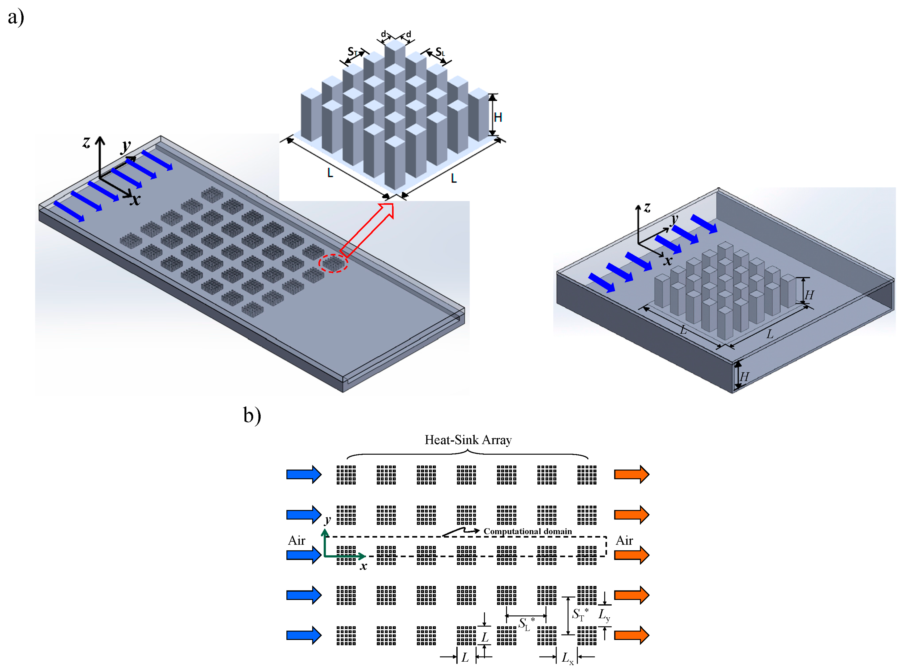
4.1. Flow Behaviors

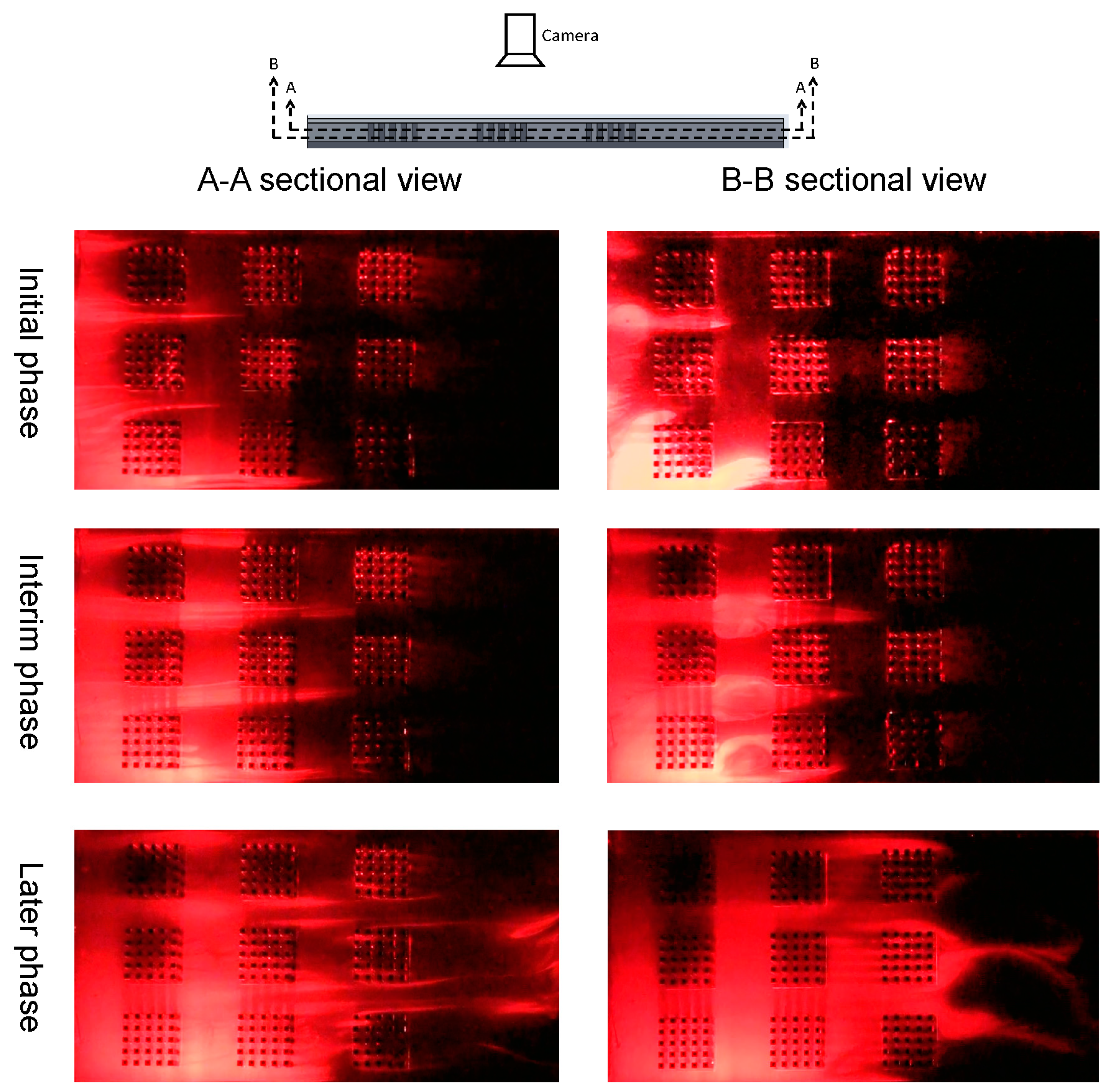
Figure 6 shows the flow visualizations of 3 × 3 pin-fin heat-sink array in a rectangular channel in the A-A and B-B sectional views of laser sheet (top-view surface tangential to inside of heat-sink array). From the visualizations of initial, interim and later phases, it can be found that the smoke flows mainly through each longitudinal passage between in-line heat sinks; minority plume goes through the heat sinks. The flow visualizations of various top views give the similar flow behaviors. Of course, the real flow pattern in the present rectangular channel with 3 × 3 pin-fin heat-sink array cannot be two-dimensional completely due to the end-wall effect. However, by comparing with the variations of fluid flow in the x and y directions, the change of fluid flow in the z direction is small and can be ignored. In other words, the present 2D simulations actually express the mean results of different cross sections along the z-axis. 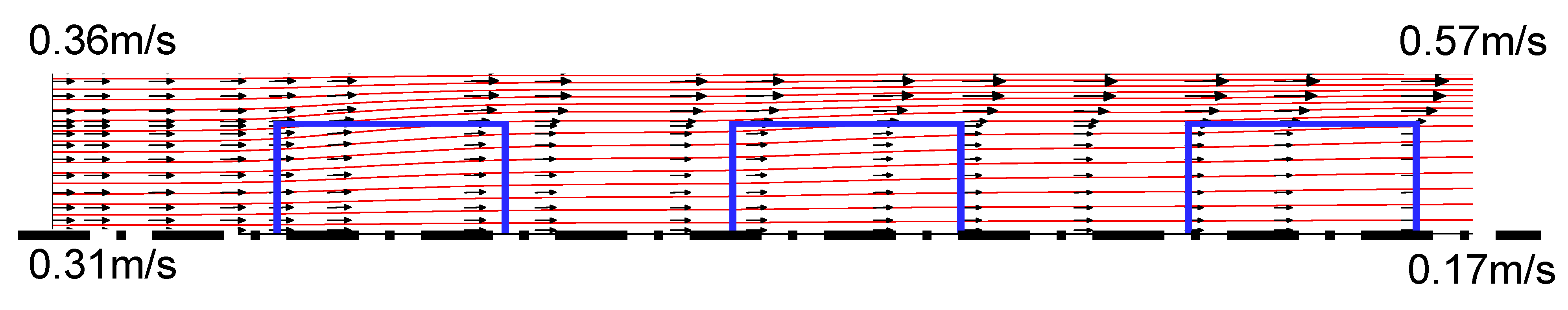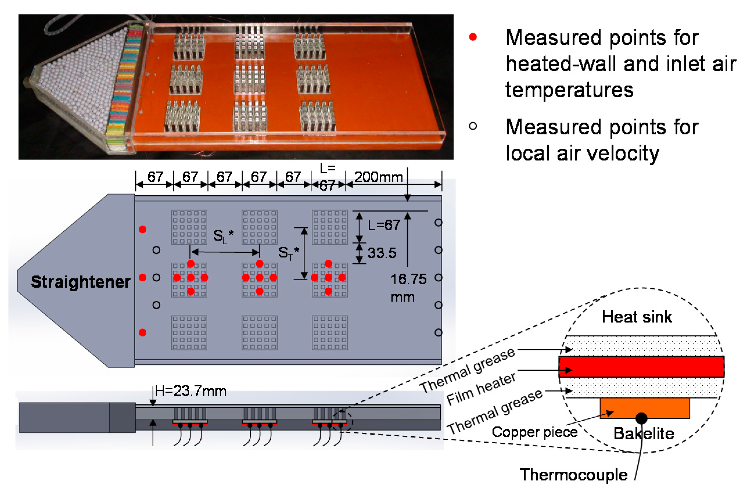Figure 7 depicts the measured values of air velocity at the inlet and outlet of the center column of 3 × 3 heat-sink array. It generally agrees to the numerical simulation.

Figure 8 shows the simulation result of streamline and velocity vector of heat-sink array in different models with Reynolds number Re = 500 and relative distances between heat sinks X_T^*(= S_T^*/L) = X_L^*(= S_L^*/L) = 1.5. It is observed that when the uniform air flows into the heat sink array, a part of air flows through the side-bypass gap between transverse adjacent heat sinks, the other part of air flows into the heat sink. In addition, due to the flow resistance, the air flow through the heat sink leaks from the side of heat sink to the side-bypass gap continuously. Therefore, the by-pass gap in more downstream location contains faster air flow; this phenomenon is more obvious in the heat sink array with bigger flow resistance. For example, the heat sink with smaller porosity or larger number of pin fins has this feature. For the heat sink array with bigger flow resistance, there are vortices formed earlier behind the last row of heat-sink array. Generally speaking, the heat-sink array with bigger flow resistance has more bypass air flow, which is adverse to heat transfer. The heat transfer of the downstream heat sink is thus worsened.

Figure 6. Flow visualization images. (Re = 52; 15 liter/min).

Figure 6. Flow visualization images. (Re = 52; 15 liter/min).

Figure 7. Measured values of air velocity at the center column of 3 × 3 heat-sink array. (Re = 500).

Figure 7. Measured values of air velocity at the center column of 3 × 3 heat-sink array. (Re = 500).

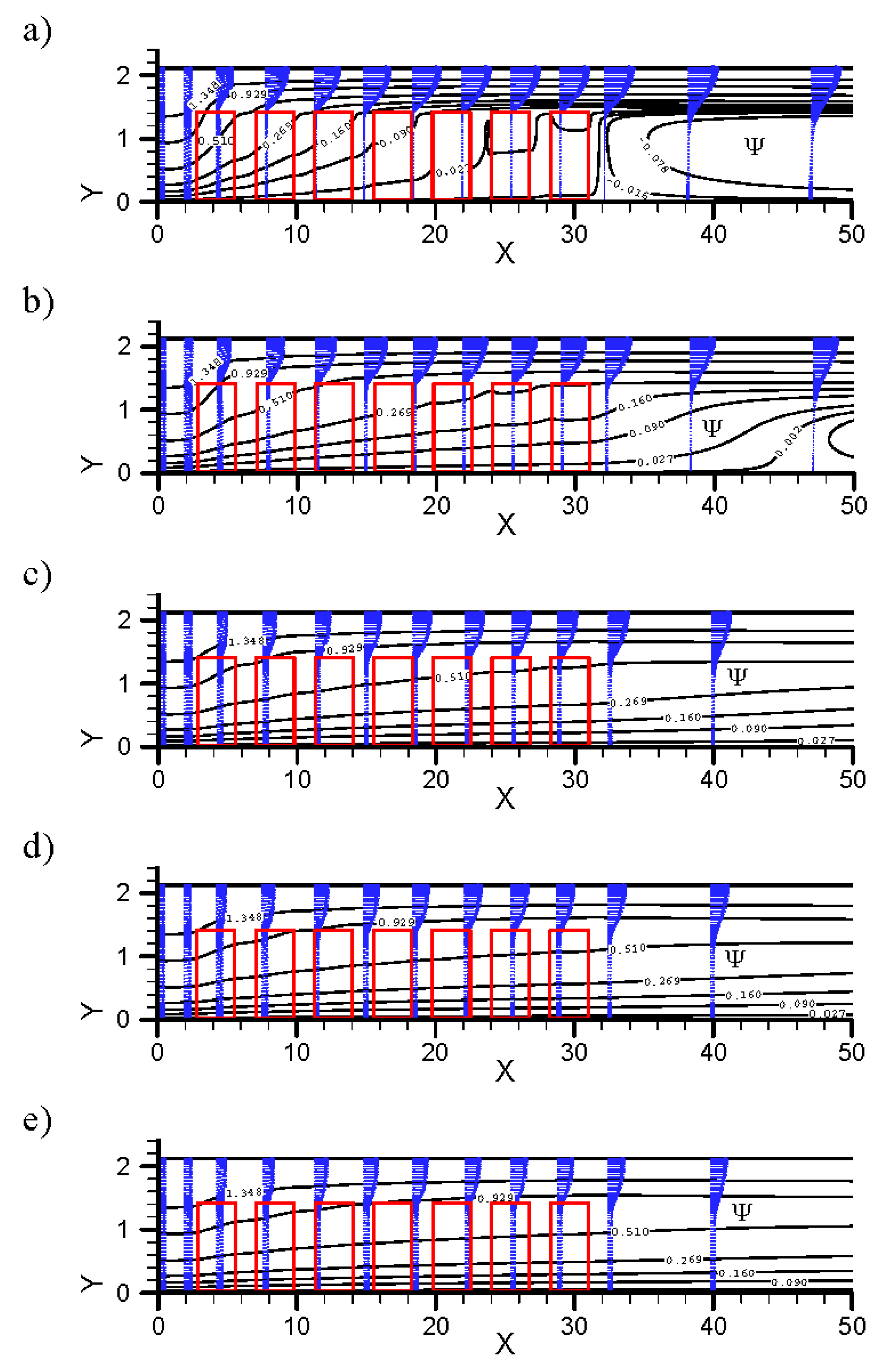
Figure 8. Streamlines and velocity vectors for various test samples with X_T^* = X_L^* = 1.5 (the scales of X-axis and Y-axis are different): (a) Sample 1; (b) Sample 2; (c) Sample 3; (d) Sample 4; and (e) Sample 5.

Figure 8. Streamlines and velocity vectors for various test samples with X_T^* = X_L^* = 1.5 (the scales of X-axis and Y-axis are different): (a) Sample 1; (b) Sample 2; (c) Sample 3; (d) Sample 4; and (e) Sample 5.

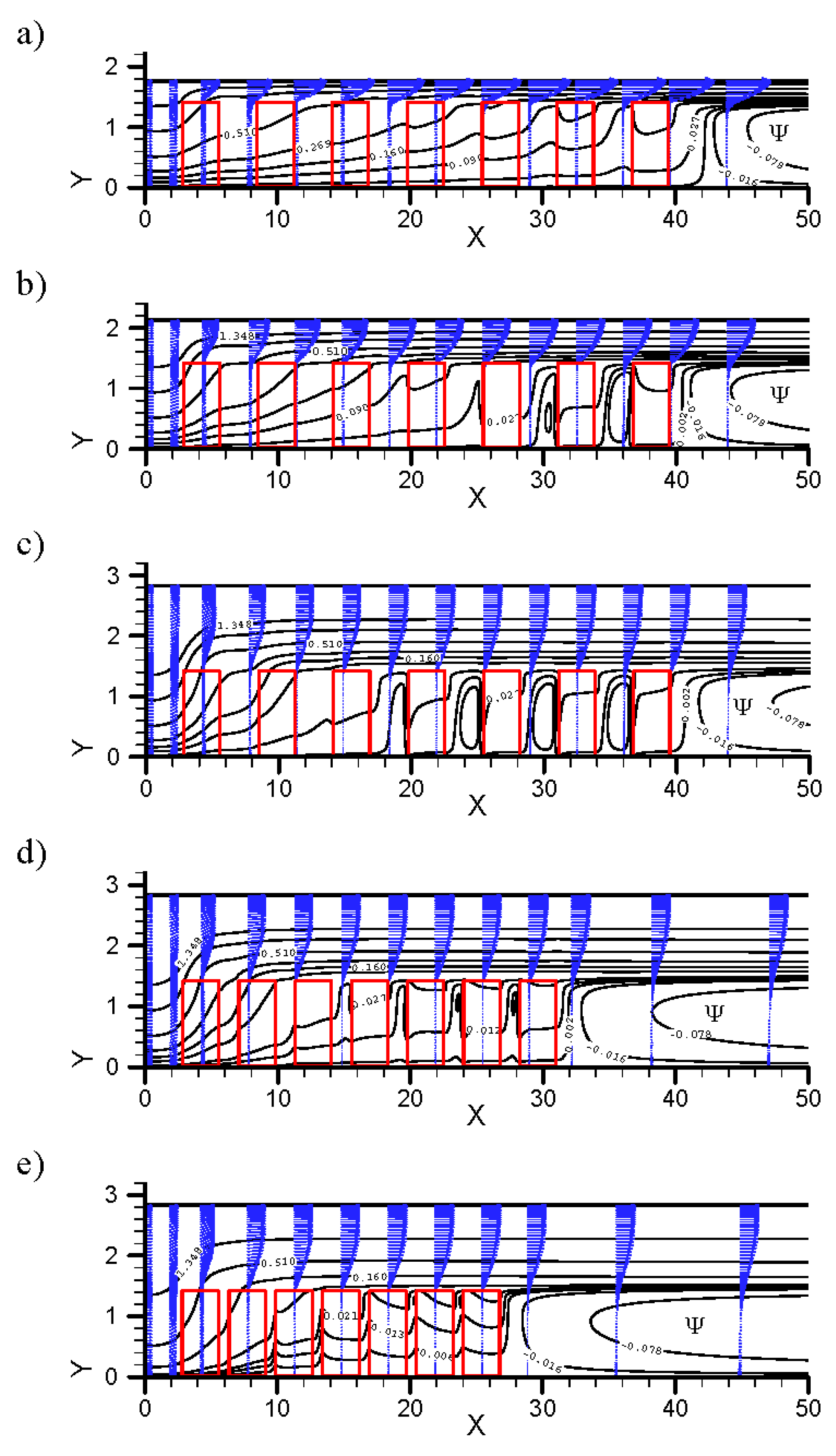
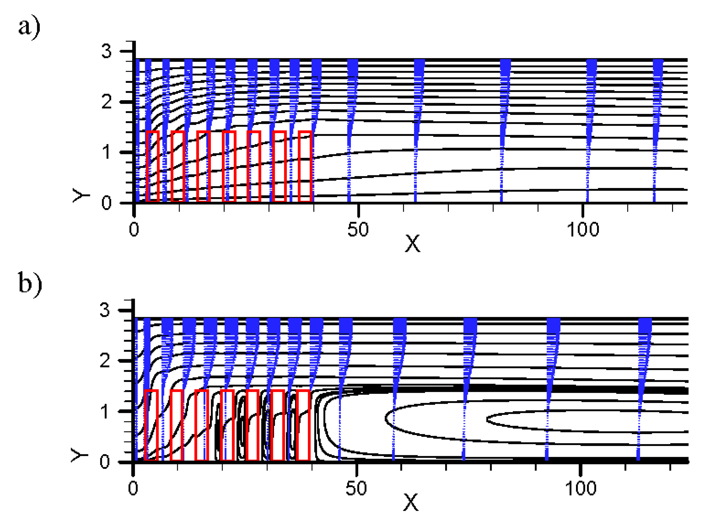
Figure 9 shows the influence of variation in the X_T^* and X_L^* values on the streamline and velocity vector taking Sample 1 heat sink array as an example. According to Figure 9a–c, when the X_L^* value is fixed at 2, a larger X_T^* represents larger relative transverse distance between heat sinks, i.e., larger lateral by-pass gap. In other words, a majority of air flow will pass through this gap, so that the air flow entering the heat sink decreases greatly (see Figure 9c). A recirculating flow is even formed between adjacent front and back rows of heat sinks in the downstream region, which is very adverse to heat transfer. According to Figure 9c–e, in the arrangement of X_T^* value fixed at 2 but different X_L^* values, the air velocity in the lateral by-pass gap is almost the same. This suggests that although the relative longitudinal distance between adjacent front and back rows of heat sinks is changed, the bypass air flow passing by the heat sink is not influenced (i.e., total air flow amount through heat sinks has not changed).

Figure 9. Streamlines and velocity vectors for test Sample 1 with various values of X_T^* and X_L^* (the scales of X-axis and Y-axis are different): (a) X_T^* = 1.25; X_L^* = 2; (b) X_T^* = 1.5; X_L^* = 2; (c) X_T^* = 2; X_L^* = 2; (d) X_T^* = 2; X_L^* = 1.5; and (e) X_T^* = 2; X_L^* = 1.25.

Figure 9. Streamlines and velocity vectors for test Sample 1 with various values of X_T^* and X_L^* (the scales of X-axis and Y-axis are different): (a) X_T^* = 1.25; X_L^* = 2; (b) X_T^* = 1.5; X_L^* = 2; (c) X_T^* = 2; X_L^* = 2; (d) X_T^* = 2; X_L^* = 1.5; and (e) X_T^* = 2; X_L^* = 1.25.

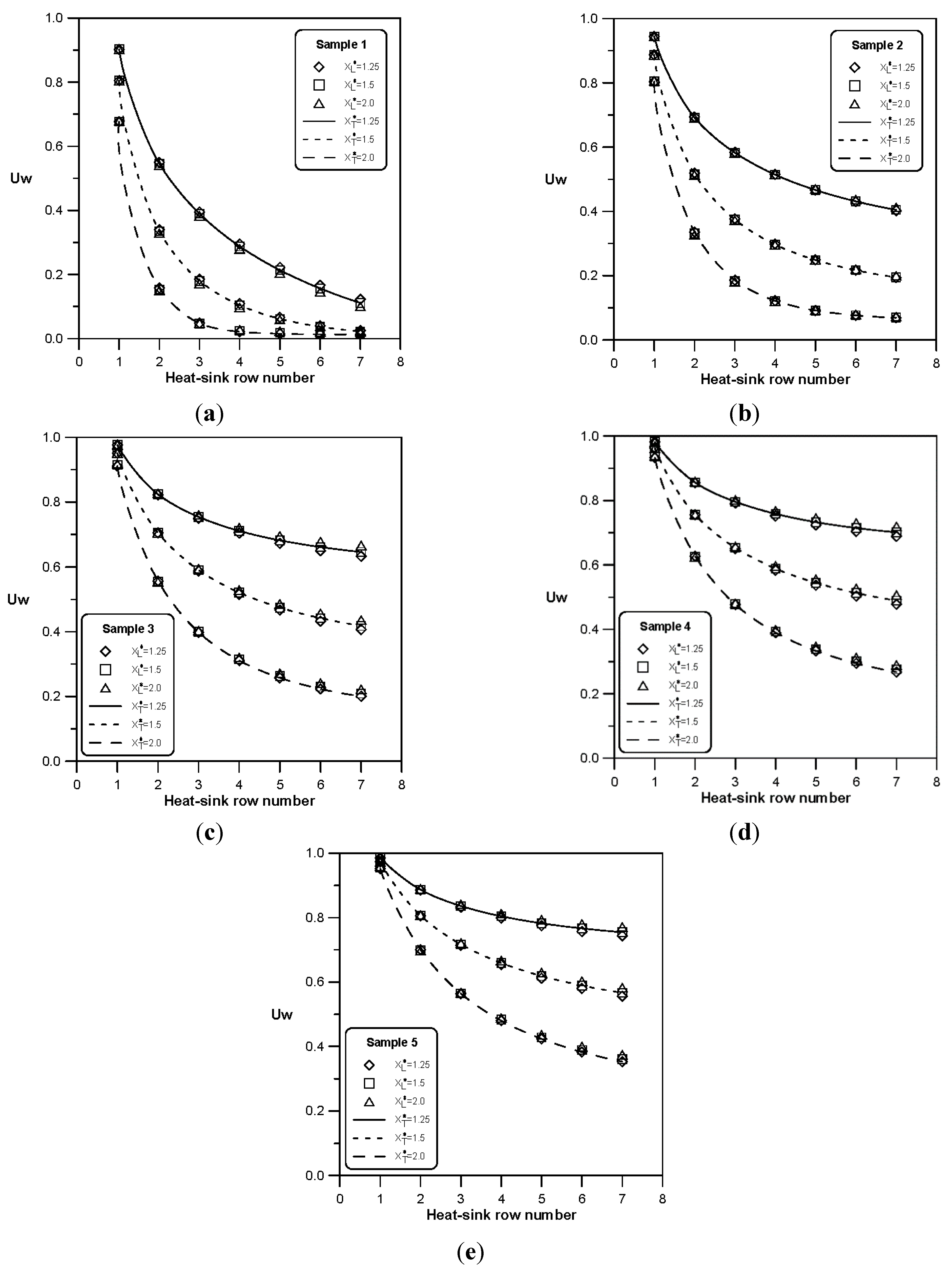
Figure 10 shows the average dimensionless velocity of air flow into windward side (U_w) of each row of heat sink array in the in-line arrangement formed of different heat sinks when Re = 500. As the flow resistance of passages between pin fins of heat sink is higher than the lateral by-pass gap between heat sinks, the air flow leaks into the by-pass gap continuously after it enters the first row of heat sink array. The leakage flow of upstream heat sink is higher than downstream heat sink. The heat sink with higher flow resistance (i.e., heat sink with lower porosity or larger number of pin fins) has less air inflow and more leakage flow. The simulation results also indicate that the influence of current relative longitudinal distance (X_L^*) between heat sinks on the air flow entering the heat sink and the leakage flow can be neglected. However, when the relative transverse distance (X_T^*) between heat sinks is large, the air flow entering the heat sink is low, and the leakage flow is high, thus reducing the forced convection heat transfer capability of heat sink array.

Figure 10. Dimensionless velocities of fluid flow through windward sides of various heat sinks: (a) Sample 1; (b) Sample 2; (c) Sample 3; (d) Sample 4; and (e) Sample 5.

Figure 10. Dimensionless velocities of fluid flow through windward sides of various heat sinks: (a) Sample 1; (b) Sample 2; (c) Sample 3; (d) Sample 4; and (e) Sample 5.

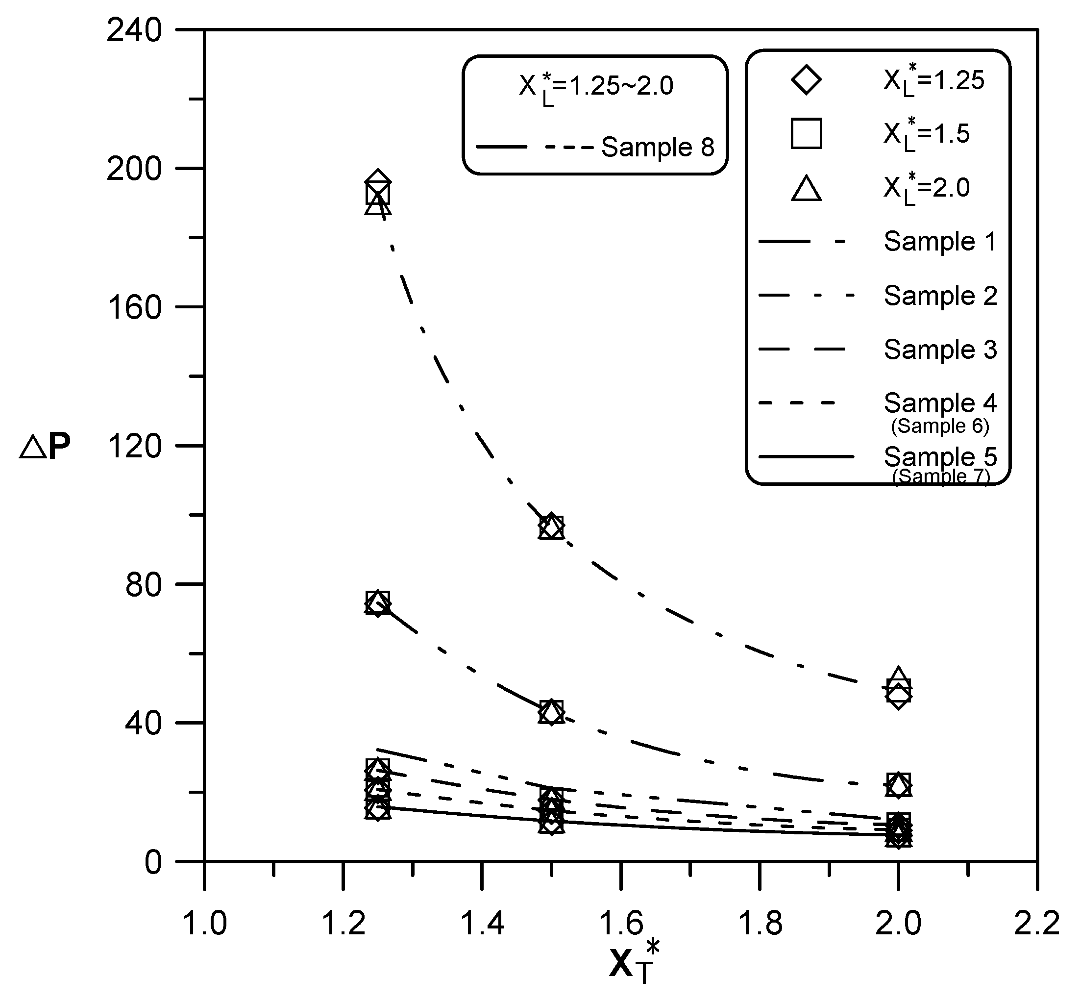
Figure 11 shows the dimensionless pressure drop when the air flow at Re = 500 passes through different heat sink arrays with different X_T^* and X_L^* values. The result indicates that changing X_L^* did not affect the dimensionless pressure drop, but increasing X_T^* would reduce dimensionless pressure drop significantly. Because an increasing X_T^* increases the air flow passing by the heat sink and reduces the air flow through the heat sink, the overall dimensionless pressure drop decreases. In addition, the array composed of heat sinks with higher flow resistance (i.e., heat sink with lower porosity or larger number of pin fins) has a larger dimensionless pressure drop.

Figure 11. Dimensionless pressure drops for different heat-sink arrays with various X_T^* and X_L^*.

Figure 11. Dimensionless pressure drops for different heat-sink arrays with various X_T^* and X_L^*.

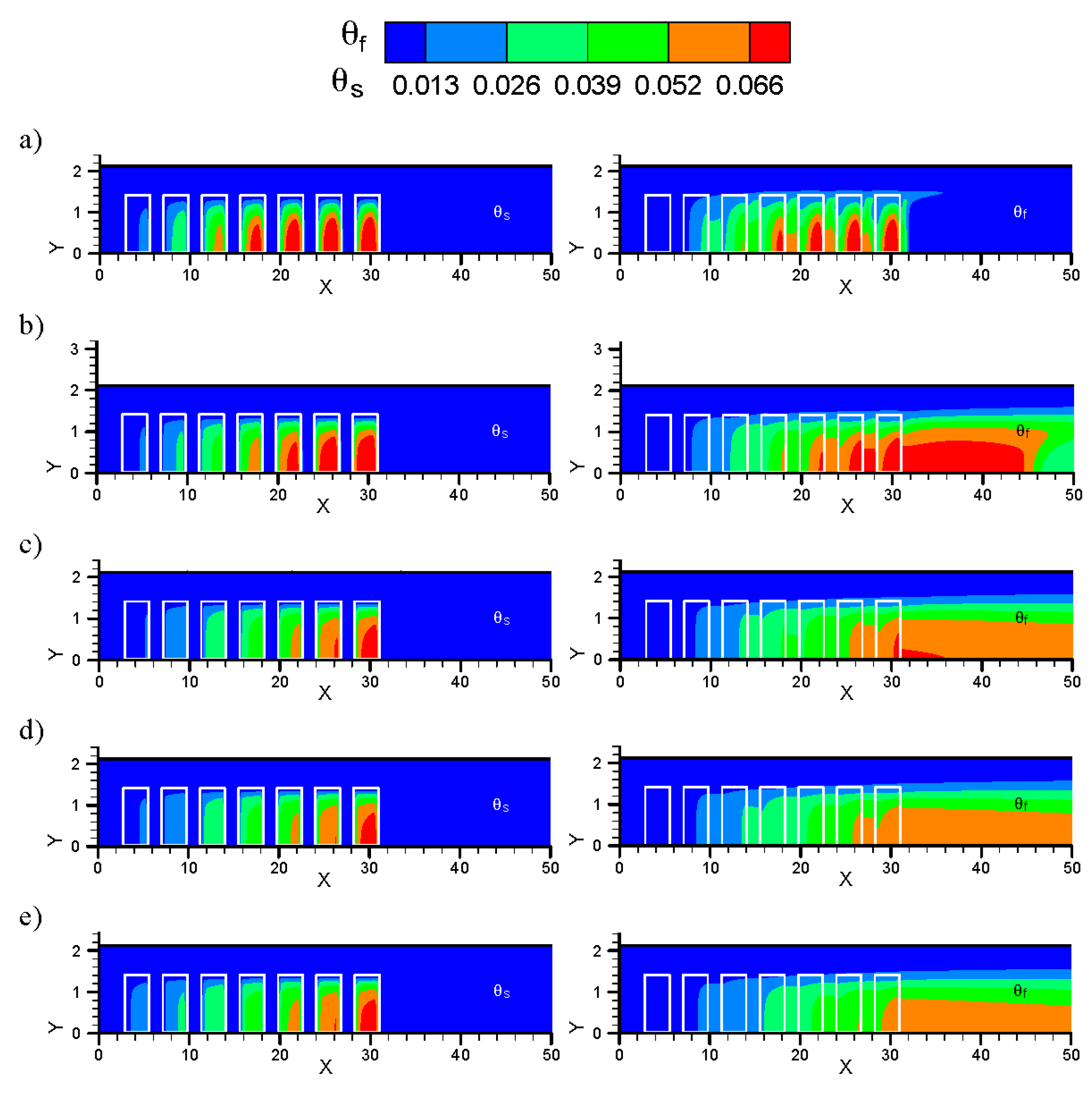
4.2. Thermal Characteristics

Figure 12 shows the dimensionless temperature contours of different heat sink arrays when Reynolds number Re = 500 and X_T^* = X_L^* = 1.5. First, the dimensionless fluid temperature and dimensionless solid temperature in the heat sink area are compared, there is significant difference, the dimensionless solid temperature is higher than the dimensionless fluid temperature, meaning in the present numerical simulation, the solid and fluid have not yet reached local thermal equilibrium. Therefore, the two-equation model meets the thermophysics in the current test system better than one-equation model. Secondly, the dimensionless solid temperature distributions of different heat sink arrays are compared (as shown in Figure 12a–c). It is observed that among the heat sink arrays with the same number of pin fins (Sample 1, Sample 2 and Sample 3), the heat sink array with higher porosity has lower overall dimensionless solid temperature, suggesting that the heat is transferred to the fluid effectively. This is because in the present cooling system, the heat considering fin efficiency radiates in each unit volume of heat sink, and then it is transmitted to the fluid by convection heat transfer. Therefore, it is basically conjugate heat transfer of thermal conduction and convection. When the porosity of heat sink is low, the upward thermal conduction capability of pin fins is better and the fin efficiency is good, thus contributing to overall heat transfer (Equation (13)). However, as shown in Figure 8, the heat sink array with lower porosity generates higher flow resistance, so that less fluid flows into the heat sink, thereby reducing the convection heat transfer of heat sink. Therefore, the heat sink Sample 1 with the smallest porosity accumulates heat in the pin-fins, so that it has the highest overall dimensionless solid temperature. The heat sink Sample 3 with the largest porosity has more cold inflow, and the dimensionless solid temperature is lower. In addition, the heat sink arrays with the same porosity (Sample 3, Sample 4 and Sample 5) are compared, as shown in Figure 12c–e. The overall dimensionless solid temperature of the Sample 3 heat sink array with more pin fins is lower than that of the Sample 4 and Sample 5 heat sink arrays with fewer pin fins, especially in the first row and the second row of heat sink array. In other words, Sample 3 with more pin fins has more heat carried away, so it is unlikely to accumulate heat. However, according to the conjugate heat transfer principle stated in Figure 12a–c, as Sample 3, Sample 4 and Sample 5 have the same porosity, they have the same upward thermal conduction capability of pin fins. However, according to Figure 10, the Sample 5 heat sink array with fewer pin fins has lower flow resistance, and it is supposed to have higher air inflow. The reason that the dimensionless solid temperature of heat sink is slightly higher than that of Sample 3 is explained below. First, the heat exchange area in unit volume of Sample 3 with more pin fins is far larger than that of Sample 4 and Sample 5 (see Table 1). This makes up the air inflow during convection heat transfer. Secondly, as shown in Equations (7) and (8), Kim et al. [24] indicated that the heat sink with smaller pin-fin diameter has larger convection heat transfer coefficient. Therefore, the dimensionless solid temperature of Sample 3 heat sink array with smaller pin-fin diameter is slightly lower than that of Sample 5.

Figure 12. Dimensionless temperature contours for various test samples with X_T^* = X_L^* = 1.5 (the scales of X-axis and Y-axis are different): (a) Sample 1; (b) Sample 2; (c) Sample 3; (d) Sample 4; and (e) Sample 5.

Figure 12. Dimensionless temperature contours for various test samples with X_T^* = X_L^* = 1.5 (the scales of X-axis and Y-axis are different): (a) Sample 1; (b) Sample 2; (c) Sample 3; (d) Sample 4; and (e) Sample 5.

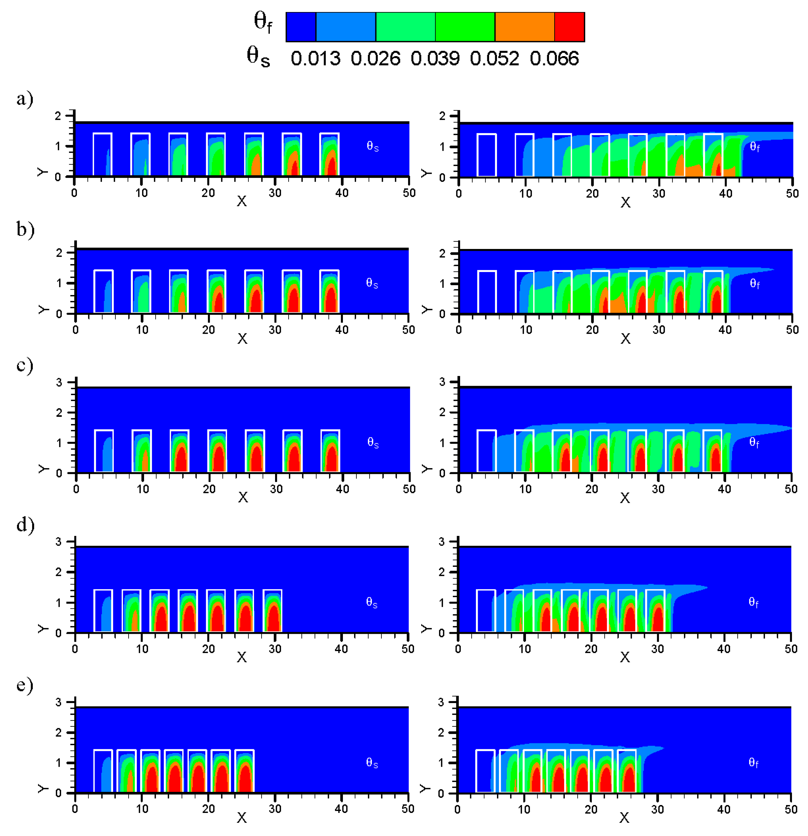
Figure 13 shows the influence of X_T^* and X_L^* on the dimensionless temperature contours taking Sample 1 heat sink array as an example when Reynolds number Re = 500. At fixed X_L^* = 2 and variable X_T^* = 1.25, 1.5 and 2, the dimensionless solid temperature of heat sink increases with X_T^*. As the increase of X_T^* amplifies the bypass effect of air flow, the air flow entering the heat sink decreases, and the heat removed decreases, so the solid part of heat sink accumulates heat and has higher temperature. Relatively, when the X_T^* is larger, as the air flowing into the heat sink is lower, the fluid has larger temperature rise though the pin fins transfer less heat to the fluid. This result is reflected in the dimensionless fluid temperature contours. At fixed X_T^* = 2 and variable X_L^* = 1.25, 1.5 and 2, the dimensionless solid temperature and dimensionless fluid temperature in the same position of various heat sinks have not varied with X_L^*, meaning X_L^* is not a sensitive parameter to the overall temperature distribution.

Figure 13. Dimensionless temperature contours for test Sample 1 with various values of X_T^* and X_L^* (the scales of X-axis and Y-axis are different): (a) X_T^* = 1.25; X_L^* = 2; (b) X_T^* = 1.5; X_L^* = 2; (c) X_T^* = 2; X_L^* = 2; (d) X_T^* = 2; X_L^* = 1.5; and (e) X_T^* = 2; X_L^* = 1.25.

Figure 13. Dimensionless temperature contours for test Sample 1 with various values of X_T^* and X_L^* (the scales of X-axis and Y-axis are different): (a) X_T^* = 1.25; X_L^* = 2; (b) X_T^* = 1.5; X_L^* = 2; (c) X_T^* = 2; X_L^* = 2; (d) X_T^* = 2; X_L^* = 1.5; and (e) X_T^* = 2; X_L^* = 1.25.

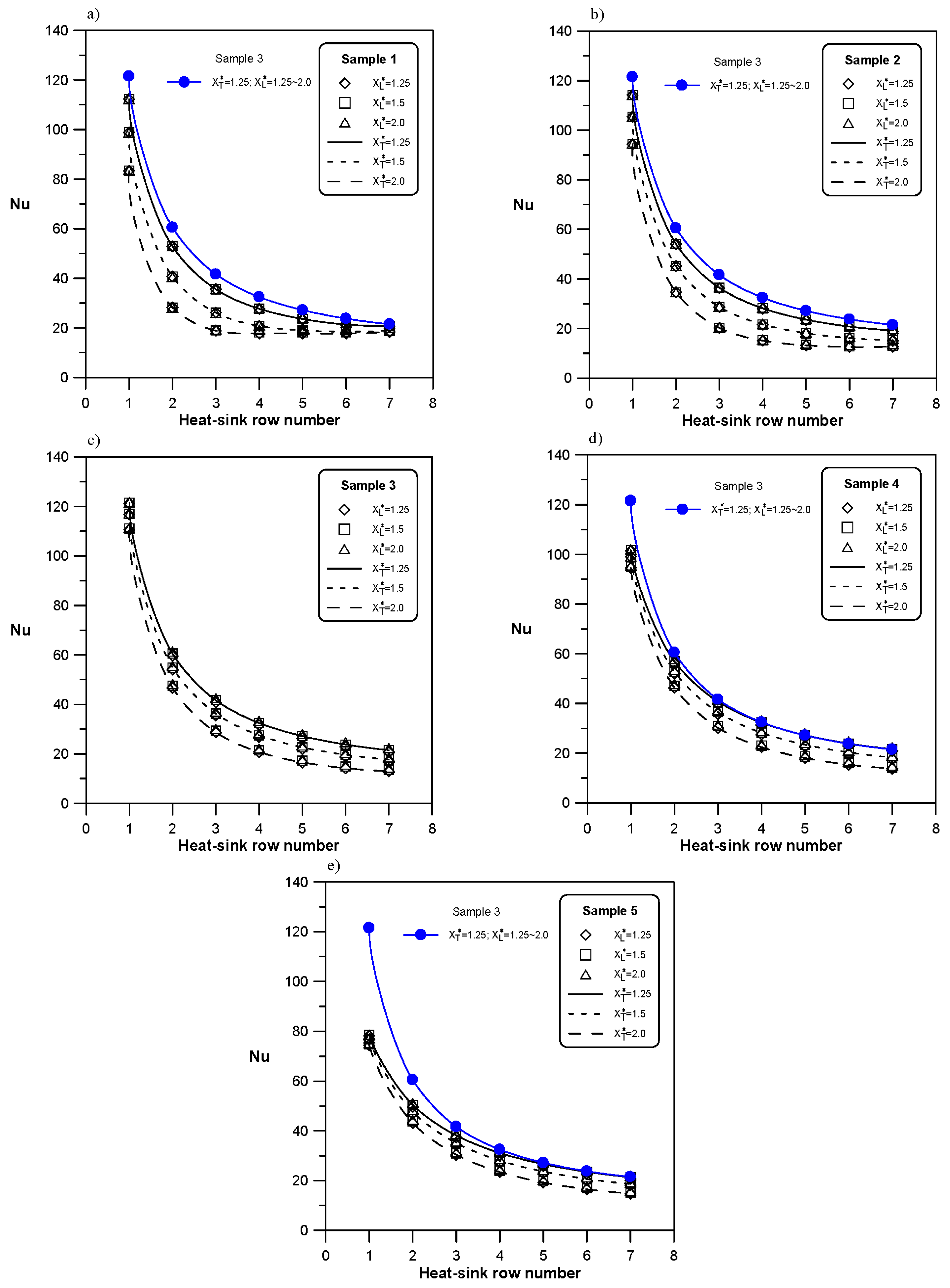
Figure 14 shows the Nusselt numbers of various rows of heat sink array at different X_T^* and X_L^* values of Samples 1–5 when Reynolds number Re = 500. The number of pin fins of Sample 3 heat sink is 9 × 9, the porosity is 0.75. This heat sink array has a higher Nusselt number among all the heat sink arrays, and the Nusselt number of various heat sink arrays increases with decreasing X_T^*, but not varies with X_L^*. This result conforms to the dimensionless temperature contours in Figure 12 and Figure 13.

Figure 14. Nusselt number distributions along the main stream direction for various heat-sink arrays: (a) Sample 1; (b) Sample 2; (c) Sample 3; (d) Sample 4; and (e) Sample 5.

Figure 14. Nusselt number distributions along the main stream direction for various heat-sink arrays: (a) Sample 1; (b) Sample 2; (c) Sample 3; (d) Sample 4; and (e) Sample 5.

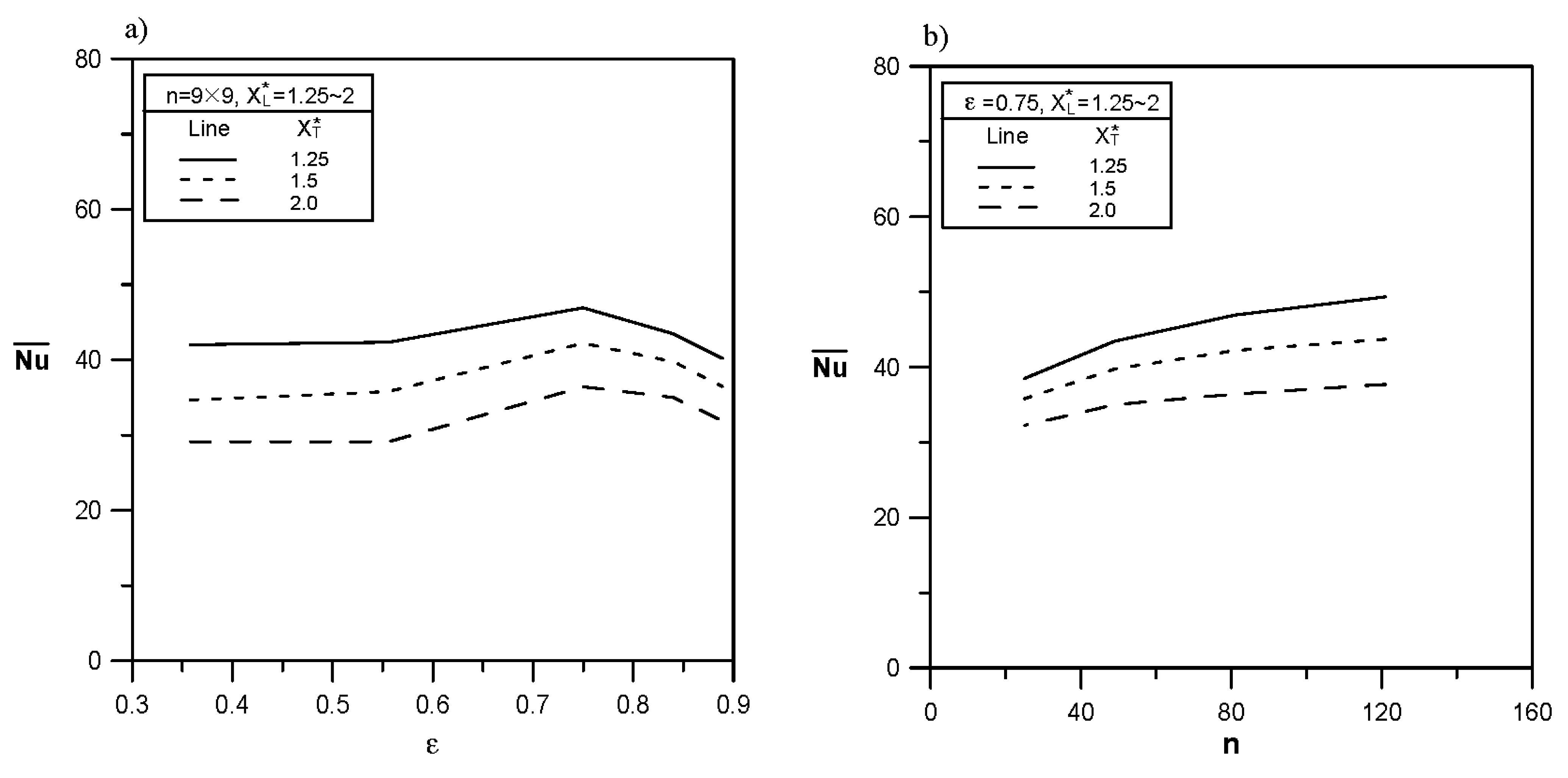
Figure 15 shows the relationship of average Nusselt number to the porosity and number of pin fins of heat sink array when Reynolds number Re = 500. In order to clarify the influences of porosity and number of pin fins on the average Nusselt number, the heat transfer characteristics of heat sink arrays with higher porosity (Sample 6 and Sample 7, see Table 1) and heat sink array with more pin fins (Sample 8, see Table 1) were also simulated. Figure 15a indicates that when the porosity of heat sink with 9 × 9 pin-fins increases from 0.358 to 0.556, the average Nusselt number changes slightly. When the porosity increases from 0.556 to 0.750, the average Nusselt number is increased significantly by 11.7% (for cases with X_T^* = 1.25)–24.8% (for cases with X_T^* = 2). However, when the porosity increases continuously from 0.750, the average Nusselt number decreases obviously. This is because the overall heat exchange area decreases with the pin diameter of pin-fin heat sink, which is adverse to convection heat transfer, and the upward thermal conduction capability of pin-fins declines, thus reducing the fin efficiency. As a result, the average Nusselt number decreases on the contrary. Figure 11b indicates that when the porosity is fixed at 0.75, increasing the number of pin fins continuously can increase the average Nusselt number. In order to keep the fixed porosity, the pin diameter must be reduced while the number of pin fins is increased; at this point, the overall heat transfer area still increases with the number of pin fins, which is advantageous to the convection heat transfer. According to empirical Equations (7) and (8) suggested by Kim et al. [24], the decrease in pin diameter increases the convection heat transfer coefficient. Therefore, the average Nusselt number increases with the number of pin fins. However, at the Reynolds number Re = 500, when the number of pin fins is large, the average Nusselt number increases with the number of pin fins slowly. The pressure drop of the heat sink array increases with the number of pin fins, thus preventing the air flow from entering the heat sink effectively for cooling.

Figure 15. Average Nusselt numbers of pin-fin heat-sink array: (a) effect of heat-sink porosity and (b) effect of pin-fin numbers.

Figure 15. Average Nusselt numbers of pin-fin heat-sink array: (a) effect of heat-sink porosity and (b) effect of pin-fin numbers.

4.3. Semi-Empirical Correlation

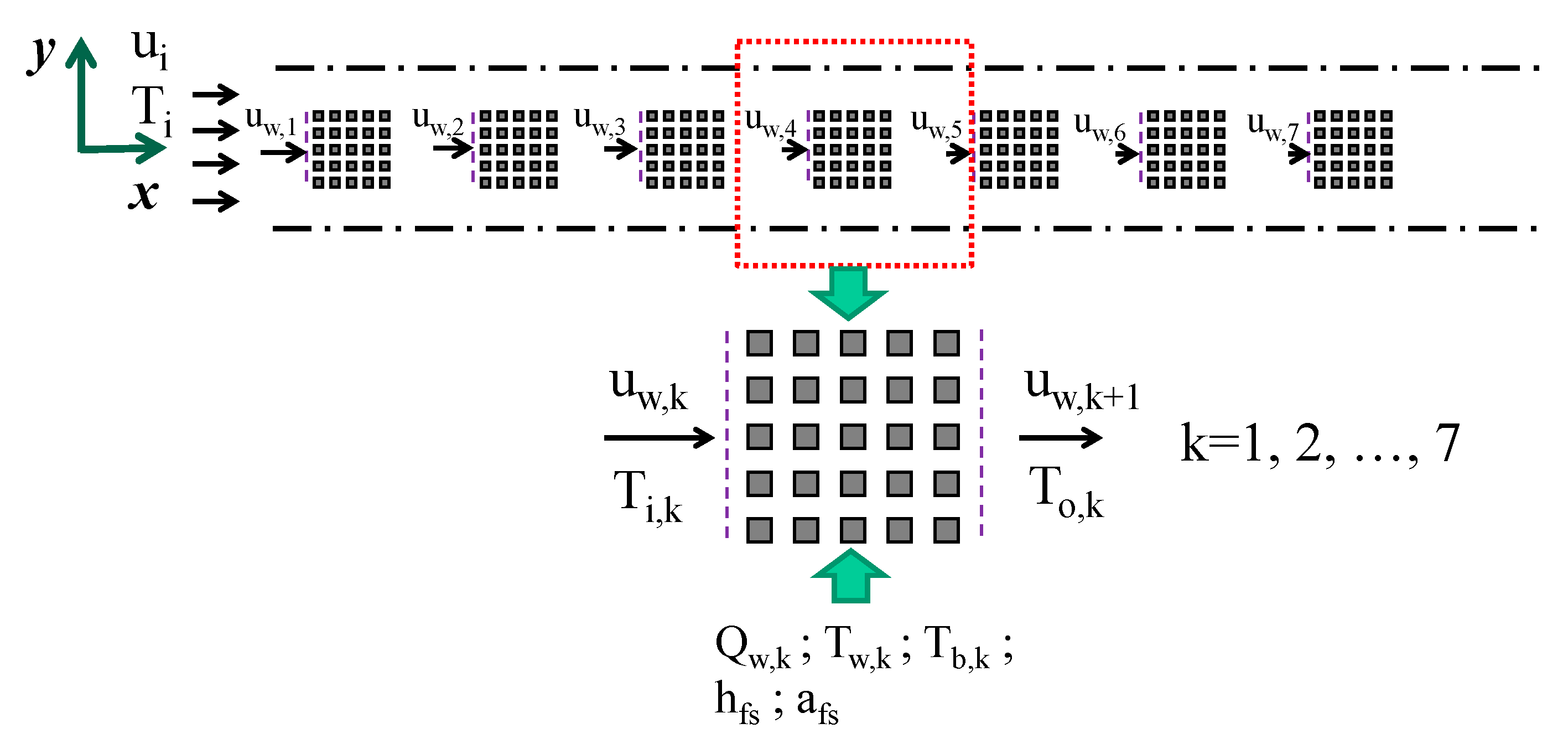
Figure 16 illustrates the energy-balance schematic diagram for the air flow heated via the heat sink in this issue. The inlet air flow has the uniform temperature (T_i) and velocity (u_i). According to Figure 10, the average velocity of air flow into windward side (u_w,k, i.e., the average velocity of flow-in air flow) of each heat sink decreases along the downward stream. In other words, a part of flow-in air continuously results in leakage air at each downward heat sink to join the bypass flow. Therefore, the energy balance for the flow-in air heated via each heat sink can be expressed as follows:

$$\rho \cdot u_i\cdot \left(\frac{U_{w,k}+U_{w,k+1}}{2}\right)\cdot H\cdot L\cdot C_p\cdot \left(T_{o,k}-T_{i,k}\right)={Q_{w,k}}^{*}$$

(15)

$$T_{b,k}=\frac{T_{o,k}+T_{i,k}}{2},U_{w,k}=\frac{u_{w,k}}{u_i}$$

(16)

where T_i,k and T_o,k are the average air temperatures at the inlet and outlet faces of the kth heat sink, respectively; T_b,k is the bulk mean temperature of the air through the kth heat sink; and Q_w,k^* is the heat transferred to the air flow through the kth heat sink. Because that the leakage-flow effect, the mean velocity of air flow through the kth heat sink is expressed as u_i(U_w,k + U_w,k+1)/2. Besides, the Q_w,k^* is less than the total heat (Q_w,k) dissipated from the kth heat sink since that the heat carried by the leakage air does not join to result in the T_o,k.

Figure 16. Energy-balance schematic diagram for the air flow heated via the heat sink.

Figure 16. Energy-balance schematic diagram for the air flow heated via the heat sink.

Equations (17) and (18) are the definitions of the average Nusselt number (Nu_i,k and Nu_b,k) of the kth heat sink separately based on T_i,1 (i.e., T_i) and T_b,k. Substitute Equations (17) and (18) into Equation (15), the relationship between Nu_i,k and Nu_b,k can be written as Equation (19).

$$N{u}_{i,k}=\frac{Q_{w,k}\cdot H}{(T_{w,k}-T_{i,k})\cdot k_f\cdot L^2}$$

(17)

$$N{u}_{b,k}=\frac{Q_{w,k}\cdot H}{(T_{w,k}-T_{b,k})\cdot k_f\cdot L^2}$$

(18)

$${N{u}_{i,k}}^{-1}={N{u}_{b,k}}^{-1}+{\displaystyle \sum _1^k\frac{{Q_{w,k}}^{*}}{Q_{w,k}}\cdot }\frac{L}{2\mathrm{Re}(\frac{U_{w,k}-U_{w,k+1}}{2})\cdot \mathrm{Pr}\cdot H}$$

(19)

Finally, a semi-empirical correlation (see Equation (20)) can be completed to be a closed form by combined with Equations (7) and (8) suggested by Kim et al. [24], the present numerical data of U_w,k plotted in Figure 10, and the assumption of Q_w,k^*/Q_w,k = U_w,k+1/U_w,k. For the present numerical simulation, C₁ and C₂ are 0.363 and 0.542, respectively (see Equation (7)).

$$\begin{array}{cc}N{u}_{b,k}& =\left(\frac{h_{fs}\cdot d}{k_f}\right)\cdot \left(\frac{H}{d}\right)\cdot \left(\frac{a_{fs}\cdot L^2\cdot H}{L^2}\right)\hfill \\ & =\left[\mathsf{\epsilon }\cdot C_1{\left(\mathrm{Re}\cdot \frac{U_{w,k}+U_{w,k+1}}{2}\cdot \frac{d}{H}\cdot \frac{S_T}{S_T-d}\right)}^{C2}\right]\cdot \left(\frac{H}{d}\right)\cdot \left(a_{fs}\cdot H\right)\hfill \end{array}$$

(20)

$$\frac{{Q_{w,k}}^{*}}{Q_{w,k}}=\frac{U_{w,k+1}}{U_{w,k}}$$

(21)

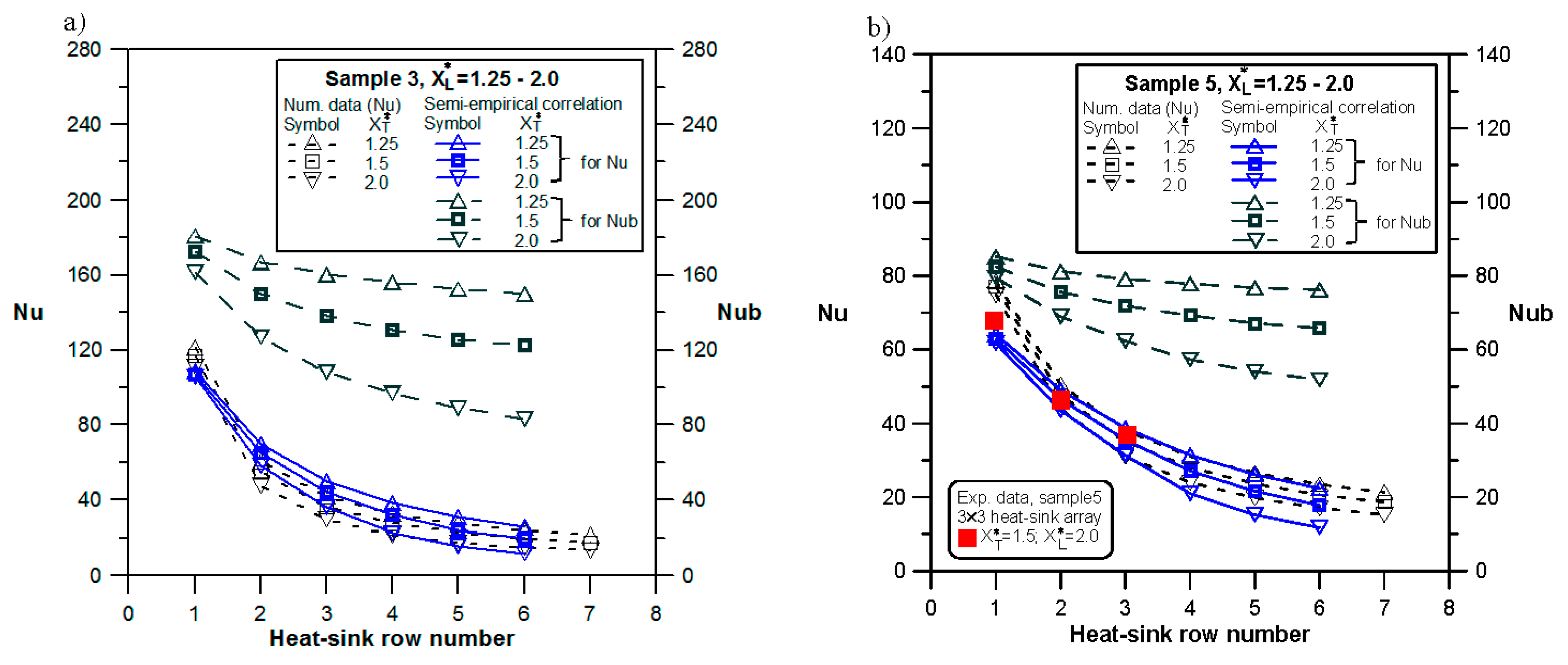
The comparison results of the present numerical Nusselt number with the semi-empirical predictions and the experimental data for Sample 3 and Sample 5 heat-sink arrays with Re = 500 are plotted in Figure 17. The predicted Nu values generally agree with those numerical data. In addition, the numerical data and the predictions of Equation (20) also agree with the typical experimental results, demonstrating the correctness of the present study.

Figure 17. Comparison results of Nusselt number with semi-empirical predictions and experimental data: (a) Sample 3 and (b) Sample 5.

Figure 17. Comparison results of Nusselt number with semi-empirical predictions and experimental data: (a) Sample 3 and (b) Sample 5.

5. Conclusions

This work successfully proposed a porous model to numerically investigate the fluid flow and heat transfer behaviors of the pin-fin heat-sink array situated in a rectangular channel in an in-line arrangement with various relative center-to-center longitudinal and transverse distances between heat sinks. The present porous approach used the Brinkman-Forchheimer model for fluid flow and two-equation model for heat transfer. The pin-fin heat sinks with various porosities and pin-fin numbers were employed. Some major conclusions are summarized as follows:

(1) By comparing with downstream heat sink, more air inflow leaks from the upstream heat sink. The heat sink with lower porosity or larger number of pin fins has less air inflow and more leakage flow. The air flow entering the heat sink is low and the leakage flow is high as the relative transverse distance (X_T^*) between heat sinks is large. However, the effect of the relative longitudinal distance (X_L^*) between heat sinks on the air flow entering the heat sink and the leakage flow is insignificant. Changing X_L^* did not affect the dimensionless pressure drop, but decreasing X_T^* would increase dimensionless pressure drop significantly. In addition, the array composed of heat sinks with lower porosity or larger number of pin fins has a larger dimensionless pressure drop.

(2) The dimensionless solid temperature is higher than the dimensionless fluid temperature, meaning the solid and fluid have not yet reached local thermal equilibrium in the present numerical simulation. Therefore, the two-equation model used for this issue is necessary. The Nusselt number of various heat-sink arrays increases with decreasing X_T^*, but does not vary with X_L^*. When the porosity of the typical heat sink increases from 0.358 to 0.556, the average Nusselt number changes slightly. However, the average Nusselt number is increased significantly by 11.7%–24.8% when the porosity increases from 0.556 to 0.750, and then drops obviously when the porosity exceeds 0.750. Besides, increasing the number of pin fins continuously can increase the average Nusselt number. However, when the number of pin fins is large, the average Nusselt number increases with the number of pin fins slowly.

(3) The present numerical simulations agree with the smoke flow visualization and heat transfer measurement of the typical experiment, proving the correctness of the present study. Finally, a semi-empirical correlation of Nusselt number for each heat sink in the present heat-sink array is proposed.