U-Shaped Transformer Image Denoising Network with Decoder-Side Pre-Fusion Calibration

Abstract

U-shaped encoder-decoder architectures are widely adopted for image denoising due to their strong capability in multi-scale modeling. However, most existing methods still rely on relatively fixed encoder-decoder feature fusion strategies, which limit effective collaboration between encoder and decoder features. To address this issue, we propose a U-shaped Transformer image denoising network with decoder-side pre-fusion calibration (UT-DPFC). Built on a U-shaped Transformer backbone, UT-DPFC inserts Structure-Detail Candidate Attention (SDCA) before encoder-decoder feature fusion at three decoding stages to calibrate decoder features, thereby providing a more reliable basis for fusion and facilitating the effective use of injected detail cues during subsequent restoration. The Transformer architecture alternately adopts Window-based Multi-Head Self-Attention (W-MSA) and Shifted Window-based Multi-Head Self-Attention (SW-MSA), together with a Locally Enhanced Feed-forward Network (LeFF), to enhance local feature modeling. SDCA generates queries from the current decoder features and performs content-adaptive retrieval and aggregation over a complementary key-value candidate pool composed of Multi-Scale Region Candidates (MSRC) and Multi-Receptive-Field Pixel Candidates (MRPC), thereby calibrating decoder features before fusion. Extensive experiments show that UT-DPFC achieves favorable performance on synthetic Gaussian and real-world denoising. It performs better in heavy noise and complex textures, maintaining moderate inference cost.

1. Introduction

Image denoising is a core problem in low-level vision, aiming to reconstruct a clean image from its noisy counterpart. The presence of noise often damages important visual structures, including edges and fine textures, which may further impair the reliability and precision of subsequent vision tasks such as image segmentation [1] and object detection [2]. Beyond image-level degradation, recent studies on adversarial noise and visual model robustness have also shown that carefully designed perturbations can significantly affect the reliability of visual recognition models in different data modalities, such as 3D point cloud classification and video recognition [3,4,5]. These studies indicate that noise and perturbations are not only pixel-level degradation factors but also important robustness-related challenges in visual data processing. Therefore, improving the ability of denoising models to preserve structural cues and recover reliable visual details is important for both low-level restoration quality and downstream visual reliability.

Owing to its practical importance, image denoising has been extensively studied in diverse application scenarios, including remote sensing imagery [6], industrial inspection [7], and medical imaging [8]. For the commonly used synthetic additive white Gaussian noise (AWGN) model, the degradation process can be expressed as $y=x+n$, where y, x, and n represent the noisy observation, the underlying clean image, and the additive white Gaussian noise, respectively. In contrast to synthetic noise, real imaging noise is typically characterized by signal dependency and spatial heterogeneity, resulting in more complex noise statistics and making real-world image denoising substantially more challenging [9].

Traditional denoising methods mainly rely on explicit priors for similar-patch matching and weighted aggregation. Aharon et al. [10] proposed K-Singular Value Decomposition (K-SVD), which performs denoising by learning an overcomplete dictionary for sparse representation. Buades et al. [11] introduced Non-Local Means (NLM), which suppresses noise through weighted averaging based on non-local patch similarity. Dabov et al. [12] further developed Block-Matching and 3D Filtering (BM3D), which achieves effective denoising by combining block matching with collaborative filtering in the transform domain. Although these methods perform well under specific noise assumptions, they depend heavily on handcrafted priors. When applied to real-world noise and complex textures, they often require careful parameter tuning and involve considerable computational cost, making it difficult to achieve a good balance between robustness and efficiency [13].

With the rapid progress of deep learning, data-driven end-to-end frameworks have significantly promoted the development of image denoising. Zhang et al. [14] introduced the Denoising Convolutional Neural Network (DnCNN), which employs residual learning to predict noise residuals explicitly, thereby improving both training stability and denoising capability. Later, Zhang et al. [15] proposed the Fast and Flexible Denoising Convolutional Neural Network (FFDNet), which incorporates a noise level map to support conditional denoising under different noise intensities. Guo et al. [16] further developed the Convolutional Blind Denoising Network (CBDNet), which enhances robustness for real-world image denoising through a two-stage design that combines noise estimation with conditional denoising. Meanwhile, U-shaped encoder-decoder architectures have become a common design paradigm in convolutional neural network (CNN)-based image restoration and denoising [17,18], as they progressively extract contextual information through downsampling, recover fine details through upsampling, and facilitate feature propagation through skip connections [19].

In recent years, to overcome the limited ability of CNNs to model long-range dependencies, Transformers have been increasingly introduced into image restoration to enhance global interactions [20]. For example, Chen et al. [21] proposed the Image Processing Transformer (IPT), which systematically introduced pre-trained Transformers into image restoration and improved both overall performance and cross-task generalization through multi-task training. Liang et al. [22] subsequently presented the Swin Transformer for Image Restoration (SwinIR), which adopts shifted window-based self-attention to enable cross-window interactions with manageable computational cost. Building on this line of research, Transformers were further incorporated into U-shaped encoder-decoder backbones as core modeling units, giving rise to U-shaped Transformer denoising models that achieve strong denoising performance by combining hierarchical architectures with attention mechanisms [23,24,25]. However, some studies have indicated that encoder features may still contain degradation-related interference, so their simple direct fusion with decoder features may introduce implicit noise, motivating the selective modulation of encoder representations using decoder-side or contextual information to facilitate more effective detail compensation [26,27]. Nevertheless, most existing methods primarily focus on enhancing the modeling capability of encoder-decoder blocks while paying limited attention to pre-fusion feature calibration, leaving the subsequent restoration process still vulnerable to interference.

Compared with existing Transformer and attention-based denoising methods, the innovation of the proposed UT-DPFC does not lie in introducing another generic self-attention module, nor in simply enhancing skip feature modulation. Instead, we shift the focus to decoder-side pre-fusion calibration, that is, to enhance and calibrate the current decoder representations before encoder-decoder fusion. To this end, we further design a structure-detail complementary candidate pool, in which Multi-Scale Region Candidates (MSRC) provide more stable region-level structural cues and Multi-Receptive-Field Pixel Candidates (MRPC) supply richer pixel-level detail responses. Based on this candidate space, the proposed Structure-Detail Candidate Attention (SDCA) performs content-adaptive retrieval and aggregation to calibrate decoder features, enabling them to serve as a more reliable basis for the subsequent fusion and restoration process. In this work, we develop a U-shaped Transformer Image Denoising Network with Decoder-Side Pre-Fusion Calibration (UT-DPFC), where SDCA is integrated at three decoding levels to strengthen the reliability of decoder features and further improve the stability of detail reconstruction in heavy-noise and complex-texture regions.

The contributions of this paper are summarized as follows:

1.

Different from existing U-shaped Transformer denoising methods that only optimize encoder/decoder blocks or regulate encoder feature injection, we propose a decoder-side pre-fusion calibration strategy. We calibrate decoder features before fusion to enhance stability in heavy noise and complex textures, which is a distinct innovation over prior U-shaped Transformer paradigms.

2.

Different from conventional attention-based denoising designs that directly perform self-attention or cross-feature interaction on existing representations, we construct a structure-detail complementary K/V candidate pool, in which Multi-Scale Region Candidates (MSRC) provide robust region-level structural cues and Multi-Receptive-Field Pixel Candidates (MRPC) supply fine-grained detail responses, thereby supporting more stable content-adaptive retrieval.

3.

We propose the Structure-Detail Candidate Attention (SDCA) module, in which pixel-wise queries generated from the current decoder features retrieve and aggregate information from the candidate pool to calibrate decoder representations before skip fusion. This design further shifts the role of attention from generic feature interaction toward decoder-oriented pre-fusion calibration.

2. Related Work

2.1. U-Shaped Encoder-Decoder Architecture

This architectural paradigm was first established by U-Net [19] and has been widely adopted in image denoising due to its effectiveness in multi-scale modeling and detail recovery through skip connections. Some methods build upon U-shaped multi-scale encoder-decoder architectures and improve denoising performance through iterative multi-scale transformation or residual learning [17,18]. Others further introduce window-based attention [23,24] or efficient attention [25] into U-shaped encoder-decoder backbones to enhance cross-scale modeling and detail restoration. In addition, Chen et al. [28] proposed the Nonlinear Activation Free Network (NAFNet), which adopts a simplified U-shaped restoration framework and achieves a favorable trade-off between restoration performance and computational efficiency. Lin et al. [29] proposed the Efficient All-Around Vision Mamba (EAMamba), which incorporates state space modeling into a U-shaped encoder-decoder architecture to improve high-resolution image restoration. More recently, Zhang et al. [30] developed the Frequency-aware U-shaped Transformer (FUT) with multi-spectral attention and dual-branch Transformer structures, and Huang et al. [31] proposed the Taylor expansion-guided Residual U-shaped Transformer (RUST) equipped with deformable spatial attention, both advancing the U-shaped Transformer paradigm for high-performance image denoising. However, under noisy perturbations, encoder features often contain both useful details and noise-related high-frequency responses. When directly fused with decoder features, skip features may lead to less balanced feature integration and amplify residual noise, which can interfere with stable detail restoration [32]. To alleviate this issue, existing studies have introduced selective modulation mechanisms during encoder feature injection to regulate the propagation strength of injected information and thereby improve fusion quality [26,27]. Different from recent U-shaped Transformer methods that mainly enhance backbone representation modeling, and from selective skip modulation methods that regulate encoder feature injection during fusion, our method focuses on decoder-side pre-fusion calibration. It performs content-adaptive calibration on decoder features before skip fusion, making the decoder representation itself a more reliable basis for subsequent encoder-decoder interaction.

2.2. Attention-Driven Content-Adaptive Retrieval and Aggregation

Non-local self-similarity, which essentially describes content-adaptive retrieval and aggregation across spatial locations, has long been a core guiding principle for image denoising. Non-Local Means (NLM) [11] computes non-local weights based on patch similarity and performs weighted averaging over correlated pixels across the image. Subsequent differentiable non-local modeling methods [33,34,35] further integrated this process into end-to-end learning, demonstrating that content-adaptive aggregation is effective for noise suppression. Representative methods such as Swin Transformer for Image Restoration (SwinIR) [22] enhance long-range dependency modeling with manageable computational cost by employing window-based self-attention. Unlike self-attention, which performs modeling within a homogeneous feature source, cross-attention enables information retrieval and aggregation across different feature sources. Specifically, Q are generated from one feature source, whereas K/V are provided by another, thereby enabling cross-source prior injection and complementary interaction. For example, Hu et al. [36] proposed the Dual-Stem Cross-Attentive Transformer for Image Denoising (DSCA-former), which facilitates cross-source interaction between spatial and channel features through a bidirectional Q/K/V exchange mechanism, thereby enabling alternating feature calibration. Unlike conventional self-attention or generic cross-attention designs, the proposed SDCA leverages decoder features as queries and an explicitly constructed structure-detail candidate pool as keys/values, thus reorienting attention into a decoder-side pre-fusion calibration mechanism. Here, Q represents the current decoding state, while K/V encode structure-detail candidates, enabling content-adaptive retrieval from the pool and subsequent decoder feature calibration. This design effectively addresses the limitations of fixed fusion strategies, which apply identical operations to all spatial positions and often fail to adapt to varying noise and texture distributions.

2.3. Multi-Scale Candidate Construction Strategy

Different scales and receptive fields can provide complementary information. Representative strategies mainly include pyramid pooling-based methods and dilated convolution-based methods. For example, He et al. [37] proposed Spatial Pyramid Pooling (SPP), which captures region-level information through multi-scale pooling. Chen et al. [38] further introduced Atrous Spatial Pyramid Pooling (ASPP), which expands the effective receptive field using multiple dilation rates while preserving spatial resolution. Although these methods were originally proposed for general vision tasks, their underlying principles have also provided important inspiration for image denoising. Zhao et al. [39] proposed the Pyramid Real Image Denoising Network (PRIDNet), which incorporates pyramid pooling into real-world image denoising to enhance multi-scale feature representation. Jia et al. [40] proposed the Pyramid Dilated Convolutional Neural Network (PDCNN), which extracts and fuses multi-scale contextual information by arranging dilated convolutions with different dilation rates in a pyramid structure, thereby expanding the effective receptive field while strengthening edge and texture-detail modeling. Duong et al. [41] proposed the Multi-Branch Network (MBN), which aggregates multi-scale contextual information through parallel dilated convolution branches with different dilation rates, thereby improving feature representation and denoising performance. Therefore, the role of MSRC and MRPC in our framework is not merely multi-scale feature enhancement, but the explicit construction of complementary structural and detail candidates for stable retrieval and aggregation. Multi-scale Region Candidates (MSRC) provide more robust structural candidates, whereas Multi-Receptive-Field Pixel Candidates (MRPC) provide richer detail candidates. These candidates are jointly organized into a K/V candidate pool for attention-based retrieval and aggregation, thereby supplying more reliable, complementary, structural, and detailed information for decoder-side pre-fusion calibration.

3. Methods

3.1. Method Overview

In conventional U-shaped denoising networks, decoder features are usually fused with the corresponding encoder features in a relatively direct manner. In contrast, the proposed UT-DPFC first calibrates decoder features before skip fusion. At each selected decoder stage, the current decoder feature generates pixel-wise queries, which retrieve complementary structural and detail cues from a candidate pool constructed by Multi-Scale Region Candidates (MSRC) and Multi-Receptive-Field Pixel Candidates (MRPC). The retrieved information is then injected into the decoder branch, making the calibrated decoder representation a more reliable basis for subsequent encoder-decoder fusion. This pre-fusion calibration effectively suppresses noise interference inherited from encoder features in heavy noise scenarios, making feature fusion more stable and reliable.

3.2. Network Architecture

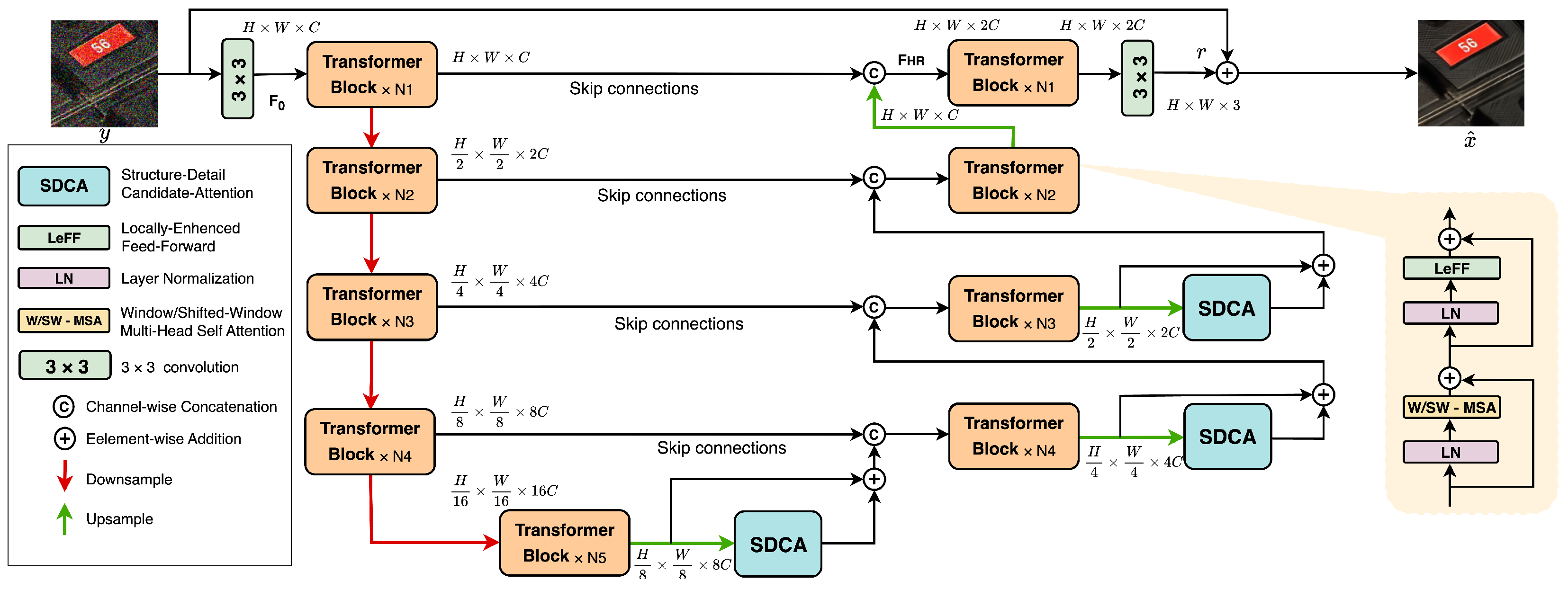
As shown in Figure 1, the proposed framework follows a U-shaped Transformer backbone, with SDCA inserted before encoder-decoder fusion at three decoder stages. Given a noisy input image $y\in {\mathbb{R}}^{B\times C_{\mathrm{in}}\times H\times W}$, where B denotes the batch size, $C_{\mathrm{in}}\in \{1,3\}$ is the number of input channels, and $H\times W$ denotes the spatial resolution, a $3\times 3$ convolution is first used to extract shallow features

$$F_0={\mathrm{conv}}_{3\times 3}\left(y\right).$$

(1)

The feature $F_0$ is then processed by a symmetric encoder-decoder backbone. The encoder progressively extracts hierarchical representations through downsampling, while the decoder restores spatial resolution through upsampling and skip fusion. Each stage consists of several Transformer blocks, where window-based self-attention, shifted-window self-attention, and a Locally Enhanced Feed-forward Network (LeFF) are used to model local and cross-window dependencies.

Unlike conventional U-shaped denoising models, SDCA is inserted into three intermediate-to-low-resolution decoder stages, excluding the highest-resolution stage, to balance restoration performance and computational cost. Let the decoder feature at the l-th insertion position be denoted as $U_l\in {\mathbb{R}}^{B\times C_l\times H_l\times W_l}$, where $l\in \{1,2,3\}$ corresponds to the decoder stages with spatial resolutions $H/8\times W/8$, $H/4\times W/4$, and $H/2\times W/2$. Before skip fusion, SDCA is inserted into the decoder branch and applied in a residual-injection manner

$${\tilde{U}}_l=U_l+\mathrm{SDCA}\left(U_l\right),$$

(2)

where $\mathrm{SDCA}(·)$ uses the decoder feature as the self-guidance signal to generate a calibration term with the same shape as $U_l$, and ${\tilde{U}}_l$ denotes the decoder feature after calibration. Subsequently, ${\tilde{U}}_l$ is concatenated with the corresponding encoder feature along the channel dimension and further refined by Transformer blocks. At the highest-resolution stage, a $3\times 3$ convolution maps the refined decoder feature $F_{HR}$ back to the image space to predict the residual image

$$r={\mathrm{conv}}_{3\times 3}\left(F_{HR}\right).$$

(3)

The final denoised output is obtained by global residual learning

$$\widehat{x}=y+r.$$

(4)

3.3. Structure–Detail Candidate Attention (SDCA)

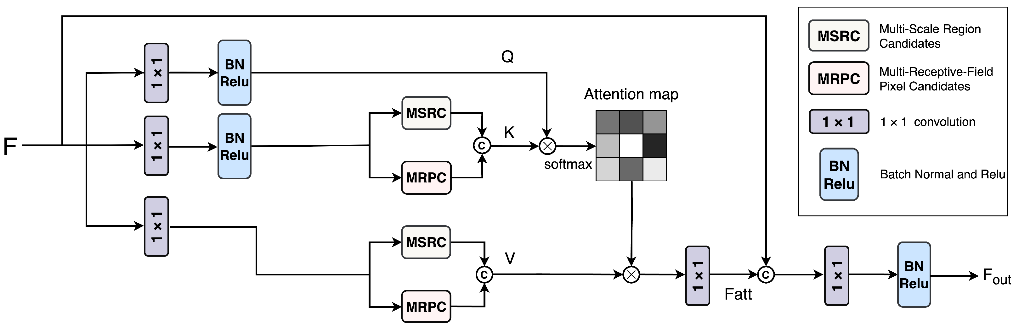
The proposed SDCA calibrates decoder features by retrieving complementary cues from a structure-detail candidate pool. As illustrated in Figure 2, given an input decoder feature $F\in {\mathbb{R}}^{B\times C\times H\times W}$, SDCA first projects it into query, key, and value feature maps using $1\times 1$ convolutions. To reduce computational cost, a channel reduction ratio $\rho$ is introduced, and the attention dimension is set to $d=C/\rho$ with $\rho =2$ in our implementation

$$\left\{\begin{array}{c}{Q}_0={\varphi }_q\left(F\right),\hfill \\ K_0={\varphi }_k\left(F\right),\hfill \\ V_0={\varphi }_v\left(F\right),\hfill \end{array}\right.$$

(5)

where $Q_0,K_0,V_0\in {\mathbb{R}}^{B\times d\times H\times W}$. Let $\mathrm{Tok}(·)$ flatten a feature map from ${\mathbb{R}}^{B\times d\times H\times W}$ to ${\mathbb{R}}^{B\times N\times d}$, where $N=H·W$. The pixel-wise query tokens are obtained as

$$Q=\mathrm{Tok}\left(Q_0\right).$$

(6)

For the key and value branches, MSRC generates region-level candidates, while MRPC generates pixel-level candidates

$$\begin{array}{cccc}\hfill K_r& =T_{\mathrm{MSRC}}^K\left(K_0\right),\hfill & \hfill K_p& =T_{\mathrm{MRPC}}^K\left(K_0\right),\hfill \\ \hfill V_r& =T_{\mathrm{MSRC}}^V\left(V_0\right),\hfill & \hfill V_p& =T_{\mathrm{MRPC}}^V\left(V_0\right),\hfill \end{array}$$

(7)

where $K_r,V_r\in {\mathbb{R}}^{B\times L_r\times d}$ and $K_p,V_p\in {\mathbb{R}}^{B\times L_p\times d}$. Since MRPC preserves the spatial resolution, $L_p=N$ generally holds. The region-level and pixel-level candidates are concatenated to form the K/V candidate pool

$$\left\{\begin{array}{c}K=[K_r;K_p],\hfill \\ V=[V_r;V_p],\hfill \end{array}\right.$$

(8)

where $K,V\in {\mathbb{R}}^{B\times L\times d}$ and $L=L_r+L_p$. Since SDCA is applied only at intermediate-to-low-resolution decoder stages, the size of the candidate pool remains computationally manageable.

Scaled dot-product attention is then performed between the pixel-wise queries and the candidate pool

$$Y=\mathrm{Softmax}\left({\displaystyle \frac{Q{K}^{\top }}{\sqrt{d}}}\right)V,$$

(9)

where $Y\in {\mathbb{R}}^{B\times N\times d}$ denotes the retrieved and aggregated token sequence. After inverse tokenization, a $1\times 1$ output projection maps the attention feature back to the original channel dimension

$$F_{\mathrm{att}}=W_o\left(\mathrm{UnTok}\left(Y\right)\right).$$

(10)

Finally, SDCA generates a residual calibration term through channel concatenation and learnable fusion

$$\Delta F=\mathsf{\gamma }\left({\mathrm{Cat}}_c(F_{\mathrm{att}},F)\right),$$

(11)

where ${\mathrm{Cat}}_c(·)$ denotes channel-wise concatenation, and $\mathsf{\gamma }(·)$ is a learnable fusion mapping composed of a $1\times 1$ convolution, Batch Normalization, and ReLU. The residual calibration term $\Delta F$ corresponds to the output of $\mathrm{SDCA}\left(F\right)$ in Equation (2).

3.4. Multi-Scale Region Candidates (MSRC)

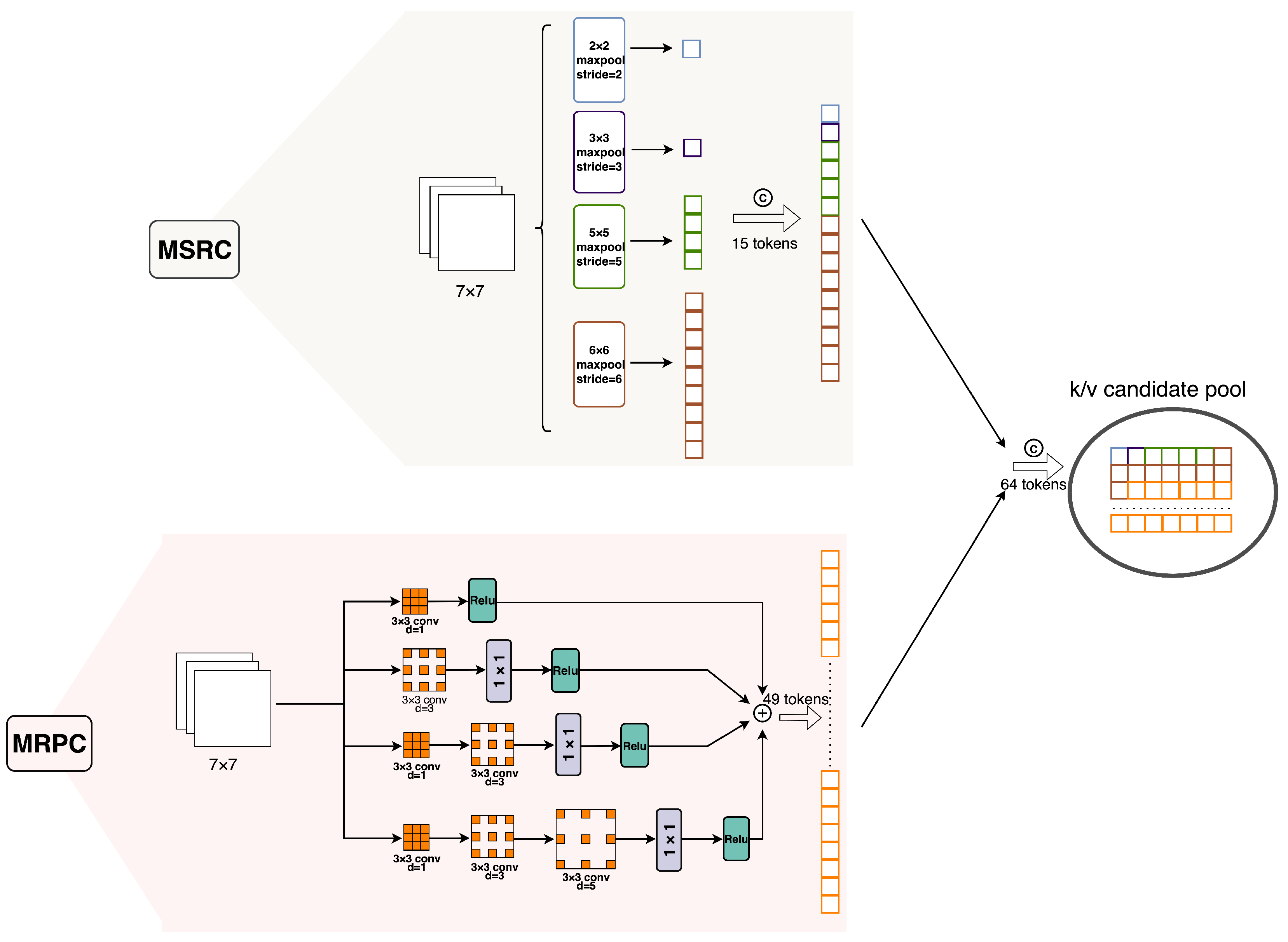
As illustrated in Figure 3, MSRC constructs region-level candidates by summarizing the input feature at multiple spatial granularities. Given an input feature $X\in {\mathbb{R}}^{B\times d\times H\times W}$, where $X=K_0$ in the key branch and $X=V_0$ in the value branch, a scale set $S=\{2,3,5,6\}$ is adopted. For each $s\in S$, a non-overlapping max pooling operator $P_s(·)$ with kernel size $s\times s$ and stride s is applied

$$X^{\left(s\right)}=P_s\left(X\right),$$

(12)

where $X^{\left(s\right)}\in {\mathbb{R}}^{B\times d\times H_s\times W_s}$, and 

$$H_s=⌊{\displaystyle \frac{H}{s}}⌋,W_s=⌊{\displaystyle \frac{W}{s}}⌋.$$

(13)

Only complete pooling regions are used, which avoids padding-induced boundary artifacts. Since MSRC is applied at intermediate-to-low-resolution decoder stages, the effect of boundary truncation is limited.

The multi-scale region features are flattened and concatenated along the token dimension

$$M_r={\mathrm{Concat}}_{\mathrm{tok}}\left({\left\{\mathrm{Tok}\left(X^{\left(s\right)}\right)\right\}}_{s\in S}\right),$$

(14)

where $M_r\in {\mathbb{R}}^{B\times L_r\times d}$ and

$$L_r=\sum _{s\in S}{H}_s{W}_s=\sum _{s\in S}⌊{\displaystyle \frac{H}{s}}⌋⌊{\displaystyle \frac{W}{s}}⌋.$$

(15)

3.5. Multi-Receptive-Field Pixel Candidates (MRPC)

As depicted in Figure 3, MRPC constructs pixel-level candidates by introducing multi-receptive-field context while preserving the spatial resolution. Given $X\in {\mathbb{R}}^{B\times d\times H\times W}$, let $C_{\delta }(·)$ denote a $3\times 3$ dilated convolution with dilation rate $\delta$, $G(·)$ denote a $1\times 1$ channel-alignment convolution, and $\mathsf{\sigma }(·)$ denote the ReLU activation. MRPC uses four parallel branches with different effective receptive fields

$$\left\{\begin{array}{c}{F}^{\left(1\right)}=\mathsf{\sigma }\left(C_1\left(X\right)\right),\hfill \\ F^{\left(2\right)}=\mathsf{\sigma }\left(G\left(C_3\left(X\right)\right)\right),\hfill \\ F^{\left(3\right)}=\mathsf{\sigma }\left(G\left(C_3\left(C_1\left(X\right)\right)\right)\right),\hfill \\ F^{\left(4\right)}=\mathsf{\sigma }\left(G\left(C_5\left(C_3\left(C_1\left(X\right)\right)\right)\right)\right).\hfill \end{array}\right.$$

(16)

Since all branches preserve the resolution, their outputs are fused by element-wise summation

$$U\left(X\right)=\sum _{i=1}^4{F}^{\left(i\right)}.$$

(17)

The fused feature is then flattened into pixel-level candidate tokens

$$M_p=\mathrm{Tok}\left(U\left(X\right)\right).$$

(18)

3.6. Loss Function

The proposed method is trained using the Charbonnier loss, which is defined as follows:

$${\mathcal{L}}_{\mathrm{Charbonnier}}(\widehat{x},x)={\displaystyle \frac{1}{N}}\sum _{i=1}^N\sqrt{{({\widehat{x}}_i-x_i)}^2+{\epsilon }^2},$$

(19)

where ${\widehat{x}}_i$ and $x_i$ denote the network prediction and the corresponding ground-truth value, respectively. $\epsilon$ is a very small constant and is set to ${10}^{-3}$ in this paper to avoid numerical instability when the residual approaches zero. In image denoising, commonly used loss functions include the $L_1$ loss and the $L_2$ loss. The $L_1$ loss computes the sum of absolute residuals and is relatively robust to outliers. In contrast, the $L_2$ loss computes the sum of squared residuals, which is smoother and easier to optimize but more sensitive to large deviations. The Charbonnier loss inherits the robustness of the $L_1$ loss to outliers while also exhibiting continuity and differentiability similar to those of the $L_2$ loss. Therefore, it is more stable and effective for low-level vision tasks such as image denoising.

4. Experimental Results and Analysis

4.1. Implementation Details

The proposed network was implemented in PyTorch 2.0.0 and trained on an NVIDIA GeForce RTX 4090 GPU. Unless otherwise specified, the proposed model was trained under the following settings. During training, paired noisy-clean patches of size $256\times 256$ were randomly cropped from the corresponding image pairs, where the same cropping position was used for the noisy input and clean reference to maintain pixel-level alignment. Random geometric augmentation was adopted, including rotations, flipping operations, and their combinations. In addition, MixUp augmentation was applied after the first five epochs, with the mixing coefficient sampled from a Beta distribution with $\alpha =\beta =1.2$. The batch size was set to 16, and the model was trained for 105 epochs. The AdamW optimizer was employed with an initial learning rate of $2\times {10}^{-4}$, ${\beta }_1=0.9$, ${\beta }_2=0.999$, $ϵ={10}^{-8}$, and a weight decay of 0.02. A StepLR scheduler was adopted to reduce the learning rate by a factor of 0.5 every 50 epochs. The Charbonnier loss was used as the optimization objective, and mixed-precision training was enabled using automatic mixed precision and gradient scaling. The random seed was set to 1234 in the training script to improve reproducibility.

Two standard full-reference metrics are adopted to quantitatively evaluate image denoising performance.

Peak Signal-to-Noise Ratio (PSNR): A fidelity metric based on Mean Squared Error (MSE), where a higher value denotes better noise suppression and higher consistency with the ground-truth. The formula is

$$\mathrm{PSNR}=10·{log}_{10}\left({\displaystyle \frac{{\mathrm{MAX}}_I^2}{\mathrm{MSE}}}\right),\mathrm{MSE}={\displaystyle \frac{1}{HWC}}\sum _{i=1}^H\sum _{j=1}^W\sum _{c=1}^C{(I_{i,j,c}-{\widehat{I}}_{i,j,c})}^2$$

(20)

where H, W, C are the height, width, and channel number of the image; I and $\widehat{I}$ denote the ground-truth and denoised image; ${\mathrm{MAX}}_I=1$ for normalized images.

Structural Similarity Index Measure (SSIM): Evaluates structural preservation from luminance, contrast, and structure. Its value ranges from 0 to 1, and a value closer to 1 indicates better detail recovery. The standard formula is

$$\mathrm{SSIM}(x,y)={\displaystyle \frac{(2{\mu }_x{\mu }_y+C_1)(2{\sigma }_{xy}+C_2)}{({\mu }_x^2+{\mu }_y^2+C_1)({\sigma }_x^2+{\sigma }_y^2+C_2)}}$$

(21)

where ${\mu }_x/{\mu }_y$ are local means, ${\sigma }_x/{\sigma }_y$ are local variances, ${\sigma }_{xy}$ is the local covariance, and $C_1,C_2$ are stability constants.

For color and real-world denoising experiments, PSNR was computed on normalized RGB images with the maximum pixel value set to 1, and SSIM was calculated using the pytorch-msssim implementation with data_range = 1.0. For grayscale denoising, the metrics were computed on the corresponding grayscale images. For benchmarks without publicly available ground-truth images, the official evaluation protocol was followed. Validation was performed after each training epoch, and the average metrics over the validation set were reported. The numbers of Transformer blocks from $N_1$ to $N_5$ were 1, 2, 8, 8, and 2, respectively, as detailed in

Table 1. Experimental settings of the proposed model.

Parameter	Value
Framework	PyTorch
GPU	NVIDIA GeForce RTX 4090
Input patch size	$256\times 256$
Batch size	16
Training epochs	105
Optimizer	AdamW
Initial learning rate	$2\times {10}^{-4}$
${\beta }_1$, ${\beta }_2$, $ϵ$	0.9, 0.999, $1\times {10}^{-8}$
Weight decay	0.02
Loss function	Charbonnier loss
MixUp setting	Applied after 5 epochs, $\alpha =\beta =1.2$
Evaluation data range	$[0,1]$
Numbers of Transformer blocks $N_1$–$N_5$	1, 2, 8, 8, 2

.

4.2. Datasets

Synthetic Gaussian denoising: In the synthetic Gaussian denoising experiments, the proposed network was trained on the DIV2K-Flickr2K-WED-BSD400 (DFWB) synthetic training set, which consists of the DIVerse 2K resolution image dataset (DIV2K) [42], Flickr 2K dataset (Flickr2K) [43], Waterloo Exploration Database (WED) [44], and Berkeley Segmentation Dataset (BSD400) [45]. During training, $256\times 256$ patches were randomly cropped from clean images in DFWB, and additive white Gaussian noise (AWGN) was injected according to the specified noise levels. During the testing phase, the proposed method was evaluated on several widely adopted benchmark datasets. Specifically, the grayscale benchmarks include Set12 [14], BSD68 [45], and Urban100 [46], while the color benchmarks include CBSD68 [45], Kodak24 [47], McMaster [48], and Urban100 [46]. These datasets contain a wide variety of image content, including natural scenes, rich texture patterns, and complicated urban structures, which makes them suitable for comprehensively assessing the generalization capability of the proposed model across different image structures and texture characteristics.

Real-world denoising: For real-world image denoising, the Smartphone Image Denoising Dataset (SIDD) [49] was used for training. This dataset contains 320 pairs of real noisy images and their corresponding clean reference images captured by real imaging devices. During training, $256\times 256$ patches were randomly cropped from the paired images. For performance evaluation, the proposed method was tested on the SIDD validation set and the Darmstadt Noise Dataset (DND) [50]. The SIDD validation set includes 40 images, and its official evaluation protocol is commonly conducted on 1280 patches extracted from these images. The DND dataset contains 50 image pairs, while the corresponding clean reference images are not publicly released. Therefore, the denoised outputs were uploaded to the official DND evaluation server, from which the Peak Signal-to-Noise Ratio (PSNR) [51] and Structural Similarity Index Measure (SSIM) [52] were obtained.

4.3. Comparative Experiments

We systematically evaluated the proposed UT-DPFC under both synthetic Gaussian and real-world noise settings. For synthetic Gaussian denoising, to cover representative methods ranging from traditional prior-based approaches to deep learning models, the classical prior-based method BM3D [12] was included for comparison. Typical CNN-based methods, including DnCNN [14], FFDNet [15], NLRN [34], MWCNN [53], RNAN [35], and DRUNet [18], were selected as baseline models. In addition, Transformer-based restoration models, such as SwinIR [22], SCUNet [54], and Restormer [25], were included, together with recent advanced networks, including KBNet [55], CGNet [56], EAMamba [29], and DSCA-former [36]. To further strengthen the comparison with recent U-shaped Transformer-based restoration networks, FUT [30] and RUST [31] were also incorporated into the quantitative evaluation.

For real-world denoising, in addition to DnCNN [14], representative real-noise modeling methods, including CBDNet [16], RIDNet [57], and AINDNet [58], were also included for comparison, together with multi-stage image restoration methods such as CycleISP [59], MIRNet [60], and MPRNet [61]. The proposed method was further compared with Transformer-based models, including Uformer [23], Restormer [25], and Xformer [62], as well as recent methods such as MambaIR [63], DRANet [64], and AKDT [65]. These comparisons provided a more comprehensive validation of the effectiveness and generalization ability of the proposed method under both synthetic and real-world noise settings.

4.3.1. Synthetic Gaussian Denoising (Grayscale)

Under the synthetic additive white Gaussian noise (AWGN) grayscale denoising setting, UT-DPFC was evaluated on Set12, BSD68, and Urban100 at noise levels of $\sigma =15$, 25, and 50. As shown in

Table 2. Quantitative comparison results in terms of PSNR/SSIM for Gaussian grayscale image denoising on the Set12, BSD68, and Urban100 datasets. In each setting, the best result is shown in bold, and the second-best result is underlined. When multiple methods achieve the same rounded value, only one representative result is highlighted for readability.

Method	Set12			BSD68			Urban100
	$\sigma =\mathbf{15}$	$\sigma =\mathbf{25}$	$\sigma =\mathbf{50}$	$\sigma =\mathbf{15}$	$\sigma =\mathbf{25}$	$\sigma =\mathbf{50}$	$\sigma =\mathbf{15}$	$\sigma =\mathbf{25}$	$\sigma =\mathbf{50}$
BM3D [12]	32.37/0.896	29.97/0.851	26.72/0.766	31.08/0.872	28.57/0.802	25.60/0.687	32.35/0.922	29.70/0.878	25.95/0.779
DnCNN [14]	32.86/0.903	30.44/0.862	27.18/0.783	31.73/0.891	29.23/0.828	26.23/0.719	32.64/0.926	29.95/0.880	26.26/0.788
FFDNet [15]	32.75/0.903	30.43/0.864	27.32/0.791	31.63/0.890	29.19/0.830	26.29/0.726	32.40/0.927	29.90/0.898	26.50/0.805
NLRN [34]	33.16/0.907	30.80/0.869	27.64/0.798	31.88/0.893	29.41/0.833	26.47/0.730	33.45/0.935	30.94/0.902	27.49/0.828
MWCNN [53]	33.15/0.909	30.79/0.871	27.74/0.806	31.86/0.895	29.41/0.836	26.53/0.737	33.17/0.936	30.66/0.903	27.42/0.837
RNAN [35]	-	-	27.70/0.796	-	-	26.48/0.731	-	-	27.65/0.820
DRUNet [18]	33.25/0.910	30.94/0.873	27.90/0.810	31.91/0.894	29.48/0.836	26.59/0.737	33.44/0.937	31.11/0.908	27.96/0.848
SwinIR [22]	33.36/0.911	31.01/0.874	27.91/0.810	31.97/0.895	29.50/0.837	26.58/0.737	33.70/0.939	31.30/0.909	27.98/0.848
Restormer [25]	33.42/0.912	31.08/0.875	28.00/0.812	31.96/0.896	29.52/0.838	26.62/0.741	33.79/0.939	31.46/0.911	28.29/0.856
KBNet [55]	33.40/0.912	31.08/0.876	28.04/0.814	31.98/0.897	29.54/0.839	26.65/0.741	33.77/0.939	31.45/0.910	28.33/0.857
DSCA-former [36]	33.26/0.910	30.94/0.872	27.91/0.809	31.97/0.896	29.52/0.838	26.59/0.738	33.80/0.940	31.48/0.912	28.32/0.857
RUST [31]	32.85/0.903	30.53/0.864	27.45/0.794	-	-	-	-	-	-
Ours	33.38/0.912	31.10/0.876	28.05/0.814	32.01/0.897	29.52/0.838	26.69/0.742	33.79/0.940	31.48/0.912	28.36/0.858

, the proposed method achieves competitive and consistent PSNR/SSIM performance across different datasets and noise levels. In terms of PSNR, UT-DPFC obtains the best results in 6 out of 9 settings, including Set12 at $\sigma =25$ and $\sigma =50$, BSD68 at $\sigma =15$ and $\sigma =50$, and Urban100 at $\sigma =25$ and $\sigma =50$. In particular, under the high-noise setting of $\sigma =50$, UT-DPFC achieves the best PSNR on all three datasets, reaching 28.05 dB on Set12, 26.69 dB on BSD68, and 28.36 dB on Urban100. This indicates that the proposed method has strong robustness under severe Gaussian noise degradation. The performance gain under heavy noise mainly comes from the SDCA calibration, which cleans decoder features before fusion and reduces noise contamination during encoder-decoder fusion.

In terms of SSIM, UT-DPFC also shows stable structural restoration capability. It achieves the best or tied-best SSIM in most settings, especially on Urban100, where it obtains the best SSIM values of 0.940, 0.912, and 0.858 at $\sigma =15$, 25, and 50, respectively. Since Urban100 contains abundant repetitive structures and complex textures, the consistent advantage of this dataset suggests that the proposed decoder-side pre-fusion calibration is beneficial for preserving structural information and texture details. Overall, the grayscale denoising results demonstrate that UT-DPFC provides stable restoration quality across different noise levels, with more evident advantages under high-noise and complex-texture conditions.

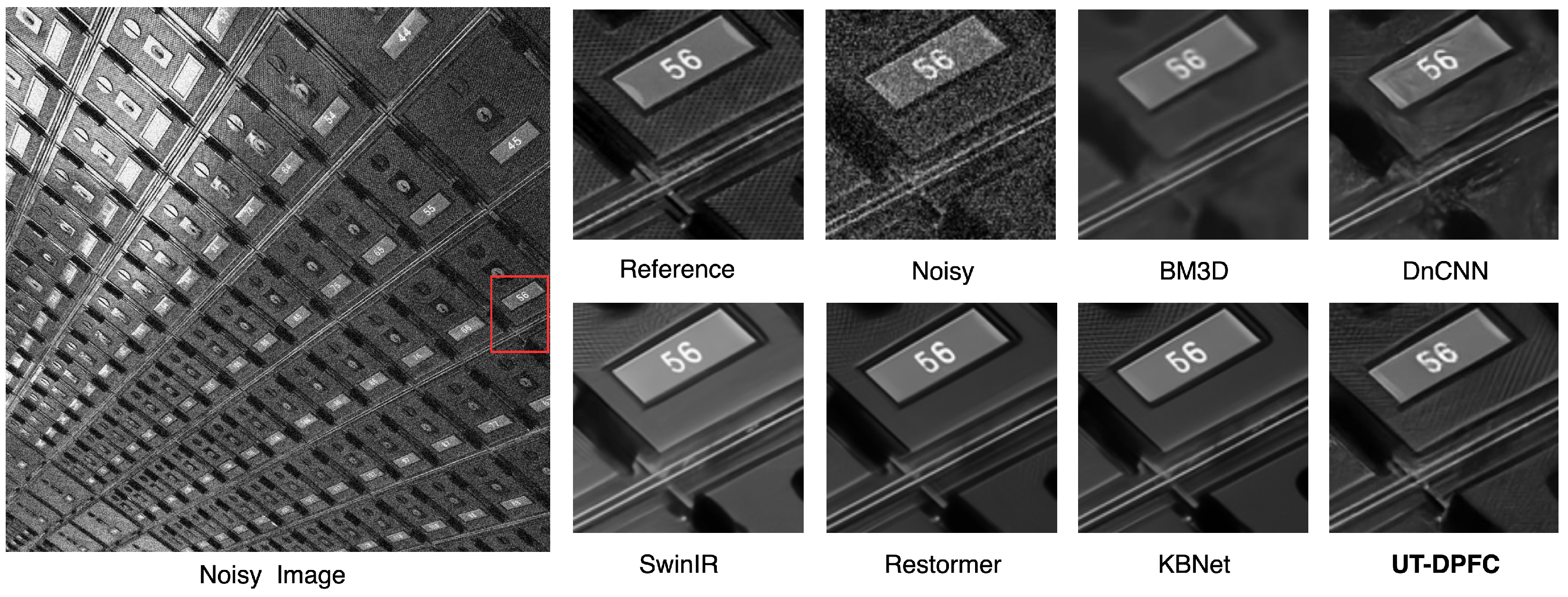
The qualitative comparisons in Figure 4 and Figure 5 further support the quantitative results. As shown in Figure 4, for the Urban100 image with dense repetitive stripe structures under the high-noise setting of $\sigma =50$, BM3D and DnCNN tend to over-smooth the restored image, resulting in weakened fine textures and blurred structural details. Although SwinIR, Restormer, and KBNet suppress noise more effectively, they still show limited recovery of dense high-frequency stripe patterns. In contrast, UT-DPFC better preserves the continuity and clarity of the repetitive structures while maintaining effective noise suppression.

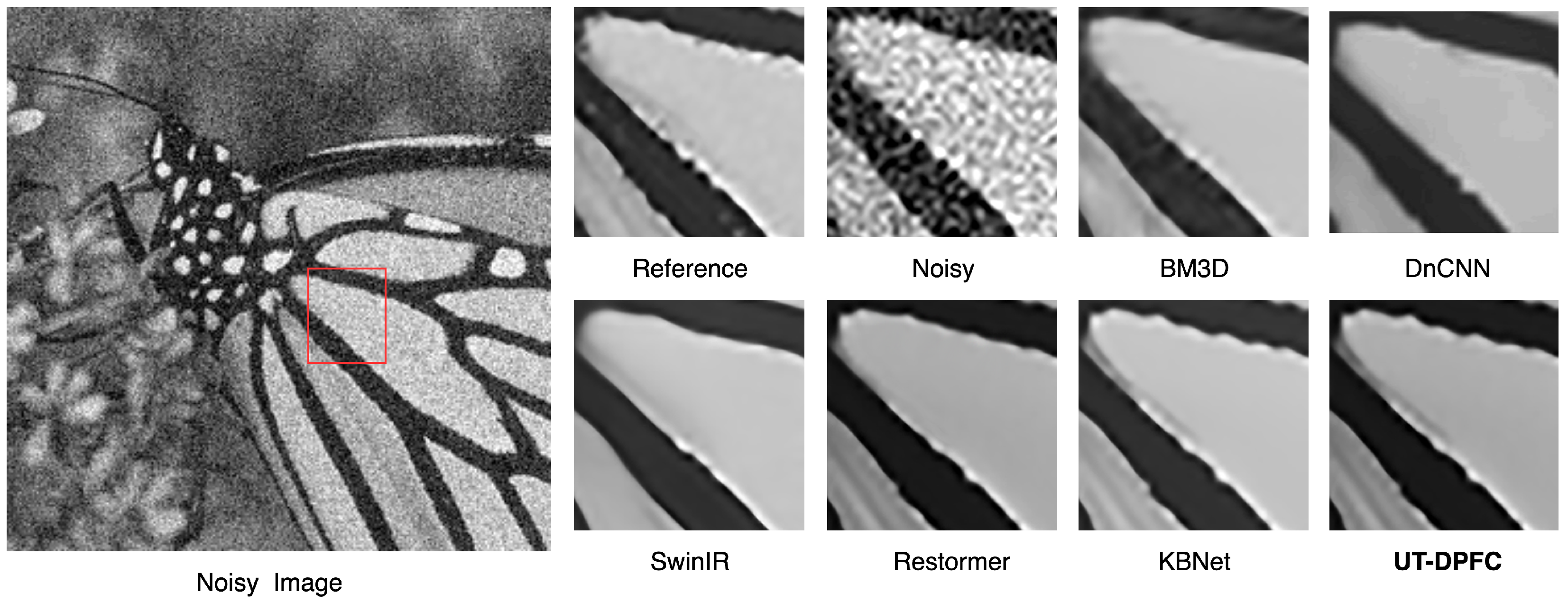
Figure 5 further presents a visual comparison on the Set12 dataset with $\sigma =25$. In the butterfly wing region, BM3D and DnCNN introduce noticeable texture distortion and edge blurring after denoising. SwinIR, Restormer, and KBNet recover smoother results, but some fine boundaries and local structural transitions are still weakened. By comparison, UT-DPFC produces sharper wing boundaries and more stable local texture restoration, showing better consistency with the reference image. These visual results indicate that the proposed decoder-side pre-fusion calibration is beneficial for preserving structural details and fine textures under both moderate and high Gaussian noise levels.

4.3.2. Synthetic Gaussian Denoising (Color)

Under the synthetic additive white Gaussian noise (AWGN) image denoising setting, UT-DPFC is evaluated on four benchmark datasets: CBSD68, Kodak24, McMaster, and Urban100, across three noise levels of $\sigma =15$, 25, and 50, resulting in a total of 12 test settings. As shown in

Table 3. Quantitative comparison results in terms of PSNR/SSIM for Gaussian color image denoising on the CBSD68, Kodak24, McMaster, and Urban100 datasets. In each setting, the best result is shown in bold, and the second-best result is underlined. When multiple methods achieve the same rounded value, only one representative result is highlighted for readability.

Method	CBSD68			Kodak24			McMaster			Urban100
	$\sigma =\mathbf{15}$	$\sigma =\mathbf{25}$	$\sigma =\mathbf{50}$	$\sigma =\mathbf{15}$	$\sigma =\mathbf{25}$	$\sigma =\mathbf{50}$	$\sigma =\mathbf{15}$	$\sigma =\mathbf{25}$	$\sigma =\mathbf{50}$	$\sigma =\mathbf{15}$	$\sigma =\mathbf{25}$	$\sigma =\mathbf{50}$
BM3D [12]	33.52/0.922	30.71/0.868	27.38/0.763	34.28/0.916	32.15/0.868	28.46/0.775	34.06/0.904	31.66/0.874	28.51/0.794	33.93/0.941	31.36/0.909	27.93/0.840
DnCNN [14]	33.90/0.929	31.24/0.883	27.95/0.789	34.60/0.921	32.14/0.878	28.95/0.792	33.45/0.904	31.52/0.869	28.62/0.799	32.98/0.931	30.81/0.901	27.59/0.833
FFDNet [15]	33.87/0.929	31.21/0.882	27.96/0.789	34.63/0.922	32.13/0.879	28.98/0.795	34.66/0.922	32.35/0.886	29.18/0.815	33.83/0.942	31.40/0.912	28.05/0.848
RNAN [35]	-	-	28.27/0.802	-	-	29.58/0.812	-	-	29.72/0.833	-	-	29.08/0.870
DRUNet [18]	34.30/0.934	31.69/0.892	28.51/0.810	35.31/0.929	32.89/0.892	29.86/0.821	35.40/0.932	33.14/0.903	30.08/0.846	34.81/0.951	32.60/0.928	29.61/0.883
SwinIR [22]	34.42/0.936	31.78/0.894	28.56/0.812	35.34/0.930	32.89/0.893	29.79/0.822	35.61/0.935	33.20/0.906	30.22/0.849	35.13/0.952	32.90/0.931	29.82/0.886
SCUNet [54]	34.40/0.935	31.79/0.893	28.61/0.813	35.34/0.930	32.92/0.893	29.87/0.821	35.60/0.935	33.34/0.906	30.29/0.851	35.13/0.952	32.96/0.931	30.02/0.879
Restormer [25]	34.40/0.935	31.79/0.894	28.60/0.813	35.47/0.930	33.04/0.893	30.01/0.823	35.61/0.934	33.34/0.906	30.30/0.852	35.13/0.952	32.96/0.931	30.02/0.890
CGNet [56]	34.41/0.934	31.79/0.894	28.60/0.813	35.52/0.931	33.07/0.894	30.06/0.824	35.58/0.934	33.28/0.905	30.22/0.850	35.18/0.953	32.98/0.932	30.07/0.891
KBNet [55]	34.41/0.936	31.80/0.894	28.62/0.814	35.46/0.930	33.05/0.894	30.04/0.823	35.56/0.934	33.31/0.906	30.27/0.851	35.15/0.952	32.96/0.931	30.04/0.891
EAMamba [29]	34.43/0.936	31.81/0.895	28.62/0.814	35.36/0.930	32.95/0.893	29.91/0.822	35.59/0.935	33.34/0.905	30.31/0.853	-	-	-
DSCA-former [36]	34.43/0.936	31.80/0.894	28.53/0.812	35.49/0.931	32.99/0.893	29.76/0.820	35.65/0.936	33.32/0.906	30.25/0.851	-	-	-
RUST [31]	34.15/0.932	31.48/0.888	28.30/0.802	34.86/0.924	32.39/0.887	29.24/0.805	35.07/0.927	32.66/0.894	29.47/0.829	-	-	-
FUT [30]	34.08/0.932	31.44/0.888	28.28/0.802	34.89/0.925	32.46/0.885	29.39/0.811	35.16/0.929	32.84/0.898	29.75/0.837	-	-	-
Ours	34.43/0.936	31.80/0.895	28.63/0.815	35.50/0.931	33.09/0.895	30.08/0.824	35.61/0.935	33.35/0.907	30.33/0.853	35.16/0.953	33.01/0.933	30.10/0.893

, the proposed method achieves stable PSNR/SSIM performance across all datasets and noise levels. In terms of PSNR, UT-DPFC achieves the optimal results in 8 out of 12 settings. Notably, under the high-noise setting of $\sigma =50$, UT-DPFC obtains the best PSNR results on all four datasets: 28.63 dB on CBSD68, 30.08 dB on Kodak24, 30.33 dB on McMaster, and 30.10 dB on Urban100. The consistent performance improvement under heavy color noise is also attributed to the SDCA module, which calibrates decoder features to suppress noise interference and stabilize cross-scale feature fusion. This reflects the robustness of the method under severe Gaussian noise degradation scenarios. In terms of SSIM, UT-DPFC demonstrates stable structural restoration capability and achieves the optimal results in most settings. Especially on the texture-rich Urban100 dataset, the method achieves leading SSIM values of 0.953, 0.933, and 0.893 at $\sigma =15$, 25, and 50, respectively. Since Urban100 contains abundant repetitive structures and complex textures, this consistent advantage indicates that the proposed decoder-side pre-fusion calibration strategy is beneficial for preserving structural information and fine-grained texture details.

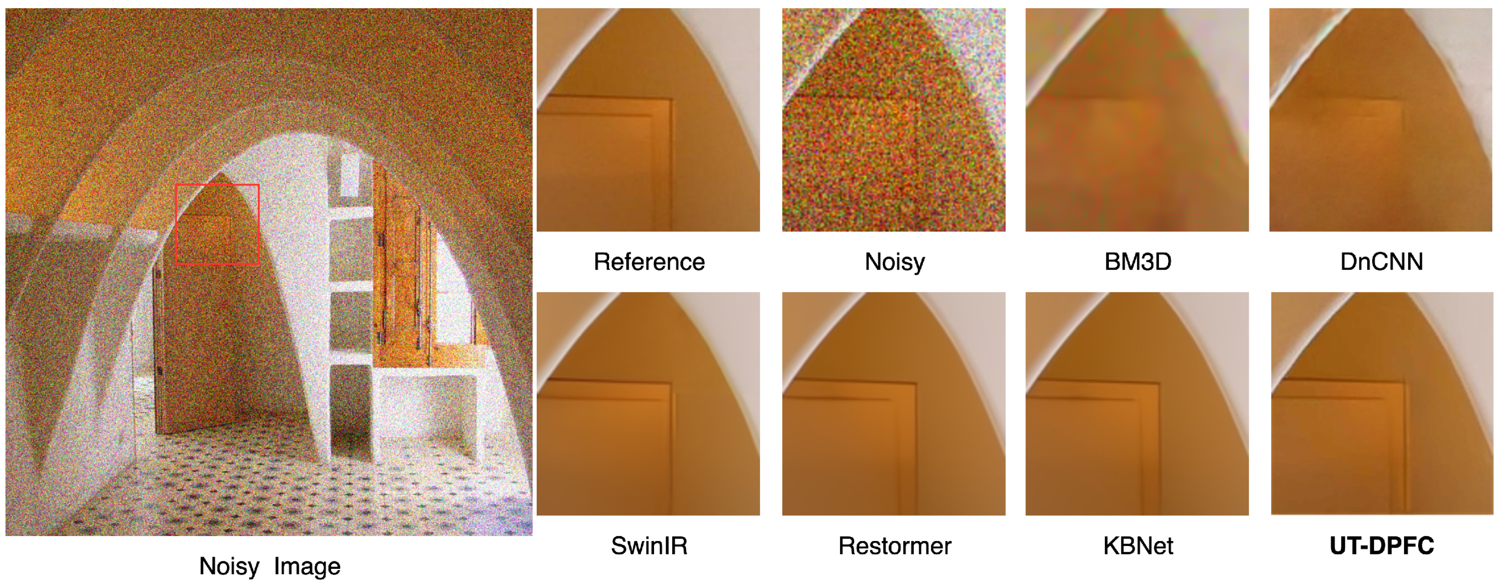
The qualitative comparisons in Figure 6 and Figure 7 further support the quantitative results. As shown in Figure 6, for the Urban100 image under the high-noise setting of $\sigma =50$, BM3D and DnCNN remove part of the noise but tend to over-smooth the restored image, leading to blurred curved edges and weakened thin door-frame structures. SwinIR, Restormer, and KBNet achieve stronger noise suppression, but some fine structures and local boundary transitions are still not fully recovered. In contrast, UT-DPFC more clearly restores the thin door-frame lines and adjacent edge contours while maintaining effective noise suppression, resulting in sharper structural boundaries and more natural visual transitions.

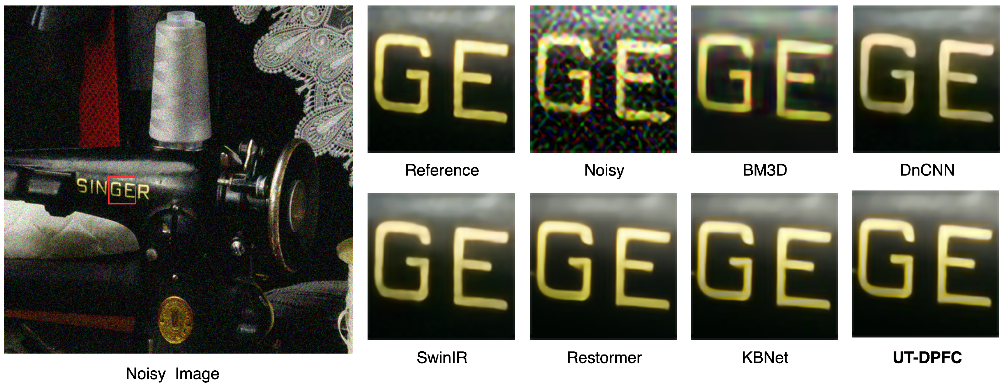
Figure 7 further presents a visual comparison on the McMaster dataset with $\sigma =25$. In the enlarged character region, BM3D and DnCNN produce over-smoothed results, where the character boundaries become blurred and local details are weakened. Although SwinIR, Restormer, and KBNet recover more visually pleasing results, slight boundary softness and detail loss can still be observed around the character strokes. By comparison, UT-DPFC preserves clearer character contours and more stable local contrast, showing better consistency with the reference image. These visual results demonstrate that the proposed decoder-side pre-fusion calibration helps preserve structural edges and fine color details under both moderate and high Gaussian noise levels.

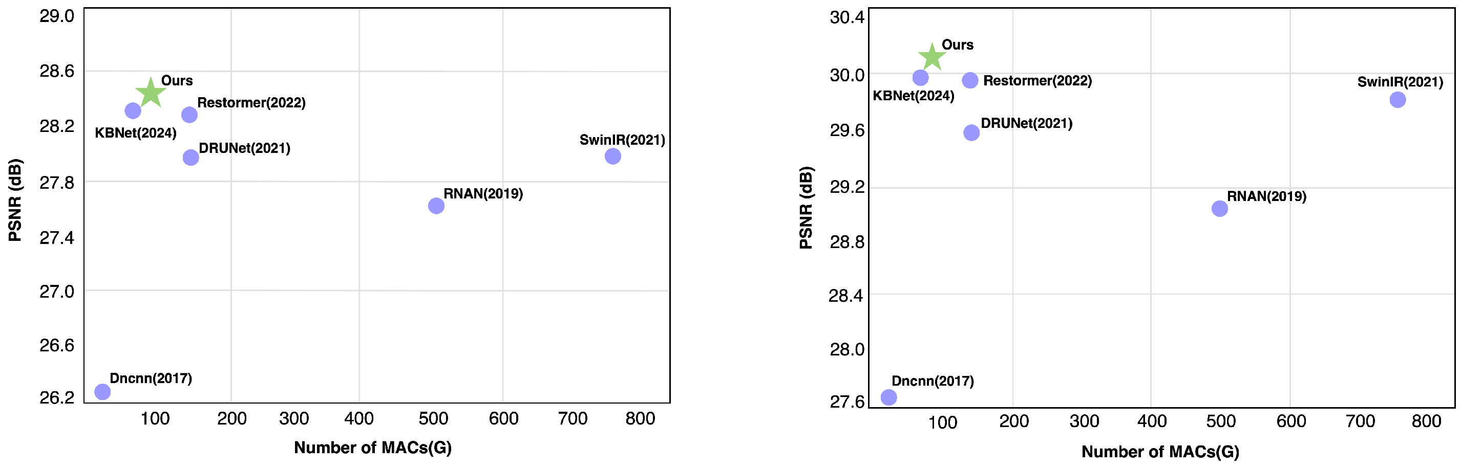
Figure 8 presents PSNR-MACs scatter plots for grayscale and color image denoising on Urban100, where MACs were measured with an input size of $256\times 256$.

4.3.3. Real-World Image Denoising

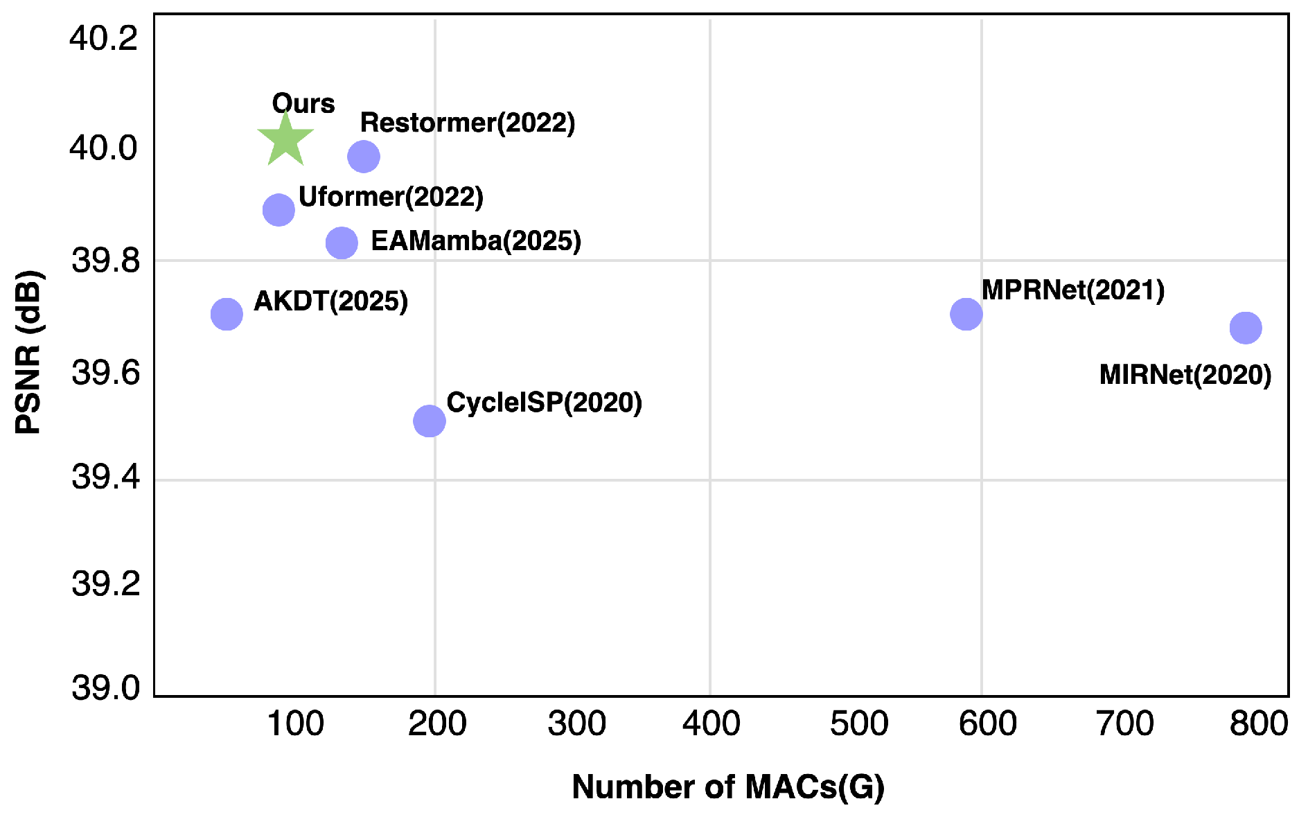
To verify the effectiveness and generalization ability of the proposed method under real-world noise, we report the average PSNR and SSIM results on the SIDD and DND benchmarks. As shown in

Table 4. Quantitative comparison results for real-world image denoising on the SIDD and DND datasets. The best result is shown in bold, and the second-best result is underlined.

Method	SIDD		DND
	PSNR	SSIM	PSNR	SSIM
DnCNN [14]	23.66	0.583	32.43	0.790
CBDNet [16]	30.78	0.801	38.06	0.942
RIDNet [57]	38.71	0.951	39.26	0.953
AINDNet [58]	39.08	0.954	39.37	0.951
CycleISP [59]	39.52	0.957	39.56	0.956
MIRNet [60]	39.72	0.959	39.88	0.956
MPRNet [61]	39.71	0.958	39.80	0.954
Uformer [23]	39.89	0.959	39.98	0.955
Restormer [25]	40.02	0.960	40.03	0.956
Xformer [62]	39.98	0.960	40.19	0.957
DRANet [64]	39.50	0.957	39.64	0.952
MambaIR [63]	39.89	0.960	40.04	0.956
AKDT [65]	39.70	0.961	–	–
EAMamba [29]	39.87	0.960	–	–
Ours	40.03	0.960	40.01	0.956

, UT-DPFC performs well compared with existing representative methods. Specifically, the method achieves a performance level comparable to that of mainstream existing approaches on the SIDD dataset, while also obtaining reasonably satisfactory results on the DND benchmark. To further illustrate the performance-complexity trade-off under real-world noise,

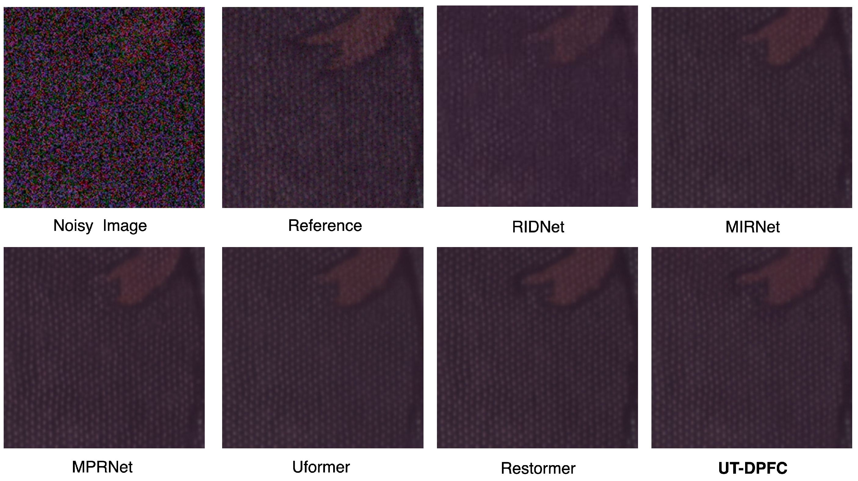
The qualitative comparisons shown in Figure 9 further supported the above observations. In texture-rich regions and around weak edges, RIDNet, MIRNet, MPRNet, and Uformer tended to exhibit texture discontinuities or slight over-smoothing. In contrast, UT-DPFC and Restormer were generally able to suppress noise while preserving more coherent texture structures and more stable edge contours.

Figure 10 presents a PSNR-MACs scatter plot on SIDD, where MACs were measured with an input size of $256\times 256$.

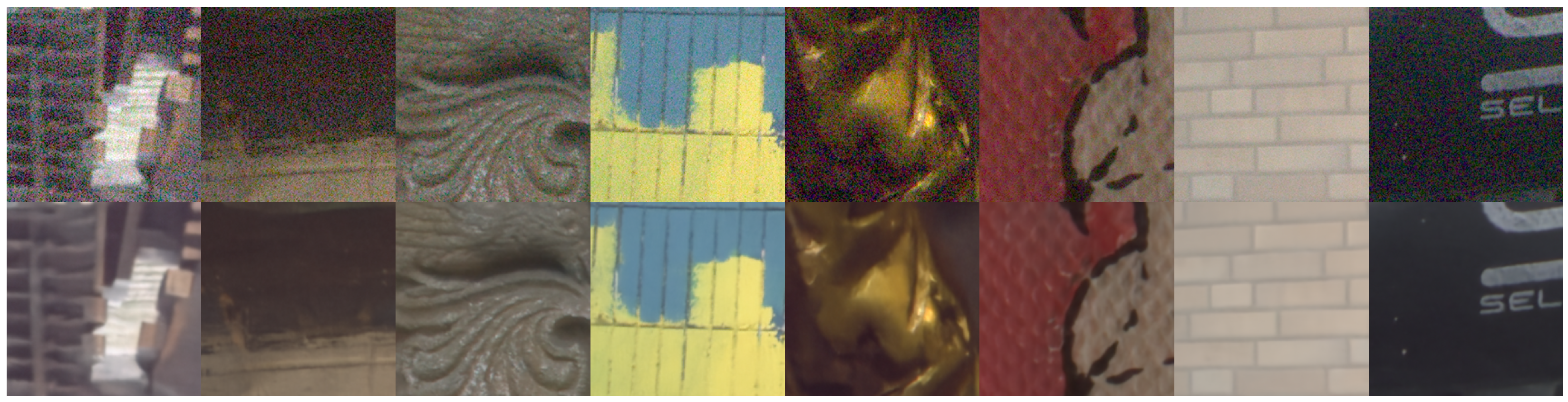
To further validate the real-world denoising capability of the proposed method, several denoised examples from the DND dataset were presented in Figure 11, showing that the proposed method could effectively remove real-world noise.

4.4. Region-Wise Error Analysis

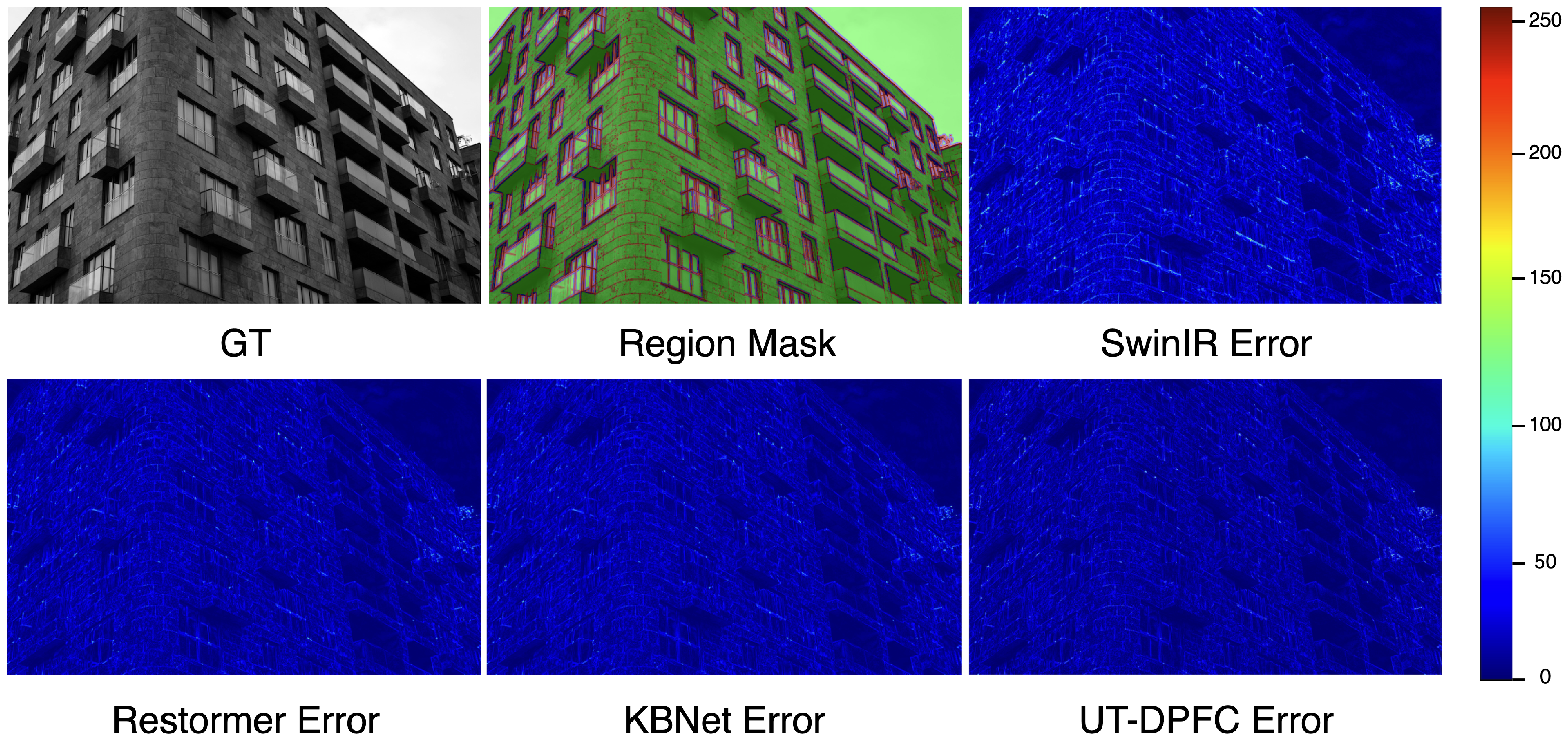
To further analyze the restoration behavior of different methods in high-noise and complex-texture scenarios beyond the overall PSNR/SSIM comparison, we conducted region-wise Root Mean Square Error(RMSE) statistics on Urban100 with $\sigma =50$. Specifically, the images were divided into flat regions, edge regions, and texture-rich regions. Urban100 is one of the important benchmarks for synthetic Gaussian denoising, and $\sigma =50$ corresponds to a high-noise setting, which is more suitable for observing the restoration differences of different methods in complex texture and structural regions. As shown in

Table 5. Region-wise RMSE comparison on Urban100 with $\sigma =50$.

Method	Smooth RMSE	Edge RMSE	Texture-Rich RMSE
SwinIR [22]	0.0468	0.1392	0.1104
Restormer [25]	0.0425	0.1283	0.1015
KBNet [55]	0.0418	0.1227	0.0989
Ours	0.0402	0.1179	0.0972

, UT-DPFC achieves the lowest RMSE in all three types of regions, with RMSE values of 0.0402, 0.1179, and 0.0972 in flat, edge, and texture-rich regions, respectively. Compared with SwinIR, UT-DPFC reduces the RMSE by 0.0066, 0.0213, and 0.0132 in the three regions, respectively. Compared with Restormer, the corresponding reductions are 0.0023, 0.0104, and 0.0043, while compared with KBNet, the RMSE is further reduced by 0.0016, 0.0048, and 0.0017, respectively. The lower RMSE under heavy noise indicates that the pre-fusion calibration effectively suppresses noise disturbance in edge and texture regions, leading to more robust restoration. These results indicate that the proposed decoder-side pre-fusion calibration not only benefits detail restoration in texture-rich regions, but also improves structural reconstruction in edge regions, while maintaining stable denoising capability in flat regions. The representative examples in Figure 12 further show that UT-DPFC produces weaker error responses around dense facade textures and structural boundaries, with more concentrated error distributions, especially in texture-rich and edge regions. This observation is consistent with the above analysis of the restoration advantages of the proposed method under high-noise and complex-texture conditions.

4.5. Model Runtime Analysis

In this subsection, model complexity was further evaluated by comparing the runtime of different methods. The compared models included BM3D [12], MCWNNM [66], IRCNN [67], DnCNN-B [14], FFDNet [15], ADNet [68], SADNet [69], CycleISP [59], AINDNet [58], AirNet [70], and DRANet [64]. Among them, BM3D and MCWNNM were implemented in MATLAB (R2020a), while the remaining denoising models were implemented in the PyTorch environment. The runtime results were reported in Table 6. Specifically, two synthetic noisy images with different channel numbers and spatial resolutions of $256\times 256$ and $512\times 512$, respectively, were randomly selected at a noise level of $\sigma =25$ to evaluate inference speed. The runtime values in Table 6 were obtained by averaging 20 repeated runs for each denoising model. It should be noted that the memory transfer time between the CPU and GPU was not included in the measurement. As shown in Table 6, the proposed method (Ours) exhibited clear efficiency advantages in GPU inference at both input resolutions. For $256\times 256$ inputs, it ran faster than DRANet, AINDNet and AirNet. For $512\times 512$ inputs, its runtime remained significantly lower than that of DRANet, AINDNet, and AirNet. Meanwhile, although the proposed method was slightly slower than some lightweight CNN-based denoising networks, such as IRCNN, DnCNN-B, FFDNet, ADNet, and SADNet, it provided a better overall performance-efficiency trade-off when its gains in PSNR and SSIM were taken into account.

4.6. Efficiency Analysis

The efficiency comparison results in Table 7 quantitatively validate the outstanding computational efficiency and superior performance-computation trade-off of the proposed UT-DPFC framework. For $256\times 256$ input images, UT-DPFC only has 50.7 M parameters and 92.3 G MACs, which verifies that the designed SDCA calibration mechanism introduces negligible extra computational overhead and does not incur excessive computational complexity. Compared with Uformer, UT-DPFC achieves a comparable parameter scale while reducing the inference time from 0.059 s to 0.048 s. Furthermore, in contrast to SwinIR and Restormer, UT-DPFC obtains a drastically lower computational cost and faster inference speed: it reduces the MACs from 759 G (SwinIR) and 141 G (Restormer) to 92.3 G, and shortens the inference time from 0.233 s and 0.087 s to 0.048 s, respectively.

Table 6. Runtime comparison results for two synthetic noisy image sizes (in seconds).

Device	Methods	$256\times 256$		$512\times 512$
		Gray	Color	Gray	Color
CPU	BM3D [12]	0.448	0.591	2.291	3.683
	MCWNNM [66]	-	62.745	-	277.832
GPU	IRCNN [67]	0.030	0.030	0.030	0.030
	DNCNN-B [14]	0.032	0.032	0.037	0.037
	FFDNet [15]	0.031	0.030	0.031	0.030
	ADNet [68]	0.031	0.033	0.035	0.045
	SADNet [69]	0.030	0.030	0.043	0.044
	CycleISP [59]	-	0.055	-	0.156
	AINDNet [58]	-	0.531	-	2.329
	AirNet [70]	-	0.143	-	0.498
	DRANet [64]	0.149	0.150	0.347	0.356
	Ours	0.047	0.048	0.236	0.236

Table 6. Runtime comparison results for two synthetic noisy image sizes (in seconds).

Device	Methods	$256\times 256$		$512\times 512$
		Gray	Color	Gray	Color
CPU	BM3D [12]	0.448	0.591	2.291	3.683
	MCWNNM [66]	-	62.745	-	277.832
GPU	IRCNN [67]	0.030	0.030	0.030	0.030
	DNCNN-B [14]	0.032	0.032	0.037	0.037
	FFDNet [15]	0.031	0.030	0.031	0.030
	ADNet [68]	0.031	0.033	0.035	0.045
	SADNet [69]	0.030	0.030	0.043	0.044
	CycleISP [59]	-	0.055	-	0.156
	AINDNet [58]	-	0.531	-	2.329
	AirNet [70]	-	0.143	-	0.498
	DRANet [64]	0.149	0.150	0.347	0.356
	Ours	0.047	0.048	0.236	0.236

Table 7. Efficiency comparison of representative denoising methods in terms of parameter count, computational cost, and per-image inference time for $256\times 256$ inputs.

Method	Params	MACs	Time
DRUNet [18]	32.64 M	144 G	0.020 s
SwinIR [22]	11.6 M	759 G	0.233 s
SCUNet [54]	17.94 M	67.1 G	0.072 s
Uformer [23]	50.9 M	89.5 G	0.059 s
Restormer [25]	26 M	141 G	0.087 s
Ours	50.7 M	92.3 G	0.048 s

Table 7. Efficiency comparison of representative denoising methods in terms of parameter count, computational cost, and per-image inference time for $256\times 256$ inputs.

Method	Params	MACs	Time
DRUNet [18]	32.64 M	144 G	0.020 s
SwinIR [22]	11.6 M	759 G	0.233 s
SCUNet [54]	17.94 M	67.1 G	0.072 s
Uformer [23]	50.9 M	89.5 G	0.059 s
Restormer [25]	26 M	141 G	0.087 s
Ours	50.7 M	92.3 G	0.048 s

Notably, despite the significantly reduced computational overhead, UT-DPFC still delivers superior or comparable PSNR/SSIM performance to these state-of-the-art models, particularly under heavy noise degradation, which clearly manifests the favorable trade-off between restoration performance and computational cost. Although DRUNet achieves the fastest inference speed owing to its pure convolutional architecture, UT-DPFC strikes the best balance among parameter count, MACs, inference speed, and denoising performance among mainstream Transformer-based image restoration models.

These results fully demonstrate that the proposed method achieves remarkable performance improvement with controllable time and space complexity, thereby realizing an excellent and practical trade-off between restoration quality and computational efficiency.

4.7. Ablation Experiment

4.7.1. Ablation on the Effectiveness of the SDCA Module

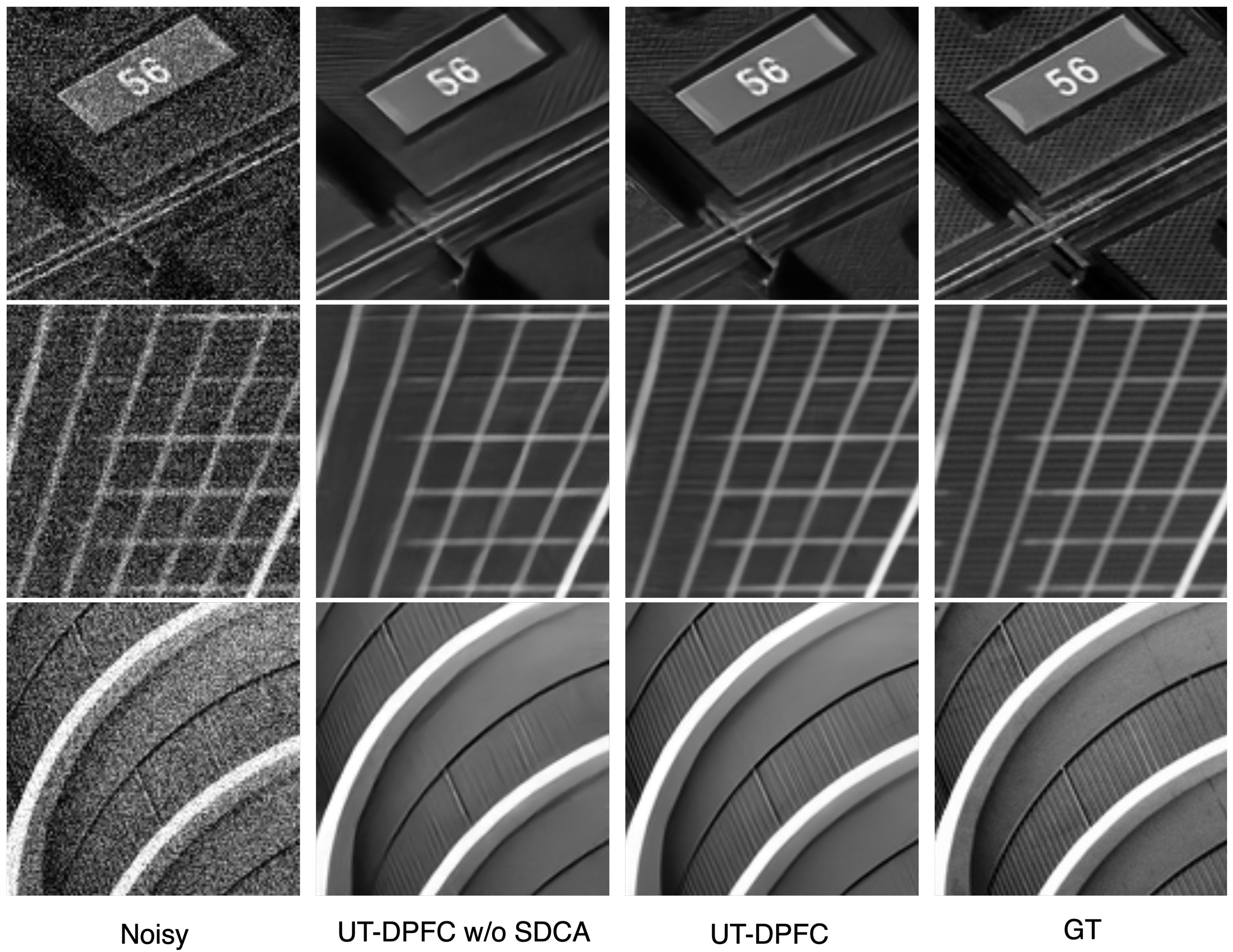
To provide an intuitive validation of the effectiveness of SDCA, we conducted a controlled ablation study under identical training and testing settings by comparing the backbone network without SDCA with the complete UT-DPFC model, together with their visual results. As shown in Figure 13, three representative local regions with heavy-noise and complex textures were presented. From left to right, the images correspond to the noisy input, the output of the backbone network without SDCA, the output of UT-DPFC, and the corresponding clean reference image. It could be observed that, although the backbone without SDCA suppressed noise effectively, fine details were more prone to over-smoothing and structural degradation. For example, in the first group, the fine textures around the digit “56” were smoothed out; in the second group, the thin-line structures became discontinuous; and in the third group, some railing details were lost. Removing SDCA loses the pre-fusion calibration ability, making the model vulnerable to noise interference and causing performance degradation especially under heavy noise. In contrast, after introducing SDCA, the restored details and structures were closer to those in the reference image while maintaining comparable noise suppression.

4.7.2. Ablation Study on the Insertion Position of the SDCA Module

To further investigate the effect of SDCA at different resolution levels, we conducted an ablation study on its insertion positions on the SIDD dataset. Specifically, while keeping the backbone architecture and training configuration unchanged, we compared the following settings: without SDCA, with SDCA inserted at a single-scale, at two scale combinations, at three scales, and at all four scales.

Table 8. Ablation results for different insertion scales of the SDCA module.

Insertion Scale	PSNR/dB	SSIM	MACs/G	Params/M
None	39.68	0.958	85.775	50.392
$H/2\times W/2$	39.86	0.959	90.750	50.680
$H/4\times W/4$	39.79	0.958	87.021	50.464
$H/8\times W/8$	39.74	0.958	86.088	50.410
$H/2\times W/2+H/4\times W/4$	39.94	0.960	91.995	50.752
$H/2\times W/2+H/8\times W/8$	39.91	0.959	91.062	50.698
$H/4\times W/4+H/8\times W/8$	39.86	0.959	87.333	50.482
UT-DPFC (Ours)	40.03	0.960	92.308	50.770
UT-DPFC (Ours)+ $H\times W$	40.05	0.960	112.189	51.920

reported the PSNR/SSIM results for each setting, together with the corresponding MACs and parameter counts, where the complexity statistics were measured with an input size of $256\times 256$.

The results indicated that the performance gains brought by single-scale insertion differed markedly across resolution levels. Compared with the baseline without SDCA, inserting SDCA only at the $H/2\times W/2$ level yielded the most pronounced improvement, with PSNR increasing by 0.18 dB and SSIM by 0.001. When SDCA was inserted only at the $H/4\times W/4$ and $H/8\times W/8$ levels, the PSNR gains were 0.11 dB and 0.06 dB, respectively. Furthermore, dual scale insertion led to further overall improvement. Among the dual scale settings, the combination of $H/2\times W/2$ and $H/4\times W/4$ outperformed the combinations of $H/2\times W/2+H/8\times W/8$ and $H/4\times W/4+H/8\times W/8$. When SDCA was inserted at three scales, the model achieved a further PSNR gain of 0.09 dB over the best dual scale setting, namely $H/2\times W/2+H/4\times W/4$. We further examined whether it was necessary to extend SDCA to the highest-resolution $H\times W$ level. The results showed that, based on the original UT-DPFC, additionally inserting SDCA at $H\times W$ brought only a marginal PSNR gain of 0.02 dB and no improvement in SSIM, while substantially increasing both computational cost and parameter count. Specifically, MACs increased by 19.881 G over 92.308 G, and the number of parameters increased by 1.150 M. Considering the above performance-efficiency trade-off, we finally adopted progressive decoder-side pre-fusion calibration at the three scales of $H/2$, $H/4$, and $H/8$, so as to achieve better overall performance while keeping the computational overhead controllable.

4.7.3. Ablation on the Main Components of UT-DPFC

To systematically verify the effectiveness of the main components in UT-DPFC, we conducted a component-wise ablation study under the same training and testing settings. The evaluated variants include removing SDCA, removing MSRC, removing MRPC, replacing MRPC with a plain convolutional structure, and replacing LeFF with a standard FFN. The corresponding PSNR, SSIM, MACs, and parameter counts are reported in

Table 9. Ablation results of the main components in UT-DPFC, including SDCA, MSRC, MRPC, and LeFF.

Models	PSNR (dB)	SSIM	MACs (G)	Params (M)
UT-DPFC $\mathrm{w}/\mathrm{o}\mathrm{SDCA}$	39.68	0.958	85.775	50.392
UT-DPFC $\mathrm{w}/\mathrm{o}\mathrm{MSRC}$	39.92	0.959	92.308	50.770
UT-DPFC $\mathrm{w}/\mathrm{o}\mathrm{MRPC}$	39.82	0.958	86.494	50.468
UT-DPFC ($\mathrm{MRPC}\to \mathrm{PlainConv}$)	39.89	0.959	92.308	50.770
UT-DPFC ($\mathrm{LeFF}\to \mathrm{FFN}$)	39.94	0.959	91.166	50.342
UT-DPFC (Ours)	40.03	0.960	92.308	50.770

.

For the variant without SDCA ($\mathrm{w}/\mathrm{o}\mathrm{SDCA}$), the decoder-side pre-fusion calibration module was removed, and the decoder features were directly used for subsequent encoder-decoder fusion. For the variant without MSRC ($\mathrm{w}/\mathrm{o}\mathrm{MSRC}$), the multi-scale region candidates were removed, while the remaining candidate construction was kept consistent as much as possible to evaluate the contribution of region-level structural cues. For the variant without MRPC ($\mathrm{w}/\mathrm{o}\mathrm{MRPC}$), the multi-receptive-field pixel candidates were removed and replaced with directly flattened projected features. Since directly removing MRPC also reduces the convolutional computation, we further constructed a computation-aligned variant ($\mathrm{MRPC}\to \mathrm{PlainConv}$), where the multi-receptive-field design was replaced with a plain convolutional structure while keeping the MACs and parameter count consistent with the full model. In addition, to evaluate the contribution of local enhancement in the Transformer block, we replaced LeFF with a standard feed-forward network ($\mathrm{LeFF}\to \mathrm{FFN}$).

As shown in Table 9, the full UT-DPFC achieved the best performance, with a PSNR of $40.03$ dB and an SSIM of $0.960$. Removing SDCA caused the most obvious degradation, reducing the PSNR from $40.03$ dB to $39.68$ dB. This result indicates that decoder-side pre-fusion calibration plays a critical role in improving the reliability of decoder representations before encoder-decoder fusion. When MSRC was removed, the PSNR decreased to $39.92$ dB, suggesting that multi-scale region candidates provide useful structural references for stable feature retrieval and aggregation. Removing MRPC led to a larger drop, with the PSNR decreasing to $39.82$ dB, which demonstrates the importance of multi-receptive-field pixel candidates for recovering fine-grained details such as edges and textures.

Furthermore, the $\mathrm{MRPC}\to \mathrm{PlainConv}$ variant achieved a PSNR of $39.89$ dB under the same MACs and parameter count as the full model, which rules out the possibility that the improvement comes merely from increased computation. This comparison further verifies that the multi-receptive-field design in MRPC is more effective than a plain convolutional alternative for constructing detail-sensitive pixel candidates. Replacing LeFF with a standard FFN also reduced the PSNR from $40.03$ dB to $39.94$ dB, indicating that the locally enhanced feed-forward design contributes to local detail modeling. Overall, these ablation results demonstrate that SDCA is the primary contributor to the performance improvement, while MSRC, MRPC, and LeFF further enhance structural robustness, fine-detail restoration, and local feature representation, respectively.

4.7.4. Hyperparameter Analysis

To further examine the influence of key hyperparameter settings, we conducted a series of controlled experiments, as reported in

Table 10. Hyperparameter analysis of the number of Transformer blocks.

Number of Transformer Blocks	Params (M)	MACs (G)	PSNR (dB)
$\{1,2,6,6,2\}$	40.80	75.418	39.86
$\{1,2,8,8,2\}$	50.77	92.308	40.03
$\{1,2,10,10,2\}$	60.74	109.198	39.98

,

Table 11. Hyperparameter analysis of the channel reduction ratio $\rho$.

Reduction Ratio $\mathsf{\rho }$	Params (M)	MACs (G)	PSNR (dB)
1	51.93	123.208	39.92
2	50.77	92.308	40.03
4	50.47	79.168	39.87

,

Table 12. Effect of different MSRC scale combinations on model complexity and denoising performance.

MSRC Scale Combination	Params (M)	MACs (G)	PSNR (dB)
$\{2,3,4,5\}$	50.77	92.858	39.93
$\{2,3,5,6\}$	50.77	92.308	40.03
$\{2,4,6,8\}$	50.77	91.313	39.95

and

Table 13. Effect of different MRPC multi-receptive-field branch designs on model complexity and denoising performance.

Connection Type	Branch Design	Params (M)	MACs (G)	PSNR (dB)
Parallel	$C_1\left(X\right),C_3\left(X\right)$	50.41	89.318	39.84
Parallel	$C_1\left(X\right),C_3\left(X\right),C_5\left(X\right)$	50.68	91.518	39.88
Cascaded	$C_1\left(X\right),C_3\left(X\right),C_3\left(C_1\left(X\right)\right)$	50.50	90.108	39.93
Cascaded	$C_1\left(X\right),C_3\left(X\right),C_3\left(C_1\left(X\right)\right),C_5\left(C_3\left(C_1\left(X\right)\right)\right)$	50.77	92.308	40.03

. First, Table 10 shows the effect of different Transformer block configurations. When the block configuration is increased from $\{1, 2, 6, 6, 2\}$ to $\{1, 2, 8, 8, 2\}$, the PSNR improves from 39.86 dB to 40.03 dB, indicating that a moderate increase in model depth can enhance the representation capability of the network. However, further increasing the configuration to $\{1, 2, 10, 10, 2\}$ raises the parameter count and MACs to 60.74 M and 109.198 G, respectively, while the PSNR slightly decreases to 39.98 dB. This suggests that excessive depth may introduce redundant computation and does not necessarily lead to better denoising performance. Therefore, $\{1, 2, 8, 8, 2\}$ is adopted as the final Transformer block configuration.

Table 11 analyzes the influence of the channel reduction ratio $\rho$. Compared with $\rho =1$, setting $\rho =2$ reduces the computational cost from 123.208 G to 92.308 G while improving the PSNR from 39.92 dB to 40.03 dB. When $\rho$ is further increased to 4, the MACs are reduced to 79.168 G, but the PSNR drops to 39.87 dB, indicating that overly aggressive channel reduction weakens feature representation. Thus, $\rho =2$ provides a better balance between computational efficiency and restoration accuracy.

Table 12 further compares different MSRC scale combinations. The setting $\{2, 3, 5, 6\}$ achieves the best PSNR of 40.03 dB, outperforming $\{2, 3, 4, 5\}$ and $\{2, 4, 6, 8\}$. This result suggests that combining adjacent and moderately enlarged pooling scales provides more effective multi-scale regional context for denoising.

Finally, Table 13 evaluates different MRPC multi-receptive-field branch designs. The results show that cascaded branch designs perform better than simple parallel designs. In particular, the cascaded configuration $C_1\left(X\right),C_3\left(X\right),C_3\left(C_1\left(X\right)\right),C_5\left(C_3\left(C_1\left(X\right)\right)\right)$ achieves the highest PSNR of 40.03 dB, while maintaining a moderate computational cost of 92.308 G MACs. This indicates that progressively expanding the receptive field can provide more complementary pixel-level detail responses than directly parallel convolutional branches. Overall, these hyperparameter studies verify the rationality of the adopted settings and demonstrate that the final configuration achieves a favorable trade-off among parameter count, computational cost, and denoising performance.

5. Conclusions and Future Work

To address the limitation of lacking pre-fusion calibration in existing U-shaped Transformer denoising models, we propose UT-DPFC with decoder-side pre-fusion calibration, which is a novel design for U-shaped Transformer-based image restoration. Built on a U-shaped Transformer backbone, the proposed network introduces SDCA before encoder-decoder fusion at three decoding levels to calibrate decoder features prior to fusion. Specifically, SDCA generates queries from decoder features and performs content-adaptive retrieval and aggregation over two complementary candidate pools, namely MSRC for structural cues and MRPC for detail cues, thereby improving the reliability of the fusion basis and supporting more stable detail reconstruction. Extensive experiments verify the effectiveness of UT-DPFC from multiple dimensions. Firstly, on real-world denoising benchmarks (SIDD, DND) and synthetic AWGN denoising tasks, quantitative results demonstrate that our method achieves consistent performance improvements in PSNR and SSIM compared with mainstream existing approaches. Secondly, fine-grained regional error analysis confirms that our method exhibits superior detail restoration ability in challenging regions with heavy noise and rich textures, which accounts for the overall performance gains. Thirdly, efficiency analysis reveals that the performance improvement is achieved without excessive computational cost, maintaining a moderate and affordable computational burden. Finally, comprehensive ablation studies, including the ablation of core components of UT-DPFC and the SDCA module as well as hyperparameter analysis, validate the necessity of each design and prove the robustness of the proposed framework to key hyperparameters. In summary, UT-DPFC serves as a reliable, efficient and stable solution for image denoising.

In future work, we will explore extending the proposed decoder-side pre-fusion calibration strategy to other image restoration tasks, such as deraining, dehazing, and deblurring, to further validate its generality and transferability.

References

1. Ronghui, L.; Chen, T.J. Research on image segmentation effect based on denoising preprocessing. J. Electron. Imaging 2024, 33, 033033. [Google Scholar] [CrossRef]
2. Song, M.; Li, L.; Yu, X.; Chen, C. Pushing the boundaries of salient object detection: A denoising-driven approach. IEEE Trans. Image Process. 2025, 34, 3903–3917. [Google Scholar] [CrossRef] [PubMed]
3. Lee, T.; Lee, S.; Kwon, H. Dual-targeted adversarial noise for 3D point cloud classification model. Sci. Rep. 2025, 15, 42566. [Google Scholar] [CrossRef] [PubMed]
4. Kwon, H. Inducing divergent misclassifications: Dual-targeted adversarial attacks on video recognition models. Mach. Vis. Appl. 2026, 37, 33. [Google Scholar] [CrossRef]
5. Lee, T.; Lee, S.; Kwon, H. Comrade-Secure Adversarial Noise for 3D Point Cloud Classification Model. IET Image Process. 2025, 19, e70215. [Google Scholar] [CrossRef]
6. Cai, R.; Chen, G.; Li, J.; Du, R.; Lu, H.; Qi, Y.; Chen, J. A denoising method for salt and pepper noise in remote sensing based on Swin-Transformer convolution U-Net and filtering—FSCU-Net. Earth Space Sci. 2025, 12, e2025EA004225. [Google Scholar] [CrossRef]
7. Wang, S.; Fan, X.; Zhao, Z.; Qiao, Z.; Wang, N.; Qiu, Y.; Jia, X. Research on steel surface defect detection system based on YOLOv5s-SE-CA model and BEMD image enhancement. Nondestruct. Test. Eval. 2025, 40, 3080–3099. [Google Scholar] [CrossRef]
8. Zhang, J.; Gong, W.; Ye, L.; Wang, F.; Shangguan, Z.; Cheng, Y. A review of deep learning methods for denoising of medical low-dose CT images. Comput. Biol. Med. 2024, 171, 108112. [Google Scholar] [CrossRef] [PubMed]
9. Volkov, A.A.; Kozlov, A.V.; Cheremkhin, P.A.; Rymov, D.A.; Shifrina, A.V.; Starikov, R.S.; Nebavskiy, V.A.; Petrova, E.K.; Zlokazov, E.Y.; Rodin, V.G. A review of Neural network-based image noise processing methods. Sensors 2025, 25, 6088. [Google Scholar] [CrossRef]
10. Aharon, M.; Elad, M.; Bruckstein, A. K-SVD: An algorithm for designing overcomplete dictionaries for sparse representation. IEEE Trans. Signal Process. 2006, 54, 4311–4322. [Google Scholar] [CrossRef]
11. Buades, A.; Coll, B.; Morel, J.M. A non-local algorithm for image denoising. In Proceedings of the 2005 IEEE Computer Society Conference on Computer Vision and Pattern Recognition (CVPR’05); IEEE: Piscataway, NJ, USA, 2005; Volume 2, pp. 60–65. [Google Scholar]
12. Dabov, K.; Foi, A.; Katkovnik, V.; Egiazarian, K. Image denoising by sparse 3-D transform-domain collaborative filtering. IEEE Trans. Image Process. 2007, 16, 2080–2095. [Google Scholar] [CrossRef]
13. Mao, J.; Sun, L.; Chen, J.; Yu, S. Overview of research on digital image denoising methods. Sensors 2025, 25, 2615. [Google Scholar] [CrossRef]
14. Zhang, K.; Zuo, W.; Chen, Y.; Meng, D.; Zhang, L. Beyond a gaussian denoiser: Residual learning of deep cnn for image denoising. IEEE Trans. Image Process. 2017, 26, 3142–3155. [Google Scholar] [CrossRef] [PubMed]
15. Zhang, K.; Zuo, W.; Zhang, L. FFDNet: Toward a fast and flexible solution for CNN-based image denoising. IEEE Trans. Image Process. 2018, 27, 4608–4622. [Google Scholar] [CrossRef]
16. Guo, S.; Yan, Z.; Zhang, K.; Zuo, W.; Zhang, L. Toward convolutional blind denoising of real photographs. In Proceedings of the IEEE/CVF Conference on Computer Vision and Pattern Recognition; IEEE: Piscataway, NJ, USA, 2019; pp. 1712–1722. [Google Scholar]
17. Yu, S.; Park, B.; Jeong, J. Deep iterative down-up cnn for image denoising. In Proceedings of the IEEE/CVF Conference on Computer Vision and Pattern Recognition Workshops; IEEE: Piscataway, NJ, USA, 2019. [Google Scholar]
18. Zhang, K.; Li, Y.; Zuo, W.; Zhang, L.; Van Gool, L.; Timofte, R. Plug-and-play image restoration with deep denoiser prior. IEEE Trans. Pattern Anal. Mach. Intell. 2021, 44, 6360–6376. [Google Scholar] [CrossRef] [PubMed]
19. Ronneberger, O.; Fischer, P.; Brox, T. U-net: Convolutional networks for biomedical image segmentation. In Proceedings of the International Conference on Medical Image Computing and Computer-Assisted Intervention; Springer: Berlin/Heidelberg, Germany, 2015; pp. 234–241. [Google Scholar]
20. Vaswani, A.; Shazeer, N.; Parmar, N.; Uszkoreit, J.; Jones, L.; Gomez, A.N.; Kaiser, Ł.; Polosukhin, I. Attention is all you need. Adv. Neural Inf. Process. Syst. 2017, 30, 5998–6008. [Google Scholar]
21. Chen, H.; Wang, Y.; Guo, T.; Xu, C.; Deng, Y.; Liu, Z.; Ma, S.; Xu, C.; Xu, C.; Gao, W. Pre-trained image processing transformer. In Proceedings of the IEEE/CVF Conference on Computer Vision and Pattern Recognition; IEEE: Piscataway, NJ, USA, 2021; pp. 12299–12310. [Google Scholar]
22. Liang, J.; Cao, J.; Sun, G.; Zhang, K.; Van Gool, L.; Timofte, R. Swinir: Image restoration using swin transformer. In Proceedings of the IEEE/CVF International Conference on Computer Vision; IEEE: Piscataway, NJ, USA, 2021; pp. 1833–1844. [Google Scholar]
23. Wang, Z.; Cun, X.; Bao, J.; Zhou, W.; Liu, J.; Li, H. Uformer: A general u-shaped transformer for image restoration. In Proceedings of the IEEE/CVF Conference on Computer Vision and Pattern Recognition; IEEE: Piscataway, NJ, USA, 2022; pp. 17683–17693. [Google Scholar]
24. Fan, C.M.; Liu, T.J.; Liu, K.H. SUNet: Swin transformer UNet for image denoising. In Proceedings of the 2022 IEEE International Symposium on Circuits And Systems (ISCAS); IEEE: Piscataway, NJ, USA, 2022; pp. 2333–2337. [Google Scholar]
25. Zamir, S.W.; Arora, A.; Khan, S.; Hayat, M.; Khan, F.S.; Yang, M.H. Restormer: Efficient transformer for high-resolution image restoration. In Proceedings of the IEEE/CVF Conference on Computer Vision and Pattern Recognition; IEEE: Piscataway, NJ, USA, 2022; pp. 5728–5739. [Google Scholar]
26. Gao, H.; Dang, D. Exploring richer and more accurate information via frequency selection for image restoration. IEEE Trans. Circuits Syst. Video Technol. 2024, 35, 2689–2700. [Google Scholar] [CrossRef]
27. Gao, H.; Lei, X.; Dang, D. Enhancing image restoration through learning context-rich and detail-accurate features. Neural Netw. 2025, 194, 108096. [Google Scholar] [CrossRef]
28. Chen, L.; Chu, X.; Zhang, X.; Sun, J. Simple baselines for image restoration. In Proceedings of the European Conference on Computer Vision; Springer: Berlin/Heidelberg, Germany, 2022; pp. 17–33. [Google Scholar]
29. Lin, Y.C.; Xu, Y.S.; Chen, H.W.; Kuo, H.K.; Lee, C.Y. Eamamba: Efficient all-around vision state space model for image restoration. In Proceedings of the IEEE/CVF International Conference on Computer Vision; IEEE: Piscataway, NJ, USA, 2025; pp. 11708–11719. [Google Scholar]
30. Zhang, Y.; Yu, H.; Yang, Y.; Liu, J.; Li, Q.; Huang, Z. FUT: Frequency-aware U-shaped transformer for image denoising. J. Vis. Commun. Image Represent. 2025, 111, 104528. [Google Scholar] [CrossRef]
31. Huang, Z.; Yang, Y.; Liu, J.; Liu, C.; Shi, Y.; Zhang, Y.; Li, Q. RUST: Residual U-shaped transformer to approximate Taylor expansion for image denoising. Knowl.-Based Syst. 2025, 330, 114593. [Google Scholar] [CrossRef]
32. Boucherit, I.; Kheddar, H. Reinforced residual encoder–decoder network for image denoising via deeper encoding and balanced skip connections. Big Data Cogn. Comput. 2025, 9, 82. [Google Scholar] [CrossRef]
33. Wang, X.; Girshick, R.; Gupta, A.; He, K. Non-local neural networks. In Proceedings of the IEEE Conference on Computer Vision and Pattern Recognition; IEEE: Piscataway, NJ, USA, 2018; pp. 7794–7803. [Google Scholar]
34. Liu, D.; Wen, B.; Fan, Y.; Loy, C.C.; Huang, T.S. Non-local recurrent network for image restoration. Adv. Neural Inf. Process. Syst. 2018, 31, 1673–1682. [Google Scholar]
35. Zhang, Y.; Li, K.; Li, K.; Zhong, B.; Fu, Y. Residual non-local attention networks for image restoration. arXiv 2019, arXiv:1903.10082. [Google Scholar] [CrossRef]
36. Hu, Y.; Cheng, D.; Huang, Z.; Chen, B.; Lin, S.; Zhang, S. DSCA-former: Dual-stem cross-attentive transformer for image denoising. Neurocomputing 2026, 671, 132656. [Google Scholar] [CrossRef]
37. He, K.; Zhang, X.; Ren, S.; Sun, J. Spatial pyramid pooling in deep convolutional networks for visual recognition. IEEE Trans. Pattern Anal. Mach. Intell. 2015, 37, 1904–1916. [Google Scholar] [CrossRef]
38. Chen, L.C.; Papandreou, G.; Kokkinos, I.; Murphy, K.; Yuille, A.L. Deeplab: Semantic image segmentation with deep convolutional nets, atrous convolution, and fully connected crfs. IEEE Trans. Pattern Anal. Mach. Intell. 2017, 40, 834–848. [Google Scholar] [CrossRef]
39. Zhao, Y.; Jiang, Z.; Men, A.; Ju, G. Pyramid real image denoising network. In Proceedings of the 2019 IEEE Visual Communications and Image Processing (VCIP); IEEE: Piscataway, NJ, USA, 2019; pp. 1–4. [Google Scholar]
40. Jia, X.; Peng, Y.; Li, J.; Xin, Y.; Ge, B.; Liu, S. Pyramid dilated convolutional neural network for image denoising. J. Electron. Imaging 2022, 31, 023024. [Google Scholar] [CrossRef]
41. Duong, M.T.; Nguyen Thi, B.T.; Lee, S.; Hong, M.C. Multi-branch network for color image denoising using dilated convolution and attention mechanisms. Sensors 2024, 24, 3608. [Google Scholar] [CrossRef]
42. Timofte, R.; Agustsson, E.; Van Gool, L.; Yang, M.H.; Zhang, L. Ntire 2017 challenge on single image super-resolution: Methods and results. In Proceedings of the IEEE Conference on Computer Vision and Pattern Recognition Workshops; IEEE: Piscataway, NJ, USA, 2017; pp. 114–125. [Google Scholar]
43. Lim, B.; Son, S.; Kim, H.; Nah, S.; Mu Lee, K. Enhanced deep residual networks for single image super-resolution. In Proceedings of the IEEE Conference on Computer Vision and Pattern Recognition Workshops; IEEE: Piscataway, NJ, USA, 2017; pp. 136–144. [Google Scholar]
44. Ma, K.; Duanmu, Z.; Wu, Q.; Wang, Z.; Yong, H.; Li, H.; Zhang, L. Waterloo exploration database: New challenges for image quality assessment models. IEEE Trans. Image Process. 2016, 26, 1004–1016. [Google Scholar] [CrossRef]
45. Martin, D.; Fowlkes, C.; Tal, D.; Malik, J. A database of human segmented natural images and its application to evaluating segmentation algorithms and measuring ecological statistics. In Proceedings of the Eighth IEEE International Conference on Computer Vision; ICCV 2001; IEEE: Piscataway, NJ, USA, 2001; Volume 2, pp. 416–423. [Google Scholar]
46. Huang, J.B.; Singh, A.; Ahuja, N. Single image super-resolution from transformed self-exemplars. In Proceedings of the IEEE Conference on Computer Vision and Pattern Recognition; IEEE: Piscataway, NJ, USA, 2015; pp. 5197–5206. [Google Scholar]
47. Franzen, R. Kodak Lossless True Color Image Suite. Available online: https://r0k.us/graphics/kodak/ (accessed on 10 March 2026).
48. Zhang, L.; Wu, X.; Buades, A.; Li, X. Color demosaicking by local directional interpolation and nonlocal adaptive thresholding. J. Electron. Imaging 2011, 20, 023016. [Google Scholar] [CrossRef]
49. Abdelhamed, A.; Lin, S.; Brown, M.S. A high-quality denoising dataset for smartphone cameras. In Proceedings of the IEEE Conference on Computer Vision and Pattern Recognition; IEEE: Piscataway, NJ, USA, 2018; pp. 1692–1700. [Google Scholar]
50. Plotz, T.; Roth, S. Benchmarking denoising algorithms with real photographs. In Proceedings of the IEEE Conference on Computer Vision and Pattern Recognition; IEEE: Piscataway, NJ, USA, 2017; pp. 1586–1595. [Google Scholar]
51. Hore, A.; Ziou, D. Image quality metrics: PSNR vs. SSIM. In Proceedings of the 2010 20th International Conference on Pattern Recognition; IEEE: Piscataway, NJ, USA, 2010; pp. 2366–2369. [Google Scholar]
52. Wang, Z.; Bovik, A.C.; Sheikh, H.R.; Simoncelli, E.P. Image quality assessment: From error visibility to structural similarity. IEEE Trans. Image Process. 2004, 13, 600–612. [Google Scholar] [CrossRef]
53. Liu, P.; Zhang, H.; Zhang, K.; Lin, L.; Zuo, W. Multi-level wavelet-CNN for image restoration. In Proceedings of the IEEE Conference on Computer Vision and Pattern Recognition Workshops; IEEE: Piscataway, NJ, USA, 2018; pp. 773–782. [Google Scholar]
54. Zhang, K.; Li, Y.; Liang, J.; Cao, J.; Zhang, Y.; Tang, H.; Fan, D.P.; Timofte, R.; Gool, L.V. Practical blind image denoising via Swin-Conv-UNet and data synthesis. Mach. Intell. Res. 2023, 20, 822–836. [Google Scholar] [CrossRef]
55. Zhang, Y.; Li, D.; Shi, X.; He, D.; Song, K.; Wang, X.; Qin, H.; Li, H. Kbnet: Kernel basis network for image restoration. arXiv 2023, arXiv:2303.02881. [Google Scholar] [CrossRef]
56. Ghasemabadi, A.; Janjua, M.K.; Salameh, M.; Zhou, C.; Sun, F.; Niu, D. Cascadedgaze: Efficiency in global context extraction for image restoration. arXiv 2024, arXiv:2401.15235. [Google Scholar] [CrossRef]
57. Anwar, S.; Barnes, N. Real image denoising with feature attention. In Proceedings of the IEEE/CVF International Conference on Computer Vision; IEEE: Piscataway, NJ, USA, 2019; pp. 3155–3164. [Google Scholar]
58. Kim, Y.; Soh, J.W.; Park, G.Y.; Cho, N.I. Transfer learning from synthetic to real-noise denoising with adaptive instance normalization. In Proceedings of the IEEE/CVF Conference on Computer Vision and Pattern Recognition; IEEE: Piscataway, NJ, USA, 2020; pp. 3482–3492. [Google Scholar]
59. Zamir, S.W.; Arora, A.; Khan, S.; Hayat, M.; Khan, F.S.; Yang, M.H.; Shao, L. Cycleisp: Real image restoration via improved data synthesis. In Proceedings of the IEEE/CVF Conference on Computer Vision and Pattern Recognition; IEEE: Piscataway, NJ, USA, 2020; pp. 2696–2705. [Google Scholar]
60. Zamir, S.W.; Arora, A.; Khan, S.; Hayat, M.; Khan, F.S.; Yang, M.H.; Shao, L. Learning enriched features for real image restoration and enhancement. In Proceedings of the European Conference on Computer Vision; Springer: Berlin/Heidelberg, Germany, 2020; pp. 492–511. [Google Scholar]
61. Zamir, S.W.; Arora, A.; Khan, S.; Hayat, M.; Khan, F.S.; Yang, M.H.; Shao, L. Multi-stage progressive image restoration. In Proceedings of the IEEE/CVF Conference on Computer Vision and Pattern Recognition; IEEE: Piscataway, NJ, USA, 2021; pp. 14821–14831. [Google Scholar]
62. Zhang, J.; Zhang, Y.; Gu, J.; Dong, J.; Kong, L.; Yang, X. Xformer: Hybrid x-shaped transformer for image denoising. arXiv 2023, arXiv:2303.06440. [Google Scholar]
63. Guo, H.; Li, J.; Dai, T.; Ouyang, Z.; Ren, X.; Xia, S.T. Mambair: A simple baseline for image restoration with state-space model. In Proceedings of the European Conference on Computer Vision; Springer: Berlin/Heidelberg, Germany, 2024; pp. 222–241. [Google Scholar]
64. Wu, W.; Liu, S.; Xia, Y.; Zhang, Y. Dual residual attention network for image denoising. Pattern Recognit. 2024, 149, 110291. [Google Scholar] [CrossRef]
65. Brateanu, A.; Balmez, R.; Avram, A.; Orhei, C. Akdt: Adaptive kernel dilation transformer for effective image denoising. Proc. Copyr. 2025, 418, 19. [Google Scholar]
66. Xu, J.; Zhang, L.; Zhang, D.; Feng, X. Multi-channel weighted nuclear norm minimization for real color image denoising. In Proceedings of the IEEE International Conference on Computer Vision; IEEE: Piscataway, NJ, USA, 2017; pp. 1096–1104. [Google Scholar]
67. Zhang, K.; Zuo, W.; Gu, S.; Zhang, L. Learning deep CNN denoiser prior for image restoration. In Proceedings of the IEEE Conference on Computer Vision and Pattern Recognition; IEEE: Piscataway, NJ, USA, 2017; pp. 3929–3938. [Google Scholar]
68. Tian, C.; Xu, Y.; Li, Z.; Zuo, W.; Fei, L.; Liu, H. Attention-guided CNN for image denoising. Neural Netw. 2020, 124, 117–129. [Google Scholar] [CrossRef]
69. Chang, M.; Li, Q.; Feng, H.; Xu, Z. Spatial-adaptive network for single image denoising. In Proceedings of the European Conference on Computer Vision; Springer: Berlin/Heidelberg, Germany, 2020; pp. 171–187. [Google Scholar]
70. Li, B.; Liu, X.; Hu, P.; Wu, Z.; Lv, J.; Peng, X. All-in-one image restoration for unknown corruption. In Proceedings of the IEEE/CVF Conference on Computer Vision and Pattern Recognition; IEEE: Piscataway, NJ, USA, 2022; pp. 17452–17462. [Google Scholar]
Figure 1. The architecture of the proposed UT-DPFC network.
Applsci 16 04523 g001
Figure 2. The architecture of the SDCA module.
Applsci 16 04523 g002
Figure 3. Structural illustrations of the MSRC and MRPC modules using a 7 × 7 feature map as an example.
Applsci 16 04523 g003
Figure 4. Visual comparison of different methods on Gaussian grayscale image denoising over the Urban100 dataset ( σ = 50 ).
Applsci 16 04523 g004
Figure 5. Visual comparison of different methods on Gaussian grayscale image denoising over the Set12 dataset ( σ = 25 ).
Applsci 16 04523 g005
Figure 6. Visual comparison of different methods on Gaussian color image denoising over the Urban100 dataset ( σ = 50 ).
Applsci 16 04523 g006
Figure 7. Visual comparison of different methods on Gaussian color image denoising over the McMaster68 dataset ( σ = 25 ).
Applsci 16 04523 g007
Figure 8. PSNR-MACs comparison of different methods including Restormer [25] , DRUNet [18], KBNet [55], DnCNN [14], RNAN [35] and SwinIR [22] for Gaussian denoising on the Urban100 dataset ( σ = 50 ). (Left): Grayscale image denoising; (Right): Color image denoising.
Applsci 16 04523 g008
Figure 9. Visual comparison of different methods for real-world image denoising on the SIDD dataset.
Applsci 16 04523 g009
Figure 10. PSNR-MACs comparison of different methods including Restormer [25], Uformer [23], EAMamba [29], AKDT [65], CycleISP [59], MPRNet [61] and MIRNet [60] for real-world image denoising on the SIDD dataset.
Applsci 16 04523 g010
Figure 11. Visual results on the DND dataset. (The noisy images are shown in the top row, and the corresponding denoised images are shown in the bottom row).
Applsci 16 04523 g011
Figure 12. Region-wise error visualization comparison on Urban100 with σ = 50 .
Applsci 16 04523 g012
Figure 13. Ablation study results of the proposed UT-DPFC method on key components.
Applsci 16 04523 g013