Eigenbeam–vMF-Based Room Acoustic Analyzer: A Comparative Study with First-Order and Higher-Order Ambisonic Recordings

Abstract

Comprehensive room acoustic characterization requires resolving reflection behavior across time, frequency, and space. The recently proposed eigenbeam–vMF-based analyzer provides a framework for this by modeling the reflection field as a time–frequency-dependent directional power distribution, estimated via spatial correlation of eigenbeams (ambisonics) and parameterized using von Mises–Fisher clustering. This formulation enables a unified and interpretable description of anisotropic early reflections, their transition into diffuse reverberation, and frequency-dependent acoustic behavior. Prior work showed that the analyzer reliably captures these features using higher-order ambisonics from a 32-channel spherical microphone array (SMA) and that constraining the same array to the first order still led to retaining the dominant features. This paper investigates whether this capability extends to first-order microphone arrays with sparser spatial sampling for more economical and practical deployment. A comparative study is conducted in a recording studio with variable wall panels (wood and felt), evaluating a four-channel first-order array against a 32-channel SMA. The results reveal distinct acoustic differences between panel settings, which are consistent across both arrays. While the SMA captures finer spatial detail and prolonged anisotropic reflections more effectively, the first-order array demonstrates potential for preliminary room acoustic assessments by identifying room mode frequencies, dominant reflection directions, and highly reflective surfaces.

1. Introduction

Room acoustic analysis is essential for understanding how sound propagates, reflects, and decays within an environment. These characteristics directly influence both the physical sound field and human perception, their estimation fundamental for applications ranging from spatial audio rendering and machine hearing systems to architectural design.

The characterization of room acoustics evolved from Sabine’s reverberation time formulation [1] to a broader framework incorporating parameters such as clarity, definition, early decay time, and the direct-to-reverberant ratio [2,3]. Beyond these, a reliable understanding of room acoustic behavior requires a multi-dimensional analysis involving the spatial, temporal, and spectral features of reflections. While computational models [4] are widely used to predict acoustic behavior based on geometric information, their reliance on simplified assumptions regarding surface properties, wave interactions, and source–receiver properties can lead to significant deviations from actual acoustic behavior.

Sound field measurements using microphone arrays provide direct access to the acoustic field, enabling detailed analysis of the reflection structure. Early studies employed beamforming [5] and intensity vector analysis [6,7] for directional characterization and localization of reflections, while later approaches leveraged correlation and covariance of array measurements for improved spatial sensitivity [8,9].

The introduction of ambisonic microphone arrays led to the development of advanced methods for high-resolution spatial analysis utilizing spherical harmonic (SH) domain representation of the sound field [10,11,12,13]. Tools such as IRIS facilitate the temporal analysis of early and late reflections in terms of magnitude and direction using first-order ambisonic measurements [14]. Many methods employ plane wave decomposition in the SH domain to estimate the directions of arrival of early reflections [15,16] and to analyze the anisotropic characteristics of late reverberant fields [17,18,19,20]. Further developments using subspace processing [21] and correlation of higher-order ambisonics (eigenbeams) [22,23,24] achieved improved spatial accuracy and robustness to noise. Most of these methods rely on spherical microphone arrays (SMAs) to achieve accurate characterization of 3D spatial information. However, despite these advances, existing approaches generally lack a structured and interpretable directional representation that can unify the characterization of early and late reflections, particularly in capturing their frequency-dependent behavior.

To address this limitation, we introduced a room acoustic analyzer in [25] that models the reflection field as a time–frequency-dependent directional power distribution, enabling coherent analysis across different reflection regimes. This formulation captures variations in reflection gain due to non-homogeneous room surfaces, along with the temporal evolution of the non-diffuse sound field. The analyzer first employs eigenbeam-based spatial correlation to estimate the directional power of reflections separated from the direct sound component. A von Mises–Fisher (vMF) mixture model is then applied to parameterize the directional structure and distinguish anisotropic reflections. Using higher-order eigenbeams derived from a 32-channel SMA measurement, this framework has been validated to capture key acoustic behaviors, including frequency-dependent modal activity, the transition from anisotropic early reflections to diffuse late reverberation, source-dependent dominant reflection directions, and the association of long decay times with highly reflective surfaces. While this multifaceted characterization is effective, practical deployment using higher-order microphone arrays may not be cost-effective or accessible.

More economical alternatives, such as first-order ambisonic (B-format) microphone arrays [26,27,28], though widely available, find limited use in room acoustic analysis due to inherent spatial constraints. The sparse sampling and restriction to first-order SH representation reduce the angular resolution in 3D analysis. As a result, these arrays struggle to resolve real-world reflection fields, which are typically non-diffuse and exhibit a complex directional structure. Additionally, they are constrained by a low spatial aliasing frequency (typically around 1–3 kHz, depending on the inter-capsule spacing), limiting their ability to capture spatial variations at higher frequencies. Such effects were observed in [29], where traditional B-format microphones exhibited less stable performance across frequencies, along with increased angular scatter at low frequencies, indicating reduced directional precision. While prior work [25] suggests that certain acoustic features can be extracted from order-reduced representations derived from densely sampled arrays, it remains unclear whether faithful spatial characterization of room reflections across temporal and frequency dimensions can be achieved using a native first-order microphone array.

1.1. Approach and Contribution

In this paper, we investigate the viability of a first-order microphone array for reliable room acoustic characterization by applying the eigenbeam–vMF-based analyzer [25]. To this end, we conduct a comparative study with a higher-order SMA in a recording studio with variable acoustic configurations.

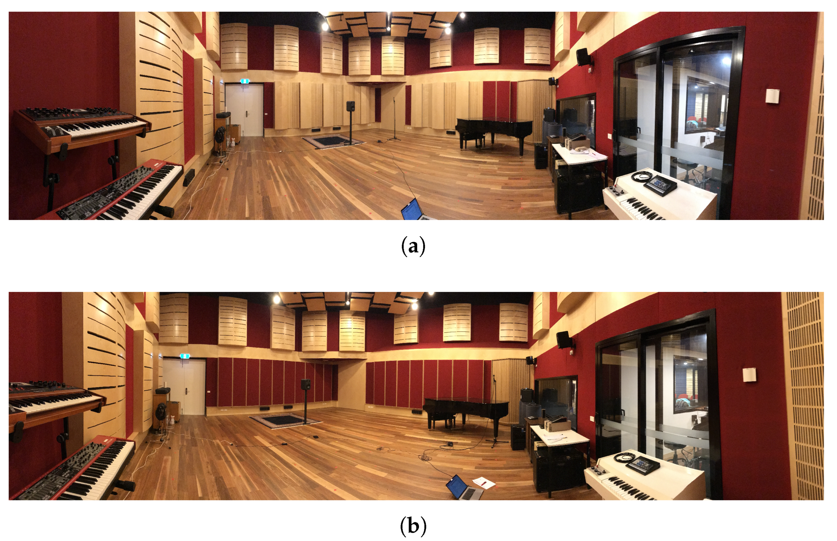
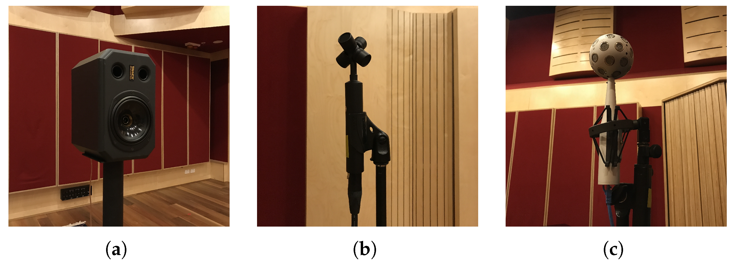
The recording studio features variable wall panels with wood and felt materials on two adjacent walls, allowing us to examine two acoustic configurations: all panels set to wood or felt. By applying the analyzer, we examine the variations in acoustic features between these configurations using two distinct microphone arrays: a 32-channel SMA (mh acoustics EM32 Eigenmike) and a 4-channel first-order microphone array (Rode NT-SF1). The comparative study includes an analysis of the spectral response of the reflection power, dominant reflection directions, directivity time-span, and directional decay time.

The results show that while the SMA captures finer spatial detail, the first-order array is able to identify essential acoustic features and distinguish between the two acoustic configurations. This indicates the suitability of first-order arrays for preliminary room acoustic analysis in cost-constrained scenarios and highlights the potential to extend this approach to consumer-grade devices, enabling more resource-efficient and scalable measurement set-ups.

1.2. Organization of the Paper

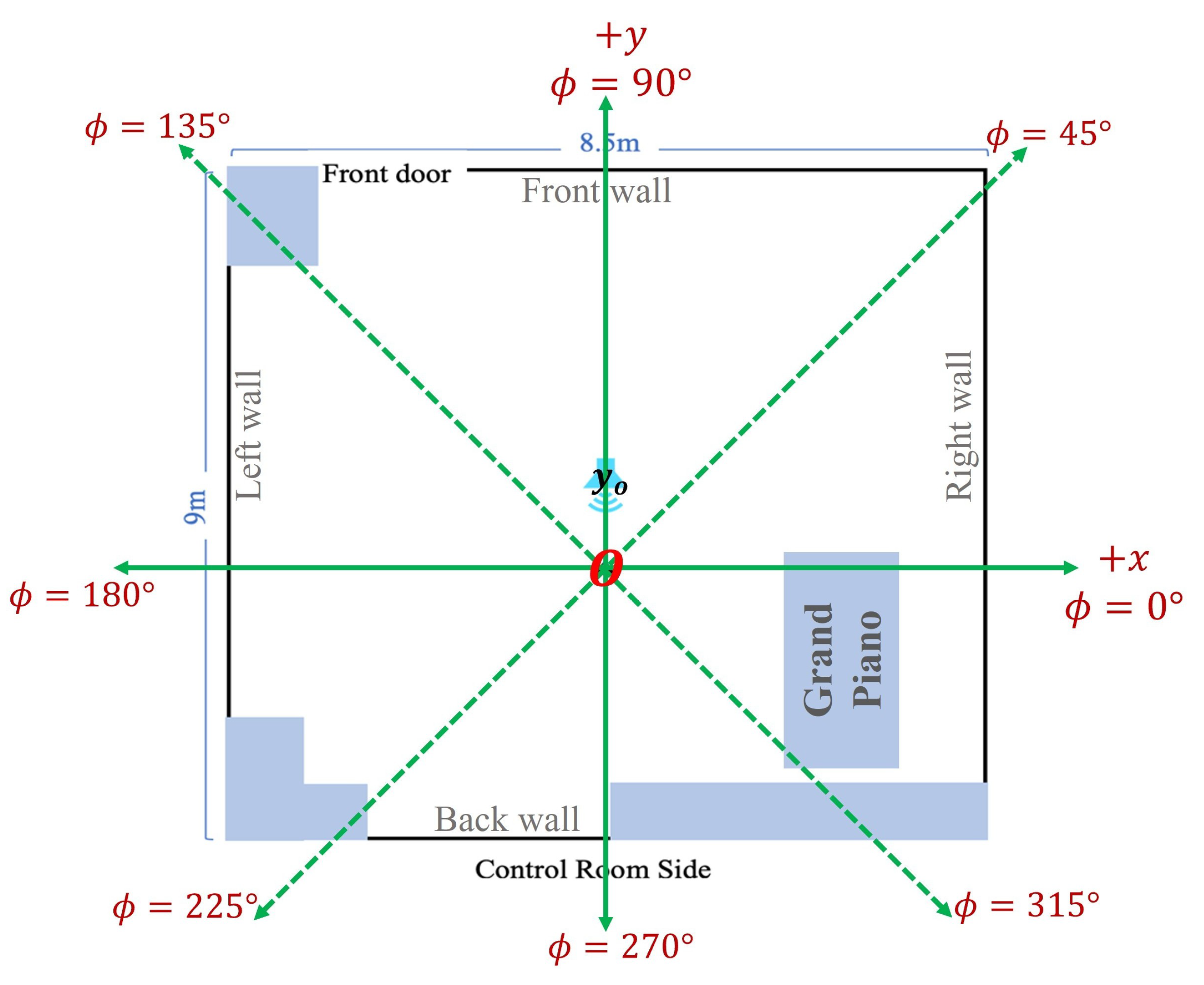
The rest of this paper is organized as follows. Section 2 outlines the methodology, reviewing the implementation of the eigenbeam–vMF-based analyzer. Section 3 provides the room description and experimental set-up, including the specific configurations of the recording studio. Section 4 describes the processing steps for the EM32 and NT-SF1 measurements, with array-specific parameters. Section 5 presents the results and discussion, comparing the acoustic features captured by both microphone arrays under different panel settings. Section 6 discusses the practical implications, limitations, and future directions of the proposed analysis. Finally, Section 7 concludes with a summary of the key findings, emphasizing the feasibility of first-order microphone arrays for practical room acoustic analysis.

2. Methodology: Eigenbeam–vMF-Based Room Acoustic Analyzer

The eigenbeam–vMF-based analyzer introduced in [25] enables time–frequency–direction-dependent characterization of room reflections. This section reviews its underlying framework and implementation, which involves two stages: estimation of the angular reflection power using the eigenbeam spatial correlation model and directivity modeling via vMF-based clustering to represent the anisotropic reflection features.

All notations and symbols used in this section are defined at their first occurrence in the text. The key variables and their physical meanings are summarized below:

• $\mathit{O}$	Coordinate origin or center of the microphone array;
• ${\mathit{y}}_o$	Position of the sound source;
• $\mathit{x}$	Position of the observation point (microphone);
• $k={\displaystyle \frac{2\pi f}{c}}$	Wavenumber, where f denotes the frequency in the time–frequency domain and c is the speed of sound;
• t	Temporal frame index in the time–frequency domain;
• $\mathbf{\Psi }(k,t,\mathit{x}|{\mathit{y}}_o)$	Observed sound pressure at $\mathit{x}$ in the time–frequency domain for a source located at ${\mathit{y}}_o$;
• ${\alpha }_{nm}(k,t|{\mathit{y}}_o)$	SH coefficients of the sound field, where $\{0\le n\le N\}$ is the order and $\{-n\le m\le n\}$ is the mode;
• ${\mathcal{P}}_D(k,t|{\mathit{y}}_o)$	Power of the direct sound;
• $\widehat{\mathit{y}}\equiv (\theta ,\varphi )$	Direction of incoming reflection with respect to $\mathit{O}$, where $\theta \in [0,\pi ]$ is the elevation angle and $\varphi \in [0,2\pi )$ is the azimuth angle;
• ${\mathcal{P}}_R(k,t,\widehat{\mathit{y}}|{\mathit{y}}_o)$	Power of the reflected sound field corresponding to the direction $\widehat{\mathit{y}}$;
• ${\Gamma }_{vu}(k,t|{\mathit{y}}_o)$	SH coefficients of ${\mathcal{P}}_R$, where $\{0\le v\le V\}$ is the order and $\{-v\le u\le v\}$ is the mode;
• ${\mathcal{P}}_T(k,t|{\mathit{y}}_o)$	Total reflection power at $\mathit{O}$, representing the time–frequency-dependent reflection power response;
• ${\left\{{\mathcal{P}}_R(k,t,\widehat{\mathit{y}}|{\mathit{y}}_o)\right\}}_{\widehat{\mathit{y}}}$	Set of ${\mathcal{P}}_R(k,t,\widehat{\mathit{y}}|{\mathit{y}}_o)$ samples over $\widehat{\mathit{y}}$;
• ${\mathbf{D}}_{k,t|{\mathit{y}}_o}$	Set of 3D unit vectors obtained by transforming ${\left\{{\mathcal{P}}_R(k,t,\widehat{\mathit{y}}|{\mathit{y}}_o)\right\}}_{\widehat{\mathit{y}}}$;
• $F\left(\mathfrak{X};{\mathbf{\Pi }}_{k,t|{\mathit{y}}_o}\right)$	vMF mixture model representing the directional density of ${\mathbf{D}}_{k,t|{\mathit{y}}_o}$, where $\mathfrak{X}$ is a 3D unit vector and ${\mathbf{\Pi }}_{k,t|{\mathit{y}}_o}=$ $\{{\mathsf{\mu }}_1,\cdots ,{\mathsf{\mu }}_{\mathcal{A}};$ ${\kappa }_1,\cdots ,{\kappa }_{\mathcal{A}};w_1,\cdots ,w_{\mathcal{A}}\}$ denotes the following model parameters:
	∘ ${\mathsf{\mu }}_a$	Mean direction of the ath vMF component;
	∘ ${\kappa }_a$	Concentration parameter controlling dispersion around ${\mathsf{\mu }}_a$;
	∘ $w_a$	Weight of the ath vMF component;
	∘ $\mathcal{A}$	Number of vMF components in the mixture.

2.1. Signal Model

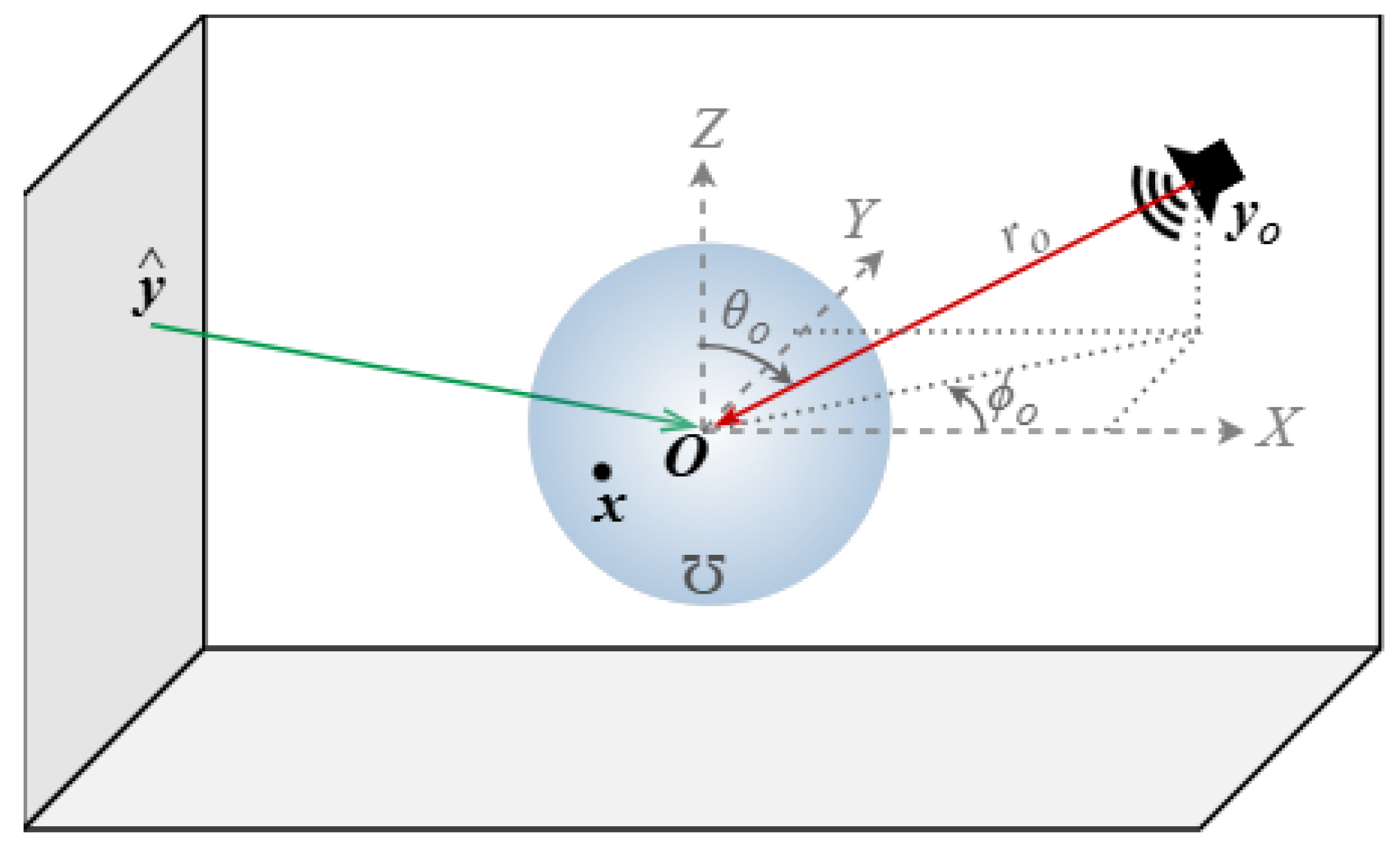
Consider an acoustic enclosure with a sound source located at ${\mathit{y}}_o\in {\mathbb{R}}^3$. To observe the resulting sound field, we define a source-free spherical region $\mho \subset {\mathbb{R}}^3$ centered at $\mathit{O}$. With $\mathit{O}$ as the coordinate origin, spatial points are expressed in spherical coordinates $(r,\theta ,\varphi )$, where $r\in [0,\infty )$ is the radial distance from $\mathit{O}$, $\theta \in [0,\pi ]$ is the elevation angle measured downward from the Z-axis, and $\varphi \in [0,2\pi )$ is the azimuth angle measured counterclockwise from the X-axis in the XY-plane. Following this convention, $(r_o,{\theta }_o,{\varphi }_o)$ denote the spherical coordinates of ${\mathit{y}}_o$, as shown in Figure 1.

Under the assumption of a linear time-invariant system, the sound pressure observed at a point $\mathit{x}\in \mho$ can be expressed as

$$\psi (\tau ,\mathit{x}|{\mathit{y}}_o)=s\left(\tau \right)\ast \underset{h(\tau ,\mathit{x},{\mathit{y}}_o)}{\underbrace{\left[h_{\mathrm{d}}(\tau ,\mathit{x},{\mathit{y}}_o)+h_{\mathrm{r}}(\tau ,\mathit{x},{\mathit{y}}_o)\right]}},$$

(1)

where $\tau$ denotes the discrete time index, $s\left(\tau \right)$ is the source excitation signal, $h(\tau ,\mathit{x},{\mathit{y}}_o)$ is the room impulse response (RIR) between ${\mathit{y}}_o$ and $\mathit{x}$, and ∗ denotes convolution. The RIR comprises $h_{\mathrm{d}}(·)$, corresponding to the direct sound, and $h_{\mathrm{r}}(·)$, corresponding to reflected components from the environment.

By applying short-time Fourier transform (STFT) to Equation (1), the sound pressure can be expressed in the time–frequency domain as follows:

$$\mathbf{\Psi }(k,t,\mathit{x}|{\mathit{y}}_o)=S(k,t)\left[H_{\mathrm{d}}(k,t,\mathit{x},{\mathit{y}}_o)+H_{\mathrm{r}}(k,t,\mathit{x},{\mathit{y}}_o)\right],$$

(2)

where $k=2\pi f/c$ is the wavenumber, with f and c denoting the frequency and speed of sound, respectively, and t is the temporal frame index. $S(k,t)$, $H_{\mathrm{d}}(k,t,\mathit{x},{\mathit{y}}_o)$, and $H_{\mathrm{r}}(k,t,\mathit{x},{\mathit{y}}_o)$ represent the STFTs of $s\left(\tau \right)$, $h_{\mathrm{d}}(\tau ,\mathit{x},{\mathit{y}}_o)$, and $h_{\mathrm{r}}(\tau ,\mathit{x},{\mathit{y}}_o)$, respectively.

In the spatial domain, $H_{\mathrm{d}}(k,t,\mathit{x},{\mathit{y}}_o)$ and $H_{\mathrm{r}}(k,t,\mathit{x},{\mathit{y}}_o)$ can be represented using a composition of plane waves as follows

$$\begin{array}{cc}\hfill H_{\mathrm{d}}(k,t,\mathit{x},{\mathit{y}}_o)& =G_{\mathrm{d}}(k,t|{\mathit{y}}_o)e^{ik{\widehat{\mathit{y}}}_o·\mathit{x}},\hfill \end{array}$$

(3a)

$$\begin{array}{cc}\hfill H_{\mathrm{r}}(k,t,\mathit{x},{\mathit{y}}_o)& ={\int }_{\widehat{\mathit{y}}}{G}_{\mathrm{r}}(k,t,\widehat{\mathit{y}}|{\mathit{y}}_o)e^{ik\widehat{\mathit{y}}·\mathit{x}}d\widehat{\mathit{y}},\hfill \end{array}$$

(3b)

where $G_{\mathrm{d}}(k,t|{\mathit{y}}_o)\in \mathbb{C}$ is the gain at $\mathit{O}$ associated with the direct sound arriving from direction ${\widehat{\mathit{y}}}_o\equiv ({\theta }_o,{\varphi }_o)$, $G_{\mathrm{r}}(k,t,\widehat{\mathit{y}}|{\mathit{y}}_o)\in \mathbb{C}$ is the gain at $\mathit{O}$ associated with the reflected sound arriving from direction $\widehat{\mathit{y}}\equiv (\theta ,\varphi )$, ${\int }_{\widehat{\mathit{y}}}d\widehat{\mathit{y}}={\int }_0^{2\pi }{\int }_0^{\pi }sin\theta d\theta d\varphi$, e is Euler’s number, and $i=\sqrt{-1}$. Substituting Equation (3) into Equation (2) yields

$$\mathbf{\Psi }(k,t,\mathit{x}|{\mathit{y}}_o)=S(k,t)G_{\mathrm{d}}(k,t|{\mathit{y}}_o)e^{ik{\widehat{\mathit{y}}}_o·\mathit{x}}+S(k,t){\int }_{\widehat{\mathit{y}}}{G}_{\mathrm{r}}(k,t,\widehat{\mathit{y}}|{\mathit{y}}_o)e^{ik\widehat{\mathit{y}}·\mathit{x}}d\widehat{\mathit{y}}.$$

(4)

Based on the second term on the right-hand side of Equation (4), the power of the reflected component arriving from direction $\widehat{\mathit{y}}$ can be expressed as follows:

$${\mathcal{P}}_R(k,t,\widehat{\mathit{y}}|{\mathit{y}}_o)=\mathbb{E}\left\{{\left|S\right(k,t\left)\right|}^2\right\}\mathbb{E}\left\{{\left|G_{\mathrm{r}}(k,t,\widehat{\mathit{y}}|{\mathit{y}}_o)\right|}^2\right\},$$

(5)

where $\mathbb{E}\{·\}$ and $|·|$ denote the statistical expectation operator and absolute value, respectively.

${\mathcal{P}}_R(k,t,\widehat{\mathit{y}}|{\mathit{y}}_o)\in \mathbb{R}$ is the time–frequency-dependent directional power of the reflected sound field, capturing the effects of the reflective and absorptive properties of the environment. Source-dependent factors such as the directivity and excitation signal content also influence this measure. Thus, to characterize and analyze the reflection distribution across the enclosure, we need to estimate ${\mathcal{P}}_R(k,t,\widehat{\mathit{y}}|{\mathit{y}}_o)$ from the observed sound field $\mathbf{\Psi }(k,t,\mathit{x}|{\mathit{y}}_o)$ after separating the direct path contribution.

2.2. Reflection Power Estimation Using Eigenbeam Spatial Correlation Model

The eigenbeam spatial correlation model enables efficient separation of the direct and reflected components from the observed sound field by exploiting an SH-domain relationship equivalent to Equation (4). For this purpose, the spherical function ${\mathcal{P}}_R(k,t,\widehat{\mathit{y}}|{\mathit{y}}_o)$ is decomposed using SH-basis functions as follows:

$${\mathcal{P}}_R(k,t,\widehat{\mathit{y}}|{\mathit{y}}_o)=\Re \left(\sum _{v=0}^{\infty }\sum _{u=-v}^v{\Gamma }_{vu}(k,t|{\mathit{y}}_o)Y_{vu}\left(\widehat{\mathit{y}}\right)\right),$$

(6)

where ${\Gamma }_{vu}(k,t|{\mathit{y}}_o)$ are the reflection power coefficients, $Y_{vu}(·)$ is the SH function of the vth order and uth mode, and $\Re (·)$ denotes the real component of a complex argument.

The sound pressure $\mathbf{\Psi }(k,t,\mathit{x}|{\mathit{y}}_o)$ can also be represented in the SH domain following the solution of Helmholtz wave equation for an interior sound field as follows [30]:

$$\mathbf{\Psi }(k,t,\mathit{x}|{\mathit{y}}_o)=\sum _{n=0}^{\infty }\sum _{m=-n}^n{\alpha }_{nm}(k,t|{\mathit{y}}_o)j_n\left(k\parallel \mathit{x}\parallel \right)Y_{nm}\left(\widehat{\mathit{x}}\right),$$

(7)

where ${\alpha }_{nm}(k,t|{\mathit{y}}_o)$ are the SH coefficients of the spatial sound field, also known as eigenbeams or frequency-domain ambisonic signals, $j_n(·)$ is the nth-order spherical Bessel function of the first kind, and $\parallel \mathit{x}\parallel$ and $\widehat{\mathit{x}}$ are the Euclidean norm and direction of $\mathit{x}$, respectively. The correlation of the ${\alpha }_{nm}$ coefficients relates to the reflection coefficients ${\Gamma }_{vu}$ as follows:

$$\begin{array}{cc}\hfill \mathbb{E}\{{\alpha }_{nm}(k,t|{\mathit{y}}_o)& {\alpha }_{n^{\prime }{m}^{\prime }}^{*}(k,t|{\mathit{y}}_o)\}=C_{n{n}^{\prime }}[{\mathcal{P}}_D(k,t|{\mathit{y}}_o)Y_{nm}^{*}\left({\widehat{\mathit{y}}}_o\right)Y_{n^{\prime }{m}^{\prime }}\left({\widehat{\mathit{y}}}_o\right)\hfill \\ \hfill & +{(-1)}^m\sum _{v=0}^{\infty }\sum _{u=-v}^v{\Gamma }_{vu}(k,t|{\mathit{y}}_o)\sqrt{{\displaystyle \frac{(2v+1)(2n+1)(2n^{\prime }+1)}{4\pi }}}{W}_1{W}_2],\hfill \end{array}$$

(8)

where $C_{n{n}^{\prime }}=16{\pi }^2{i}^{(n-n^{\prime })}$, ${\mathcal{P}}_D(k,t|{\mathit{y}}_o)=\mathbb{E}\left\{{\left|S\right(k,t\left)\right|}^2\right\}\mathbb{E}\left\{{\left|G_{\mathrm{d}}(k,t|{\mathit{y}}_o)\right|}^2\right\}$ is the direct path power, ${(·)}^{*}$ denotes complex conjugation, and $W_1$ and $W_2$ are the Wigner 3j symbols [31] given by $W_1=\left(\begin{array}{ccc}v& n& n^{\prime }\\ 0& 0& 0\end{array}\right)$ and $W_2=\left(\begin{array}{ccc}v& n& n^{\prime }\\ u& -m& m^{\prime }\end{array}\right)$. For the detailed derivation of Equation (8), please refer to Chapter 3 of [32].

From $\mathbf{\Psi }(k,t,\mathit{x}|{\mathit{y}}_o)$, measured at different positions $\mathit{x}$ using any microphone array, we can estimate ${\alpha }_{nm}(k,t|{\mathit{y}}_o)$ for $\{n\in \mathbb{W}\mid 0\le n\le N\}$ and $\{m\in \mathbb{Z}\mid -n\le m\le n\}$ by applying array-dependent processing techniques [10,11,26,33,34,35,36,37,38]. The maximum limit of N is restricted by the number of microphones to avoid spatial aliasing [10]. Using ${\alpha }_{nm}\forall (n,m)$, Equation (8) can be transformed into a matrix equation:

$$\underset{\mathbf{\Lambda }(k,t|{\mathit{y}}_o)}{\underbrace{\left[\begin{array}{c}{\Lambda }_{0000}\\ {\Lambda }_{001–1}\\ ⋮\\ {\Lambda }_{00NN}\\ {\Lambda }_{1–100}\\ ⋮\\ {\Lambda }_{NNNN}\end{array}\right]}}=\underset{\mathit{B}\left(k\right|{\mathit{y}}_o)}{\underbrace{\left[\begin{array}{cccc}{\rho }_{0000}& {\sigma }_{000000}& \cdots & {\sigma }_{0000VV}\\ {\rho }_{001–1}& {\sigma }_{001–100}& \cdots & {\sigma }_{001–1VV}\\ ⋮& ⋮& ⋮& ⋮\\ {\rho }_{00NN}& {\sigma }_{00NN00}& \cdots & {\sigma }_{00NNVV}\\ {\rho }_{1–100}& {\sigma }_{1–10000}& \cdots & {\sigma }_{1–100VV}\\ ⋮& ⋮& ⋮& ⋮\\ {\rho }_{NNNN}& {\sigma }_{NNNN00}& \cdots & {\sigma }_{NNNNVV}\end{array}\right]}}\underset{\mathbf{\Omega }(k,t|{\mathit{y}}_o)}{\underbrace{\left[\begin{array}{c}{\mathcal{P}}_D\\ {\Gamma }_{00}\\ {\Gamma }_{1–1}\\ ⋮\\ {\Gamma }_{V–V}\\ ⋮\\ {\Gamma }_{VV}\end{array}\right]}},$$

(9)

where $\mathbf{\Lambda }(k,t|{\mathit{y}}_o)$ is a column vector of a size $[{(N+1)}^4\times 1]$ with

$${\Lambda }_{nm{n}^{\prime }{m}^{\prime }}=\mathbb{E}\left\{{\alpha }_{nm}(k,t|{\mathit{y}}_o){\alpha }_{n^{\prime }{m}^{\prime }}^{*}(k,t|{\mathit{y}}_o)\right\},$$

(10)

$\mathit{B}\left(k\right|{\mathit{y}}_o)$ is a matrix of a size $[{(N+1)}^4\times ({(V+1)}^2+1)]$ with elements

$${\rho }_{nm{n}^{\prime }{m}^{\prime }}=C_{n{n}^{\prime }}{Y}_{nm}^{*}\left({\widehat{\mathit{y}}}_o\right)Y_{n^{\prime }{m}^{\prime }}\left({\widehat{\mathit{y}}}_o\right),$$

(11)

$${\sigma }_{nm{n}^{\prime }{m}^{\prime }vu}={(-1)}^m{C}_{n{n}^{\prime }}\sqrt{{\displaystyle \frac{(2v+1)(2n+1)(2n^{\prime }+1)}{4\pi }}}{W}_1{W}_2,$$

(12)

and $\mathbf{\Omega }(k,t|{\mathit{y}}_o)$ is a column vector of a size $[({(V+1)}^2+1)\times 1]$.

We can construct elements of $\mathbf{\Lambda }(k,t|{\mathit{y}}_o)$ from the ${\alpha }_{nm}(k,t|{\mathit{y}}_o)$ coefficients and form $\mathit{B}\left(k\right|{\mathit{y}}_o)$ from known functions. The unknown $\mathbf{\Omega }(k,t|{\mathit{y}}_o)$ can then be estimated by solving Equation (9) using the least squares method given by

$$\widehat{\mathbf{\Omega }}(k,t|{\mathit{y}}_o)={\mathit{B}}^{†}\left(k\right|{\mathit{y}}_o)\mathbf{\Lambda }(k,t|{\mathit{y}}_o),$$

(13)

where $\widehat{[·]}$ and ${[·]}^{†}$ denote the estimated value and the Moore–Penrose pseudo-inverse, respectively, computed using singular value decomposition. While solving Equation (13), the maximum admissible order of ${\Gamma }_{vu}$ is limited to $V_{\max }=⌊\sqrt{{(N+1)}^4-1}-1⌋$, ensuring that the system is not under-determined. In practice, V is selected within this bound by considering the conditioning of $\mathit{B}\left(k\right|{\mathit{y}}_o)$ to avoid numerically unstable solutions.

We can now extract ${\Gamma }_{vu}(k,t|{\mathit{y}}_o)$ from $\widehat{\mathbf{\Omega }}$ and then substitute in Equation (6), truncated to V, to compute ${\mathcal{P}}_R(k,t,\widehat{\mathit{y}}|{\mathit{y}}_o)$ for different $\widehat{\mathit{y}}$ directions. By analyzing the temporal response of ${\mathcal{P}}_R(k,t,\widehat{\mathit{y}}|{\mathit{y}}_o)$, we can directly estimate the directional decay time for each $\widehat{\mathit{y}}$.

In addition, by applying the SH symmetrical property [30] to Equation (6), we can obtain the total reflection power received at $\mathit{O}$ as follows:

$${\mathcal{P}}_T(k,t|{\mathit{y}}_o)={\int }_{\widehat{\mathit{y}}}{\mathcal{P}}_R(k,t,\widehat{\mathit{y}}|{\mathit{y}}_o)d\widehat{\mathit{y}}=\sqrt{4\pi }{\Gamma }_{00}(k,t|{\mathit{y}}_o).$$

(14)

This quantity represents the time–frequency-dependent reflection power response.

2.3. Reflection Directivity Modeling

Let ${\left\{{\mathcal{P}}_R(k,t,\widehat{\mathit{y}}|{\mathit{y}}_o)\right\}}_{\widehat{\mathit{y}}}$ be a dataset of ${\mathcal{P}}_R(k,t,\widehat{\mathit{y}}|{\mathit{y}}_o)$ over sufficiently sampled $\widehat{\mathit{y}}$ directions in a 3D space. This dataset encompasses both anisotropic (non-diffuse) and isotropic (nearly diffuse) reflection fields, with their relative contributions varying based on the nature of the room, sound frequency, and decay factors [18,39]. Early reflections primarily exhibit anisotropic distribution governed by the source location, while late reflections tend to become isotropic due to increased scattering. The presence of dominant room modes in low frequencies can also contribute to anisotropic features. To understand these directional variations, we convert ${\left\{{\mathcal{P}}_R(k,t,\widehat{\mathit{y}}|{\mathit{y}}_o)\right\}}_{\widehat{\mathit{y}}}$ into a more interpretable form by fitting a statistical directional density model.

The most suitable model capable of representing such multi-modal data using the minimum parameters is a convex mixture of vMF distributions [40] given by

$$F\left(\mathfrak{X};{\mathbf{\Pi }}_{k,t|{\mathit{y}}_o}\right)=\sum _{a=1}^{\mathcal{A}}{w}_a\underset{f_{\mathrm{vMF}}}{\underbrace{{\displaystyle \frac{\sqrt{{\kappa }_a}}{{\left(2\pi \right)}^{\frac{3}{2}}{I}_{\left(\frac{1}{2}\right)}\left({\kappa }_a\right)}}exp\left({\kappa }_a{\mathsf{\mu }}_a^T\mathfrak{X}\right)}},$$

(15)

where $\mathfrak{X}\in {\mathbb{R}}^3$ is a point on the surface of a unit sphere (i.e., a 3D unit vector with $\parallel \mathfrak{X}\parallel =1$), $f_{\mathrm{vMF}}$ is the 3D vMF probability density function characterized by the mean direction vector ${\mathsf{\mu }}_a$ $\left(\parallel {\mathsf{\mu }}_a\parallel =1\right)$ and the concentration parameter ${\kappa }_a$ $\left({\kappa }_a\ge 0\right)$, $I_{\nu }(·)$ is the modified Bessel function of the first kind at order $\nu$, and $F(·)$ is the compound model composed of $\mathcal{A}$ distinct $f_{\mathrm{vMF}}$ mixed in proportion to the convex weights $w_a$. The parameters of component $f_{\mathrm{vMF}}$ constitute the compound model parameter ${\mathbf{\Pi }}_{k,t|{\mathit{y}}_o}=\left\{{\mathsf{\mu }}_1,\cdots ,{\mathsf{\mu }}_{\mathcal{A}};{\kappa }_1,\cdots ,{\kappa }_{\mathcal{A}};w_1,\cdots ,w_{\mathcal{A}}\right\}$.

For our data, the ${\mathsf{\mu }}_a$ parameters would imply dominant reflection directions, ${\kappa }_a$ quantifies the dispersion of reflected power distribution from ${\mathsf{\mu }}_a$, $w_a$ decides the relative strength of each ${\mathsf{\mu }}_a$, and $\mathcal{A}$ indicates the number of dominant reflection directions. The range of $\mathcal{A}$ will be limited for a given room based on the presence of distinct reflective surfaces. We can, therefore, analyze the sought reflection features with the knowledge of ${\mathbf{\Pi }}_{k,t|{\mathit{y}}_o}$.

According to the definition in Equation (15), ${\left\{{\mathcal{P}}_R(k,t,\widehat{\mathit{y}}|{\mathit{y}}_o)\right\}}_{\widehat{\mathit{y}}}$ should be transformed to samples on a unit sphere prior to fitting the vMF model. We generate this transformed data, ${\mathbf{D}}_{k,t|{\mathit{y}}_o}$, as a composition of 3D direction vectors such that their distribution expresses the relative magnitude of angular reflection power across the 3D space; in other words, if $\overrightarrow{\mathit{y}}=\left(sin\theta cos\varphi ,sin\theta sin\varphi ,cos\theta \right)$ is the 3D Cartesian unit vector corresponding to the $\widehat{\mathit{y}}$ direction, then the statistical frequency (repetitions) of $\overrightarrow{\mathit{y}}$ in ${\mathbf{D}}_{k,t|{\mathit{y}}_o}$ is set to be proportional to $\left|{\mathcal{P}}_R(k,t,\widehat{\mathit{y}}|{\mathit{y}}_o)\right|$. Finally, we perform vMF-mixture model fitting on ${\mathbf{D}}_{k,t|{\mathit{y}}_o}$ to estimate ${\mathbf{\Pi }}_{k,t|{\mathit{y}}_o}$ by employing an expectation-maximization (EM) algorithm [41] integrated with clustering based on the Bayesian minimum message length criterion [42]. This criterion automatically determines the optimal value for $\mathcal{A}$ that would best fit the input data, while allowing an upper bound to be specified to control model complexity.

By substituting the estimated ${\mathbf{\Pi }}_{k,t|{\mathit{y}}_o}$ into Equation (15), we can generate the reflection directivity model $F\left(\mathfrak{X};{\mathbf{\Pi }}_{k,t|{\mathit{y}}_o}\right)$ and scale it with ${\mathcal{P}}_T(k,t|{\mathit{y}}_o)$ to assimilate the time–frequency response of the reflection power. Examining scaled F allows analysis of the directional characteristics of the reflected sound field across time and frequency.

Additionally, we examine the directivity time-span parameter introduced in [25]. This parameter indicates the lifespan of the anisotropic reflection field before it decays into a weak diffused field. It is measured for each frequency as the time duration for which vector clusters are identifiable in ${\mathbf{D}}_{k,t|{\mathit{y}}_o}$, i.e., when ${\mathbf{\Pi }}_{k,t|{\mathit{y}}_o}$ is determinable.

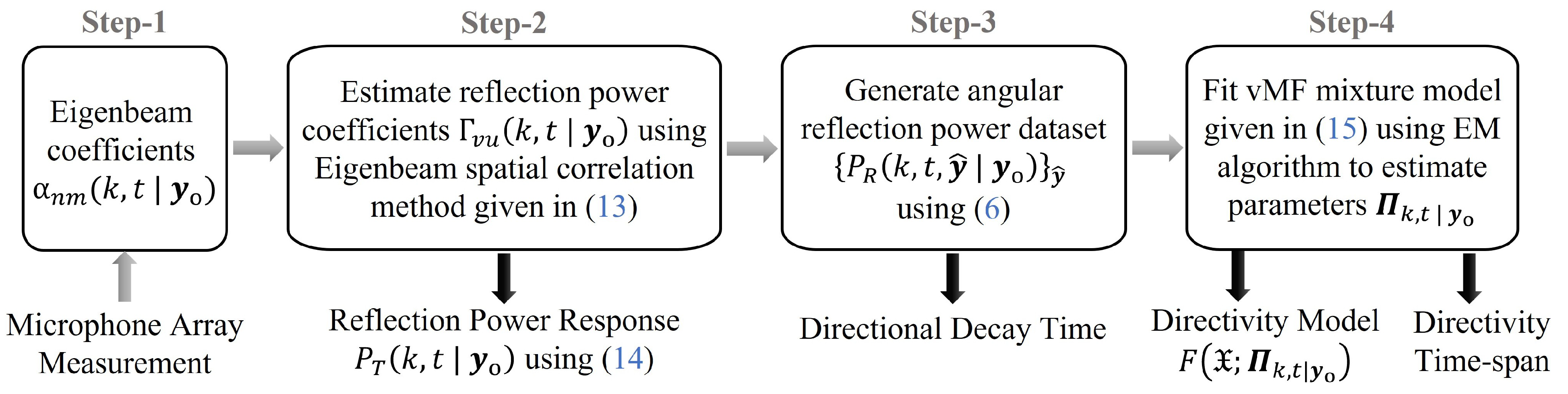
The overall implementation pipeline of the eigenbeam–vMF-based analyzer, as described in Section 2.1, Section 2.2 and Section 2.3, is summarized in Figure 2. From a microphone array measurement, the analyzer enables multifaceted characterization of the reflected sound field through a set of derived quantities. The maximum SH order and fidelity of ${\alpha }_{nm}$ coefficients in Step 1 depend on the array specifications and consequently constrain the detail captured in these quantities.

3. Test Environment and Analysis Set-Up

To compare the effectiveness of first-order and higher-order microphone arrays for room acoustic characterization using the eigenbeam–vMF-based analyzer, we considered a recording studio at the Australian National University (ANU) [43] as the test environment. The analysis is performed using RIRs of this room obtained from the RSoANU dataset [44]. The following subsections describe the room environment and the measurement set-up considered in this study, including the microphone arrays under comparison.

3.1. Room Description and Configurations

The recording studio features floor dimensions of 8.5 m × 9 m and a double-height space with a floor-to-ceiling height of 5.6 m. Two adjacent walls are fitted with variable wall paneling, offering options in both wood and felt materials, while the other two walls have fixed paneling. The structural details of the wooden and felt panels are mentioned in [45]. The room also includes a window and a sliding door made of glass material, providing access to the control room. Various furniture and musical instruments, particularly a grand piano, also occupy the room.

We considered two environmental configurations: all variable panels set to wood or felt, as shown in Figure 3a and Figure 3b, respectively. The arrangement of all other objects in the room remained unchanged across the two configurations. The wood and felt configurations yielded an average $T_{20}$ of 0.84 s and 0.74 s, respectively.

3.2. Measurement Devices

The RSoANU dataset employed a Tannoy System 600 loudspeaker (Tannoy Ltd., Coatbridge, UK) as the sound source and recorded RIRs using two microphone arrays: a Rode NT-SF1 (RØDE Microphones, Sydney, Australia) and an mh acoustics EM32 Eigenmike (mh acoustics LLC, Summit, NJ, USA). Photographs of the loudspeaker and microphone arrays are shown in Figure 4.

The NT-SF1 comprises four matched cardioid condenser microphone capsules arranged in a tetrahedral array, capable of capturing spatial sound in first-order ambisonics [46]. The EM32 consists of 32 omnidirectional electret microphones mounted on a rigid sphere of $4.2$-cm radius, capable of capturing up to fourth-order ambisonics [47]. The important specifications of these microphone arrays are summarized in

Table 1. Comparison of microphone arrays: Rode NT-SF1 and EM32 Eigenmike [46,47].

	Rode NT-SF1	EM32 Eigenmike
Number of microphones	4	32
Microphone type	12.7 mm true-condenser	14 mm electret
Microphone polar pattern	Cardioid	Omnidirectional
Array geometry	Tetrahedral	Rigid sphere
Array radius	∼2.3 cm	4.2 cm
Maximum ambisonic order	1	4
SH degrees of freedom	4	25
Frequency response $(\pm 3\mathrm{dB})$	30 Hz–20 kHz	30 Hz–20 kHz
Approximate cost (USD)	∼1000–1500	∼15,000–20,000
Weight	286 g	500 g

. Based on the ambisonic order (N) and array radius (R), the theoretical upper frequency limit before spatial aliasing can be approximated with $f_{\mathrm{alias}}\approx {\displaystyle \frac{cN}{2\pi R}}$. This limit is ∼2.4 kHz for the NT-SF1 and ∼5.2 kHz for the EM32, which influences their ability to resolve the directional features of reflections at high frequencies. The EM32 supports a wider usable spatial frequency range and improved spatial sampling compared with the NT-SF1 but at a significantly higher cost.

3.3. Measurement Geometry

The layout of the acoustic setting considered for analysis is shown in Figure 5. The variable wall panels were positioned along the front and right walls. The microphone array was centered at $\mathit{O}=[4.25,3.75,1.7]$ m, and the loudspeaker was placed at ${\mathit{y}}_o=[4.25,4.75,1.514]$ m, with both relative to the room’s bottom-left corner. We consider $\mathit{O}$ as the coordinate origin and hence ${\mathit{y}}_o=(1.0172\mathrm{m},{101}^{\circ },{90}^{\circ })$ relative to $\mathit{O}$. The loudspeaker is directional, as evident from Figure 4a, and it was positioned to face the control room, as depicted in Figure 5.

For this set-up, we examine the acoustic characteristics under the wood and felt panel configurations, with emphasis on comparing the performance of the NT-SF1 and EM32 microphone arrays using the eigenbeam–vMF-based analyzer.

4. Measurement Processing

Here, we specify the processing of the EM32 and NT-SF1 microphone array measurements following the implementation steps shown in Figure 2. From the RSoANU dataset [44], we chose the RIRs recorded by these microphone arrays corresponding to the source–receiver locations depicted in Figure 5.

The RIRs, sampled at 48 kHz, were convolved with a white Gaussian noise (WGN) signal of $0.1$ s duration to generate microphone recordings for both EM32 and NT-SF1. By applying STFT using a 1024-sample Hanning window with $50\%$ overlap and a 2048-point fast Fourier transform, these recordings were converted into the time–frequency domain.

From the 32-channel EM32 recording, the corresponding eigenbeam coefficients ${\alpha }_{nm}^{\left(\mathrm{EM}32\right)}(k,t|{\mathit{y}}_o)$ were obtained by solving

$${\alpha }_{nm}^{\left(\mathrm{EM}32\right)}(k,t|{\mathit{y}}_o)={\displaystyle \frac{{\sum }_{q=1}^Q\mathbf{\Psi }(k,t,{\mathit{x}}_q|{\mathit{y}}_o)Y_{nm}^{*}\left({\widehat{\mathit{x}}}_q\right)}{b_n\left(kR\right)}}$$

(16)

using a least squares approach [10,48], where $R=4.2$ cm is the array radius, ${\mathit{x}}_q$ denotes the location of the qth microphone, for $q=1,2,\dots ,Q=32$, and

$$b_n\left(kR\right)=j_n\left(kR\right)-{\displaystyle \frac{j_n^{\prime }\left(kR\right)}{h_n^{\prime }\left(kR\right)}}{h}_n\left(kR\right)$$

(17)

is the mode strength. In Equation (17), $h_n(·)$ is the nth-order spherical Hankel function of the first kind, and ${(·)}^{\prime }$ indicates the first-order derivative operation. While solving Equation (16), the order of ${\alpha }_{nm}^{\left(\mathrm{EM}32\right)}$ was set to $N^{\left(\mathrm{EM}32\right)}\left(k\right)=\lceil keR/2\rceil$, with a maximum limit of 4, to mitigate errors arising from the high-pass behavior of higher-order Bessel functions and spatial aliasing.

In the RSoANU dataset, NT-SF1 RIRs were provided in Ambisonics B format, consisting of four channels $\{W,X,Y,Z\}$, where W is the omnidirectional component and $\{X,Y,Z\}$ are the directional components that correspond to the front-back, left-right, and up-down axes, respectively [26,46]. Let $\overline{W}$, $\overline{X}$, $\overline{Y}$, and $\overline{Z}$ denote the STFT of the corresponding WGN-convolved recordings. Based on the relation between real and complex forms of spherical harmonic solutions to the wave equation [49,50], we converted $\{\overline{W},\overline{X},\overline{Y},\overline{Z}\}$ into corresponding eigenbeam coefficients ${\alpha }_{nm}^{\left(\mathit{NT-SF}1\right)}(k,t|{\mathit{y}}_o)$ of order $N^{\left(\mathit{NT-SF}1\right)}\left(k\right)=1$ as follows:

$$\left[\begin{array}{c}{\alpha }_{00}^{\left(\mathit{NT-SF}1\right)}\\ {\alpha }_{1–1}^{\left(\mathit{NT-SF}1\right)}\\ {\alpha }_{10}^{\left(\mathit{NT-SF}1\right)}\\ {\alpha }_{11}^{\left(\mathit{NT-SF}1\right)}\end{array}\right]=\left[\begin{array}{cccc}1& 0& 0& 0\\ 0& -1/\sqrt{2}& i/\sqrt{2}& 0\\ 0& 0& 0& 1\\ 0& 1/\sqrt{2}& i/\sqrt{2}& 0\end{array}\right]\left[\begin{array}{c}\overline{W}\\ \overline{X}\\ \overline{Y}\\ \overline{Z}\end{array}\right].$$

(18)

From the derived eigenbeam coefficients of the EM32 and NT-SF1, Step 2 estimates the ${\Gamma }_{vu}(k,t|{\mathit{y}}_o)$ coefficients using Equation (13) over the frequency range of interest from 50 Hz to 5000 Hz. The corresponding frequency-dependent orders, given in

Table 2. Frequency-dependent values of N (order of ${\alpha }_{nm}$) and V (order of ${\Gamma }_{vu}$) used for the analyzer implementation with the two microphone arrays.

Microphone Array	Frequency Range (Hz)	N	V
EM32	50–960	1	2
	980–1920	2	3
	1945–2882	3	5
	2906–5000	4	7
NT-SF1	50–5000	1	2

, were selected in accordance with the admissible limits and conditioning considerations described in Section 2.2.

Subsequent steps were implemented with processing parameters chosen to balance spatial resolution and computational cost. In Step 3, ${\left\{{\mathcal{P}}_R(k,t,\widehat{\mathit{y}}|{\mathit{y}}_o)\right\}}_{\widehat{\mathit{y}}}$ was generated for 500 $\widehat{\mathit{y}}$ directions uniformly distributed in a spiral pattern on the 3D sphere [51]. For generating the vMF models $F\left(\mathfrak{X};{\mathbf{\Pi }}_{k,t|{\mathit{y}}_o}\right)$ in Step 4, $\mathfrak{X}$ was set to the unit sphere surface points sampled at a $2^{\circ }$ azimuth and elevation resolution.

5. Results and Discussion

This section analyzes the acoustic characteristics of the recording studio in both the wood and felt environments by examining (1) the spectral response of the reflection power, (2) dominant reflection directions, (3) directivity time-span, and (4) directional decay time, based on measurements from both the EM32 and the NT-SF1. Given the NT-SF1’s comparatively lower spatial resolution, we do not expect it to capture finer details as accurately as the EM32, but we aim to test its feasibility in analyzing essential acoustic features.

5.1. Spectral Response of Reflection Power

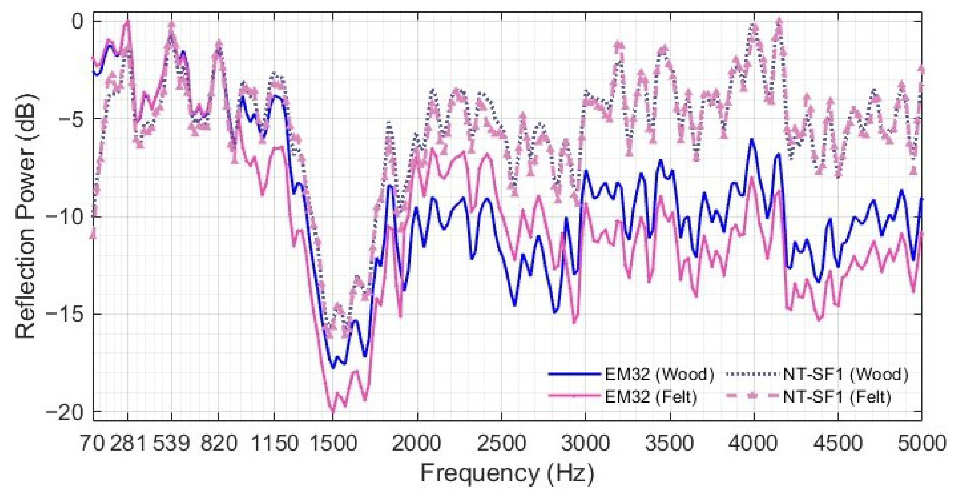
The spectral response of the total reflection power received at $\mathit{O}$, computed from time-averaged ${\mathcal{P}}_T(k,t|{\mathit{y}}_o)$, is shown in Figure 6. The responses between the EM32 and NT-SF1 closely overlap in the range of 200–900 Hz, where both arrays operate with first-order eigenbeams (refer to Table 2), suggesting that first-order measurements are sufficient to capture the reflection power response in the low-frequency range. Outside of this range, the EM32 and NT-SF1 exhibit magnitude differences, which become more pronounced beyond the spatial aliasing limit of the NT-SF1 (∼2.4 kHz; see Section 3.2). Since both microphones have relatively flat frequency responses (see Table 1) within the analysis range, these deviations are primarily attributed to array-dependent spatial sampling limitations. The equalization applied during RIR measurements may have also influenced these magnitude differences. Despite this, both microphone arrays show consistent trends, with coinciding peak and trough frequencies across the spectrum in both the felt and wood environments, indicating that the underlying spectral characteristics of the reflection field are reliably captured.

Prominent spectral peaks are visible at $\{281,539,820\}$ Hz in both the EM32 and NT-SF1 responses for both room environments, suggesting room-induced effects such as modal reinforcement or strong constructive interference. Based on the room volume and reverberation time, individual room modes are ideally expected to lose prominence above ≈90 Hz, as per the Schroeder frequency limit [52]. However, irregular wall structures and non-uniform surface materials of the actual room (Figure 3) likely contributed to interference patterns and spectral peaks beyond this threshold.

For the EM32, the felt environment clearly shows a lower magnitude than the wood in the ranges of 0.9–1.9 kHz and 2.8–5.0 kHz, which is expected due to the higher absorption property of felt material. The average reflection power is approximately $-7.4$ dB for wood and $-7.8$ dB for felt. However, the NT-SF1 exhibits only marginal differences between the two configurations, with averages of around $-4.7$ dB for wood and $-4.8$ dB for felt.

While both arrays perform similarly in the first-order regime (<0.9 kHz), the NT-SF1’s sparse sampling (four microphones) and first-order encoding ($N=1$) limit its spatial degrees of freedom and thereby its ability to resolve finer direction-dependent variations in reflection energy at higher frequencies. This leads to spatial smoothing and reduced sensitivity to the panel configurations. In comparison, the EM32, with denser sampling (32 microphones), higher-order representation (up to $N=4$), and an extended spatial bandwidth (∼5.2 kHz), retains these variations, enabling clearer discrimination between the configurations.

Note that the dip around $1.5$ kHz is caused by the loudspeaker response and is not a contribution from the room. The otherwise flat response of the loudspeaker between 52 Hz and 20 kHz [53] makes source coloration an unlikely cause of the observed peaks.

5.2. Dominant Reflection Directions

In the analysis of dominant reflection directions, we found that early reflections were primarily concentrated at lower elevations ($\theta >{90}^{\circ }$) for both the wood and felt settings. For ease of comparison, we examine the results across the azimuth directions only.

5.2.1. Wood Panel Configuration

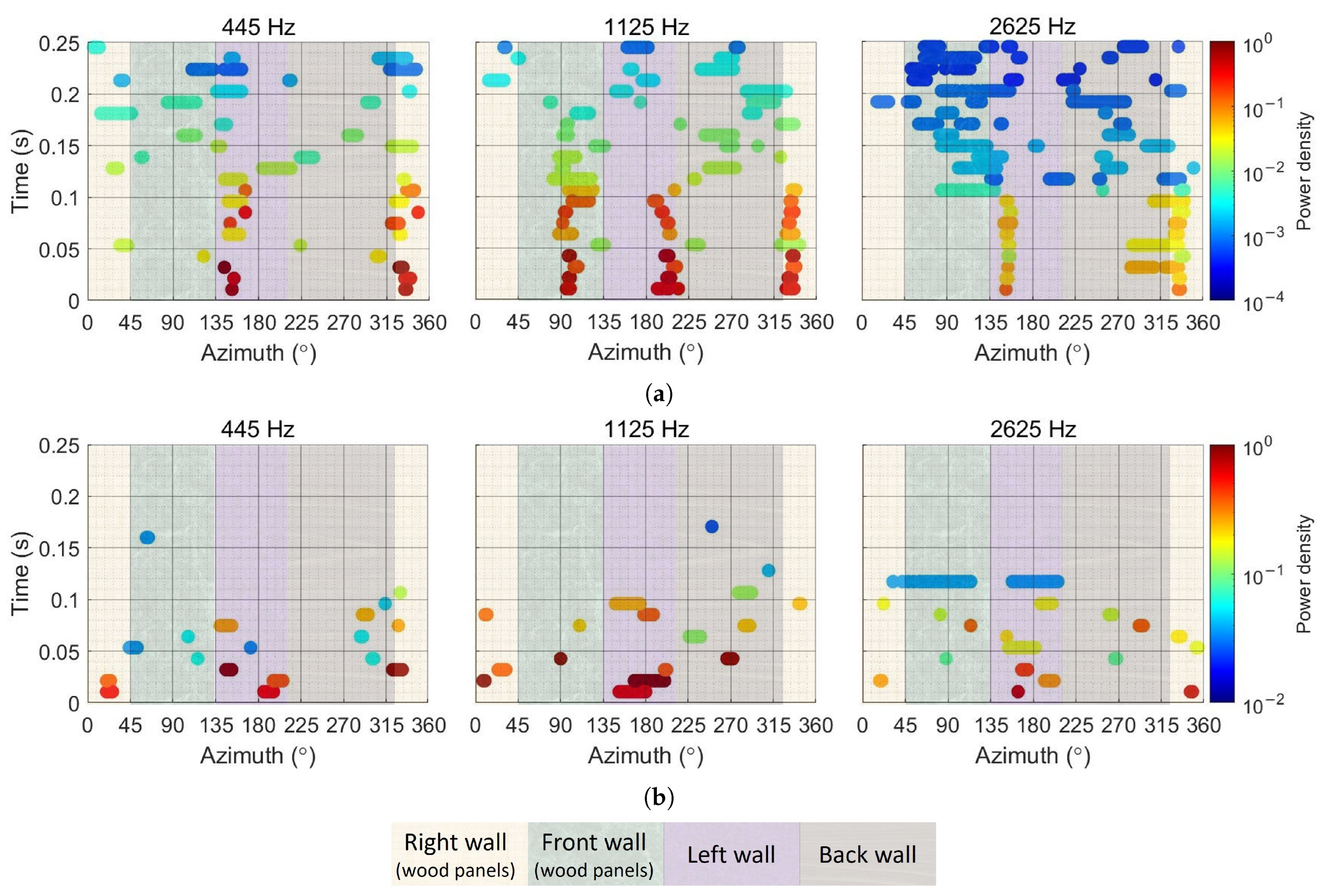
For the wood panel setting, the local azimuth maxima of the reflection directivity models $F\left(\mathfrak{X};{\mathbf{\Pi }}_{k,t|{\mathit{y}}_o}\right)$ over time for some selected frequencies based on the EM32 and NT-SF1 measurements are shown in Figure 7a and Figure 7b, respectively. In the EM32 results, we observe concentrated reflections around ≈150° on the left wall and around the back-right wall corner (≈330°) at 445 Hz and 2625 Hz during the active source period (≤0.1 s). At 1125 Hz, dominant reflections occur around ${90}^{\circ }$ (front wall), ${200}^{\circ }$ (back-left wall corner), and ${330}^{\circ }$ (back-right wall corner). For all three frequencies, a high power density around ${330}^{\circ }$ also coincides with the location of the grand piano (Figure 5), conforming with its highly reflective body (Figure 3). After the source ceases ($>0.1$ s), the local maxima become increasingly random over time, indicating a transition from a few dominant, spatially separable early reflections to a more complex, overlapping diffuse field. At these later time instants, the patterns appear more dispersed at higher frequencies due to increased wave scattering [54,55].

The pattern in the initial time instants of the NT-SF1 results in Figure 7b is not as recurring as that of the EM32 results. Moreover, we cannot observe the $F\left(\mathfrak{X};{\mathbf{\Pi }}_{k,t|{\mathit{y}}_o}\right)$ models for many time instants after 0.1 s, since the directional anisotropy of the decaying reflection field becomes obscured from detection with the NT-SF1’s limited spatial resolution. Nevertheless, the highest power densities (brown dots) observed around $\{{150}^{\circ }$, ${330}^{\circ }\}$ at 445 Hz, $\{{90}^{\circ }$, ${180}^{\circ }\}$ at 1125 Hz, and $\{{160}^{\circ }$, ${340}^{\circ }\}$ at 2625 Hz, agree with the EM32 results. Apart from the dominant directions, some secondary peaks also concur between Figure 7a,b, especially at 445 Hz.

5.2.2. Felt Panel Configuration

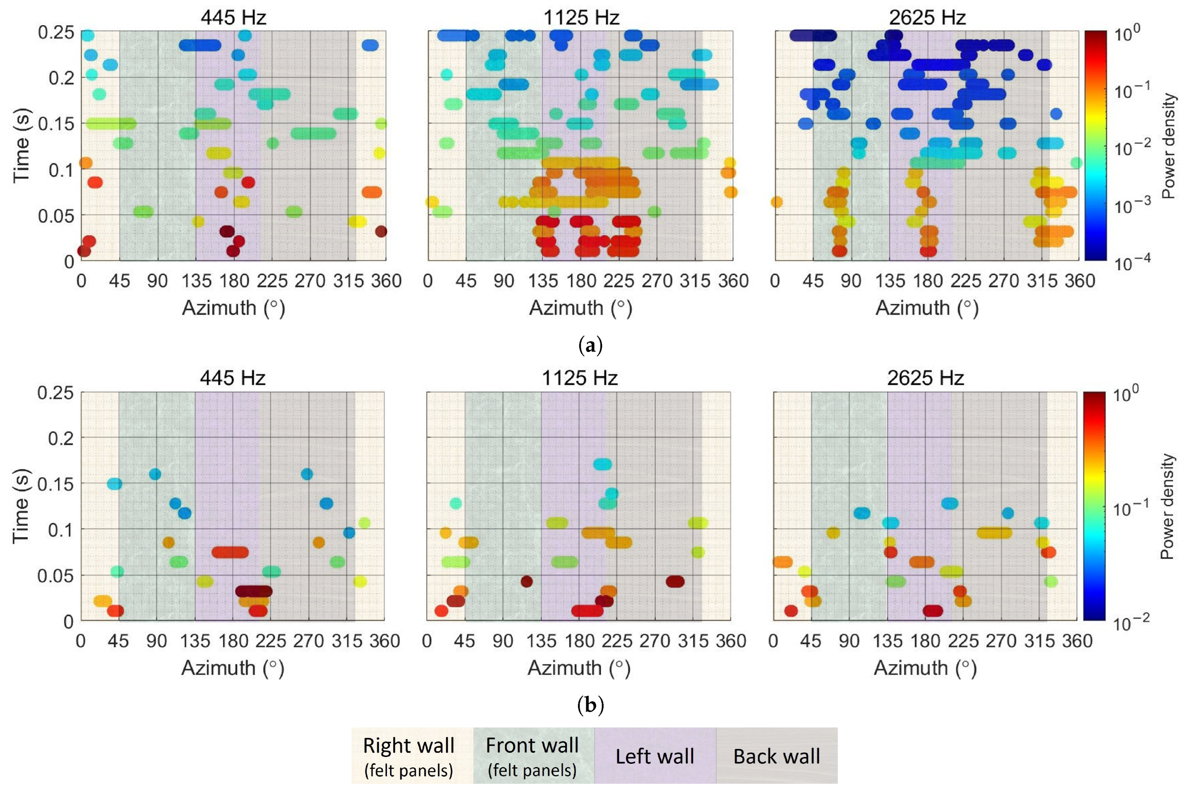
For the felt panel setting, the local azimuth maxima of $F\left(\mathfrak{X};{\mathbf{\Pi }}_{k,t|{\mathit{y}}_o}\right)$ over time for some selected frequencies based on the EM32 and NT-SF1 measurements are shown in Figure 8a and Figure 8b, respectively. In the EM32 results, high power densities are observed around ${180}^{\circ }$ (left wall) and ${360}^{\circ }$ (right wall) at 445 Hz, slightly shifted from the pattern in the wood panel environment (Figure 7a). At 1125 Hz, reflections are concentrated mostly on the left wall around $\{{135}^{\circ },{200}^{\circ },{225}^{\circ }\}$ with lower power densities compared to Figure 7a, suggesting a strong influence from the felt panels laid along the right and front walls (Figure 3b). The concentration around ${180}^{\circ }$ (left wall) and ${330}^{\circ }$ (back-right wall corner) at 2625 Hz resembles the pattern in Figure 7a, but additional strong reflections are observed around ${75}^{\circ }$ in the felt setting. After the source signal duration ($>0.1$ s), reflections appear more dispersed and weaker compared to the wood panel, especially at 1125 Hz and 2625 Hz, although some similar local maximums could be observed between Figure 7a and Figure 8a.

The NT-SF1 results in Figure 8b exhibit similar drawbacks to Figure 7b. However, the NT-SF1 is still able to detect dominant reflections around $\{{40}^{\circ }$, ${200}^{\circ }\}$ at 445 Hz, $\{{190}^{\circ }$, ${215}^{\circ }\}$ at 1125 Hz, and ${180}^{\circ }$ at 2625 Hz, which are in close proximity to the EM32 results (Figure 8a). Additionally, the secondary maxima at 445 Hz are near the corresponding directions in Figure 8a.

Across both the wood and felt panel settings, some common patterns emerge between Figure 7 and Figure 8. High power densities are consistently observed on the left and right walls, suggesting strong reflection paths. The presence of the grand piano, in particular, contributes significantly to strong early reflections in both environments.

The NT-SF1 shows comparable reliability to the EM32 in identifying dominant early reflection directions, as the recorded sound field at these instants is governed by strong sparse reflections. At low frequencies, such as 445 Hz, where both arrays rely on first-order eigenbeams, it also captures secondary reflections consistent with the EM32. However, this performance does not persist at later time instants as the reflection field becomes more complex. Even at the same eigenbeam order, the EM32 benefits from denser spatial sampling, enabling richer spatial representation and more resolved directional estimates. At higher frequencies, where higher-order eigenbeams are available for the EM32, this performance gap becomes more pronounced.

5.3. Directivity Time-Span

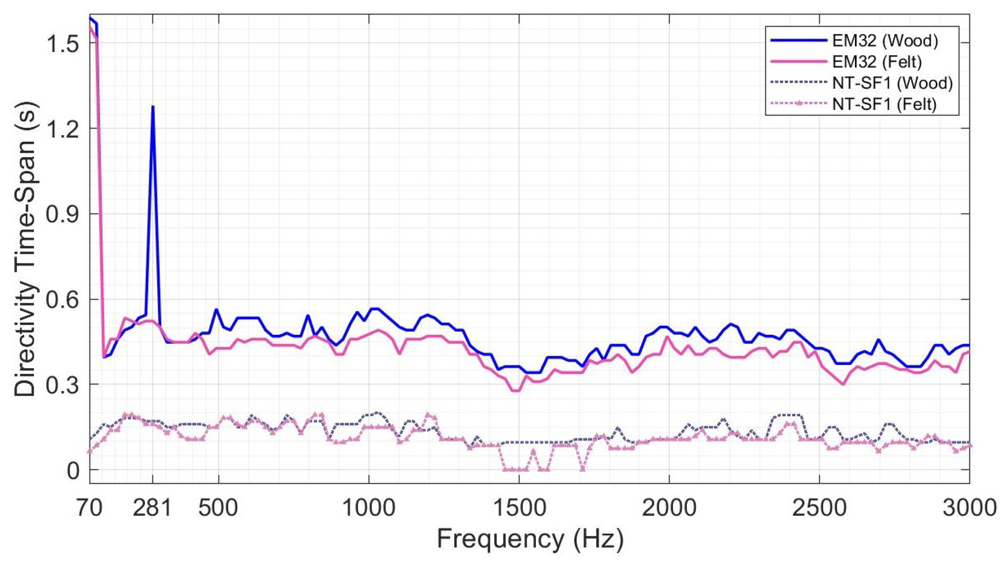
Figure 9 presents the directivity time-span across frequencies for both the wood and felt panel settings, based on measurements from the EM32 and NT-SF1. The EM32 results show the highest time-span around 70–95 Hz for both configurations, with a secondary peak around 281 Hz in the wood case. These peaks indicate sustained anisotropic reflection distributions typically associated with the resonant behavior of low-frequency room modes and their interference patterns, which lead to non-uniform energy distribution with slower temporal decay [54,55]. The felt response appears to suppress the peak at 281 Hz and shows consistently lower time-span values than the wood for frequencies beyond ≈400 Hz. This validates the increased absorption by the felt surfaces, leading to faster damping of anisotropic reflections. The directivity time-span thus provides a more informative indicator of material-dependent acoustic behavior than the aggregate power measure, which does not show any contrasts at low frequencies (see Figure 6).

In both environments, the time-span estimate by the EM32 marginally decreases toward higher frequencies (excluding the dip around $1.5$ kHz), which is expected as the sound field becomes more diffused due to increased wave scattering [54,55]. The average directivity time-span is around $0.48$ s and $0.43$ s for the wood and felt settings, respectively.

The NT-SF1 results in Figure 9 show significantly lower directivity time-span values, with a relatively flat response compared to the EM32 for both wood and felt settings. As already seen in Figure 7 and Figure 8, the NT-SF1 fails to detect directivity models when the reflected field becomes more dispersed and weaker over time. Since directivity time-span depends on the detectability of vMF clusters, this results in an underestimation of the duration of anisotropic reflection behavior.

Furthermore, the NT-SF1 results do not feature the low-frequency peaks present in the EM32 plots, even though these frequencies’ models are based on first-order eigenbeams for both arrays. On the other hand, Figure 6 shows that the NT-SF1 captured the aggregate reflection power at 281 Hz as effectively as the EM32. This disparity underscores the differences in spatial detail of the reflection field captured by the four-microphone NT-SF1 compared to the 32-microphone EM32, highlighting that agreement in the total reflection power does not imply equivalence in spatial characterization. These observations further corroborate the findings in Section 5.2 that even at the same eigenbeam order, arrays with denser microphone layouts enable more reliable tracking of anisotropic reflection structures over time.

Despite these shortcomings, the NT-SF1 indicates a lower directivity time-span in the felt environment compared to wood, especially at higher frequencies. The average directivity time-span is around $0.13$ s for the wood setting and $0.11$ s for the felt setting. Although the contrast is less pronounced than in the EM32 results, this suggests that the NT-SF1 captures sufficient spatial detail to distinguish between the two acoustic settings.

5.4. Directional Variations in Decay Time

Directions with long decay times indicate highly reflective surfaces that sustain reflection energy and contribute significantly to the late reverberant field [18,55,56]. These directions are not necessarily those of dominant early reflections with a high power density, which are primarily governed by the source–receiver positions.

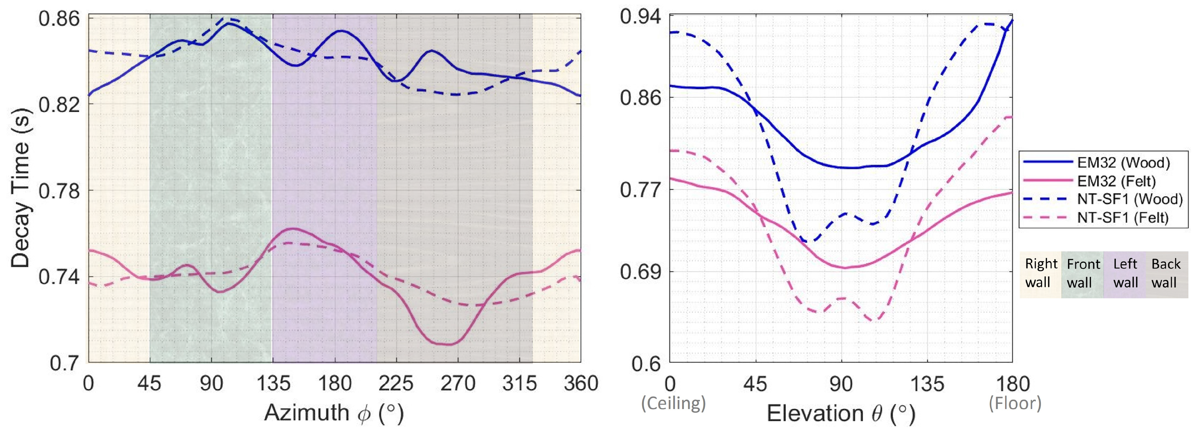
Using ${\mathcal{P}}_R(k,t,\widehat{\mathit{y}}|{\mathit{y}}_o)$ derived from the EM32 and NT-SF1 measurements, we estimated a 60 dB decay time for each $\widehat{\mathit{y}}$ direction in both the wood and felt panel settings. The decay times averaged over 0.1–1.0 kHz across the azimuth and elevation angles are shown in Figure 10. Both arrays clearly demonstrate shorter decay times for the felt setting compared to the wood. With felt panels on only two wall sections, this result highlights their effectiveness in reducing the overall persistence of reflections across the room.

In the azimuth plot, the EM32 results for the wood setting show the highest peak around ${100}^{\circ }$ on the front wall, which has highly reflective wooden panels. Secondary peaks occur around ${180}^{\circ }$ (left wall), ${70}^{\circ }$ (front wall), and ${250}^{\circ }$ (back wall), where the first two are associated with wooden surfaces and the third coincides with the glass door to the control room (Figure 3). With the felt panels, the highest peaks shift to around ${150}^{\circ }$ on the left wall and ${355}^{\circ }$ near the grand piano location, while the front and back walls exhibit relatively shorter decay times.

In the elevation plot for both the wood and felt settings, the EM32 results show peak decay times at extreme elevations and much lower values around the XY-plane ($\theta \approx {90}^{\circ }$). This behavior could be attributed to the curved plywood frames in the upper elevations ($\theta \ll {90}^{\circ }$), ceiling diffusers ($\theta \approx 0^{\circ }$), and the wooden floor ($\theta \approx {180}^{\circ }$) present in the studio (Figure 3). In the wood setting, decay times peak around the floor directions. In the felt setting, similar values are observed at extreme elevations, indicating better control of the reflection paths from the floor.

The decay time represents the cumulative effect of multiple reflection paths and boundary interactions and thus the combined influence of room surfaces on the late field. The observations indicate that the reverberant field does not exhibit isotropic decay in the presence of heterogeneous surface materials. Furthermore, localized material treatment does not uniformly scale the directional decay pattern but reshapes it through changes in the reflection paths and surface contributions.

In both azimuth and elevation plots for the wood and felt settings, the NT-SF1 shows trends similar to the EM32 but with fewer fluctuations across the azimuth, as expected from its limited spatial resolution. Notably, the highest peak directions align closely between the NT-SF1 and EM32, indicating that the NT-SF1 reliably identifies directions of prolonged decay and the associated highly reflective surfaces.

6. Practical Implications and Future Work

The comparative analysis in Section 5 highlights the applicability of the eigenbeam–vMF-based analyzer across different microphone arrays. The results indicate that the analyzer can extract meaningful acoustic features even with reduced spatial sampling, supporting its use across practical scenarios. In applications requiring detailed spatial characterization, such as architectural studies and controlled acoustic experiments, higher-order arrays remain more suitable due to their superior spatial resolution. In contrast, first-order or compact arrays provide a viable solution for initial acoustic measurements and low-cost campaigns, where identifying dominant reflection behavior, material differences, or relative acoustic changes is sufficient. This trade-off between the spatial resolution and measurement complexity underpins scalable and resource-efficient acoustic analysis.

The analyzer combines eigenbeam spatial correlation with vMF-based parameterization to provide a compact and interpretable representation of the reflection field, which can inform various downstream tasks. However, the fidelity of this representation is fundamentally constrained by the spatial resolution and finite-order ambisonic encoding supported by the measurement system. These limitations become critical in late and highly reverberant conditions, where the reflection field comprises dense and overlapping components that cannot be reliably separated in the directional domain. While parameter tuning can offer marginal improvements, the achievable level of detail is ultimately governed by the spatial information captured by the array.

The current formulation also assumes a plane wave representation of reflections, which does not account for near-field effects or complex boundary interactions in proximity to reflective surfaces. Extending the model to incorporate near-field behavior could improve its applicability in more realistic acoustic scenarios. In addition, evaluating the analyzer across a wider range of room geometries and source–receiver configurations could help assess the robustness of the observed trends.

A key challenge in this analysis is the absence of ground truth for the underlying reflection field in real-room environments, as the true propagation and interaction of sound waves are not directly observable. Consequently, the estimated directional features could not be explicitly verified. The reliability of the results is therefore inferred through consistency across arrays, agreement with the known acoustic properties of the environment, theoretical understanding, and physical interpretability. Future work will focus on developing validation frameworks using controlled measurements or simulated datasets with known parameters to quantify uncertainty and strengthen confidence in the analysis.

7. Conclusions

In this paper, we employed the eigenbeam–vMF-based analyzer to assess the acoustic properties of a recording studio with variable wall paneling using two different microphone arrays: a 32-channel SMA capable of fourth-order ambisonic capture and a first-order ambisonic array. The key findings of this study are summarized as follows:

• The spectral response, directional power density, directivity time-span, and directional decay times demonstrated the increased absorption effect of felt panels compared to wood. In particular, the felt panels led to more scattering and damping of reflections over time, suppressed the lifespan of low-frequency anisotropic reflections, and shortened the decay times.
• Both the SMA and the first-order array identified differences in the analyzed features for the two acoustic settings, with these differences being more pronounced in the SMA and more marginal in the first-order array.
• The SMA and first-order arrays displayed similar trends in the spectral response of the total received reflection power, with close overlap in the first-order frequency range, capturing consistent peak frequencies associated with modal effects and reinforcing interference patterns.
• The analysis of dominant reflection directions revealed concentrated reflections on the left and right walls, particularly around the grand piano near the back-right wall corner. The directional pattern varied between the wood and felt settings, with significant changes at certain frequencies. The first-order array could identify dominant directions and secondary reflections of low frequencies, aligning with the SMA.
• The first-order array struggled to estimate the directivity models after a few early reflections even at low frequencies, whereas the SMA captured the anisotropic features for a comparatively longer duration. Consequently, the first-order array exhibited a significantly lower directivity time-span and failed to identify prolonged anisotropic reflection fields at low frequencies as effectively as the SMA.
• The analysis of decay time variations over directions indicated highly reflective surfaces. Both the SMA and first-order array exhibited similar trends, with closely aligned highest peak directions.

This study highlights the distinct acoustic characteristics of the recording studio under different panel settings and the relative effectiveness of different microphone arrays in capturing these characteristics using the eigenbeam–vMF-based analyzer. The SMA captured the finer spatial details of the anisotropic reflection field, making it suitable for high-precision acoustic analysis. While the first-order array has limited capabilities compared to the SMA, it is still useful for preliminary analysis of the room acoustics. It effectively distinguished acoustic environments and identified key acoustic features such as the room modes, dominant early reflection directions, and highly reflective surfaces. However, it cannot be relied on for detailed analysis of directional features across a wider time–frequency spectrum. These findings enhance our understanding of room acoustic analysis using the eigenbeam–vMF analyzer, providing valuable insights into the practical applications of various microphone arrays in complex acoustic settings.