Application of Computer Simulation to the Multidimensional Profit Optimization for the Paper Production Process, Taking into Account Thermal and Electrical Energy Consumption

Abstract

The paper presents the results of the optimization of the paper production process as a function of paper grade, basis weight and key operating parameters of paper machines, wire speed V_s and reel speed V_n, using computer simulation. Based on empirical data from 2015 to 2020, the analysis accounts for web breaks, downtimes, and grade changes, all of which affect production continuity and the operation of the plant’s combined heat and power (CHP) system supplying thermal and electrical energy. Production interruptions reduce CHP stability; therefore, the optimization criterion was profit maximization, including energy-related effects associated with forecasting the availability of surplus energy for sale when participating in the capacity market. The results were compared with those obtained using numerical taxonomy methods, which confirmed the effectiveness of their application to the problem under consideration.

1. Introduction

The paper and pulp industry has contributed to air and water pollution by utilizing resource-intensive processes, such as water, energy, and chemicals, which have had a substantial impact on the environment. Furthermore, the ecosystem is severely impacted by the deforestation this industry causes, which results in soil erosion, a decline in biodiversity, and an increase in greenhouse gas emissions. Decomposition of substantial waste can be protracted and can result in additional environmental damage. Another issue is that the paper industry is confronted with substantial operational challenges, such as fluctuations in demand that are influenced by environmental awareness, uncertainties in raw material availability, and regulatory and resource constraints [1]. That is why an efficient prediction tool is required to obtain trustworthy forecasts regarding profits and costs as well energy production details, if required.

Computer simulation is currently a tool used in a wide range of optimization problems. It has developed in parallel with the progress of computers and software. Its principles have been presented many times in various scientific studies, taking into account the wide spectrum of analyses it offers together with the rapid development of information technology and computational capabilities [2,3,4]. It was first used on a large scale during World War II to model the process of nuclear detonation [4]. Many studies have also addressed the problem from an epistemological perspective [5,6,7]. After 1990, computer simulation developed in a leap-like manner [8,9,10] and now has wide applications in various fields. Its usefulness in solving different optimization problems has been demonstrated in numerous works, including those presenting its general capabilities [11,12]. The use of MATLAB Simulink and Simscape Multibody software for this purpose is a popular solution [13]. Comparisons between computer simulation and different computational techniques are discussed in [14]. Typical applications of computer simulation include, for example, the aerospace industry, where it is used, among others, to determine the aerodynamic characteristics of aircraft structures (airplanes, rockets) [15]. Another application is the support of command and control processes in air defense [16].

Computer simulation is also used in medicine, for instance in the treatment of various types of cancer, including for planning chemotherapy and radiotherapy [17,18,19,20]. Applications in economics can be found in studies [21,22,23], which present so-called experimental economics. Another example is the economic optimization of zeolite production using the Monte Carlo simulation method [24]. Furthermore, it is also possible to use computer simulations in the training of social work professionals [25]. Optimization of complex production processes and issues related to production management are discussed in [26,27,28]. The issue of CO₂ emissions optimization and related production considerations was discussed in the paper by Pawlak and Satarnus [29]. This approach was also presented from the perspective of a decision-maker responsible for managing the production process [30], as well as for determining the values of selected process parameters that ensure the achievement of a specific objective [31]. The issue of production time optimization using computer simulation can be considered from various perspectives, but the most common criterion is profit maximization [32,33]. Issues related to production logistics (regarding time, but also other aspects) are also common criteria. A logistics criterion can be multifaceted, taking into account many factors simultaneously [34]. The same applies to the issues of production planning and the selection of appropriate tools for it [35].

Additionally, computer simulation can be effectively used for the optimization of a combined heat and power plant’s production schedule when fired with natural gas, with the aim of maximizing the total gross margin in the day-ahead horizon of CHP plant operation [36,37,38]. The use of the Minimax rule in this context is presented in [39]. Multidimensional optimization problems related to energy consumption have also been discussed in other works [40,41,42], including studies that take energy storage into account [43,44]. Reviews of research in this area can be found in numerous scientific publications [45,46].

In connection with growing cybercrime and competition between states in cyberspace, many studies have been devoted to describing the life cycle of a cyberattack [47,48], including approaches using Markov chains to model this cycle [49,50]. Computer simulation is also used in the optimization of general storage processes, estimated on the basis of current or predicted data [26,43,51].

The business activity of one of the largest paper mills in Poland consists, in addition to paper production, in generating heat and electricity for internal consumers within the mill itself, as well as for neighboring customers. The priority of the company is to supply the MP1 and MP2 paper machines, which require a sufficient amount of energy at all times.

In order to enable the sale of surplus generated energy on the power exchange, accurate forecasting of heat and electricity production is required. However, the system is unstable due, among other factors, to so-called “web breaks” of the produced paper reel, which hinder such forecasting by reducing the amount of heat and electricity available in the system. Minimizing interruptions in the operation of the paper machine improves the continuity of paper production and, as a consequence, positively affects the quality of forecasts of the amount of generated heat and electricity.

On the basis of historical data from the considered plant for the years 2015–2020, an optimization of paper production was carried out as a function of paper grade, basis weight, and the main operating parameters of the paper machine, i.e., wire speed V_s and reel speed V_n for individual years. In [52], optimization based on numerical taxonomy was presented. The aim was to identify such ranges of V_s and V_n that the probability of paper production (P₁) would be maximized, while the probabilities of downtime (P₂), grade change (P₃) and web break (P₄) would be minimized. This was achieved by maximizing the distance of the normalized probability vector (after converting the stimulant P₁ into the destimulant Q, i.e., its reciprocal) from the pattern vector.

The primary objective of the research was to optimally select the operating parameters of the paper machine (V_s and V_n) in order to minimize the number of so-called “breaks” in the paper roll, which has a direct impact on the stability of the system and the accuracy of predictions regarding the amount of heat and electricity produced by the system. The optimization criteria were profit maximization and the corresponding optimal production time (for individual ranges of V_s and V_n). The optimal values of the V_s and V_n ranges were obtained by comparing the optimal production times (for all ranges studied). The studies were carried out for each year, a specific type of paper produced (including its thickness) and each of the two paper machines (MP1 and MP2).

2. Methodology

In the production plant under consideration, heat and electricity are generated in a gas–steam cogeneration (combined heat and power, CHP) system. The main advantage of cogeneration is that surplus heat is used for useful purposes instead of being released into the environment. This brings a number of benefits [36], such as reduced emissions of harmful greenhouse gases, which in turn lowers the costs of purchasing emission allowances. Other advantages include increased efficiency of energy generation and reduced production costs.

The primary task of this CHP plant, located in western part of Poland is to ensure the continuous operation of the MP1 and MP2 paper machines installed in the mill which can work independently or in a shift mode. Surplus generated energy is directed to the plant’s own needs and to external consumers.

As the company plans to sell surplus energy on the market, there is a need to forecast the amount of heat and electricity generated by the system. However, the production process is influenced by random phenomena, the probability of which has become one of the key criteria in forecasting the declared amount of electricity generated at any given time.

The problem is the instability of the system caused by “breaks” of the produced paper reel, which force the paper machine to stop and vent steam. In order to keep the steam turbines running (or to reduce their power), the steam vented by the machine is redirected to specially designed blow-off lines, which reduces the amount of heat and electricity available for sale. As a result, prediction of the amount of heat and electricity generated by the system is significantly hindered. To improve system stability and the accuracy of forecasts, the number of web breaks and the resulting downtime of the paper machine must be minimized.

2.1. Computer Simulation

Computer simulation is a process of experimentation on a virtual mathematical model representing a real object or phenomenon [2,3,4]. In such a process, three essential stages can be distinguished: preparation of the model (pre-processing), execution of calculations, and analysis of results (post-processing).

A computer program was developed specifically for this purpose to carry out the calculations. It was written in C++, and no specialist simulation libraries were used. The method used to perform the calculations is described in the following section.

2.2. Basis for the Calculation

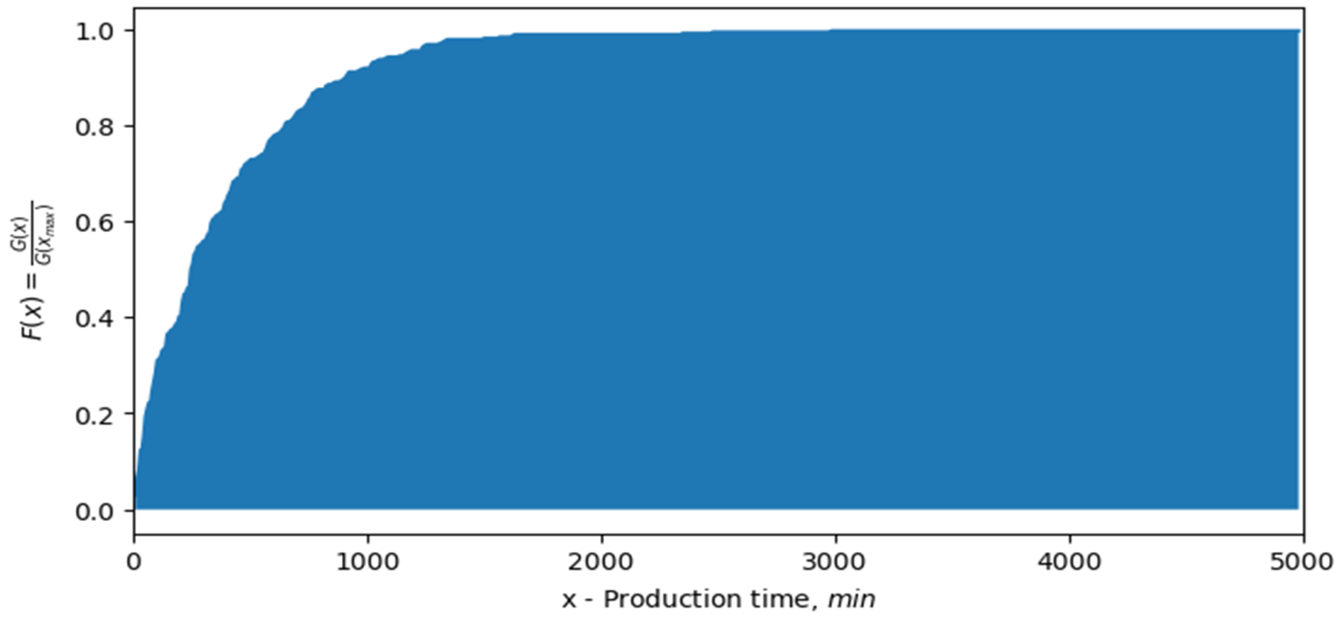
The first stage of the calculations involves computing the cumulative distribution function of the probability distribution. To this end, the probability density function for time to web break was calculated based on the actual data available. The calculated density function represents the relationship between production time and the probability of a breakdown occurring. The first step in calculating the probability density function of breakdown time is to initialize the array in which the values of the discrete probability density function will be stored. The array consists of a specific number of elements, which must be specified. In this case, it has been assumed that this will be the maximum production time until a break occurs, denoted in the algorithm as MAX_PRODUCTION_TIME. Next, in a loop for each sample relating to the given paper and falling within the assumed speed ranges, a check is made to see if a break has occurred. The program records the number of minutes after which it occurred, and for that time (the corresponding position on the x-axis), the value on the y-axis is incremented by one. The function calculated in this way does not satisfy the properties of a probability density function, as its integral, calculated over the entire accepted space of elementary events, is not equal to 1. As indicated in the previous description, the assumed space is a discrete space and constitutes a set of integers in the range from zero to MAX_PRODUCTION_TIME.

The cumulative distribution function was calculated on the basis of the unscaled probability density function obtained in this way. According to the definition, the cumulative distribution function is given by Equation (1).

$$\mathrm{F}\left(\mathrm{x}\right)={\int }_{-\mathrm{\infty }}^{\mathrm{x}}\mathrm{f}\left(\mathrm{x}\right)\mathrm{d}\mathrm{x}$$

(1)

where f(x) is the probability density function.

In the discrete case, the value of the cumulative distribution function at a given point in the table is the sum of the values in the table describing the probability density function from its start to that point. Finally, the result obtained must be rescaled so that the property of the cumulative distribution function is satisfied, i.e.,

$$\underset{\mathrm{x}\to \mathrm{\infty }}{\lim }\mathrm{F}\left(\mathrm{x}\right)=1$$

(2)

In the discrete case it is sufficient to divide each value in the array describing the distributive function by the last element of that array.

2.3. Simulation Algorithm

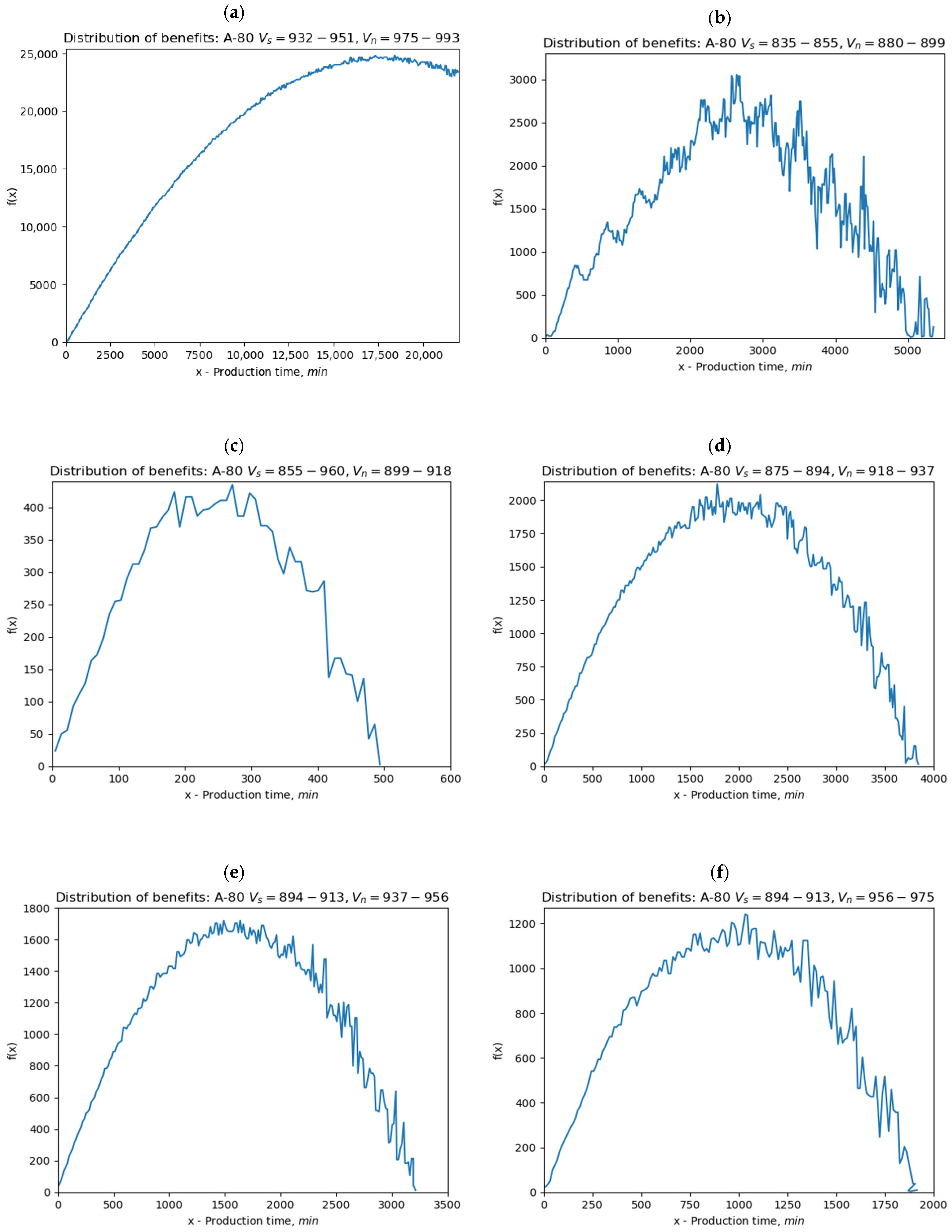
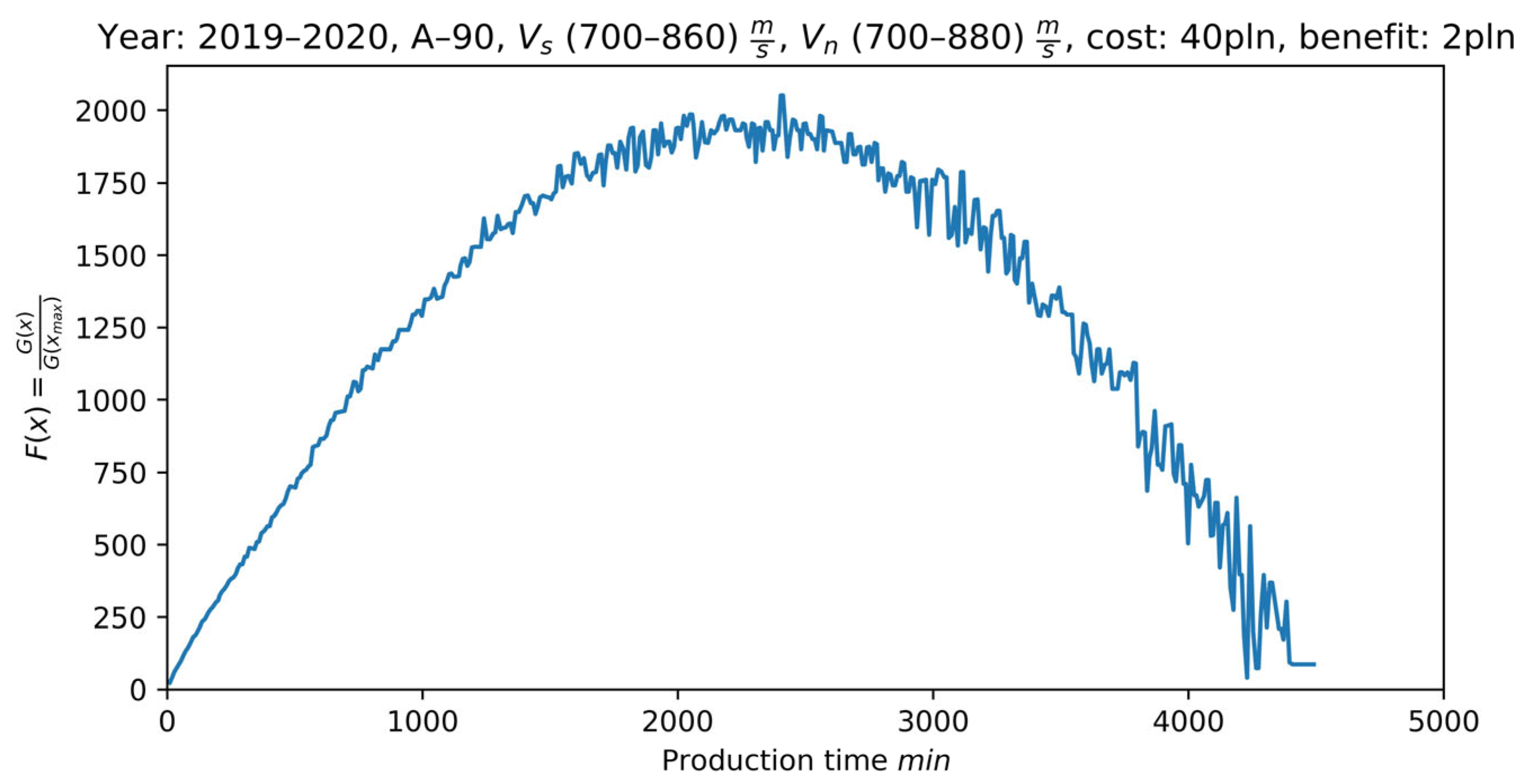
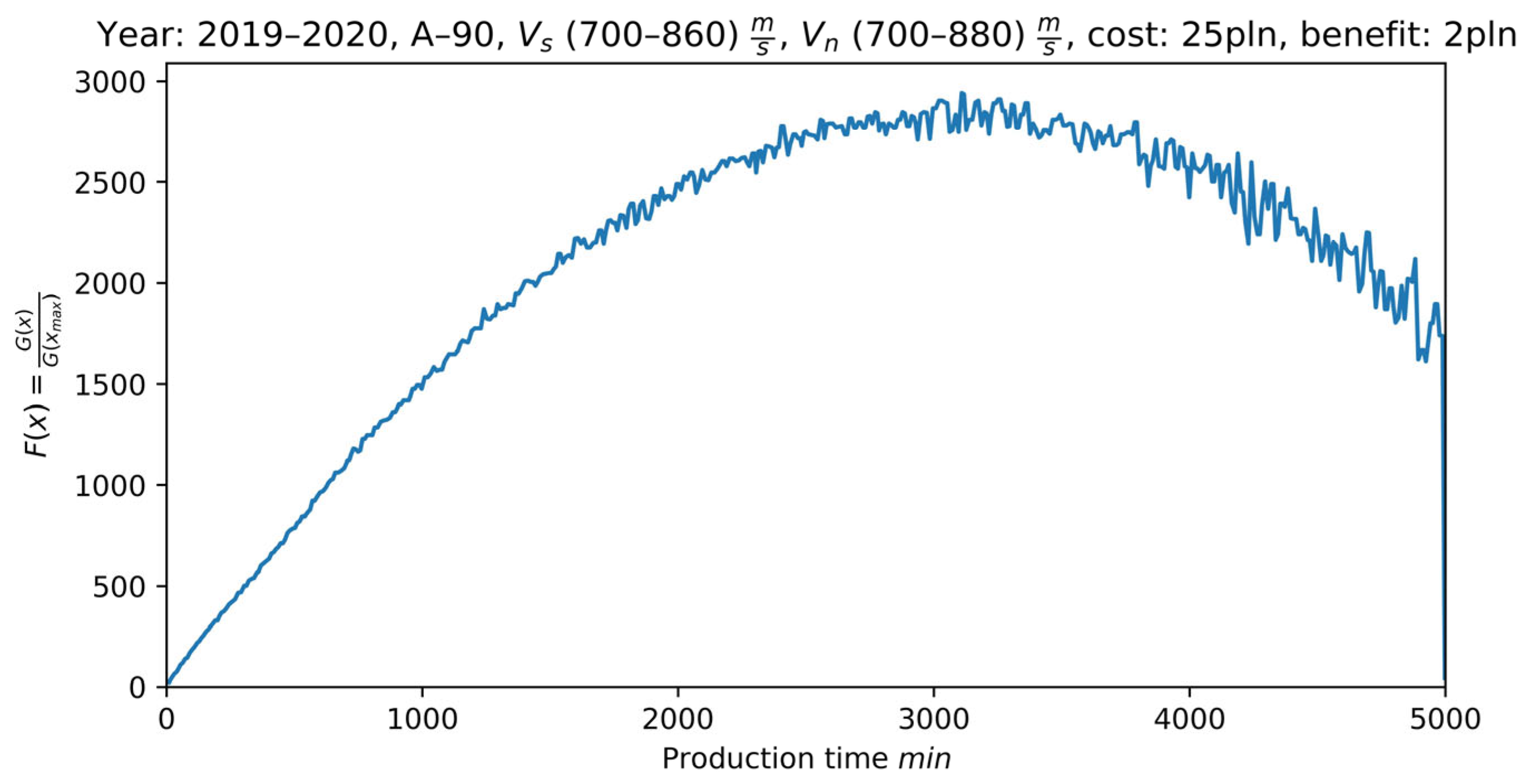
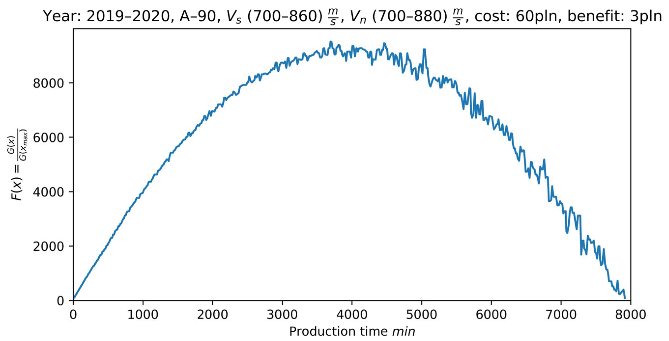
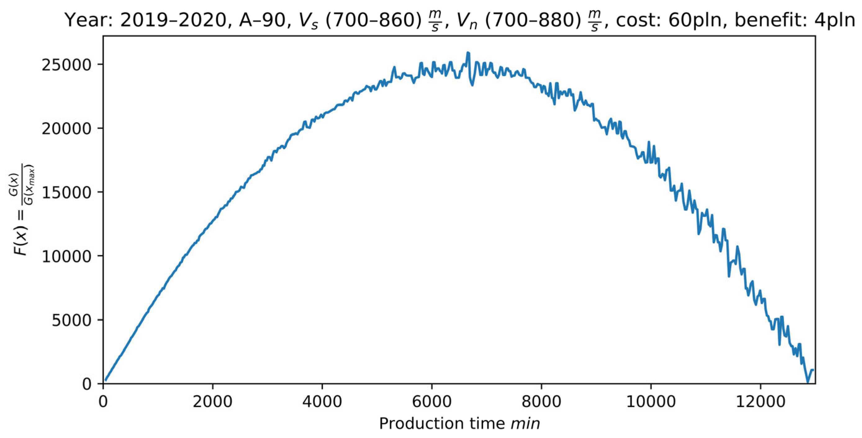
The simulation was carried out based on the distribution function described earlier. The simulation was conducted separately for each type of paper and for the selected range of speeds V_s and V_n. Within a loop, the profit obtained from the simulation was calculated for every possible, specified production time. To this end, the profit was first calculated for a production time of 0, then for production times of 1, 2, 3, 4, up to the assumed MAX_PRODUCTION_TIME. This yielded a graph showing the relationship (function) between profit and production time. Based on the obtained function, it is possible to determine the production time at which the greatest profit is achieved for the given parameters. This is the value at which the function reaches its maximum (extremum).

The basis for the simulation calculations is a random value for the time to failure. In many systems, a typical probability distribution is assumed, such as a uniform or normal distribution. To obtain a model closer to reality, a probability distribution derived directly from actual data was adopted. This approach was used in the program described. Therefore, pseudo-random values for the time to failure were obtained in accordance with the probability distribution calculated in Section 2.2 using the method of inverting the cumulative distribution function. These values were obtained by first generating a pseudo-random value y in the range from 0 to 1, in accordance with the uniform probability distribution. Next, based on the obtained cumulative distribution function, the value x was determined for which the cumulative distribution function takes the value y. In this way, pseudo-random values of the TIME_TO_SPURT (time to web break) variable were obtained, consistent with the probability distribution resulting from the previously obtained cumulative distribution function.

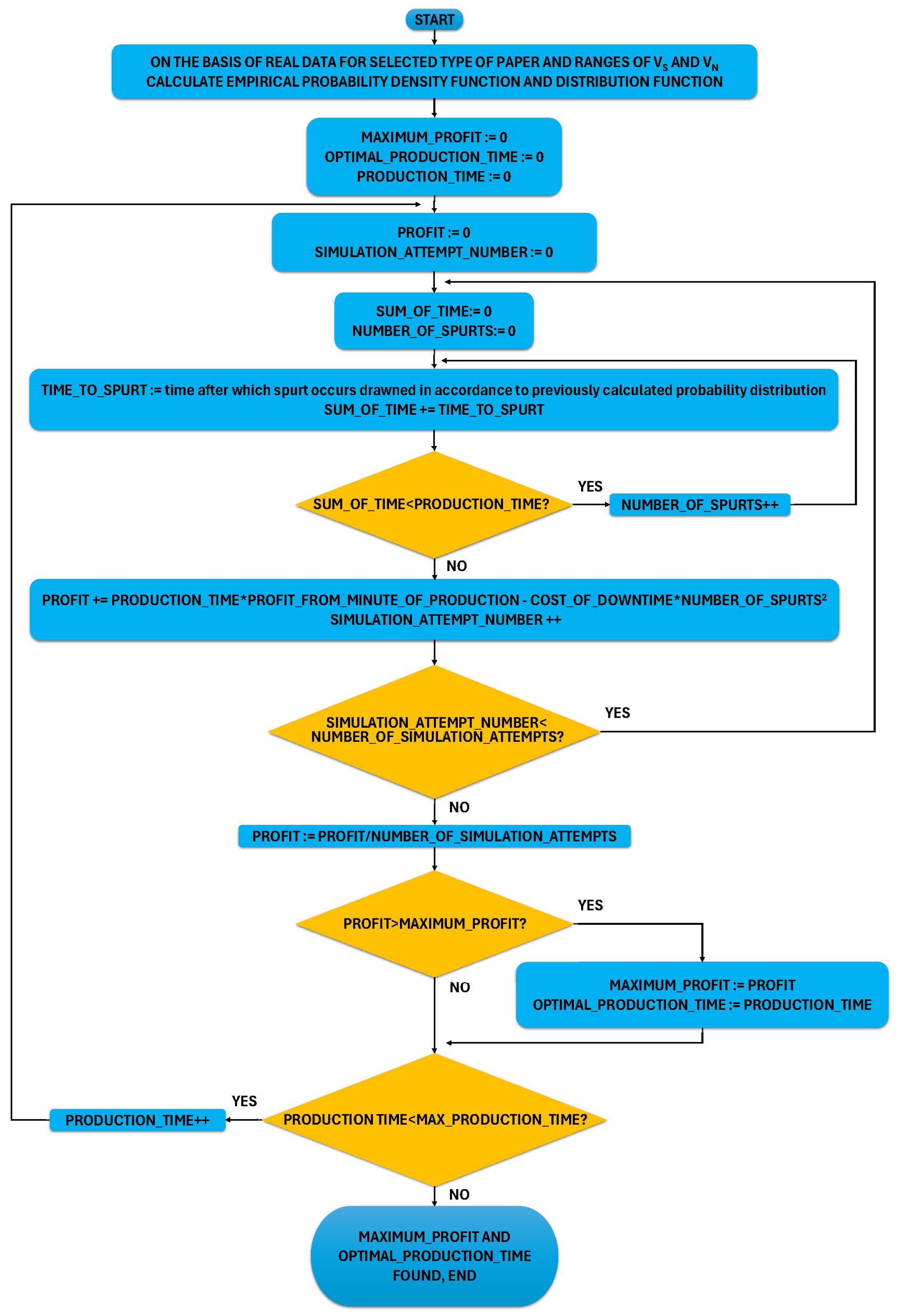
The simulation ran in two loops: an outer loop and an inner loop. The detailed algorithm is shown in Figure 1. In the outer loop, the production time was iterated; that is, the variable PRODUCTION_TIME took values ranging from 1 to MAX_PRODUCTION_TIME. The inner loop is used to repeatedly count the number of bursts resulting from the value of the PRODUCTION_TIME variable adopted in the outer loop. The inner loop is executed as many times as the value of NUMBER_OF_SIMULATION_ATTEMPTS. The number of bursts is calculated by generating a random value for TIME_TO_SPURT until the sum of these times is greater than or equal to the PRODUCTION_TIME variable. When this occurs, the number of spurts is directly determined by how many times the function generating the random value TIME_TO_SPURT had to be called. The number of bursts is stored in the variable NUMBER_OF_SPURTS. Once the number of breaks has been calculated for a given production time, based on the previously calculated distribution function, the profit obtained for the given parameters and random values is calculated. For the simulation calculations, Equation (3) was used:

$$\mathrm{z}={\mathrm{x}}_{\mathrm{p}}·{\mathrm{k}}_{\mathrm{m}\mathrm{p}}·{\left({\mathrm{l}}_{\mathrm{z}\mathrm{r}}\right)}^2· {\mathrm{s}}_{\mathrm{p}}$$

(3)

where z—production profit; x_p—production time; k_mp—profit from one minute of production; l_zr—number of web breaks; s_p—cost of downtime caused by a web break.

The formula above assumes that profit is directly proportional to production time multiplied by the benefit derived from each minute of production, and decreases in proportion to the square of the number of production stoppages multiplied by the cost of downtime. This formula was derived based on expert knowledge obtained from those responsible for production planning at the company under study.

A schematic diagram of the algorithm is shown in Figure 1.

3. Experiment

The study was based on historical data from the plant under investigation for the years 2015–2020. For each paper basis weight, the maximum ranges of variation in V_s and V_n were determined, and then each of these ranges was divided into six equal parts (subranges). For example, for paper grade A-80 in 2020 it was assumed that the considered ranges of wire speed V_s and reel speed V_n could only be those subranges for which specified types of events occurred. The considered ranges are shown in

Table 1. Ranges of wire speed V_s and reel speed V_n for paper A-80 in 2020.

A-80, Year 2020
Vs [m/s] Vn [m/s]	I [835–854]	II [855–874]	III [875–893]	IV [894–912]	V [913–931]	VI [932–950]
880–898 (1)	////////////////////////
	////////////////////////
	////////////////////////
	////////////////////////
899–917 (2)		/////////////////////////
		/////////////////////////
		/////////////////////////
		/////////////////////////
918–936 (3)		/////////////////////////	/////////////////////////
		/////////////////////////	/////////////////////////
		/////////////////////////	/////////////////////////
		/////////////////////////	/////////////////////////
937–955 (4)				/////////////////////////
				/////////////////////////
				/////////////////////////
				/////////////////////////
956–974 (5)				/////////////////////////	/////////////////////////
				/////////////////////////	/////////////////////////
				/////////////////////////	/////////////////////////
				/////////////////////////	/////////////////////////
975–992 (6)					/////////////////////////	/////////////////////////
					/////////////////////////	/////////////////////////
					/////////////////////////	/////////////////////////
					/////////////////////////	/////////////////////////

(shaded part).

3.1. Empirical Distribution Function

The sample space of elementary events is the set of possible production times until a web break occurs; these are integer values from zero to x_max, where x_max is the maximum production time until a web break.

In the implemented program, the empirical distribution function was determined in a loop for each sample corresponding to a given paper grade (for fixed ranges of speeds V_s and V_n), checking whether a web break occurred. The program recorded after how many minutes it occurred, and for that time, i.e., the corresponding value on the OX axis, the value on the OY axis was increased by 1. For each sample, time (in minutes) was counted from zero until the occurrence of a web break.

As a result, a function g(x) was obtained, representing the number of web breaks as a function of production time, and then a function G(X) was constructed as the cumulative number of web breaks as a function of production time:

$$\mathrm{G}\left(\mathrm{x}\right)={\sum }_{{\mathrm{x}}_{\mathrm{i}}<\mathrm{x}}\mathrm{g}\left({\mathrm{x}}_{\mathrm{i}}\right)$$

(4)

Furthermore, the following value was calculated:

$$\mathrm{G}\left({\mathrm{x}}_{\mathrm{m}\mathrm{a}\mathrm{x}}\right)={\sum }_{{\mathrm{x}}_{\mathrm{i}}<{\mathrm{x}}_{\mathrm{m}\mathrm{a}\mathrm{x}}}\mathrm{g}\left({\mathrm{x}}_{\mathrm{i}}\right)$$

(5)

Next, a function f(x) was determined, representing the frequency of web breaks as a function of production time:

$$\mathrm{f}\left(\mathrm{x}\right)={\displaystyle \frac{\mathrm{g}\left(\mathrm{x}\right)}{\mathrm{G}\left({\mathrm{x}}_{\mathrm{m}\mathrm{a}\mathrm{x}}\right)}}$$

(6)

Finally, the desired empirical distribution function was obtained:

$$\mathrm{F}\left(\mathrm{x}\right)={\displaystyle \frac{\mathrm{G}\left(\mathrm{x}\right)}{\mathrm{G}\left({\mathrm{x}}_{\mathrm{m}\mathrm{a}\mathrm{x}}\right)}}$$

(7)

It is presented in Figure 2.

3.2. Simulation

The simulation was carried out on the basis of the empirical distribution function described in Section 3.1 (separately for each paper grade and basis weight, for the given ranges of speeds V_s and V_n). The basis of the simulation calculations is the pseudorandom value x_zr of the time to a web break, generated in accordance with the probability distribution presented in Section 3.1.

In the computer simulation-based study, the number of simulation trials was set to 1500. The large number of trials makes it possible to achieve high accuracy while not leading to excessively long computation times.

First, a pseudorandom value y was generated in the range from 0 to 1, according to the uniform probability distribution. Then, using the empirical distribution function, a value, x, was determined such that the distribution function takes the value y, i.e.,

$$\mathrm{y}=\mathrm{F}\left(\mathrm{x}\right)$$

(8)

In this way, pseudorandom values of the variable x_zr were obtained.

The simulation was executed in two loops: an outer loop and an inner loop. In the outer loop, the production time x_p, was iterated, i.e., the variable x_p took successive integer values from 1 to x_smax, where x_smax is the maximum production time in the simulation. In the developed program, the parameter x_smax is set in the “parameters” option.

The inner loop serves to repeatedly count the number of web breaks for each value of the production time parameter x_p set in the outer loop. The inner loop is executed as many times as the number of simulation trials (a value also set in the “parameters” option of the developed program) for determining the number of web breaks. First, a pseudorandom value x_zr (time to a web break) is generated on the basis of the empirical distribution function, and this is repeated until the sum of these times exceeds the value x_p (production time) specified in the outer loop. When this happens, the number of web breaks is equal to the number of calls to the function generating the pseudorandom value x_z.

Specifically, if

$${\sum }_{\mathrm{i}=1}^{\mathrm{n}}{\left({\mathrm{x}}_{\mathrm{z}\mathrm{r}}\right)}_{\mathrm{i}}={\mathrm{x}}_{\mathrm{p}}$$

(9)

then the number of web breaks is

$${\mathrm{l}}_{\mathrm{z}\mathrm{r}}=\mathrm{n}$$

(10)

On the other hand, if

$${\sum }_{\mathrm{i}=1}^{\mathrm{n}}{\left({\mathrm{x}}_{\mathrm{z}\mathrm{r}}\right)}_{\mathrm{i}}>{\mathrm{x}}_{\mathrm{p}} \mathrm{and} {\sum }_{\mathrm{i}=1}^{\mathrm{n}-1}{\left({\mathrm{x}}_{\mathrm{z}\mathrm{r}}\right)}_{\mathrm{i}}<{\mathrm{x}}_{\mathrm{p}}$$

(11)

then

$${\mathrm{l}}_{\mathrm{z}\mathrm{r}}=\mathrm{n}-1$$

(12)

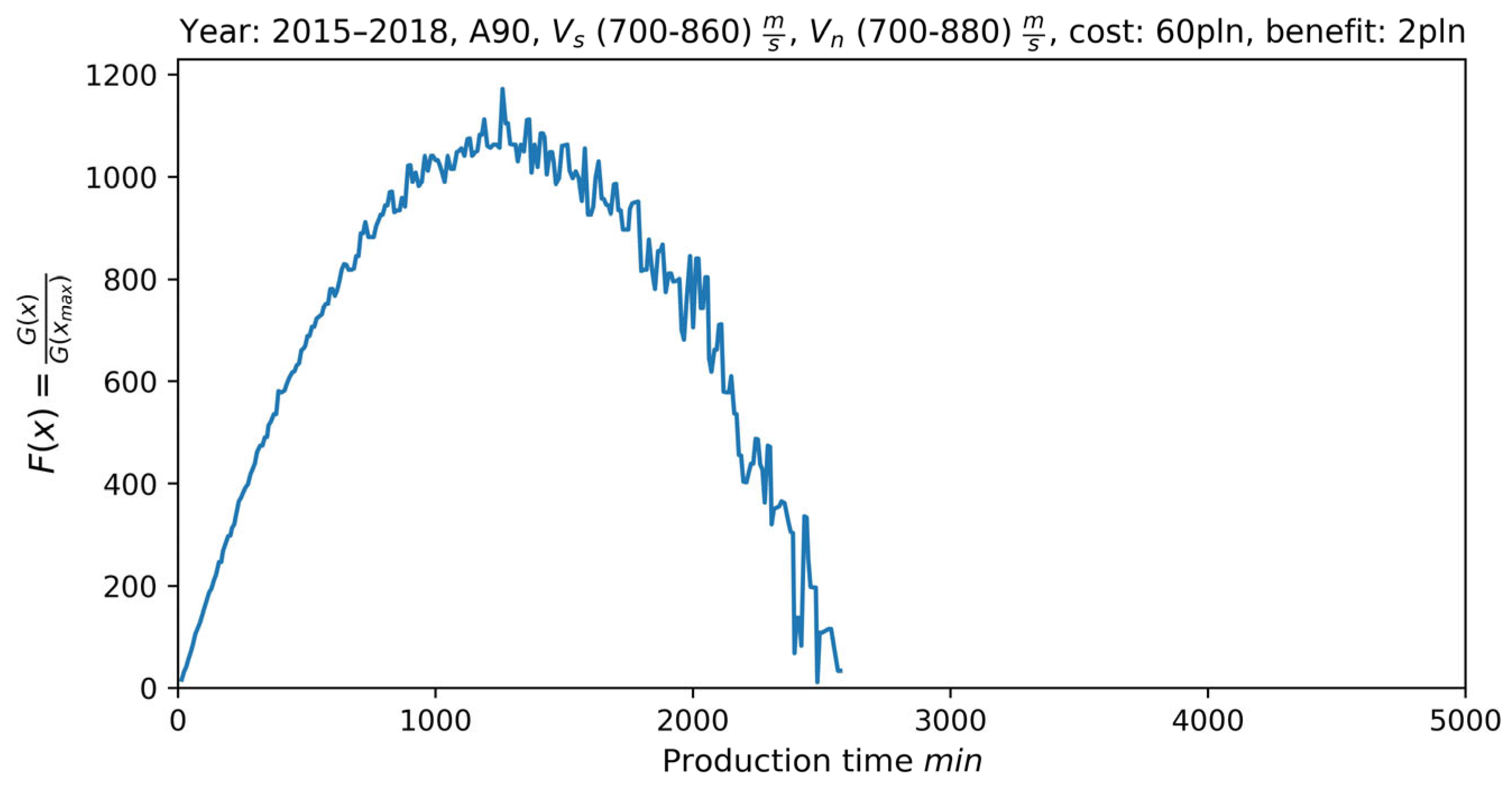
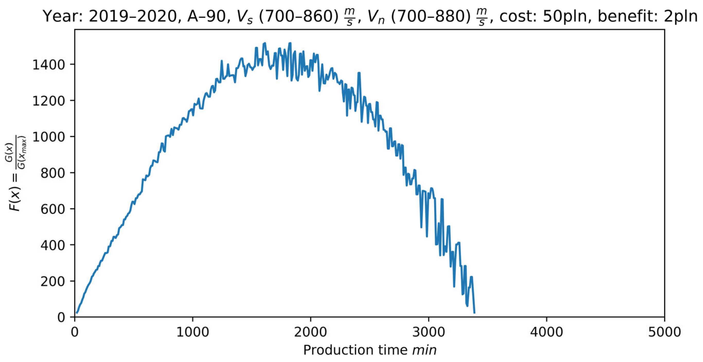
According to Formula (3), profit is the product of the production time (set in the outer loop) and the profit per minute of production, reduced by the product of the square of the number of web breaks and the cost of downtime. Thus, for each value of the variable x_p set in the outer loop, the profit resulting from the performed simulations is obtained. As a result, a functional relationship between profit and production time is obtained.

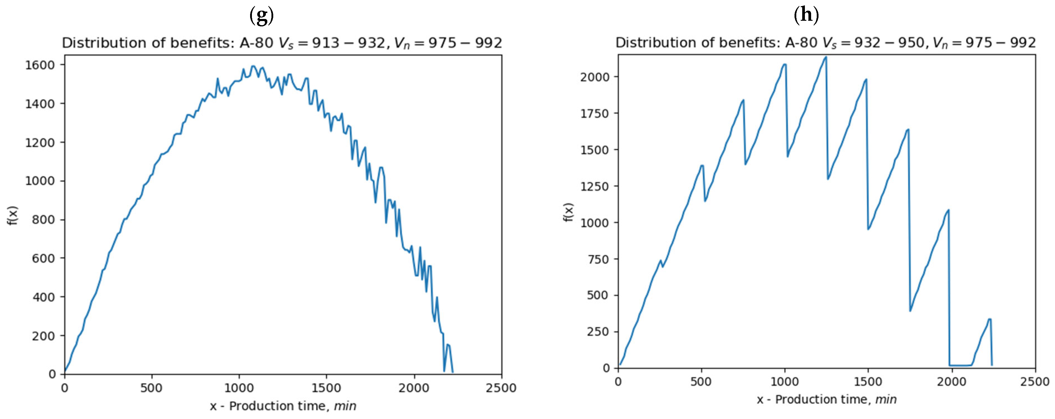
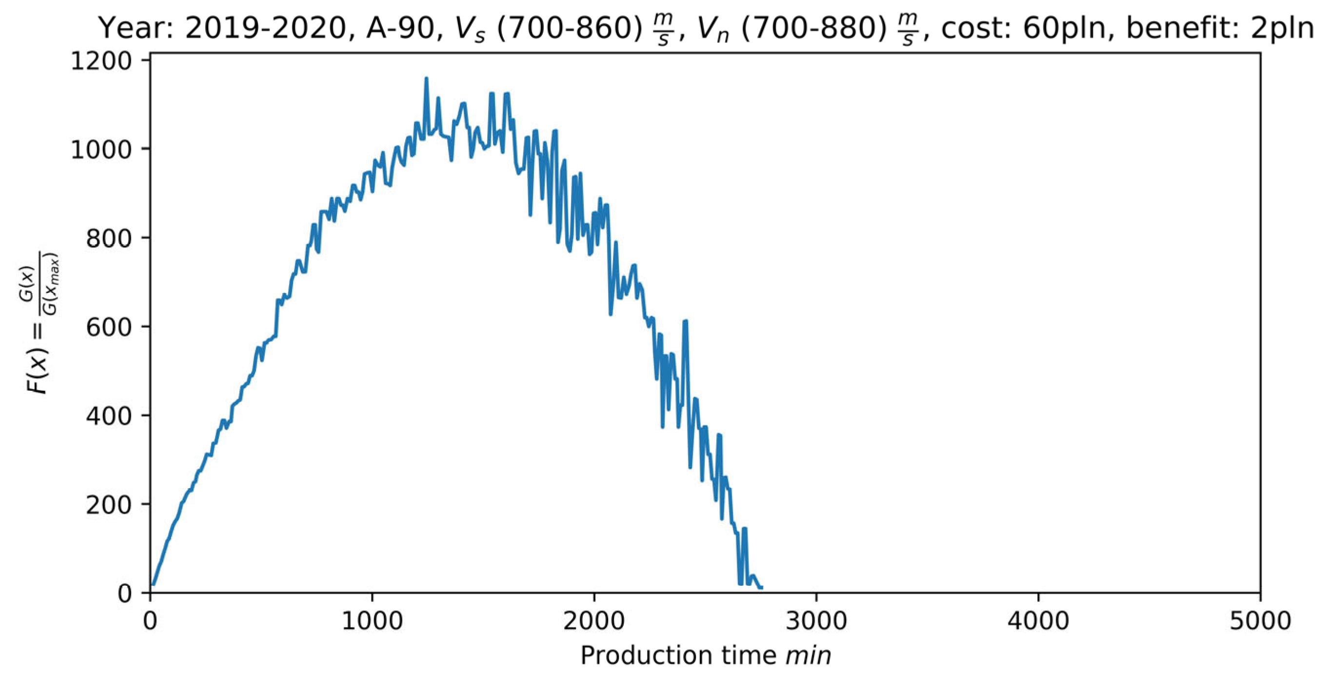
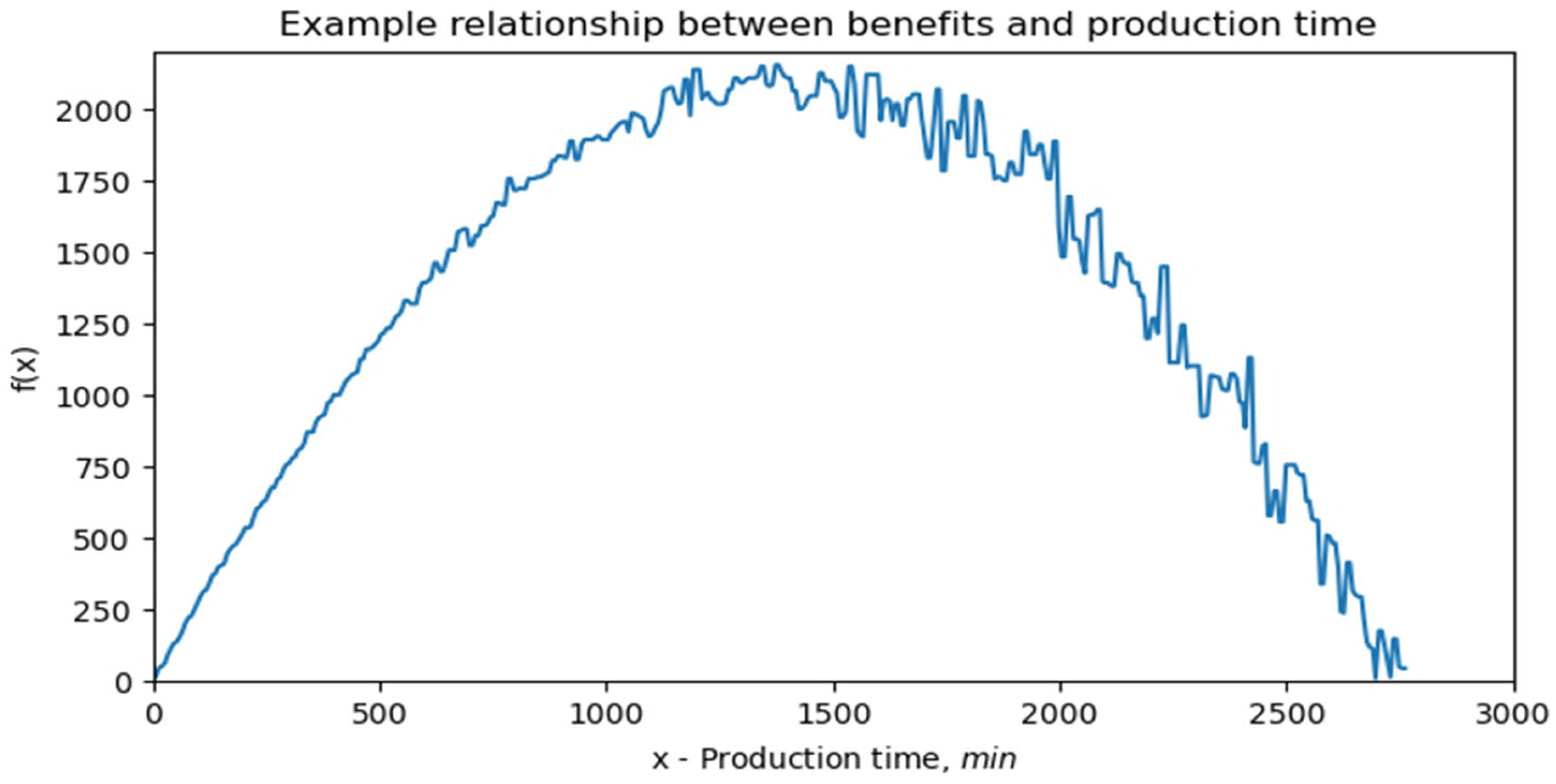
An example plot of this relationship is shown in Figure 3, presenting the obtained optimal production time equal to 1346 min with profit equal to 2181.93 PLN for paper A-70.

On the basis of this relationship, it is possible to determine the optimal production time at which the maximum profit is obtained (for the adopted parameters).

As a result of the optimization procedure described above, for a given paper grade and basis weight in a given year, and for the considered ranges of V_s and V_n, the optimal production time corresponding to the maximum profit was determined.

All calculations used to determine the empirical distribution function, as well as to perform the simulation runs (for the selected paper within specific ranges of speeds V_s and V_n) based on the chosen parameters, were implemented in a dedicated computer program developed for this purpose.

4. Results and Discussion

The results of the simulation calculations for paper A-80 on machine MP1 for the year 2020 are presented in Figure 4a–h.

4.1. Statistical Verification of the Results Obtained for the Optimal Production Time

Confidence intervals were calculated for the determined optimal production times, assuming a confidence level of 1 − α = 0.95. The results are summarized in

Table 2. Summary of optimal production times for screen speed and winding speed ranges, including confidence intervals. (1 − α = 0.95).

Optimal Production Time [min]	Vs [m/s]	Vn [m/s]	Standard Deviation	Standard Error	Confidence Interval
17271	[932, 951]	[975, 993]	5800	150	[16977, 17565]
2638	[835, 855]	[880, 899]	879	23	[2594, 2682]
274	[855, 875]	[899, 918]	100	3	[269, 279]
1756	[875, 894]	[918, 937]	585	15	[1726, 1786]
1545	[894, 913]	[937, 956]	515	13	[1519, 1571]
1022	[894, 913]	[956, 975]	341	9	[1004, 1040]
1069	[913, 932]	[975, 992]	356	9	[1051, 1087]
1250	[932, 950]	[975, 992]	417	11	[1229, 1271]

. The analysis is characterized by high statistical precision, and the determined optimal points are very stable. Even in Figure 4h, which shows the most visually “jagged” simulation, the result obtained is highly reliable within a narrow range. In all cases, the margin of error was approximately 1–2 [%], which is due to the large number of trials, which smooths out the variation shown in Figure 4a–h. Particularly for low values of the optimal production time for a given paper type and the resulting profit, the simulated values are very precise and the risk of a paper roll break is low for them. In case 4a, the optimal time is very long. This is due to the relatively low probability of breakage for the selected V_s and V_n values. However, this may be the result of insufficient empirical data for these ranges, and thus the obtained value of the optimal production time may be unrealistic to achieve in practice. For the remaining cases, the values of the optimal production times are entirely realistic, having occurred repeatedly in practice during the studied period of 2015–2020.

4.2. A Comparison of Computer Simulation Results Obtained Using the Numerical Taxonomy Method

Another approach adopted for the subject under study involved the use of taxonomic methods based on Euclidean metrics, which enabled the multidimensional analysis and classification of data on the basis of their quantitative characteristics. In [52], a normalized vector was defined:

$$\mathrm{v}=\left({\displaystyle \frac{\mathrm{Q}}{{\mathrm{Q}}_{\mathrm{m}\mathrm{a}\mathrm{x}}}},{\displaystyle \frac{{\mathrm{P}}_2}{{\mathrm{P}}_{2\mathrm{m}\mathrm{a}\mathrm{x}}}},{\displaystyle \frac{{\mathrm{P}}_3}{{\mathrm{P}}_{3\mathrm{m}\mathrm{a}\mathrm{x}}}},{\displaystyle \frac{{\mathrm{P}}_4}{{\mathrm{P}}_{4\mathrm{m}\mathrm{a}\mathrm{x}}}}\right)$$

(13)

where $\mathrm{Q}={\displaystyle \frac{1}{{\mathrm{P}}_1}}$, P₁—probability of production, P₂—probability of downtime, P₃—probability of a change in product range, P₄—probability of a production surge. The task was to find ranges of V_s and V_n such that P₁ is maximized, whilst simultaneously minimizing P₂, P₃ and P₄. The Euclidean distance of vector v from the reference vector w = (1, 1, 1, 1) was calculated for the ranges of V_s and V_n under investigation for a given paper machine and a given type of paper.

Based on the analysis of the results obtained by computer simulation, it can be observed that the optimal production time of 17,271 min, with a profit of 25313.87 PLN, was obtained for the speed ranges 932 ≤ V_s ≤ 951 [m/s] and 975 ≤ V_n ≤ 993 [m/s]. This is the best result obtained using computer simulation for the adopted parameters. The results obtained using taxonomic methods [52] indicate that adopting the same ranges of speeds V_s and V_n yields the best result for the optimal production time (Figure 4a).

Similarly, Figure 4b shows the plot for 835 ≤ V_s ≤ 855 [m/s] and 880 ≤ V_n ≤ 899 [m/s], from which it follows that the optimal production time is 2638 min, with a profit of 3049.67 PLN. This is the second-best result obtained using computer simulation (for the adopted parameters). This result is also consistent with the ordering of the outcomes obtained using taxonomic methods [52]. In turn, Figure 4c presents the plot representing the worst result (for the ranges 855 ≤ V_s ≤ 875 [m/s] and 899 ≤ V_n ≤ 918 [m/s], or in which the optimal production time is 274 min with a profit of 439.27 PLN. This result ranks second to last among the outcomes obtained using taxonomic methods [28,44].

A comparison of the results is presented in

Table 3. Ranking of results for the ranges of V_s and V_n for paper A-80, year 2020, MP1.

Taxonomic Method		Computer Simulation
Vs [m/s]	Vn [m/s]	Vs [m/s]	Vn [m/s]
932–950	975–992	[932, 951]	[975, 993]
835–854	880–898	[835, 855]	[880, 899]
913–931	956–974	[913–932]	[975, 992]
913–931	975–992	[875, 895]	[918, 937]
894–912	937–955	[894, 913]	[937, 956]
894–912	956–974	[913, 932]	[975, 992]
855–874	899–917	[894, 913]	[956, 975]
875–893	918–936	[855, 875]	[899, 918]

.

Similar summaries were prepared for randomly selected papers of types A-90 and B-80 for paper machine MP1, as well as for papers A-80 and A-140 for paper machine MP2. The results are given in

Table 4. Ranking of results for the ranges of V_s and V_n for paper A-90, year 2020, MP1.

Taxonomic Method		Computer Simulation
Vs [m/s]	Vn [m/s]	Vs [m/s]	Vn [m/s]
945–960	985–1000	945–960	985–1000
878–894	904–920	878–894	904–920
895–911	953–968	929–944	969–984
929–944	969–984	895–911	953–968
861–877	904–920	895–911	937–952
912–928	953–968	912–928	953–968
895–911	937–952	878–894	921–936
878–894	921–936	861–877	904– 920

,

Table 5. Ranking of results for the ranges of V_s and V_n for paper B-80, year 2020, MP1.

Taxonomic Method		Computer Simulation
Vs [m/s]	Vn [m/s]	Vs [m/s]	Vn [m/s]
894–905	928–940	894–905	928–940
906–917	941–952	906–917	941–952
906–917	953–964	906–917	953–964
918–929	965–976	930–941	977–988
882–893	928–940	870–881	915–927
870–881	915–927	918–929	965–976
930–941	965–976	882–893	928–940
930–941	977–988	894–905	941–952
894–905	941–952	930–941	977–988

,

Table 6. Ranking of results for the ranges of V_s and V_n for paper A-80, year 2020, MP2.

Taxonomic Method		Computer Simulation
Vs [m/s]	Vn [m/s]	Vs [m/s]	Vn [m/s]
732–751	802–822	732–751	802–822
752–771	781–801	752–771	781–801
772–791	802–822	711–731	760–780
690–710	739–759	772–791	844–863
772–791	823–843	752–771	823–843
772–791	844–863	690–710	739–759
711–731	760–780	772–791	823–843
752–771	823–843	798–811	844–863
798–811	844–863	752–771	802–822
752–771	802–822	772–791	802–822
732–751	781–801	732–751	781–801

and

Table 7. Ranking of results for the ranges of V_s and V_n for paper A-140, year 2020, MP2.

Taxonomic Method		Computer Simulation
Vs [m/s]	Vn [m/s]	Vs [m/s]	Vn [m/s]
567–587	593–615	567–587	593–615
522–543	547–569	522–543	547–569
544–565	570–592	544–565	593–615
544–565	593–615	522–543	570–592
500–521	524–546	500–521	524–546
522–543	570–592	544–565	570–592

.

An analysis of the results in Table 3, Table 4, Table 5, Table 6 and Table 7 shows a high level of agreement between the two methods applied. The differences are minor, and in each case the best results for both methods coincide. This means that the determined selection of optimal ranges of speeds V_s and V_n is correct.

The comparison of the production time optimization results obtained using computer simulation with those obtained by taxonomic methods [44] confirms the validity of using taxonomic methods, as well as the correctness of the mathematical model adopted in the computer simulation method. A high degree of agreement was observed between the rankings of optimal speed ranges V_s and V_n for both methods, including the best-performing cases.

Moreover, it can be concluded that, as the basis weight increases for a given paper type, the optimal values of the speed ranges V_s and V_n decrease. At the same time, a high correlation between these values was found [52]. Another possible way to search for maximum profit as a goal function is the application of a Pareto optimal contour plot or K-means clustering, but those approaches are not applicable in the discussed example [53,54].

4.3. Validation

In order to validate the chosen solution, it was decided to divide the dataset into two subsets, with the first containing data from 2015 to 2018 and the second from 2019 to 2020. Independent simulations were then carried out for both subsets for selected settings. The accepted paper type was A-90, with a V_s range of 700–860, V_n range of 700–880, one minute production benefit of 2, and downtime cost of 60. The results obtained are shown in Figure 5 and Figure 6. For the years 2015–2018, the optimal production time was 1258 with a profit of 1174.12 (Figure 5). Figure 6 shows the simulation results for the years 2019–2020, where the optimal production time was 1343 with a profit of 1159.52. As can be seen, the differences in optimal time amount to just under 7% and the differences in profit to 1.7%. This is a good result, considering that the periods 2015–2018 and 2019–2020 differ significantly and various factors affecting production may have changed during these periods. It should be noted, however, that this is only a comparison of one type of paper within a selected range; therefore, for other types of paper, these results may vary in either direction. Nevertheless, the example shown demonstrates that the simulation process presented in this study can yield similar results regardless of the period considered.

Figure 7, Figure 8 and Figure 9 illustrate the effect of the downtime cost parameter on the simulation results. The same parameters were used as in Figure 6, i.e., paper type A-90, V_s of 700–860 [m/s], V_n of 700–880 [m/s], one minute production benefit of 2 PLN, and data from 2019 to 2020 were used. It can be seen that as the value of this parameter decreases, the optimal production time and profit increase. The results are presented in

Table 8. A summary of results illustrating the impact of downtime costs on the simulation outcomes.

Figure	Downtime Cost [PLN]	Production Time [min]	Profit [PLN]
6	60	1343	1159.52
7	50	2015	1517.97
8	40	2417	2061.12
9	25	3176	2947.90

.

Figure 10 and Figure 11 present a similar situation, but from the perspective of the benefits derived from one minute of production. The same parameters used in Figure 6 were taken into account, i.e., paper type A-90, V_s of 700–860 [m/s], V_n of 700–880 [m/s], downtime cost of 60 PLN, data from 2019 to 2020. It can be seen that as the value of this parameter increases, the optimal production time and profit also increase. The summary is presented in

Table 9. A summary of results illustrating the impact of one minute production benefit on the simulation outcomes.

Figure	One Minute Production Benefit [PLN]	Production Time [min]	Profit [PLN]
6	2	1343	1159.52
10	3	3886	9551.84
11	4	6662	25,979.96

.

4.4. Limitations and Recommendations

The methodology used in this study has certain limitations that should be mentioned. Simulation using an empirical distribution function based on historical data, whilst a robust statistical tool, falls short of modern artificial intelligence (AI) and machine learning methods, primarily in terms of flexibility, speed of adaptation to new patterns, and the ability to detect hidden, non-linear relationships. Situations where proposed methodology yield better results are primarily datasets where historical data is static (i.e., the assumption of immutability). The method based on simulation using an empirical distribution function often assumes that the past will repeat itself in the future. If the process undergoes a sudden change (e.g., a crisis, new technology), models based on the old distribution become obsolete, whilst AI models (e.g., neural networks) can learn new patterns more quickly. Another characteristic of simulation using an empirical distribution function is its high computational cost, which can result in slow performance. It is a time-consuming process. AI, following the training phase, is capable of generating optimal parameters almost instantly (so-called “fast evaluation”). The method used in the article may also lack the ability to detect complex relationships. Typically, this requires the user to define a model of the relationship between variables (e.g., covariance). AI (e.g., deep learning) is capable of independently detecting non-linear, hidden relationships that humans are unable to identify in raw historical data. When the parameters being optimized depend on a very large number of input variables, the number of trials required for a reliable simulation based on an empirical distribution increases exponentially, rendering it ineffective. Furthermore, if historical data is sparse, incomplete or flawed, simulation using an empirical distribution will merely validate erroneous assumptions, turning “opinions into graphs”. AI is better at handling noise in data or generalizing knowledge from other fields. Furthermore, the traditional Monte Carlo method often treats each year/event as independent, ignoring phenomena such as “mean reversion” or volatility clustering, which makes long-term forecasts overly pessimistic [55,56,57,58].

In summary, the methodology used is better when a rigid, mathematical quantification of risk based on known distributions is required, whereas AI yields better results when the aim is optimization in a dynamic, complex environment with a large number of variables.

Although the present study focused on a paper mill, the proposed method is applicable to a much broader class of industrial facilities in which frequent production disruptions affect the stability of technological processes.

The simulation results indicate that process control strategies based on the described methodology can significantly improve the predictability and availability of heat and electricity generation, thereby enhancing the ability of such installations to participate in the capacity market and other energy market mechanisms whose requirements depend on stable operating conditions.

In this context, the case analyzed in this paper should be regarded as an illustrative example for a wide range of enterprises whose opportunities to participate in energy and capacity markets depend directly on the stabilization of production conditions and the reduction in unplanned interruptions.

A necessary condition for carrying out such simulations is the proper separation and correct identification of production parameters that directly influence process continuity. The authors intend to continue their research on the issues addressed in this study.

5. Conclusions

The paper presented a method for modifying process parameters using computer simulation, illustrated by the example of a paper production process. The approach is based on the empirical distribution of production interruption times combined with selected process parameters. On this basis, it is possible to determine improved ranges of operating parameters while taking into account the partly random nature of production disturbances. The computer simulation method used served, amongst other things, to select ranges for these parameters in such a way as to minimize the number of production stoppages for a specific type of paper, and thus to determine the optimal production time (without stoppages). The high degree of consistency between these results and those obtained using numerical taxonomy methods indicates that the ranges obtained are reliable for a given type of paper, taking into account the applicable speed ranges V_s and V_n, which in turn enables the calculation of the profit derived from the quantities of heat and electricity produced by the paper mill. Surplus energy production can be sold on the energy exchange, where systematic forecasting of the declared amount of energy produced is required 24 h in advance.

An important aspect of the study is the relationship between the stability of the production process and the operation of the combined heat and power (CHP) system supplying heat and electricity to the plant. Reducing the number of uncontrolled production interruptions improves the stability of the energy system and makes it easier to forecast the amount of surplus energy that may be sold on the energy market.

Although the analysis was carried out for a specific paper production plant, the proposed methodology may be applied to a broader range of industrial installations. This applies in particular to enterprises characterized by high energy consumption or equipped with their own energy generation sources. In such systems, the stability of the technological process may influence energy purchasing and selling strategies and thus affect the economic performance of the enterprise. Apart from improving the prediction of the energy balance, higher process stability may also contribute to better efficiency and a longer lifetime of energy generation equipment. For this reason, the presented approach may be considered as an example of a method that can be used in various sectors of energy-intensive industry.

The experimental results presented in this paper form part of a planned series of studies comparing various possible approaches. Future research plans to further develop the proposed methodology, including the incorporation of evolutionary algorithms, which could yield even better prediction results. This will enable even more effective energy management within the company, including its active participation in the energy exchange.