Demand Prediction and Supply–Demand Matching for University Shuttles Based on Ensemble Learning and Multi-Objective Optimization

Abstract

Shuttle services are a fundamental service for faculty and students in universities. Aiming at the core challenges of “uncertain demand, limited resources, and supply–demand mismatching” in university shuttle services, this study proposes a shuttle demand prediction approach based on multi-algorithm ensemble learning and multi-dimensional evaluation, enhancing both prediction accuracy and generalization ability. Furthermore, a multi-objective evaluation system and optimization model for shuttle supply–demand matching were constructed. A fast and simple solution method was provided and formally proven to achieve the complete pareto optimal set for shuttle resources allocation. Finally, a three-layer decision-making framework of “prediction-optimization-evaluation” was established. Experimental results demonstrate that, in terms of four regression metrics and three hit rate metrics, the Bagging ensemble algorithm can significantly improve model performance. In terms of resource utilization rate and demand satisfaction rate, the supply–demand matching multi-objective optimization model and solution fast and simply yields a complete Pareto optimal set. This study drives the transformation of shuttle resource allocation from experience-based decision-making to quantitative decision-making, and provides a reusable solution for resource supply–demand matching optimization in campus scenarios, bridging the application gap between forecasting and optimization technologies and university resource management practices.

1. Introduction

The shuttle service is a core component of university service to support staff and students [1]. However, due to limited shuttle resource and unpredictable demand make accurate predicting and planning a challenge. Traditionally, decisions regarding departure times and ticket allocations have been relied on human experience [2]. Specifically, the lack of scientific prediction methods and the inability to dynamically capture changes in commuting habits lead to a disconnect between planning and actual demand, preventing the efficient alignment of supply and demand. During peak hours (such as morning, noon, and evening class transitions or staff commuting periods) insufficient capacity leads to long wait times and overcrowding. Conversely, during off-peak hours or holidays, capacity remains underutilized, leading to notable operational inefficiency.

Research on educational data mining in universities has yielded abundant achievements in student academic performance prediction and other fields, providing important theoretical and technical support for data-driven governance and targeted service delivery in higher education [3,4,5]. However, restricted by differences in data conditions and application scenarios, existing research findings cannot be directly transferred and applied to the fields of campus shuttle demand prediction and supply–demand matching optimization.

Research on university resource allocation mainly focuses on resource recommendation [6,7,8,9], while in-depth research on targeted resource allocation optimization remains insufficient, making it difficult to reconcile multiple conflicting objectives such as resource utilization rate and demand satisfaction rate. Targeting the optimization of campus shuttle resource allocation, this study focuses on micro-level resource allocation optimization problems and constructs a multi-objective optimization model to balance resource utilization and demand satisfaction, thereby filling the research gaps in existing literature.

Research on public transport resource allocation mainly involves four dimensions: bus routes, bus stops, transit vehicles, and crew arrangements [10,11,12]. There are three primary distinctions between public transit systems and the campus shuttle service scenario. First, the service groups differ. Urban public transportation serves all citizens with scattered and highly complex travel demand. In contrast, campus shuttles serve only faculty and students, whose travel demand features prominent time periodicity and temporal concentration, such as peak hours before and after classes. Meanwhile, abundant available campus data supports high-precision demand forecasting. Second, the operational coverage varies. Urban public transit has extensive service coverage and intricate route networks, whereas campus shuttle routes and timetables remain relatively fixed. Third, the constraint conditions and evaluation criteria are different. Campus shuttle resources are more limited than urban public transport resources, and it is essential to balance the travel convenience of teachers and students with the economic efficiency of shuttle operation. Therefore, the optimization methods for urban public transit cannot be directly applied to campus shuttle systems. Relevant theories and methods need to be adjusted and innovated according to the unique characteristics of university campuses, which is one of the core research starting points of this paper.

In summary, while a comprehensive set of theories and methods has been established in the fields of university data mining, university resource allocation, and public transportation resource distribution, the differences in data conditions and application scenarios prevent these findings from being directly applied to shuttle bus demand forecasting and supply–demand matching. Specifically, university data mining scenarios differ from shuttle bus demand forecasting for direct adaptation; resource allocation research in universities typically focuses on resource recommendation rather than the dynamic scheduling of shuttle allocation. While existing methods for public transportation resource allocation and evaluation offer valuable insights, they require tailored redesigns to effectively address challenges of university shuttle services, specifically uncertain demand, resource constraints, and structural supply–demand imbalances.

Based on the approaches of ensemble learning and multi-objective optimization, this paper proposes a methodology for university shuttle demand forecasting and supply–demand matching. First, ensemble learning is employed to achieve high-precision forecasting of shuttle demand. Subsequently, using these forecasting results as a foundation, a multi-objective optimization model is constructed with resource utilization and demand satisfaction rate as the primary optimization goals. The method for finding Pareto optimal solutions is presented and proven, leading to a more efficient way to allocate shuttle resources. Finally, a three-tier decision-making framework comprising “forecasting-optimization-evaluation” is established, facilitating the transformation of shuttle resource decision-making from an experienced-based approach to a quantitative method.

Ensemble learning and multi-objective optimization are complementary and inseparable: ensemble learning provides the prerequisite foundation, while multi-objective optimization serves as the practical application and validation. Specifically, ensemble learning focuses on “demand quantification” to tackle uncertain demand, with the core goal of improving prediction accuracy. Meanwhile, multi-objective optimization focuses on “resource allocation” to address limited resources and supply–demand misalignment, aiming to balance resource utilization with demand satisfaction.

The rest of this paper is organized as follows: Section 2 reviews the existing literature on university data mining, university resource allocation, and public transport resource distribution; Section 3 details the research methodology, including the construction and evaluation of the forecasting model, as well as the formulation and solution of the multi-objective optimization model; Section 4 presents the case study verification and analysis results; Section 5 discusses the key findings; and finally, Section 6 provides the conclusions and addresses the limitations for future research.

2. Related Work

2.1. Data Mining Research in Higher Education

In recent years, the extensive adoption of cutting-edge technologies including Big Data and Artificial Intelligence is reshaping higher education [3], university services are gradually shifting from ‘experience-based decision-making’ to ‘data-driven quantitative decision-making’ [4]. Academic performance prediction and personalized service recommendation have emerged as the most common directions for data applications in universities [5,6,7]. Its primary objective is to uncover latent patterns in student-related data to accurately forecast key indicators such as academic standing, dropout risk, and course completion quality. Another significant application involves using multi-source campus data to provide early warnings for Mental health issues, such as social isolation and depression. These efforts provide a scientific basis for teaching intervention and personalized guidance, ultimately enhancing the quality of higher education and the effectiveness of talent cultivation.

Sujatha et al. [8] proposed a personalized methodology for predicting academic success by integrating regression models with Root Mean Square Error (RMSE) metric. By identifying students at academic risk, this approach enables tailored academic intervention designed to improve overall learning outcomes. Hasbun et al. [9] utilized educational data mining to predict dropout risks, focusing on the impact of extracurricular participation. The results demonstrated that extracurricular participation serves as a critical prediction variable of student dropout risk. Sweeney et al. [13] developed a university grade prediction system by integrating Factorization Machines (FM) with collaborative filtering. By utilizing academic data from prior semesters to predict subsequent performance, the system achieved a relatively low prediction error. Chen et al. [14] leveraged a pre-constructed course knowledge graph to extract semantic similarities between courses using two distinct approaches: neighbor node similarity calculation and curriculum knowledge map. Their research demonstrates that these two techniques are mutually complementary, effectively enhancing the accuracy and stability of student performance predictions.

2.2. Research on Resource Allocation in Higher Education Institutions

Resource allocation in higher education institutions refers to the rational distribution of resources across different scenarios, groups, and time periods through scientific planning and scheduling. Its core value lies in breaking the information asymmetry between resource supply and demand, improving resource utilization efficiency, while meeting the personalized and diverse needs of staff and students, thereby supporting precise services and governance in universities. Higher education institutions have a rich variety of resources, including teaching resources, research resources, and logistics service resources.

Zaugg et al. [15] constructed a user profile model for undergraduate students majoring in communications at a U.S. university to optimize library services based on group-specific needs. Rong Guo et al. [16] investigated college students’ physical health by combining an enhanced K-means algorithm with multiple machine learning models. By identifying critical health indicators across diverse student groups to formulate personalized intervention strategies. Xie et al. [17] incorporated emotional tags into user profiling systems and achieved tailored search matching by modeling both users and resources. Nie et al. [18] proposed a cluster center approximation model based on XGBoost to predict university students’ career choices. Aher et al. [19] analyzed online classroom data to recommend adaptive course, learning materials and personalized learning paths by considering competency structures, personality traits, and gender. Sun et al. [20] constructed a collaborative filtering-based recommendation model that identifies learners’ behavioral patterns to provide personalized content based on their latent interests, thereby improving online resource utilization and learning outcomes. Xu et al. [21] applied a content-based recommendation algorithm to the scientific literature. This approach utilizes a Vector Space Model (VSM) to characterize user interest profiles and document features to achieve high-precision matching. Shuttle services are a core resource in higher education institutions. Due to the uncertainty of travel demand and the limited availability of shuttle bus resources, research on their optimal allocation remains relatively scarce. Some universities have attempted to improve services by adjusting shuttle bus schedules and optimizing routes, but most of these efforts are based on experiential decision-making. Existing research on shuttle bus resource allocation has mainly focused on the optimization of management and service models, lacking scientific modeling and data support, which makes it difficult to achieve optimal resource allocation [1,2].

2.3. Research on Resource Allocation for Public Transportation

The task of urban public transit is to meet the travel demands of diverse passengers through high-quality transit services within a limited time and with constrained transit resources. Public transit resource allocation mainly covers four core elements: bus routes, bus stops, transit vehicles, and crew members [10,11,12].

In accordance with passenger travel demand, road conditions, origin-destination constraints and relevant policy factors, bus route allocation aims to construct a rational public transit network. Its core objectives include serving the majority of passengers, minimizing total passenger travel time, maximizing network operational efficiency, and ensuring satisfactory accessibility. Typical transit network optimization models are generally established with two mainstream objective functions: one focusing on minimum overall operational cost, and the other targeting the minimization of in-vehicle travel time, transfer losses and penalty costs caused by unavailable travel paths [12]. In the practical research of public transit route planning, existing studies predominantly focus on single routes, namely candidate routes identified for optimization and adjustment due to actual operational constraints [10].

Bus stop allocation optimization concentrates on location selection, spacing setting, facility design and service improvement, so as to enhance travel convenience for passengers, increase vehicle operating speed, and optimize daily transit scheduling schemes. In terms of site selection, bus stops are generally arranged on the premise of ensuring passengers’ waiting safety and minimizing adverse impacts on road segments and intersections. The optimization of bus stop spacing comprehensively balances transit operating costs and total passenger travel time, taking into account both passengers’ travel time value and the operational costs of public transport operators. With regard to stop design and service optimization, relevant research adopts multiple technical means, including service quality assessment of bus stop facilities [22] and micro-simulation of passenger boarding and alighting behaviors at stops [23], to improve user satisfaction and boost public transit ridership.

As the core link of public transit resource optimization, vehicle allocation seeks to fully utilize existing transit resources, reduce operational costs and upgrade service quality via scientific optimization methods, which mainly involves bus timetable formulation and vehicle scheduling. Research on bus timetables falls into two categories of optimization goals: the first is to maximize social benefits reflected by comprehensive service quality and transit operating revenue [24]; the second is to minimize passenger’s travel time costs [25], including waiting time, in-vehicle travel time, and boarding and alighting time. The primary goal of crew allocation is to assign drivers reasonably based on vehicle scheduling results. Crew rostering is formulated by combining priority rules, work rotation mechanisms, rest schedule arrangements and individual preferences of drivers.

The evaluation indicators of public transit resource allocation consist of supply-side indicators reflecting technical and operational performance [10,26], and demand-side indicators measuring service level. Specifically, technical level evaluation analyzes the matching degree of public transit resources from the perspectives of route structure, stop facilities and vehicle configuration. Operational level evaluation contains two dimensions: operation quality and performance. By comparing the operational quality, expenditure and revenue of bus routes, the economic rationality of route operation can be verified and analyzed. Service level evaluation systematically assesses the capacity of public transit systems to meet passenger travel demands from four key dimensions: comfort, safety, rapidity and convenience.

3. Reserch Methods

3.1. Shuttle Demand Prediction Methods Based on Ensemble Learning

• Dataset Construction Methodology

Shuttle demand prediction involves developing prediction models based on historical shuttle attributes, reservation records, and search queries. Given a specific future shift, the model predicts the expected reservation volume. This provides a decision-making basis for adjusting shuttle allocation, ultimately achieving an optimal match between supply and demand.

To achieve precise prediction of university shuttle demand, it is necessary to integrate multi-source data, including trip schedules, reservation records, course schedule, campus events, and seasonal factors. The primary inputs are trip-related data including basic shuttle attributes, reservation records, and search queries, more details are as follows:

• Basic shuttle attributes include shuttle ID, departure place, departure date, departure time, destination, date type, bus route, ticket set volume and update time.
• Reservation information includes reservation ID, student ID, shuttle ID, date and ticket status.
• Search information includes search ID, student ID, user name, shuttle ID and update time.

Since shuttle service demand prediction aims to predict ticket allocation volume for a specific future trip. Therefore, the model dataset is built upon basic shuttle attributes with specific shuttle identified by four key parameters: departure place, departure date, departure time, and destination. By aligning reservation records and search queries based on these four parameters, the core dataset for shuttle demand prediction is constructed.

2.

Feature Engineering Methodology

Based on the dataset, the primary features for predicting shuttle ticket reservation volume were constructed by synthesizing commuting patterns and reservation behaviors. The resulting feature set is categorized as follows:

• Ticket Set Volume: The historical ticket set volume for each shuttle is manually configured, reflecting human experience in resource supply with passenger demand balance. Consequently, this feature exhibits a strong correlation with actual reservation volumes;
• Search Volume: The number of searches per shuttle shift reflect passenger interest, resulting in a strong positive correlation with final reservation volume;
• Departure Place and Destination: Since route endpoints significantly influence shuttle demand, the categorical “Departure place” and “Destination” features are converted into numerical attributes using Label Encoding [27];
• Date Type: Shuttle demand is significantly influenced by date type (e.g., weekdays, weekends, and adjusted working days). These characteristics are extracted from scheduled departure date and utilized as primary features;
• Week of Year: Time cycles bring significant and regular influences on shuttle demand. Specifically, different phases of the semester calendar, such as the start of the term, midterms, and finals, as well as specific events including intensive training sessions and examination weeks, lead to variations in demand volume and temporal distribution. Given the linear correlation (constant difference) between academic weeks and week of year, the latter is used as a representative feature extracted from departure date;
• Supplementary Features: Other time variables (e.g., year, month, and weekday) are also constructed as features for prediction model.

Based on the aforementioned features and prediction target, the Pearson correlation analysis method [28] can be utilized to further identify correlation coefficient among features and their relationships with the target variables. This analysis provides a critical foundation for constructing the prediction models and optimizing supply–demand matching.

3.

Construction and Evaluation Methods of the Prediction Model

Shuttle demand prediction is formulated as a supervised regression prediction problem, consisting of two distinct phases: training and prediction [29].

(1)

Training Phase: prediction Model Construction. The objective of this phase is to develop a prediction model on the training set, which is defined as follows:

$$y=f(X)$$

(1)

where the model predicts ticket reservation volume $y$ given the shift information $X$, followed by an evaluation of its prediction performance across training and test datasets.

(2)

Prediction Phase: Demand Prediction. This stage involves applying the prediction model to input vectors $X$ (from the test set) or $X$ (future shifts) to yield the predicted ticket reservation volume $y$.

For the problem of shuttle bus demand prediction, this paper adopts a multi-algorithm ensemble learning approach. The main factors for this choice are as follows: firstly, data adaptability. This paper uses structured small and medium-sized sample data (3212 pieces of data), and multi-algorithm ensemble learning does not require complex preprocessing or massive computing power, thus having strong adaptability. Although deep learning is good at handling complex non-linear relationships, the insufficient amount of data in this paper is prone to overfitting [27]; the ICA hybrid model is good at separating mixed signals and extracting features from multi-source heterogeneous data, but the data in this paper has no obvious signal interference and strong independence among various dimensions, resulting in its high computational complexity and difficulty in exerting its advantages [30]; secondly, balance between prediction accuracy and generalization ability. Ensemble learning integrates the advantages of various algorithms and is combined with multiple evaluation methods, which can take into account both prediction accuracy and generalization ability and avoid the limitations of a single algorithm; thirdly, engineering practicality. Ensemble learning has a clear structure, good interpretability and easy deployment, which is consistent with the needs of scheduling decision-making, while deep learning has an obvious “black box effect” and high deployment cost.

The base learners of the ensemble learning in this paper adopt five machine learning algorithms, namely LGB (Light Gradient Boosting Machine), XGBoost (eXtreme Gradient Boosting), RF (Random Forest), MLP (Multilayer Perceptron), and SVR (Support Vector Regression) [5,6,7,8,9,11,13,14], and the hyperparameters of these algorithms all use the classic default configurations for regression tasks. The hyperparameters of the five machine learning algorithms all use the classic default configurations for regression tasks. These configurations have been widely verified in the industry, not only suitable for small and medium-sized regression tasks, but also highly matched with the application scenario, data scale and feature dimension of the shuttle bus demand prediction in this paper. They can effectively balance the model’s fitting accuracy, generalization ability and training efficiency, fully meet the performance requirements of this study, and achieve stable and reliable prediction results without additional hyperparameter tuning. At the same time, after the training of the base learners is completed, this paper further introduces an ensemble learning strategy, which effectively reduces the dependence on hyperparameters. By combining multiple single models with default hyperparameters, the stability and reliability of the prediction results are further guaranteed. The specific hyperparameter configurations are detailed in Appendix A.

To further enhance the model prediction performance, this paper adopts the Bagging ensemble learning strategy [12] to improve the five algorithms. As a parallel ensemble learning paradigm, Bagging trains multiple base learners by performing bootstrap sampling (sampling with replacement) on the training set. The final predictions are then generated through voting or averaging, thereby effectively reducing model variance and improving overall stability. For the above five machine learning algorithms, ten base regression prediction models are trained independently in the training phase. In the prediction phase, the final prediction result is obtained by averaging the outputs of the ten base regression models.

The core principle of Bagging-based ensemble learning involves constructing 10 independent subsets through bootstrap sampling (random sampling with replacement) during the training phase. These subsets are used to train 10 individual base regression models independently. In the prediction phase, the final output is obtained by averaging the results of these 10 models.

For algorithm $\mathrm{ml}\in \left\{\mathrm{LGB},\mathrm{RF},\mathrm{XGB},\mathrm{SVR},\mathrm{MLP}\right\}$, the number of base learners is $T=10$, and the Bagging ensemble learning procedure is shown in Algorithm 1.

Algorithm 1. Bagging ensemble learning procedure

1. training phase (1) Initialization: Given the shuttle demand prediction training set ${\mathrm{D}}_{\mathrm{train}}=\left\{({\mathrm{X}}_1,{\mathrm{y}}_1),({\mathrm{X}}_2,{\mathrm{y}}_2),\dots ,({\mathrm{X}}_{\mathrm{n}},{\mathrm{y}}_{\mathrm{n}})\right\}$, where $n$ is the size of the training set, the base learner set $\mathrm{E}=\mathrm{\phi }$. (2) Loop for $\mathrm{t}=1,2,\dots ,\mathrm{T}$: Step 1: Sample $n$ samples from the training set ${\mathrm{D}}_{\mathrm{train}}$ with replacement to form the training set ${\mathrm{D}}_{\mathrm{t}}$. Step 2: On training set ${\mathrm{D}}_{\mathrm{t}}$, train the base learner ${\mathrm{f}}_{\mathrm{t}}$ using algorithm $\mathrm{ml}$ with the hyperparameter configuration in Appendix A. Step 3: Add the trained base learner ${\mathrm{f}}_{\mathrm{t}}$ to the base learner set $\mathrm{E}$, $\mathrm{E}=\mathrm{E}\cup {\mathrm{f}}_{\mathrm{t}}$. 2. prediction phase Given the shuttle demand prediction test set ${\mathrm{D}}_{\mathrm{test}}=\left\{({\mathrm{X}}_1,{\mathrm{y}}_1),({\mathrm{X}}_2,{\mathrm{y}}_2),\dots ,({\mathrm{X}}_{\mathrm{m}},{\mathrm{y}}_{\mathrm{m}})\right\}$, where $\mathrm{m}$ is the size of the shuttle demand prediction training set. For a sample $({\mathrm{X}}_{\mathrm{i}},{\mathrm{y}}_{\mathrm{i}}),\mathrm{i}=1,2,\dots ,\mathrm{m}$ in ${\mathrm{D}}_{\mathrm{test}}$, the prediction result of the Bagging-based ensemble

Learning is denoted as:

$$\mathrm{ml}\_\mathrm{bagging}({\mathrm{X}}_{\mathrm{i}})={\displaystyle \frac{1}{\mathrm{T}}}{\displaystyle \sum _{\mathrm{t}=1}^{\mathrm{T}}{\mathrm{f}}_{\mathrm{t}}({\mathrm{X}}_{\mathrm{i}})}$$

(2)

After training, the model is evaluated for fitting performance on the training dataset and generalization performance on the test dataset. A model is considered to exhibit superior performance if the evaluation metrics meet the predefined criteria on both datasets. Standard indicators such as the Coefficient of Determination (R²), Root Mean Square Error (RMSE), Mean Squared Error (MSE) and Mean Absolute Error (MAE) are used as evaluation metrics [5,6,7,8,9,11,13,14]. R² measures the proportion of variance explained by the model. MSE represents the average of the squares of the errors. RMSE indicates the standard deviation of the prediction residuals. MAE reflects the average absolute magnitude of the errors. The metric formulas are given below.

$${\mathrm{R}}^2=1-{\displaystyle \frac{{\displaystyle \sum _{\mathrm{i}=1}^{\mathrm{n}}{({\mathrm{y}}_{\mathrm{i}}-{\widehat{\mathrm{y}}}_{\mathrm{i}})}^2}}{{\displaystyle \sum _{\mathrm{i}=1}^{\mathrm{n}}{({\mathrm{y}}_{\mathrm{i}}-\overline{\mathrm{y}})}^2}}},$$

(3)

$$\mathrm{RMSE}=\sqrt{{\displaystyle \frac{1}{\mathrm{n}}}{\displaystyle \sum _{\mathrm{i}=1}^{\mathrm{n}}{({\mathrm{y}}_{\mathrm{i}}-{\widehat{\mathrm{y}}}_{\mathrm{i}})}^2}},$$

(4)

$$\mathrm{MSE}={\displaystyle \frac{1}{\mathrm{n}}}{\displaystyle \sum _{\mathrm{i}=1}^{\mathrm{n}}{({\mathrm{y}}_{\mathrm{i}}-{\widehat{\mathrm{y}}}_{\mathrm{i}})}^2},$$

(5)

$$\mathrm{MAE}={\displaystyle \frac{1}{\mathrm{n}}}{\displaystyle \sum _{\mathrm{i}=1}^{\mathrm{n}}\left|{\mathrm{y}}_{\mathrm{i}}-{\widehat{\mathrm{y}}}_{\mathrm{i}}\right|},$$

(6)

where $\mathrm{n}$ denotes the total number of samples; ${\mathrm{y}}_{\mathrm{i}}$ represents the actual ticket reservation volume for the i-th sample; ${\widehat{\mathrm{y}}}_{\mathrm{i}}$ is the corresponding predicted value; $\overline{\mathrm{y}}$ and signifies the mean value of total samples.

Since the target ticket reservation volume is integer, the prediction performance within a specific permissible error margin is of greater concern in practical applications. Therefore, a “k-hit rate” metric is introduced as a supplementary evaluation tool to assess the model’s effectiveness.

The k-hit is defined as follows: a prediction is classified as a “hit” if the absolute difference between the predicted value ${\widehat{\mathrm{y}}}_{\mathrm{i}}$ and the actual value ${\mathrm{y}}_{\mathrm{i}}$ is less than or equal to $k$. The formula is defined as follows:

$$\left|{\mathrm{y}}_{\mathrm{i}}-{\widehat{\mathrm{y}}}_{\mathrm{i}}\right|\le \mathrm{k},$$

(7)

The k-hit rate is defined as the ratio of the number of samples meeting the hit criteria to the total number of samples in the test dataset. The formula is expressed as follows:

$${\displaystyle \frac{100\times {\mathrm{n}}^{\prime }}{\mathrm{n}}},$$

(8)

where $\mathrm{n}$ represents the total number of samples in the test dataset, and $\mathrm{n}\prime$ denotes the total number of samples within the testing dataset that achieved k-hit.

3.2. Supply–Demand Matching Method for Shuttle Based on Multi-Objective Optimization

• Supply–Demand Matching Model and solution for Shuttle Based on Multi-Objective Optimization

Let the trained shuttle demand prediction model be denoted as $\mathrm{f}(\mathrm{X})$, which can predict the ticket reservation volume $\mathrm{y}$ given specific shift information $\mathrm{X}$.

Let decision variable be denoted as $\mathrm{ticketNum}\_\mathrm{set}\in [\min ,\max ]$, which present the set value of ticket quantity and its allowable setting range.

The single-factor sensitivity analysis method [31] is adopted, and the decision variable $\mathrm{ticketNum}\_\mathrm{set}$ is regarded as a variable uncertain factor, while other factor in the shift information $\mathrm{X}$ remains unchanged and the shift information $\mathrm{X}$ is denoted as $\mathrm{X}\_\mathrm{set}(\mathrm{ticketNum}\_\mathrm{set})$.

Based on the shuttle demand prediction model, the predicted ticket reservation volume for the given shift can be obtained as follows:

$$\mathrm{orderNum}\_\mathrm{predict}=\mathrm{f}(\mathrm{X}\_\mathrm{set}(\mathrm{ticketNum}\_\mathrm{set})),$$

(9)

Current university shuttle resource allocation only focuses on a single objective, such as maximum resource utilization rate or minimum cost. Considering the constraints of limited shuttle resources and actual travel demands of teachers and students, the optimization objective of supply–demand matching for shuttle resources can be described from two dimensions: supply and demand, which are measured by two indicators, namely resource utilization rate and demand satisfaction rate.

$${\mathrm{z}}_1={\displaystyle \frac{\min \left\{\mathrm{ticketNum}\_\mathrm{set},\mathrm{orderNum}\_\mathrm{predict}\right\}}{\mathrm{ticketNum}\_\mathrm{set}}}\times 100$$

(10)

$${\mathrm{z}}_2={\displaystyle \frac{\min \left\{\mathrm{ticketNum}\_\mathrm{set},\mathrm{orderNum}\_\mathrm{predict}\right\}}{\mathrm{orderNum}\_\mathrm{predict}}}\times 100$$

(11)

where, resource utilization rate represents the actual utilization efficiency of shuttle supply resources, with a value range from 0 to 100. The closer the indicator value is to 100, the higher the utilization efficiency of shuttle resources; the lower the indicator value, the greater the resource waste. Demand satisfaction rate indicates the degree to which travel demands are met, and its value range is also between 0 and 100. The closer the indicator value is to 100, the higher the matching degree between shuttle resource supply and users’ travel demands, indicating that users’ travel needs can be fully satisfied; the lower the indicator value, the insufficient supply of shuttle resources. Accordingly, the multi-objective optimization model for shuttle resource supply–demand matching is established as follows:

$$\max {\mathrm{z}}_1(\mathrm{ticketNum}\_\mathrm{set})={\displaystyle \frac{\min \left\{\mathrm{ticketNum}\_\mathrm{set},\mathrm{orderNum}\_\mathrm{predict}\right\}}{\mathrm{ticketNum}\_\mathrm{set}}}\times 100$$

(12)

$$\max {\mathrm{z}}_2(\mathrm{ticketNum}\_\mathrm{set})={\displaystyle \frac{\min \left\{\mathrm{ticketNum}\_\mathrm{set},\mathrm{orderNum}\_\mathrm{predict}\right\}}{\mathrm{orderNum}\_\mathrm{predict}}}\times 100$$

(13)

subject to

$$\mathrm{ticketNum}\_\mathrm{set}\le \max$$

(14)

$$\mathrm{ticketNum}\_\mathrm{set}\ge \min$$

(15)

$$\mathrm{orderNum}\_\mathrm{predict}=\mathrm{f}(\mathrm{X}\_\mathrm{set}(\mathrm{ticketNum}\_\mathrm{set}))$$

(16)

Common methods for solving multi-objective optimization problems [32,33] include the weighted sum method, $\mathsf{\epsilon }$ constraint method, and multi-objective evolutionary algorithms. The weighted sum method is simple and easy to implement, but it is difficult to obtain Pareto-optimal solutions in the desired region of the objective space by setting weight vectors. $\mathsf{\epsilon }$ constraint method requires careful selection of vectors to ensure they fall within the minimum and maximum ranges of each individual objective function. Multi-objective evolutionary algorithms can search and iterate over a set of candidate solutions, yielding the desired set of solutions. However, the parameter tuning is complex, and the results are unstable and highly random. For the multi-objective optimization model of shuttle resource supply–demand matching, we propose a method for solving the Pareto optimal solution set together with its proof. This solution method is simple and fast in computation, stable in results, and can obtain the complete set of Pareto optimal solutions.

Our findings indicate that a decision variable (ticket quantity) achieves its maximum across all objective functions when its value aligns with the predicted reservation volume. Theorem A1 formalizes the solution approach, establishing that any ticket set volume equal to the predicted demand constitutes a Pareto optimal solution. We further establish that these settings are non-inferior to all other decision variables across all objectives and are strictly superior in at least one metric. Consequently, these settings dominate the remaining decision space, providing a rigorous proof of the observed phenomenon.

Furthermore, we found that for decision variables where the ticket allocation exceeds the predicted booking demand, the objective function values are related to the ratio of the predicted demand volume to the ticket allocation. Theorem A2 provides the solution method: when this ratio is maximized, the corresponding ticket allocations are identified as Pareto optimal solutions. Since these values strictly outperform other decision variables in terms of resource utilization while remaining non-inferior in all other objectives, they dominate the other variables, thereby rigorously proving their Pareto optimum. Similarly, for decision variables where the ticket allocation is less than the predicted demand volume, the objective values depend on the ratio of the ticket allocation to the predicted demand volume. As established in Theorem A2, these variables are Pareto optimal when this ratio is maximized. These solutions are strictly superior in demand fulfillment rate and not worse in any other metrics; thus, they dominate the remaining decision variables, confirming their status as Pareto optimal solutions.

Please refer to Appendix B for Theorem A1 and its proof, as well as Theorem A2 and its proof.

2.

Quantitative Decision-Making System for Shuttle Resource Allocation

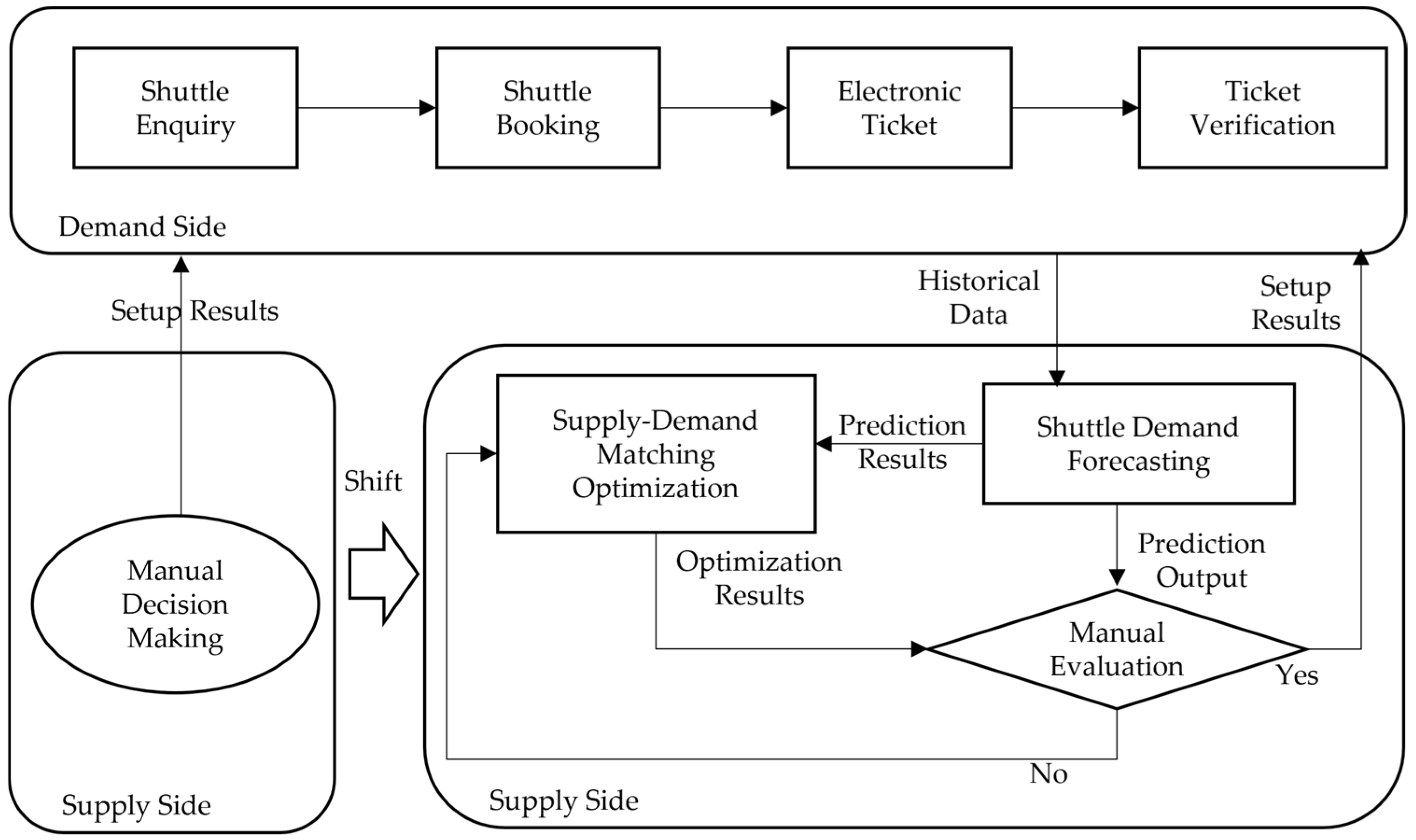
Traditionally, due to limited shuttle resources and the unpredictable demand, the supply side has relied on manual judgement. This study utilizes historical data to develop demand prediction techniques and supply–demand matching model for prediction and optimization. This approach facilitates a strategic transition in shuttle resource allocation from manual decision-making to quantitative decision-making. The demand-side process is passenger-centric through standardized online services, including shuttle inquiry, reservation, electronic ticketing, and boarding verification. This process provides historical data to support quantitative decision-making.

The supply-side quantitative decision-making system adopts a hybrid decision-making mode of data-driven and human–machine collaboration. It includes three layers: prediction, optimization, and evaluation. Among them, the prediction layer adopts the shuttle demand prediction model established in Section 3.1 of this paper, the optimization layer adopts the supply–demand matching method in Section 3.2, and the evaluation layer uses two core indicators to evaluate supply–demand matching effect including resource utilization rate ${\mathrm{z}}_1$ and demand satisfaction rate ${\mathrm{z}}_2$.

As shown in Figure 1, the quantitative decision-making system for shuttle resource allocation utilizes a three-layer decision-making framework consisting of prediction, optimization, and evaluation. The prediction layer leverages historical data and utilizes trained shuttle demand prediction model to generate quantitative results, thereby providing a data-driven baseline for resource allocation. The optimization layer takes the prediction results as input and utilizes a supply–demand matching optimization model to compute the optimal allocation between shuttle supply and demand, thereby generating a preliminary shuttle allocation optimization. The evaluation layer adopts two core indicators, namely resource utilization rate (${\mathrm{z}}_1$) and demand satisfaction rate (${\mathrm{z}}_2$) to evaluate the supply–demand matching effect of shuttle resources. If the evaluation indicators of the optimization resource allocation meet the predefined performance criteria, they will be directly used as the final shift allocation. Otherwise, the result will be returned to the supply–demand matching and optimization model for re-iteration until a feasible resource allocation is obtained. The quantitative decision-making system for shuttle resource allocation can also be simplified into a two-layer system consisting of prediction and evaluation. In this framework, the prediction layer outputs predicting results, and the evaluation layer adopts two core indicators to evaluate the supply–demand matching effect of the manual shift resource allocation based on the prediction results. If the evaluation indicators of the allocation are satisfactory, the manual allocation results are exported as shift ticket set volume; otherwise, manual adjustment is performed again until a feasible allocation is obtained.

4. Results

4.1. Results of Shuttle Demand Prediction Based on Ensemble Learning

• Dataset Construction

This study utilizes student shuttle reservation dataset from a semester at a certain University as the research object. The raw data consists of three primary data tables, the details of which are as follows:

• Basic shuttle table contains 3212 rows including columns of shuttle ID, departure place, departure date, departure time, destination, date type, bus route, ticket set volume and update time.
• Reservation table contains 27,733 rows including columns of reservation ID, student ID, shuttle ID, departure date, departure place, destination, route, departure date, departure time, and ticket status.
• Search log table contains 188,044 rows including columns of search ID, student ID, name, departure place, destination, departure date, departure time, shuttle ID and update time.

The primary dataset was built by adding Reservation Demand column and Search Volume column to the Basic shuttle table. For each unique shift (defined by its departure place, destination, departure date and departure time), we counted its occurrences in both the reservation and search log tables. These counts were then filled into the corresponding rows of the basic table.

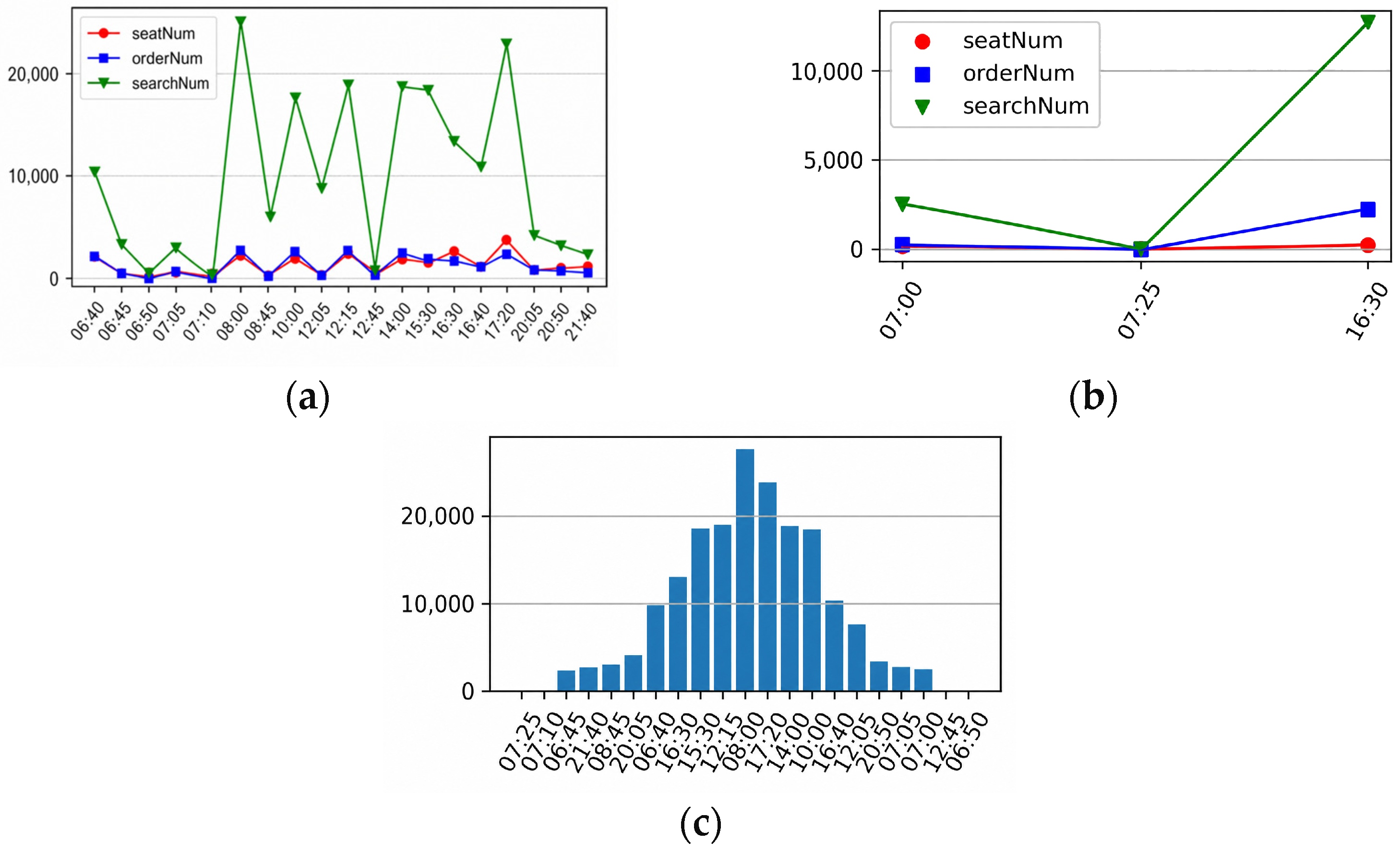
Figure 2a and Figure 2b illustrate the shift popularity on weekdays and weekends, respectively. The x-axis lists departure times in chronological order, consisting of 19 weekday shifts and 3 weekend shifts. The y-axis represents the total quantity of each category. Specifically, red circles denote the total number of bookable seats for each shift during this semester. Blue rectangles indicate the total volume of tickets actually booked, while green triangles represent the total number of searches performed for each shift. In the shift intensity analysis, three shifts (16:30, 17:20, and 21:40) show a higher number of seats than actual reservation, indicating that supply exceeds demand. In these cases, the seat capacity can be reduced based on the demand prediction. Conversely, for the other 16 shifts, the number of reservations is equal to or greater than the available seats, suggesting that demand exceeds supply. For these shifts, the seat capacity could be increased according to the prediction results. Figure 2c displays the search volume for each shift where the x-axis lists shuttle shifts, and the y-axis represents the total search frequency. In this visualization, shifts are arranged in descending order, radiating from the center toward both sides. The resulting curve exhibits a bell shape that closely follows a normal distribution, characterized by a central peak tapering off as it nears the x-axis. Out of 188,044 searches, a mere 50% of shifts captured 91.7% of user interest. These findings suggest that optimizing departure time and ticket allocation for these specific shifts is critical for achieving better supply and demand alignment.

2.

Feature Engineering

Based on the dataset, a prediction sample dataset consisting of 13 columns and 3212 rows was constructed using feature engineering methods. This includes 12 feature columns plus one target variable column. The statistical characteristics of these 13 data items are summarized in the

Table 1. Statistical information of the model dataset.

Column	Na_Ratio	Type	Mean	Std	Min	25%	50%	75%	Max
year	0.0	int64	2024.0025	0.049844	2024	2024	2024	2024	2025
month	0.0	int64	9.7665	2.7782	1	9	10	11	12
day	0.0	int64	15.5953	8.7298	1	9	15	23	31
hour	0.0	int64	12.5872	4.4057	6	8	12	16	21
minute	0.0	int64	21.6283	16.8052	0.0	5	20	40	50
weekday	0.0	int64	3.2491	1.6119	1	2	3	5	7
weekofyear	0.0	int64	39.8493	13.573	1	38	43	48	52
daytype	0.0	int64	1.0672	0.3203	1	1	1	1	3
start	0.0	int64	1.9835	1.026	1	1	2	2	5
end	0.0	int64	1.8677	0.9252	1	1	2	2	5
ticketNum	0.0	int64	9.9328	6.614	0.0	5	10	15	25
searchNum	0.0	int64	69.2375	84.2402	0.0	1	46.5	101	724
orderNum	0.0	int64	9.637	9.0555	0.0	0.0	9	17	33

.

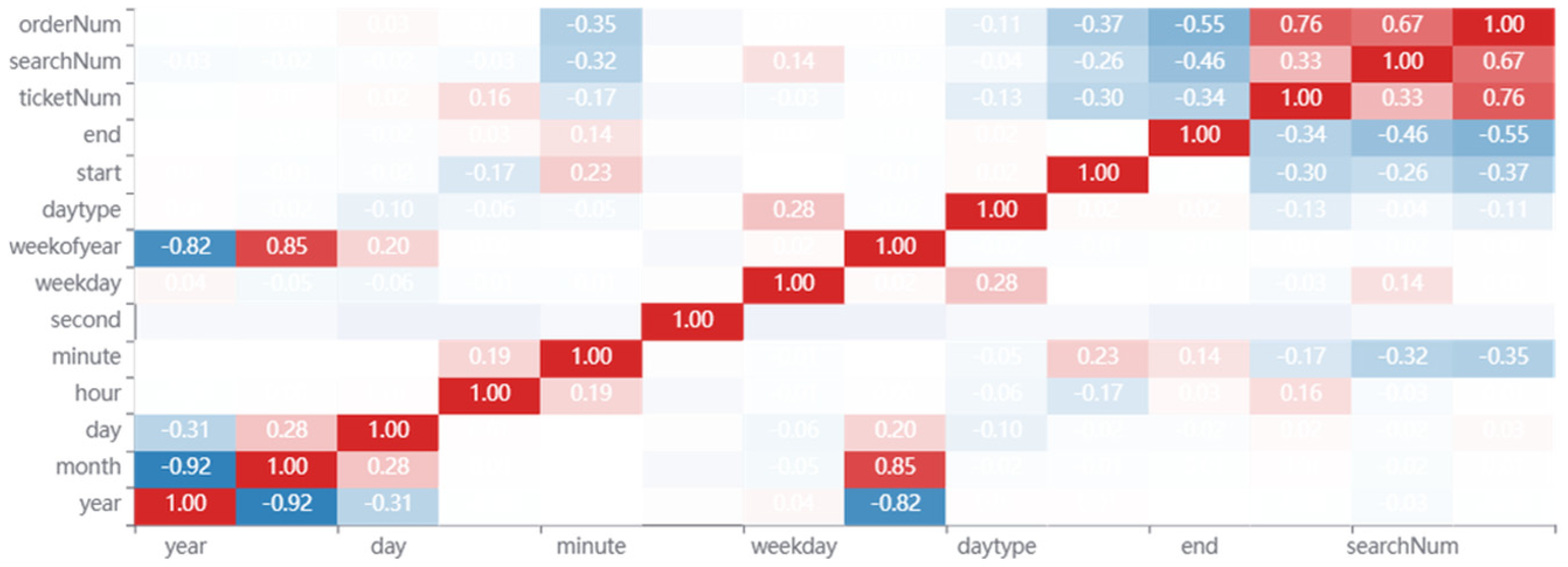
Following the Pearson correlation analysis, a heat map of the correlation matrix for all variables in the sample dataset was computed and visualized, as shown in Figure 3. The heat map illustrates the degree of linear correlation between different variables through color intensity: deeper red denotes a stronger positive correlation (coefficient approaching 1), deeper blue indicates a stronger negative correlation (coefficient approaching −1), and white represents a negligible or extremely weak correlation (coefficient approaching 0).

Several key findings can be derived from the correlation matrix heat map:

• Key Features: The ticket reservation volume (orderNum) is strongly and positively correlated with search volume (searchNum) and ticket set volume (ticketNum), with correlation coefficients of 0.67 and 0.76, respectively. This aligns with the underlying actual scenario: an increase in user search volume drives reservation volume, which in turn reflects the growth in reservation volume. These findings suggest that searchNum and ticketNum are critical features for orderNum.
• Feature Elimination: The feature weekofyear shows strong correlations with month and year (correlation coefficients of 0.85 and −0.82, respectively), indicating significant feature redundancy. To enhance prediction model precision, the month and year features were removed, reducing the sample dataset to a more efficient 11 columns.

3.

Prediction Model Construction and Performance Evaluation

• Training Set Partitioning

The feature-engineered dataset was partitioned into training (80%) and test (20%) sets. consisting of 2569 rows and 11 columns, while the test dataset contains 643 rows and 11 columns.

• Comparison Analysis of Five Machine Learning Algorithms

According to the hyperparameter configurations of the 5 machine learning algorithms shown in Appendix A, prediction models were trained on the training set using five distinct machine learning algorithms: LGB, RF, XGB, SVR, and MLP. Upon completion of the model training phase, predictions were executed on test dataset. Seven evaluation metrics were designed based on the previously proposed evaluation methodology to assess the model’s performance. The metrics are listed in the

Table 2. Evaluation results of five machine learning algorithms on the test set.

	R2	RMSE	MSE	MAE	Hit_Rate_1	Hit_Rate_2	Hit_Rate_3
LGB	0.9635	1.7227	2.9675	1.1214	58.79	81.03	91.91
RF	0.9645	1.6986	2.8854	1.0857	60.34	80.87	91.14
XGB	0.9625	1.7455	3.0467	1.2014	57.54	78.23	91.29
SVR	0.8797	3.1272	9.7791	2.0287	45.26	63.45	75.43
MLP	0.9439	2.1361	4.5630	1.4678	52.72	73.72	86.31

.

For the evaluation metrics, higher scores in R² and hit rates (hit_rat_1, hit_rate_2, and hit_rate_3) and lower scores in error in RMSE, MSE, and MAE signify superior model accuracy. Based on the evaluation results from the test dataset, the ensemble tree-based models—represented by LGB, RF, and XGB—demonstrated superior performance. Specifically, RF achieved the highest precision across regression metrics (R², RMSE, MSE, and MAE). Meanwhile, LGB exhibited the best performance in terms of hit rates (hit_rat_1, hit_rate_2, and hit_rate_3) and maintained the highest overall stability. The MLP model followed in performance, while SVR performed significantly worse than the other candidate models.

While testing set metrics reflect prediction accuracy, the performance discrepancy between the training and test sets serves as a direct metric of the model’s generalization ability. A significant performance gap where the training set outperforms the test set indicates overfitting, suggesting poor adaptability to unseen data. Conversely, a minimal gap demonstrates strong model stability and superior generalization ability, making the model more suitable for practical applications. To provide a comprehensive assessment of model robustness, the performance differences between the training and test sets are further compared in

Table 3. Evaluation results between the training and test sets for five machine learning algorithms.

		R2	RMSE	MSE	MAE	Hit_Rate_1	Hit_Rate_2	Hit_Rate_3
LGB	test	0.9635	1.7227	2.9675	1.1214	58.79	81.03	91.91
	train	0.9746	1.4441	2.0855	0.9243	66.41	86.10	95.25
RF	test	0.9645	1.6986	2.8854	1.0857	60.34	80.87	91.14
	train	0.9935	0.7314	0.5349	0.4239	88.17	97.43	99.46
XGB	test	0.9625	1.7455	3.0467	1.2014	57.54	78.23	91.29
	train	0.9595	1.8247	3.3295	1.2146	58.08	78.82	89.84
SVR	test	0.8797	3.1272	9.7791	2.0287	45.26	63.45	75.43
	train	0.9036	2.8138	7.9175	1.7802	50.64	67.54	79.80
MLP	test	0.9439	2.1361	4.5630	1.4678	52.72	73.72	86.31
	train	0.9409	2.2025	4.8512	1.4330	53.99	75.87	87.12

below.

The following sections provide a detailed analysis of the experimental results based on regression accuracy metrics (R², RMSE, MSE, and MAE) and hit rate metrics (hit_rate_1, hit_rate_2, hit_rate_3).

• Evaluation of Regression Performance

RF achieves the highest training R² (0.9935) and lowest RMSE (0.7314), but exhibits clear overfitting due to the large gap between training and test sets. LGB demonstrates the best generalization, with a test R² of 0.9635 and RMSE of 1.7227, showing the most consistent performance. XGB performs slightly below LGB and RF, with the R2 value on the training set is lower than that on the test set. SVR shows the poorest results across all metrics, while MLP maintains a moderate performance level between LGB, XGB and SVR.

• Analysis of Hit Rate

RF has a high hit rate on the training dataset (hit_rate_3 = 99.46%), but the test dataset is only 91.14%, indicating clear overfitting. LGB achieved a hit_rate_3 of 91.91% on the test dataset, which is the highest among all models. It also shows the smallest gap between the training and test datasets, demonstrating the best stability. The hit rates for XGB and MLP are moderate; XGB’s hit_rate_2 (78.23%) is slightly lower than those of LGB and RF. SVR has the lowest hit rate (hit_rate_3 = 75.43%), which is consistent with its performance across regression metrics.

LGB demonstrates the best comprehensive performance with strong generalization capabilities. Its regression metrics and hit rates on the test dataset are both among the top layer, showing no significant overfitting. While RF shows near-perfect results on the training set while suffers from severe overfitting. SVR exhibits the poorest performance and is unsuitable for this task.

While the comparative analysis of evaluation metrics reveals that the LGB model excels in hit rate and overall stability, statistical significance tests were further conducted to rigorously validate these performance gaps. The results of the Wilcoxon Signed-Rank Test [34] confirm that the superior performance of the LGB model is statistically significant across the test suite. Specifically, the p-values for LGB compared to RF and XGB are 4.47 × 10⁻³ and 2.55 × 10⁻⁴ respectively, both falling well below the critical threshold of 0.05. Even more substantial differences are observed when comparing LGB to the MLP (p = 3.13 × 10⁻¹⁴) and SVR models (p = 7.90 × 10⁻²³). These statistical results provide robust evidence that the LGB model’s advantage, particularly its balance of high hit rates and predictive stability, is consistent and reliable rather than a result of stochastic variation.

• Performance Enhancement based on Ensemble Learning

To further improve prediction performance, a bagging ensemble strategy was applied to the five base models described above. Specifically, a bootstrap sampling technique (sampling with replacement) was employed to train 10 individual base learners for each model. The final predictions for the five resulting ensemble models were obtained by averaging the outputs of these learners. The evaluation results are summarized in

Table 4. Evaluation results for five machine learning algorithms before and after ensemble learning.

	R2	RMSE	MSE	MAE	Hit_Rate_1	Hit_Rate_2	Hit_Rate_3
LGB	0.9635	1.7227	2.9675	1.1214	58.79	81.03	91.91
LGB_bagging	0.9658	1.6663	2.7765	1.0838	60.65	81.18	92.22
RF	0.9645	1.6986	2.8854	1.0857	60.34	80.87	91.14
RF_bagging	0.9667	1.6461	2.7096	1.0436	61.43	81.65	92.38
XGB	0.9625	1.7455	3.0467	1.2014	57.54	78.23	91.29
XGB_bagging	0.9612	1.7757	3.1530	1.1996	59.25	77.76	89.89
SVR	0.8797	3.1272	9.7791	2.0287	45.26	63.45	75.43
SVR_bagging	0.8776	3.1545	9.9507	2.0641	45.41	62.67	74.34
MLP	0.9439	2.1361	4.5630	1.4678	52.72	73.72	86.31
MLP_bagging	0.9517	1.9804	3.9218	1.3921	53.34	74.81	87.40

below.

As shown by the evaluation results on the test set, the Bagging ensemble strategy significantly enhances model performance. With the exception of slight fluctuations in XGB and SVR, LGB, RF and MLP models all show comprehensive improvements after applying Bagging. Specifically, these models yield higher R² values and lower RMSE, MSE, and MAE, alongside an overall improvement across all hit rate metrics.

The evaluation metrics on the test set reflect the prediction accuracy of the models, while the gap between training and test performance directly characterizes their generalization ability and degree of overfitting. To comprehensively evaluate model performance, a comparison of the results across both sets is presented in

Table 5. Evaluation results between the training and test sets for five ensemble-based ML algorithms.

		R2	RMSE	MSE	MAE	Hit_Rate_1	Hit_Rate_2	Hit_Rate_3
LGB_ bagging	test	0.9658 *	1.6663 *	2.7765 *	1.0838 *	60.65 *	81.18 *	92.22 *
	train	0.9730	1.4882	2.2148	0.9349	66.95	86.69	94.82
RF_ bagging	test	0.9667 *	1.6461 *	2.7096 *	1.0436 *	61.43 *	81.65 *	92.38 *
	train	0.9835	1.1627	1.3518	0.6823	75.48	92.10	96.81
XGB_ bagging	test	0.9612 *	1.7757 *	3.1530 *	1.1996 *	59.25 *	77.76 *	89.89 *
	train	0.9589	1.8372	3.3753	1.2243	58.51	77.97	90.00
SVR_ bagging	test	0.8776 *	3.1545 *	9.9507 *	2.0641 *	45.41 *	62.67 *	74.34 *
	train	0.9036	2.8134	7.9155	1.8025	50.18	67.11	79.49
MLP_ bagging	test	0.9517 *	1.9804 *	3.9218 *	1.3921 *	53.34 *	74.81 *	87.40 *
	train	0.9400	2.2199	4.9281	1.4293	53.80	75.83	87.08

Values marked with an asterisk (*) and shown in italics represent the performance metrics on the test set; non-italicized values represent the performance metrics on the training set.

.

The analysis indicates that although RF_bagging achieves the best regression metrics and hit rates on the test dataset, it exhibits a significant performance gap between the training and test sets. For instance, R² decreases from 0.9835 to 0.9667 and hit_rate_1 drops from 75.48% to 61.43%, suggesting obvious overfitting and limited generalization. In contrast, LGB_bagging demonstrates test dataset accuracy comparable to RF_bagging while maintaining the smallest gap between training and testing performance. This confirms the absence of significant overfitting and proves that LGB_bagging offers the best generalization and stability. The performance of XGB_bagging and MLP_bagging is moderate, while SVR_bagging remained significantly inferior to the other ensemble models across all evaluated indicators.

The Wilcoxon Signed-Rank Test was further employed to rigorously assess the statistical significance of the performance improvements. Taking LGB_bagging as the reference model, the results indicate that it significantly outperforms all other candidates across the test suite. Specifically, the p-values obtained from the pairwise comparisons between LGB_bagging and its counterparts, RF_bagging (p = 3.14 × 10⁻⁴), XGB_bagging (p = 1.70 × 10⁻⁶), SVR_bagging (p = 5.75 × 10⁻²⁸), and MLP_bagging (p = 5.75 × 10⁻²⁸) are all substantially lower than the 0.01 significance threshold. These statistical findings provide conclusive evidence that the superior generalization and stability of LGB_bagging are not only numerically evident but also statistically robust, distinguishing it as the most reliable model for this application.

Consequently, by balancing prediction accuracy and generalization capability, LGB_bagging is identified as the optimal candidate for the final prediction model in this study.

4.2. Results of Supply–Demand Matching Results Based on Multi-Objective Optimization

• Supply–Demand Matching Model and Solution Based on multi-objective optimization

We next take a certain shuttle allocation as an example to verify the multi-objective optimization model for the supply–demand matching of shuttle resources and its solution method for the Pareto optimal set.

(1)

Due to the limited shuttle resources, a certain allocation is designated as

$\mathrm{ticketNum}\_\mathrm{set}\in \left[10,19\right]=[\min ,\max ].$

(2)

For $\forall \mathrm{ticketNum}\_\mathrm{set}\in \left[\min ,\max \right]$, a complete dataset of shift information is constructed. A single-factor sensitivity analysis is adopted, where all shift information remains unchanged except for the decision variable $\mathrm{ticketNum}\_\mathrm{set}$. Based on the feature engineering results in Section 4.1, a total of 10 feature variables are identified: day, hour, minute, weekday, weekofyear, daytype, start, end, ticketNum, searchNum, and orderNum. The complete shift feature dataset is denoted as below:

$$\mathrm{X}\_\mathrm{set}(\mathrm{ticketNum}\_\mathrm{set})$$

(17)

(3)

Based on the well-trained shuttle demand prediction model LGB_bagging, for $\forall \mathrm{ticketNum}\_\mathrm{set}\in \left[\min ,\max \right]$, $\mathrm{orderNum}\_\mathrm{predict}$ can be computed:

$$\mathrm{orderNum}\_\mathrm{predict}=\mathrm{LGB}\_\mathrm{bagging}(\mathrm{X}\_\mathrm{set}(\mathrm{ticketNum}\_\mathrm{set})),$$

(18)

$\mathrm{ticketNum}\_\mathrm{set}$, $\mathrm{orderNum}\_\mathrm{predict}$, and $\mathrm{orderNum}\_\mathrm{predict}-\mathrm{ticketNum}\_\mathrm{set}$ are shown in the table below.

(4)

Observing the third column of the table above, according to Theorem A1,

$\exists \mathrm{ticketNum}\_\mathrm{set}=16\in [\min ,\max ]$, satisfying,

$\mathrm{orderNum}\_\mathrm{predict}-\mathrm{ticketNum}\_\mathrm{set}=16-16=0$

Then the Pareto optimal solution set of the shuttle bus resource supply–demand matching optimization model is:

$$\left\{\mathrm{ticketNum}\_\mathrm{set}\left|\mathrm{orderNum}-\mathrm{ticketNum}=0\right.\right\}=\left\{16\right\}.$$

When $\mathrm{ticketNum}\_\mathrm{set}=16$, resource utilization rate ${\mathrm{z}}_1$ and demand satisfaction rate ${\mathrm{z}}_2$ are respectively:

$${\mathrm{z}}_1={\displaystyle \frac{\min \left\{\mathrm{ticketNum}\_\mathrm{set},\mathrm{orderNum}\_\mathrm{predict}\right\}}{\mathrm{ticketNum}\_\mathrm{set}}}\times 100={\displaystyle \frac{\min \{16,16\}}{16}}\times 100=100\%,$$

$${\mathrm{z}}_2={\displaystyle \frac{\min \left\{\mathrm{ticketNum}\_\mathrm{set},\mathrm{orderNum}\_\mathrm{predict}\right\}}{\mathrm{orderNum}\_\mathrm{predict}}}\times 100={\displaystyle \frac{\min \left\{16,16\right\}}{16}}\times 100=100\%.$$

That is, the maximum values are achieved on both objectives, and the Pareto optimal solution set obtained by Theorem A1 can achieve the optimal supply–demand matching of shuttle resources. Thus, Theorem A1 is verified.

To further verify Theorem A2, we set $\mathrm{orderNum}\_\mathrm{predict}(16)=17$, then:

$$\mathrm{orderNum}\_\mathrm{predict}-\mathrm{ticketNum}\_\mathrm{set}=17-16=1$$

Based on

Table 6. Single-factor sensitivity analysis table for ticket set volume.

TicketNum_Set	OrderNum_Predict	OrderNum_Predict−TicketNum_Set
10	6	−4
11	6	−5
12	6	−6
13	16	3
14	16	2
15	16	1
16	16	0
17	16	−1
18	16	−2
19	16	−3

, we updated the above two values, then we got

Table 7. Updated Single-factor sensitivity analysis table for ticket set volume.

TicketNum_Set	OrderNum_Predict	OrderNum_Predict−TicketNum_Set
10	6	−4
11	6	−5
12	6	−6
13	16	3
14	16	2
15	16	1
16	17	1
17	16	−1
18	16	−2
19	16	−3

as below.

Observing the third column of the above table, according to item (3) of Theorem A2, the Pareto optimal solution set of the shuttle bus resource supply–demand matching optimization model is:

$$\begin{gathered} \left\{\arg {\max }_{\mathrm{ticketNum}\_\mathrm{set}}\{{\displaystyle \frac{\mathrm{orderNum}\_\mathrm{predict}}{\mathrm{ticketNum}\_\mathrm{set}}}\left|\mathrm{orderNum}\_\mathrm{predict}-\mathrm{ticketNum}\_\mathrm{set}<0\right.\}\right\}\cup \\ \left\{\arg {\max }_{\mathrm{ticketNum}\_\mathrm{set}}\{{\displaystyle \frac{\mathrm{ticketNum}\_\mathrm{set}}{\mathrm{orderNum}\_\mathrm{predict}}}\left|\mathrm{orderNum}\_\mathrm{predict}-\mathrm{ticketNum}\_\mathrm{set}>0\right.\}\right\} \\ =\left\{\arg {\max }_{\mathrm{ticketNum}\_\mathrm{set}}\{{\displaystyle \frac{6}{10}},{\displaystyle \frac{6}{11}},{\displaystyle \frac{6}{12}},{\displaystyle \frac{16}{17}},{\displaystyle \frac{16}{18}},{\displaystyle \frac{16}{19}}\}\right\}\cup \left\{\arg {\max }_{\mathrm{ticketNum}\_\mathrm{set}}\{{\displaystyle \frac{13}{16}},{\displaystyle \frac{14}{16}},{\displaystyle \frac{15}{16}},{\displaystyle \frac{16}{17}}\}\right\} \\ =\left\{17\right\}\cup \left\{16\right\}=\left\{16,17\right\} \end{gathered}$$

When $\mathrm{ticketNum}\_\mathrm{set}=16$, resource utilization rate ${\mathrm{z}}_1$ and demand satisfaction rate ${\mathrm{z}}_2$ are respectively:

$${\mathrm{z}}_1={\displaystyle \frac{\min \left\{\mathrm{ticketNum}\_\mathrm{set},\mathrm{orderNum}\_\mathrm{predict}\right\}}{\mathrm{ticketNum}\_\mathrm{set}}}\times 100={\displaystyle \frac{\min \{16,17\}}{17}}\times 100=94\%,$$

$${\mathrm{z}}_2={\displaystyle \frac{\min \left\{\mathrm{ticketNum}\_\mathrm{set},\mathrm{orderNum}\_\mathrm{predict}\right\}}{\mathrm{orderNum}\_\mathrm{predict}}}\times 100={\displaystyle \frac{\min \left\{16,17\right\}}{16}}\times 100=100\%,$$

When $\mathrm{ticketNum}\_\mathrm{set}=17$, resource utilization rate ${\mathrm{z}}_1$ and demand satisfaction rate ${\mathrm{z}}_2$ are respectively:

$${\mathrm{z}}_1={\displaystyle \frac{\min \left\{\mathrm{ticketNum}\_\mathrm{set},\mathrm{orderNum}\_\mathrm{predict}\right\}}{\mathrm{ticketNum}\_\mathrm{set}}}\times 100={\displaystyle \frac{\min \{17,16\}}{17}}\times 100=94\%,$$

$${\mathrm{z}}_2={\displaystyle \frac{\min \left\{\mathrm{ticketNum}\_\mathrm{set},\mathrm{orderNum}\_\mathrm{predict}\right\}}{\mathrm{orderNum}\_\mathrm{predict}}}\times 100={\displaystyle \frac{\min \left\{17,16\right\}}{16}}\times 100=100\%$$

It is easy to see that both $\mathrm{ticketNum}\_\mathrm{set}=16$ and $\mathrm{ticketNum}\_\mathrm{set}=17$, are non-dominated solutions and do not dominate each other, and $\left\{16,17\right\}$ constitutes the Pareto optimal solution set of the shuttle bus resource supply–demand matching optimization model. Thus, Theorem A2 is verified.

2.

Quantitative Decision-making Process for Shuttle Resource Allocation

Based on the shuttle demand prediction and supply–demand matching optimization models proposed in this paper, the quantitative decision-making framework can transform shuttle resource allocation from manual experience-based decision-making to quantitative decision-making. Taking the shift information in the case of Section 4.2 as an example, the prediction-optimization-evaluation three-layer framework and the prediction-evaluation two-layer framework are illustrated, respectively.

• Quantitative Decision-Making Process Based on the Prediction-Optimization-Evaluation Three-Layer Framework

For the shift ticket volume set by manual experience decision-making:

$\mathrm{ticketNum}\_\mathrm{set}=15$, after processing by the shuttle demand prediction and supply–demand matching optimization model, the optimal supply–demand matching result is obtained as $\mathrm{ticketNum}\_\mathrm{set}=16$. The result is then passed to the manual evaluation process. Based on the shuttle resource allocation status shown in Table 7, the resource utilization rate ${\mathrm{z}}_1$ and demand satisfaction rate ${\mathrm{z}}_2$ are calculated and presented in

Table 8. Quantitative decision evaluation table for shuttle resource allocation.

TicketNum_Set	OrderNum_Predict	OrderNum_Predict − TicketNum_Set	${\mathbf{z}}_{\mathbf{1}}\mathbf{,}\mathbf{\%}$	${\mathbf{z}}_{\mathbf{2}}\mathbf{,}\mathbf{\%}$
10	6	−4	60	100
11	6	−5	55	100
12	6	−6	50	100
13	16	3	100	81
14	16	2	100	88
15	16	1	100	94
16	16	0	100	100
17	16	−1	94	100
18	16	−2	89	100
19	16	−3	84	100

.

When $\mathrm{ticketNum}\_\mathrm{set}\ge 16$ or $\mathrm{ticketNum}\_\mathrm{set}\le 12$, the resource utilization rate ${\mathrm{z}}_1<100\%$, resulting in waste of shift resources.

When $\mathrm{ticketNum}\_\mathrm{set}\in \left[13,16\right]$, the resource utilization rate ${\mathrm{z}}_1=100\%$, reaching its maximum. Specifically, when $\mathrm{ticketNum}\_\mathrm{set}=16$, the resource utilization rate ${\mathrm{z}}_1=100\%$ and the demand satisfaction rate ${\mathrm{z}}_2=100\%$. A manual evaluation of the supply–demand matching effect of shuttle resources is conducted: both the resource utilization rate and demand satisfaction rate reach their maximum, indicating that this resources allocation achieves the optimal matching of shuttle supply and demand, and can be issued to the demand side as the final shuttle resource allocation.

2.

Quantitative Decision-Making Process Based on the Prediction-Evaluation Two-Layer System

For the shift ticket set volume by manual decision-making: $\mathrm{ticketNum}\_\mathrm{set}=15$, after processing by the shuttle demand prediction, the predicted ticket reservation volume is obtained: $\mathrm{orderNum}\_\mathrm{predict}=16$. The resource utilization rate ${\mathrm{z}}_1$ and demand satisfaction rate ${\mathrm{z}}_2$ of this allocation are calculated, yielding ${\mathrm{z}}_1=100\%$, ${\mathrm{z}}_2=94\%$. A manual evaluation of the supply–demand matching effect of shuttle resources is conducted: the resource utilization rate has reached its maximum, while the demand satisfaction rate needs to be improved.

The manual adjustment for the shift ticket set volume is continued:

$\mathrm{ticketNum}\_\mathrm{set}=14$. After processing by the shuttle demand prediction model, the predicted ticket reservation volume is obtained as $\mathrm{orderNum}\_\mathrm{predict}=16$. The resource utilization rate ${\mathrm{z}}_1$ and demand satisfaction rate ${\mathrm{z}}_2$ of this allocation are calculated, yielding ${\mathrm{z}}_1=100\%$, ${\mathrm{z}}_2=88\%$. A manual evaluation of the supply–demand matching effect of shuttle resources is conducted: the resource utilization rate has reached its maximum, while the demand satisfaction rate still needs to be improved.

The manual adjustment for the ticket set volume is continued: $\mathrm{ticketNum}\_\mathrm{set}=16$. After processing by the shuttle demand prediction model, the predicted ticket reservation volume is obtained as $\mathrm{orderNum}\_\mathrm{predict}=16$. The resource utilization rate ${\mathrm{z}}_1$ and demand satisfaction rate ${\mathrm{z}}_2$ of this scheme are calculated, yielding ${\mathrm{z}}_1=100\%$, ${\mathrm{z}}_2=100\%$. A manual evaluation of the supply–demand matching effect of shuttle resources is conducted: Both the resource utilization rate and the demand satisfaction rate reach their maximum, enabling the optimal supply–demand matching of shuttle resources. This result can provide to the demand side as the final shuttle resource allocation.

5. Discussion

Aiming at the core challenges of “uncertain demand, limited resources, and supply–demand mismatching” in university shuttle services, this paper systematically discusses and in-depth interprets the case verification results by integrating relevant research achievements in the fields of previous university data mining, university resource allocation, and public transit resource allocation, as well as the research hypotheses proposed in this paper regarding university shuttle demand forecasting and supply–demand matching optimization. Firstly, by comparing the differences between the proposed “ensemble learning + multi-objective optimization” method and existing research methods, this study clarifies the alignment points and innovations: previous studies on university resource allocation mostly focused on resource recommendation, and the methods for public transport resource allocation are difficult to be directly transferred to the university shuttle scenario. In contrast, this paper focuses on the micro-scenario of university shuttle resource allocation, constructs a three-layers decision-making system of “prediction-optimization-evaluation”, makes up for the deficiencies of existing research in the field of shuttle resource optimization, and promotes the transformation of shuttle resource allocation from experience-based decision-making to quantitative decision-making.

Combined with the case verification results, this paper in-depth interprets the core value of the research findings: the study confirms that searchNum (search volume), ticketNum (ticket quantity), and orderNum (ticket reservation volume) of shuttle buses show a strong positive correlation (correlation coefficients 0.67 and 0.76), which can be used as key features for shuttle bus demand prediction. This finding provides a clear basis for feature selection in subsequent university shuttle bus demand prediction and solves the problem of blindness in feature selection of previous prediction models. In the comparison of prediction models, single models have obvious shortcomings: RF performs the best on the training set (R² = 0.9935, RMSE = 0.7314) but has serious overfitting, SVR performs the worst, and MLP and XGB have moderate performance. However, the Bagging ensemble strategy effectively improves the model performance. Among them, LGB_bagging not only has a test set accuracy close to that of RF_bagging, but also has the smallest difference between the training set and the test set, no obvious overfitting, and the optimal generalization ability and stability. This result verifies the effectiveness of ensemble learning in shuttle bus demand prediction and also provides a reference for the selection of prediction models in similar scenarios.

In the verification of the multi-objective optimization model, the effectiveness of the proposed solution method and theorems is confirmed through two cases: Theorem A1 verifies that when the set value of the ticket quantity in the decision space is equal to the predicted value of the ticket reservation volume, this set value is a Pareto optimal solution; Theorem A2 clarifies the impact of the ratio between the set value of the ticket quantity and the predicted value of ticket reservation volume on the value of the objective function, provides theoretical support for the rapid solution of the Pareto optimal solution set, and solves the problems of single optimization objective and low solution efficiency in previous shuttle bus supply–demand matching.

5.1. Generalization Analysis of the Research Method

Although this study focuses on the specific scenario of university shuttle buses and the group of teachers and students, the proposed method has strong generalization ability and can be adapted to different settings and a wider range of user groups. From the perspective of method logic, the core framework of “ensemble learning prediction—multi-objective optimization—three-layer decision-making system” is not limited to the university scenario; its essence is a closed-loop idea of “demand quantification-resource optimization-decision implementation”, which can be applied to similar commuting service scenarios through scenario adaptation and adjustment. Specifically, for internal corporate commuter shuttle buses, the prediction features can be replaced with employee attendance data, etc., and the optimization objectives can be adjusted (such as focusing on corporate operating cost control) to achieve method migration; for primary and secondary school commuter shuttle buses, features such as students’ school arrival and departure times and parents’ pick-up and drop-off needs can be integrated, and the model constraints can be optimized (such as increasing safety priority) to adapt to the special needs of minors’ commuting; for university resource allocation, this method can be extended to other public service resource fields in universities, such as campus shuttle buses, shared laboratory resources, and library lending resources. The prediction features can be replaced with students’ campus activity trajectories, laboratory reservation data, book lending records, etc., the core objectives of the multi-objective optimization model can be adjusted (such as balancing resource utilization and the convenience of teachers and students), and the three-layer decision-making system of “prediction-optimization-evaluation” can be used to achieve accurate allocation of various public service resources in universities, solve the common problems of mismatched supply and demand and low utilization rate of university resources, further extend the application value of the research method in the university field, and provide more comprehensive technical support for data-driven resource governance in universities.

5.2. Policy Recommendations and Practical Significance of the Research

This study not only has clear theoretical value, but also can provide practical support for the operation and management of university shuttle buses and the formulation of relevant policies. The specific policy recommendations and practical significance are as follows:

In terms of policy recommendations: first, it is recommended that university logistics management departments establish a “data-driven” shuttle operation and management mechanism, integrate the “prediction-optimization-evaluation” making system proposed in this paper into the daily scheduling system, formulate standardized shuttle resource allocation processes, replace traditional experience-based manual decision-making, and improve the level of operational standardization; second, it is recommended that education authorities incorporate intelligent scheduling of university shuttle buses into the relevant policy orientation for improving the quality and efficiency of university logistics services, encourage universities to strengthen the integration and sharing of campus commuting data, promote the coordinated optimization of cross-university shuttle resources, and reduce the commuting operation costs of regional universities.

In terms of practical significance, from the perspective of universities, the method proposed in this paper helps solve the problem of supply–demand mismatch of university shuttle buses, such as overcrowding during peak hours and resource idleness during off-peak hours, improve the utilization rate of shuttle resources and the demand satisfaction rate of teachers and students, reduce the waiting time of teachers and students, improve the commuting experience, and further enhance the quality of university logistics services. From the industry perspective, the three-layer decision-making system of “prediction-optimization-evaluation” constructed in this paper provides a referenceable solution for the allocation of similar commuting services (such as corporate commuting and park commuting) and university resource allocation, and promotes the transformation of commuting services from experience-based management to intelligent and quantitative management. From the theoretical perspective, it enriches the research achievements in the fields of university data mining and resource allocation, makes up for the deficiencies of existing research in the field of shuttle resource allocation, and provides method reference and theoretical support for subsequent related research.

5.3. Limitations of the Research

Although this study has achieved the expected results in university shuttle bus demand prediction and supply–demand matching optimization, and the proposed method has strong generalization ability, it still has certain limitations that need to be further improved in subsequent research. First, there are limitations in the data dimension. The prediction model in the current study mainly relies on basic data such as shuttle bus search and reservation data, and does not fully integrate dynamic data such as students’ curriculum information, campus activity arrangements, weather changes, and surrounding traffic congestion. This may lead to a decline in prediction accuracy in extreme scenarios (such as severe weather and large-scale campus activities), making it difficult to fully capture the impact of various sudden factors on shuttle bus demand. Second, there are limitations in scenario coverage. This study mainly focuses on the optimal allocation of single-route shuttle bus resources in universities, and does not involve more complex campus commuting scenarios such as multi-route collaborative optimization and cross-campus shuttle bus linkage, leaving room for improvement in the scenario adaptability of the method. Third, there are limitations in model optimization. In the multi-objective optimization model, the resource utilization rate and demand satisfaction rate are not dynamically adjusted according to the operational priorities of different universities, and the impact of uncertain factors in shuttle bus operation (such as vehicle failures) on the implementation of the optimization plan is not fully considered, so the flexibility and robustness of the model need to be further enhanced.

6. Conclusions

Targeting the core pain points of university shuttle buses, namely “uncertain demand, limited resources, and supply–demand mismatch”, this paper conducts research on university shuttle bus demand prediction and supply–demand matching optimization. Through model construction, theoretical derivation and case verification, the following core conclusions are drawn:

Firstly, the key features for shuttle bus demand prediction are clarified. searchNum (search volume), ticketNum (tickets quantity), and orderNum (ticket reservation volume) show a strong positive correlation, which can be used as the core input features of the prediction model, providing important support for improving predicting accuracy. Secondly, the advantages of ensemble learning in shuttle bus demand prediction are verified. The LGB_bagging model has the optimal comprehensive prediction accuracy, generalization ability and stability, and can be used as the optimal model for university shuttle bus demand prediction, effectively solving the problems of overfitting and insufficient generalization ability of single models. Thirdly, the constructed multi-objective optimization model and the solution method for Pareto optimal solutions are effective. The optimal solution set can be quickly obtained through two theorems, realizing the balance between resource utilization rate and demand satisfaction rate. Fourthly, the built three-layer decision-making system of “prediction-optimization-evaluation” can effectively promote the transformation of shuttle bus resource allocation from experience-based manual decision-making to quantitative decision-making, providing a standardized process for the operation and management of university shuttle buses.

At the same time, the method proposed in this paper has strong generalization ability, which can be applied to a wider range of scenarios such as internal corporate commuting, primary and secondary school commuting, and park commuting through scenario adaptation and adjustment, providing a reference for the resource optimization of similar commuting services; the policy recommendations and practical paths proposed in the research can effectively guide the improvement of the operation and management quality and efficiency of university shuttle buses, and promote the development of university logistics services towards intelligence and high efficiency.

The limitations of this study are mainly reflected in two aspects: first, there is still room for expansion in the data dimension. The current prediction model is mainly based on basic data such as search and reservation data, and has not fully integrated dynamic data such as curriculum information, weather, and traffic congestion; second, the scenario application is still relatively single, focusing mainly on the optimization of single-route shuttle buses in universities, and not involving complex scenarios such as multi-route collaborative optimization.

In the future, follow-up research can be carried out around two dimensions: data and scenarios. In terms of the data dimension, multi-dimensional dynamic data such as students’ curriculum information, campus behavior data, and weather warnings will be introduced, and combined with data cleaning and feature engineering technologies to construct a more comprehensive and high-quality model dataset; at the same time, model construction technologies will be optimized to further improve the generalization ability of the prediction model and reduce prediction errors under extreme data conditions. In terms of the scenario dimension, a visual decision-making interface will be developed to integrate functional modules such as data monitoring, model prediction, and optimal scheduling, so as to reduce the operation cost of operators; the method proposed in this paper will be extended to complex scenarios such as multi-route collaborative optimization, and combined with intelligent scheduling algorithms and path planning models to realize the global optimal allocation of the shuttle bus network, providing a more valuable reference solution for university shuttle bus services and internal corporate commuter services.

References

1. Tang, W. A Brief Analysis of the Service and Management of Shuttle Buses for Multi-Campus Universities. China Manag. Inform. 2018, 21, 208–210. [Google Scholar]
2. Hu, W. Research on Precision Service Strategies for Commuter Shuttles in Multi-Campus Universities. Shanxi Youth 2020, 2, 258. [Google Scholar]
3. Romero, C.; Ventura, S. Educational data mining: A review of the state of the art. IEEE Trans. Syst. Man Cybern. Part C 2010, 40, 601–618. [Google Scholar] [CrossRef] [Scilit]
4. Hu, Q. Research on Informationization Thinking Innovation and Path Selection in Universities During the 14th Five-Year Plan Period. China Educ. Netw. 2021, 4, 13–16. [Google Scholar] [CrossRef]
5. Bakhshinategh, B.; Zaiane, O.R.; Elatia, S.; Ipperciel, D. Educational data mining applications and tasks: A survey of the last 10 years. Educ. Inf. Technol. 2018, 23, 537–553. [Google Scholar] [CrossRef] [Scilit]
6. Tsiakmaki, M.; Kostopoulos, G.; Kotsiantis, S.; Ragos, O. Implementing AutoML in Educational Data Mining for Prediction Tasks. Appl. Sci. 2020, 10, 90. [Google Scholar] [CrossRef] [Scilit]
7. Namoun, A.; Alshanqiti, A. Predicting Student Performance Using Data Mining and Learning Analytics Techniques: A Systematic Literature Review. Appl. Sci. 2021, 11, 237. [Google Scholar] [CrossRef] [Scilit]
8. Sujatha, G.; Sindhu, S.; Savaridassan, P. Predicting student performance using personalized analytics. Int. J. Pure Appl. Math. 2018, 119, 229–237. [Google Scholar]
9. Hasbun, T.; Araya, A.; Villalon, J. Extracurricular Activities as Dropout Prediction Factors in Higher Education Using Decision Trees. In Proceedings of the 2016 IEEE 16th International Conference on Advanced Learning Technologies (ICALT), Austin, TX, USA, 25–28 July 2016. [Google Scholar]
10. Ceder, A. Public Transit Planning and Operation: Modeling, Practice and Behavior, 2nd ed.; Taylor & Francis Group: Boca Raton, FL, USA, 2015. [Google Scholar]
11. Wang, W.; Yang, X.M.; Chen, X.W. Urban Public Transport System Planning Methods and Management Technologies; Science Press: Beijing, China, 2006. [Google Scholar]
12. Yang, M. Research on Multi-Type Bus Operation Scheduling Problems Based on Robust Optimization. Doctoral Dissertation, Beijing University of Chemical Technology, Beijing, China, 2023. [Google Scholar]
13. Sweeney, M.; Lester, J.; Rangwala, H. Next-term student grade prediction. In Proceedings of the 2015 IEEE International Conference on Big Data (Big Data), Santa Clara, CA, USA, 29 October–1 November 2015. [Google Scholar]
14. Chen, X.; Mei, G.; Zhang, J.; Xu, W.S. Student grade prediction method based on knowledge graph and collaborative filtering. J. Comput. Appl. 2020, 40, 595–601. [Google Scholar]
15. Zaugg, H.; Silva, E.; Nelson, G.M.; Frasier, C. It Looks a Bit Like This: Prototyping in an Academic Library. J. Libr. Adm. 2020, 60, 197–213. [Google Scholar] [CrossRef] [Scilit]
16. Guo, R.; Dong, R.; Lu, N.; Yu, L.; Chen, C.; Che, Y.; Zhang, J.; Yang, J. Physical Health Portrait and Intervention Strategy of College Students Based on Multivariate Cluster Analysis and Machine Learning. Appl. Sci. 2025, 15, 4940. [Google Scholar] [CrossRef] [Scilit]
17. Xie, H.; Li, X.; Wang, T.; Wang, F.L.; Li, Q. Incorporating sentiment into tag-based user profiles and resource profiles for personalized search in folksonomy. Inf. Process. Manag. 2016, 52, 61–72. [Google Scholar] [CrossRef] [Scilit]
18. Nie, M.; Xiong, Z.; Zhong, R.; Deng, W.; Yang, G. Career Choice Prediction Based on Campus Big Data—Mining the Potential Behavior of College Student. Appl. Sci. 2020, 10, 2841. [Google Scholar] [CrossRef] [Scilit]
19. Aher, S.B.; Lobo, L. Combination of machine learning algorithms for recommendation of courses in E-Learning System based on historical data. Knowl.-Based Syst. 2013, 51, 1–14. [Google Scholar]
20. Sun, Q.; Wang, Y.; Qiu, Y. Research on Personalized Recommendation System of Online Learning Resources Based on Collaborative Filtering Technology. Distance Educ. China 2012, 8, 78–82. [Google Scholar]
21. Xu, Y.; Si, F.S.; Wu, Y.H.; Li, J. A Scientific Literature Recommendation Algorithm Based on Concept Generalization. Libr. Inf. Serv. 2012, 56, 101–108. [Google Scholar]
22. Ismael, K. A User-Driven Importance–Performance Analysis of Bus Stops for Prioritizing Improvements. Vehicles 2026, 8, 67. [Google Scholar]
23. Stępień, J. Microscale Modeling of Boarding and Alighting Processes at Shared-Use Bus Stops Under High Traffic Disruption. Appl. Sci. 2026, 16, 269. [Google Scholar]
24. Ruiz, M.; Segui-Pons, J.M.; Mateu-Lladó, J. Improving bus service levels and social equity through bus frequency modelling. J. Transp. Geogr. 2017, 58, 220–233. [Google Scholar] [CrossRef] [Scilit]
25. Chen, W.; Liu, X.; Chen, D.; Pan, X. Setting headways on a bus route under uncertain conditions. Sustainability 2019, 11, 2823. [Google Scholar] [CrossRef] [Scilit]
26. Zhang, B. Research on Conventional Bus Route Optimization and Resource Allocation Evaluation Index System. Master’s Thesis, Southeast University, Nanjing, China, 2006. [Google Scholar]
27. One Hot Encoding vs. Label Encoding—GeeksforGeeks. 2026. Available online: https://www.geeksforgeeks.org/machine-learning/one-hot-encoding-vs-label-encoding/ (accessed on 26 February 2026).
28. Géron, A. Hands-On Machine Learning with Scikit-Learn, Keras, and TensorFlow, 2nd ed.; O’Reilly Media, Inc.: Sebastopol, CA, USA, 2019. [Google Scholar]
29. Han, J.; Kamber, M.; Pei, J. Data Mining: Concepts and Techniques, 3rd ed.; Morgan Kaufmann: Amsterdam, The Netherlands, 2011. [Google Scholar]
30. Safont, G.; Salazar, A.; Vergara, L.; Rodriguez, A. Nonlinear estimators from ICA mixture models. Signal Process. 2019, 155, 281–286. [Google Scholar] [CrossRef] [Scilit]
31. Borgonovo, E.; Plischke, E. Sensitivity analysis: A review of recent advances. Eur. J. Oper. Res. 2016, 248, 869–887. [Google Scholar] [CrossRef] [Scilit]
32. Deb, K. Multi-Objective Optimization Using Evolutionary Algorithms; John Wiley & Sons, Inc.: New York, NY, USA, 2001. [Google Scholar]
33. Bessède, J.-L. (Ed.) Eco-Friendly Innovations in Electricity Transmission and Distribution Networks; Woodhead Publishing: Amsterdam, The Netherlands, 2015. [Google Scholar]
34. Wilcoxon, F.J.B. Individual Comparisons by Ranking Methods. Biometrics 1944, 1, 196–202. [Google Scholar]
Figure 1. Quantitative decision-making system based on shuttle demand prediction and supply–demand matching.
Applsci 16 04293 g001
Figure 2. Distribution of shift popularity and search frequency: (a) shift popularity on weekdays; (b) shift popularity on weekends; (c) distribution of search frequency.
Applsci 16 04293 g002
Figure 3. Heatmap of feature correlation matrix.
Applsci 16 04293 g003