Quantitative Study of Concrete-Embedded Voids by Using Ground-Penetrating Radar at Various Frequencies

Abstract

River levees in Taiwan are exposed to typhoons, earthquakes, and long-term erosion and scour, which often cause subsurface voids of varying severity within the levee body. This study conducted a quantitative physical analysis of 0.15 m-thick concrete specimens containing voids of different dimensions (widths of 0.10–0.40 m and sizes of 0.06–0.15 m). The specimens were scanned using ground-penetrating radar (GPR) antennas with center frequencies ranging from 750 MHz to 2.3 GHz. Variations in electromagnetic-wave reflection amplitude within the material were used to determine void size along the X-axis, whereas the depths corresponding to the reflection points were quantified along the Y-axis. The void area was then estimated based on the X-Y coverage. The results showed that absolute amplitude differentiation provided distinct quantitative features that reflected the presence of voids of various sizes. The proposed method was further validated using an actual river-levee scour case. The findings of this study offer a practical reference for the inspection, maintenance, and repair of river levees.

1. Introduction

Water conservancy levees in river, coastal, and hillside areas across Taiwan have long been affected by natural hazards such as earthquakes, strong water flow, and groundwater pressure. In addition, aging and fatigue of levee materials, improper levee design or construction, material defects, and even illegal destructive activities such as unauthorized sand and gravel mining can damage levees. These factors may cause surface cracking that compromises the waterproofing function, allowing water to infiltrate the soil within the levee body. When a substantial amount of water infiltrates the foundation soil and the soil becomes saturated and abnormally wet, relatively loose soil may undergo consolidation or particle loss, ultimately leading to internal defects such as voids, cavities, scour, and settlement. Such internal defects are typically the result of the combined effects of multiple factors. According to statistical data from the official report compiled by Taiwan’s Water Resources Agency, Ministry of Economic Affairs, as of the end of 2024, the country’s river flood-control facilities included 3,064,601 m of levees and 1,244,146 m of revetments. The recorded damage to river flood-control facilities included 5529 m of damaged levees and 5089 m of damaged revetments [1,2,3,4]. These figures indicate that Taiwan’s river flood-control facilities have suffered severe damage from natural disasters. Traditional methods for detecting deterioration in water conservancy levees have mostly involved open excavation or drilling. However, these methods require substantial funding, cannot be applied in emergency situations, and may easily lead to incorrect judgments while causing localized damage to levees. As a result, they may worsen urgent disaster conditions and even threaten the lives and property of nearby residents. In Taiwan, the use of ground-penetrating radar (GPR) to detect and locate deterioration in water conservancy levees is relatively mature; however, few signal analysis techniques are available for determining void depth based on GPR measurements. Therefore, an advanced and rapid screening method for quantifying the width and depth of voids within levees would provide a valuable reference for maintenance personnel, helping them assess the extent of internal voids and estimate maintenance costs after levee construction. Researchers have applied GPR as a specialized technique for detecting underground pipelines and voids. Because public agencies often face challenges such as insufficient professional personnel and limited management experience, studies have also explored how the Project Management Body of Knowledge (PMBOK Guide) can be used to improve project execution performance and management efficiency [5]. In one study on levee void detection, GPR imaging was combined with deep learning for model training, and the YOLOv10 and YOLOv4 models were compared. The results showed that, in void-recognition experiments, the model achieved optimal performance at a specific training epoch, with accuracy reaching 99%. For pipeline recognition, results based on different training set sizes showed that the best performance was obtained when the number of training images was 1268, with precision reaching 90% [6]. Scholars have applied GPR detection technology mainly for two purposes: detecting ground disturbance and identifying underground buried objects. A case study of the Changbin Lunwei seawall section in Taiwan reported subsidence in some areas after the seawall parapet was raised and the flood-control road was completed; GPR was used to investigate the disturbed areas and determine whether the affected zones had expanded [7]. Lin investigated the differences between three-dimensional (3D) and two-dimensional (2D) GPR in defect detection, and the results indicated that 3D GPR provided more comprehensive, detailed, and accurate subsurface information [8]. In traditional road engineering, drilling or trial excavation is usually performed when authorities are concerned about the safety of a road section; however, these methods are time-consuming, costly, and disruptive to traffic, all of which GPR detection can help alleviate [9]. Xiong et al. used internal damage echo features in GPR images to perform bounding-box prediction, developed a U-Net model, and then fitted the median points of segmented internal-damage echo features to a theoretical curve equation to estimate the locations of internal damage [10]. Hu et al. employed a deep convolutional generative adversarial network to generate 3256 GPR images for training an underground defect identification model and estimated the locations and sizes of various defects; field tests verified that the model effectively improved the accuracy of hidden underground defect detection [11]. Yu et al. used GPR to measure voids in concrete pavements, applied the finite-difference time-domain (FDTD) method to analyze void regions with different shapes, sizes, and depths, and then used the continuous wavelet transform (CWT) method to convert signals into 3D images for visualizing void regions. Based on differences between void and normal pavement regions in the time and frequency domains, signals with the highest energy in the CWT time-frequency results were extracted and combined to construct new B-scan images in which void regions exhibited high energy. However, due to the resolution limitations associated with the GPR antenna center frequency and the size of the investigated voids, the method proposed by Yu et al. was limited to identifying the maximum-energy range of void regions [12]. Zhang et al. performed GPR surveys using an 800 MHz antenna across 10 airport runways and collected 811 subsurface void features. The FDTD method was then used to analyze void-related features in the images and locate void regions. Based on the obtained regions, four hybrid convolutional neural network (CNN) models, combining one of two feature extractors (ResNet18 or ResNet50) with one of two object detectors (YOLOv2 or Faster R-CNN), were trained. The experimental results showed that the incremental random sampling method combined with the shallow ResNet18-YOLOv2 model was an effective strategy for detecting voids in airport runways [13]. Wu et al. used GPR to detect voids in tunnel linings and reported that void response patterns may appear parabolic, bowl-shaped, or strip-shaped depending on the width of the void [14]. Li et al. proposed MV-GPRNet, which uses multiview GPR data and fuses 3D feature maps for defect classification and localization. This method achieved F1 scores of 91%, 69%, 90%, and 100% for void, crack, settlement, and pipeline defects, respectively. For small defects, the features in GPR images are subtle and therefore easily overlooked [15]. Li et al. also proposed a GPR subsurface damage identification model that integrated deep learning and signal processing techniques. The YOLOv4 model was adopted, and wavelet transform together with a power spectral density (PSD)-based automatic gain method was applied to enhance reflection signal features. A CNN object detection model was trained and could be used to automatically detect underground cracks and voids [16]. Hu et al. applied the Faster R-CNN model to GPR B-scan data and used it to automatically identify underground pipelines and determine their burial depths and horizontal positions. Feature extraction was optimized using an attention-guided context feature pyramid network [17]. Liu et al. proposed the deep neural network architecture GPRInvNet and demonstrated that, when combined with GPR image data, it could construct dielectric models of tunnel linings with complex defects; the results showed that GPRInvNet could effectively reconstruct complex tunnel lining defects with clear boundaries [18]. Lei et al. proposed an automated scheme in which target regions were identified using an algorithm called automatic target region detection. In this algorithm, parabolic features were incorporated into a framework combining CNNs with long short-term memory networks, transforming the diameter-identification task into a parabolic-region classification task [19]. Luo et al. established a database of void patterns from C-scan and B-scan data and performed verification through prototype design and reverse modeling. In their workflow, a pyramid pattern-recognition method was adopted, pixel values or gradients were used as feature identifiers, and echo types were automatically identified, enabling the acquisition of void locations and sizes without manual intervention [20]. Ren et al. extracted three key attributes of GPR signals—amplitude, energy, and the first intrinsic mode function component—and proposed four attribute-data-fusion methods based on principal component analysis, a Laplacian pyramid, a multiscale wavelet transform, and the two-dimensional discrete Fourier transform. Datasets were generated using these four methods, and a Mask R-CNN model was developed in which a novel boundary-aware mask was used to detect and segment voids [21]. The reviewed literature indicates that existing GPR detection techniques mainly focus on void localization within materials and on deep learning-based recognition methods, whereas quantitative techniques for estimating void depth remain relatively scarce. As a result, water conservancy maintenance agencies are still unable to plan void repair work effectively and quantitatively. In this study, GPR antennas with different frequencies were used to analyze concrete specimens containing voids of various sizes in laboratory experiments. Reflection signal extraction and statistical screening were conducted to estimate the locations, depths, and sizes of void damage. Void signal features were plotted as XY scatter diagrams of survey distance versus void distribution. In addition, a field case study of a river levee was conducted.

2. Research Methods

2.1. Reflection Signal Slicing

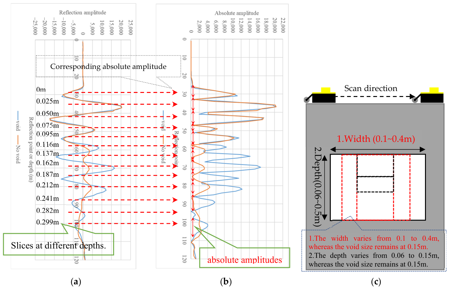
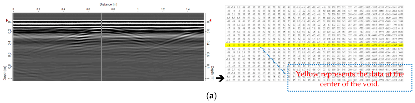
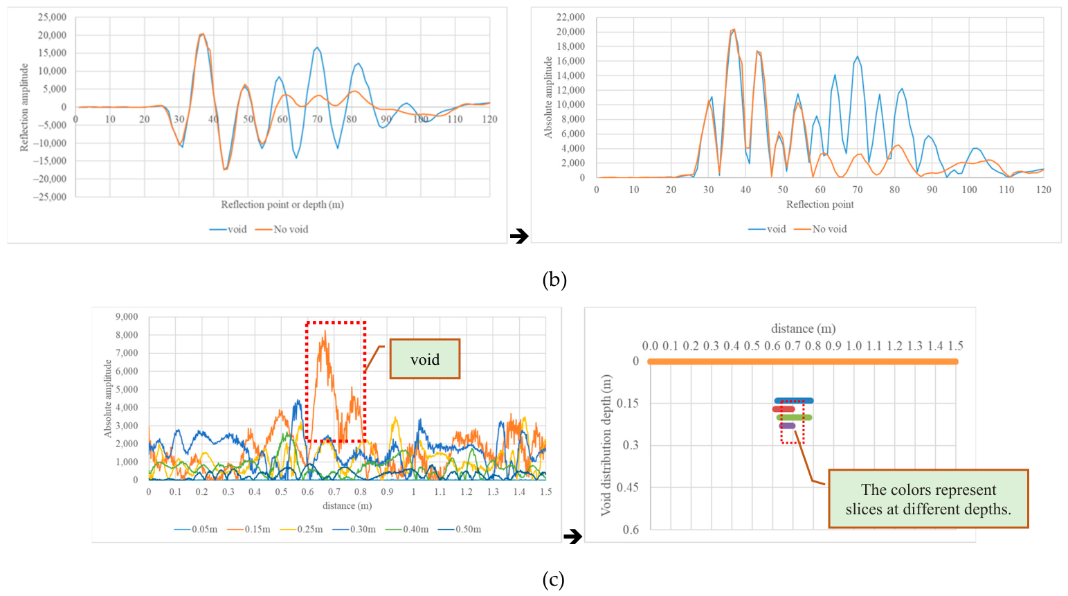
Defect features within the material, expressed as absolute amplitudes, were extracted according to the reflection behavior of electromagnetic waves emitted by GPR as they propagated through the material and were analyzed across different depth slices, as shown in Figure 1a,b. The various depth slices were estimated using the standard wave velocity, as illustrated in Figure 1a, and the absolute amplitudes corresponding to different slice thicknesses were subjected to differentiation processing, including statistical analysis and standard deviation calculations, as shown in Figure 1b. As shown in Figure 1, the boundaries at different depths and widths within the material were analyzed to quantify the defect areas. According to the principles of electromagnetic wave propagation, the dielectric constant of air is 1, ranging from 4 to 10 for concrete and from 3 to 6 for sand. The reflection coefficient represents phase changes (R = ±1) at different interfaces, as well as energy attenuation behavior at the interface of the incident material. When a material contains air defects (dielectric constant = 1) surrounded by material with a dielectric constant of 4, the resulting dielectric contrast manifests as changes in amplitude and wave velocity (see Figure 1 for absolute amplitude differences with and without voids). The behavior at interfaces with varying reflection coefficients is less directly relevant to the method proposed in this study.

2.2. Absolute Amplitude Differentiation

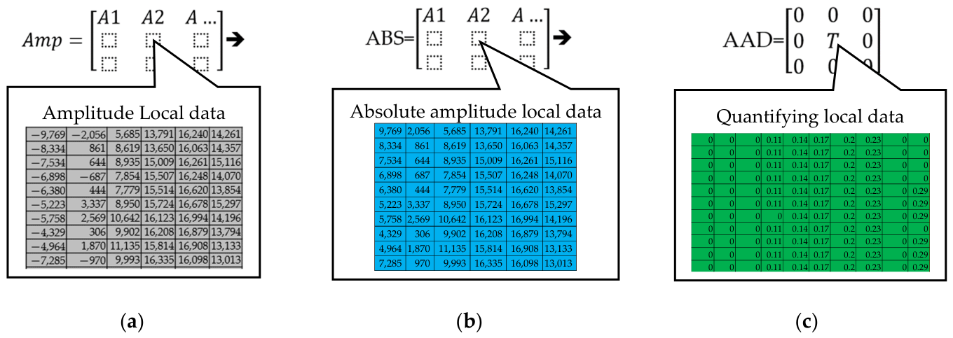
As shown in Figure 1, GPR reflection features (reflection points and absolute amplitudes) were extracted. The absolute amplitude represents reflections caused by voids within the material, while the corresponding reflection points indicate the relative depths of these voids. Following statistical analysis of the original GPR measurement data matrix at a given depth, reflections (absolute amplitudes) from material defects exceeding that depth and from anomalous locations were screened out to delineate the quantitative defect area. The definition of absolute amplitude differentiation is illustrated in Figure 2.

Assuming the distribution of stratum materials remains consistent within the same environment, their reflection behavior and amplitude should be similar across different depths. However, if air voids are present within the material at any depth, the reflection amplitude will change significantly, as shown in Figure 1 (comparing reflections with and without voids). Therefore, by converting the reflection signal of a given length at a specific location into absolute amplitude and calculating the mean and standard deviation, continuous anomalous signals can be identified at any scan location and within any depth slice. This approach provides a scientific basis for determining the presence of voids within the material. For any depth slice within the material matrix, results in the absence of void features should fall within the mean absolute amplitude ± standard deviation at that depth (representing the no-void reflection state). Results outside this range (representing the void-containing reflection state at that depth) are identified using the following absolute amplitude differentiation discriminant formula:

$$\mathrm{No}\text{-}\mathrm{void} \mathrm{state} < \mathrm{AAD} = \left[\begin{array}{ccc}0& 0& 0\\ 0& T& 0\\ 0& 0& 0\end{array}\right] <\mathrm{void}\text{-}\mathrm{containing} \mathrm{state}$$

(1)

For an m × n time-domain matrix, convert the n-axis (amplitude) to absolute values, then use the mean-plus-standard-deviation threshold method to extract anomalous high-amplitude points. This belongs to the principle of statistical outlier detection. This method is based on the normal distribution assumption: most data concentrates around the mean, with values deviating by more than 1σ, suitable for detecting reflection signal anomalies. Converting to absolute values avoids interference from negative amplitudes, making it ideal for identifying defects or strong reflections in time-domain images. The AAD principle formula is as follows:

Let matrix $\mathrm{M}\in R^{m\times n}$, where the m-axis (i = 1…m) represents measurement distance, and the n-axis (j = 1…n) represents amplitude $A_{i,j}$.

Step 1: Absolute Value Conversion

$$\left|A_{i,j}\right|=abs\left(A_{i,j}\right)$$

(2)

Step 2: Statistical Parameters

$$\mathrm{Mean}: \mathsf{\mu }={\displaystyle \frac{1}{mn}}{\sum }_{i=1}^m{\sum }_{j=1}^n\left|A_{i,j}\right|$$

(3)

$$\mathrm{Standard} \mathrm{Deviation}: \mathsf{\sigma }=\sqrt{{\displaystyle \frac{1}{mn}}{\sum }_{i=1}^m{\sum }_{j=1}^n{\left(\left|A_{i,j}\right|-\mu \right)}^2}$$

(4)

$$\mathrm{Threshold}: \mathrm{T}=\mathsf{\mu }+\mathsf{\sigma }$$

(5)

Step 3: Anomaly Extraction

$$\mathsf{\Omega }=\left\{\left(i,j\right)|\left|A_{i,j}\right|>T\right\}$$

(6)

The parameters corresponding to the above formulas are explained below:

• M: Time-domain matrix (m × n);
• A_i,j: Amplitude at position (i,j);
• μ: Mean of absolute amplitudes;
• σ: Standard deviation of absolute amplitudes;
• T = μ + σ: Anomaly threshold (1σ method);
• Ω: Set of anomalous positions.

3. Research Details

3.1. Experiment

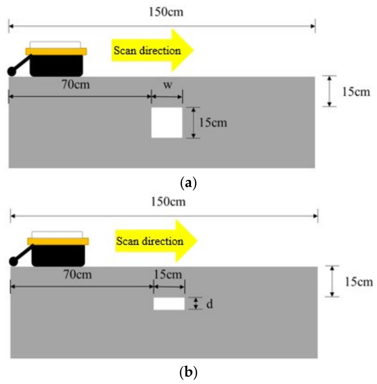
This study utilized MALÅ GPR antennas with center frequencies of 2.3 GHz, 1.2 GHz, 1 GHz, 800 MHz, and 750 MHz, as shown in Figure 3. Pavement thicknesses on general roads and river/coastal levees typically range from 0.1 to 0.2 m. The primary concern is the progressive deterioration of subsurface voids beneath the pavement. Although signal filtering aids in locating and identifying voids within materials from GPR images, research on quantifying void depth remains limited. The investigation focused on concrete specimens with a thickness of 0.15 m. Two experimental conditions were designed: (1) concrete specimens with widths of 0.10, 0.20, 0.30, or 0.40 m, all containing voids of 0.15 m in size (4 widths × 5 antenna frequencies = 20 experimental datasets), and (2) voids of sizes 0.06, 0.10, or 0.15 m within specimens of 0.15 m width (3 void sizes × 5 antenna frequencies = 15 experimental datasets), as shown in Figure 1c and Figure 4. GPR reflections from these specimens were compared across different antenna frequencies. The experimental combinations were analyzed using absolute amplitude differentiation (AAD), as illustrated in Figure 4.

3.2. Reflection Signal Extraction and Analyses

The original GPR profile images were converted into matrix data (absolute amplitudes), as shown in Figure 5a,b. Differentiation-based screening was then applied across the entire array to retain anomalous feature data. For example, as illustrated in Figure 1 and Figure 2 and Equations (1)–(5), the original matrix produces no abnormal features at any depth or position in the absence of voids. However, voids at any depth or position generate abnormal features exceeding the mean plus one standard deviation. This enabled the quantitative extraction of void depths and spatial extents, with XY distribution plots generated for comparison, as shown in the right panel of Figure 5c. Based on the spectrum extracted from the reflection (amplitude variation) matrix, absolute amplitude analyses were conducted across six depth slices corresponding to 0–0.50 m depths. The screened feature points from each depth layer were then plotted as XY scatter diagrams of survey distance versus vertical depth (Figure 5c). The left panel of Figure 5c shows that the 0.15 m slice depth corresponds to the interface between the void and the concrete, where the reflection intensity reaches its maximum. The absolute amplitude slices at different depths indicate that the amplitude at 0.05 m is significantly lower than those at other depths, while amplitudes beyond 0.3 m decrease due to wave attenuation. At the void location (0.05 m × 0.15 m), distinct amplitude variations are observed. These variations were subsequently subjected to statistical screening, with the results presented in the right panel of Figure 5c.

4. Research Results

4.1. Results for Voids of a Fixed Size but Varying Widths (0.1–0.4 m)

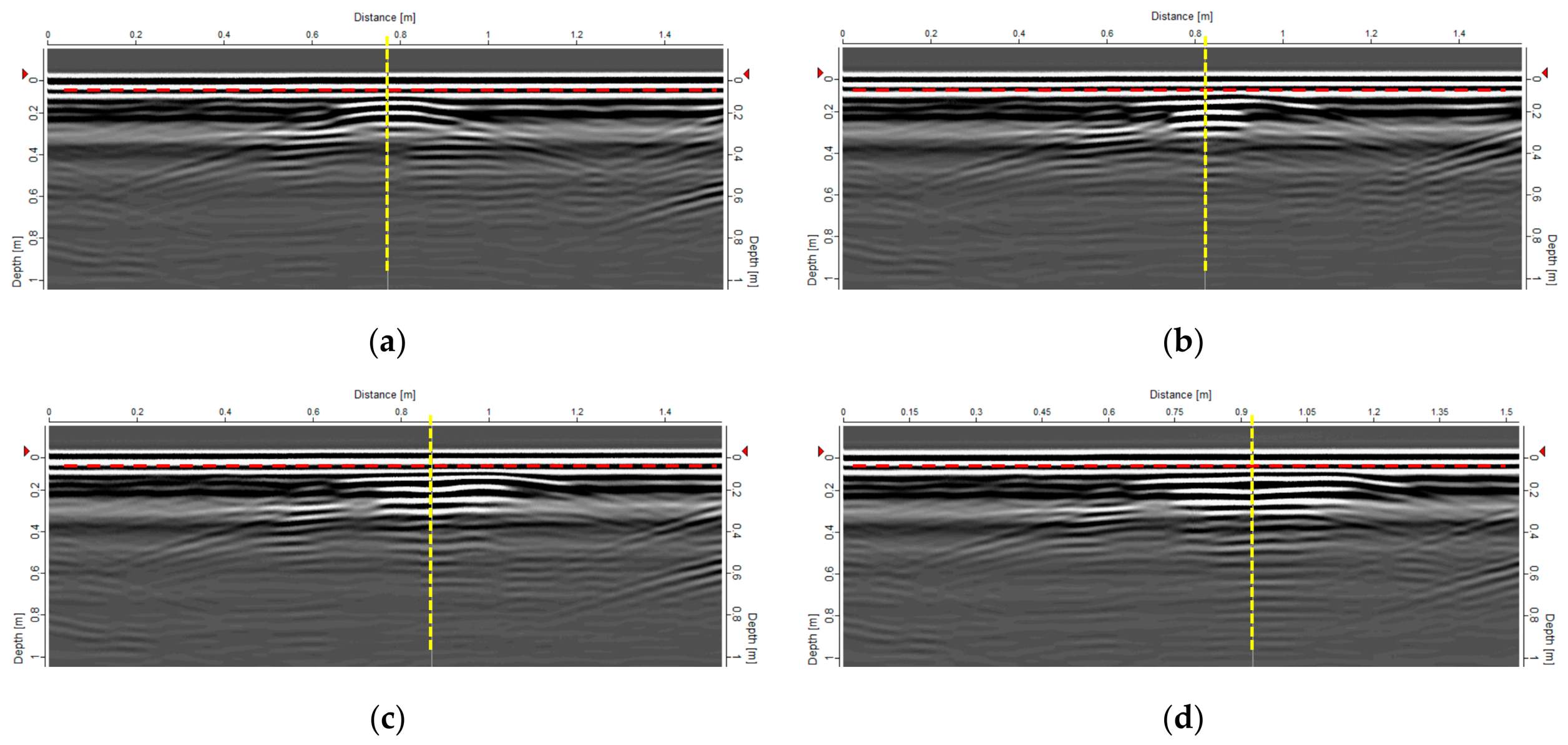
Five MALÅ GPR antennas with center frequencies of 2.3 GHz, 1.2 GHz, 1 GHz, 800 MHz, and 750 MHz, were used to scan 0.15 m thick concrete specimens containing 0.15 m voids with widths ranging from 0.10 to 0.40 m, generating a total of 35 experimental datasets (5 frequencies × 7 specimens). Since the AAD processing workflow is identical across cases, data from a 1 GHz ground-penetrating radar (GPR) antenna are used here for demonstration purposes. The corresponding GPR profile images, horizontal-axis slices, and depth-axis slices are presented in Figure 6, Figure 7 and Figure 8.

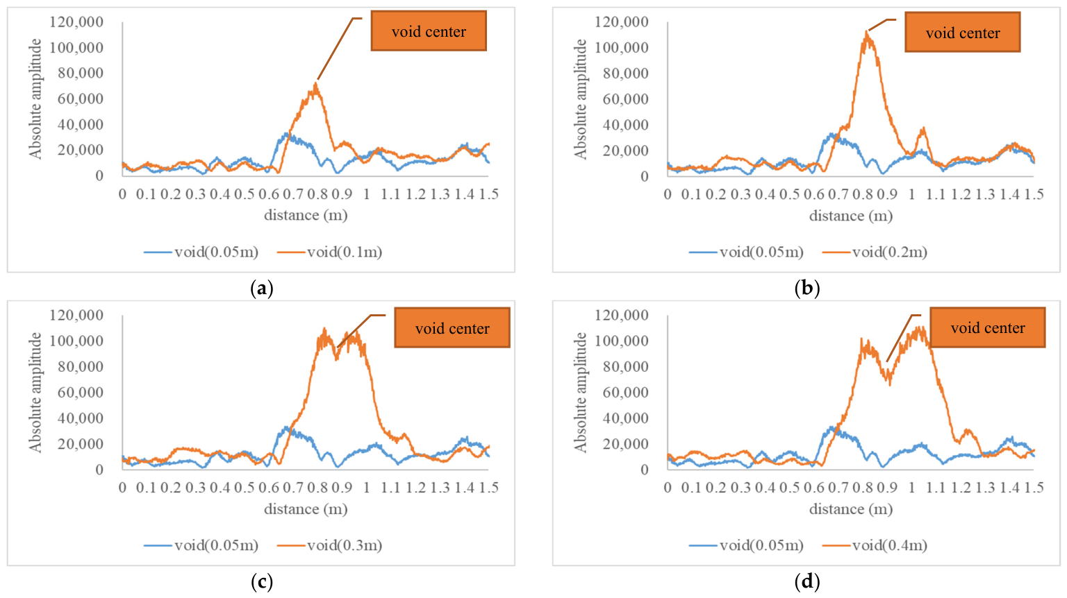
The results of absolute amplitude differentiation (AAD) analyses are shown in Figure 6, presenting absolute amplitude variations at a 0.15 m depth slice with survey distance along the horizontal axis (red dashed line). As illustrated in Figure 7, with a fixed void size of 0.15 m, the absolute reflection amplitude intensity increases gradually with void width and stabilizes when the width exceeds 0.20 m.

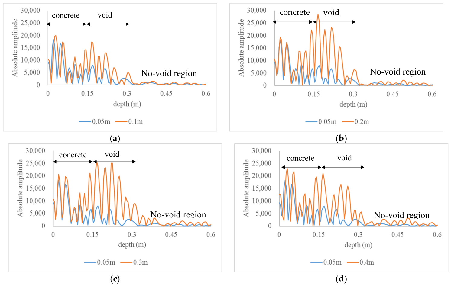
The analyses also show how absolute amplitude varies over the 0–0.6 m depth range; in Figure 6, the depth direction is taken as the vertical axis (yellow dashed line). As illustrated in Figure 8, with void depth fixed at 0.15 m, the central absolute reflection amplitude intensity peaks over void widths of 0.15–0.30 m and stabilizes beyond 0.3 m width. Beyond a depth of 0.3 m, where no voids are present, the absolute reflection amplitude transitions to no-void behavior. This indicates that voids in concrete produce absolute/reflected amplitudes at their upper and lower boundaries greater than those in surrounding no-void material (Figure 8).

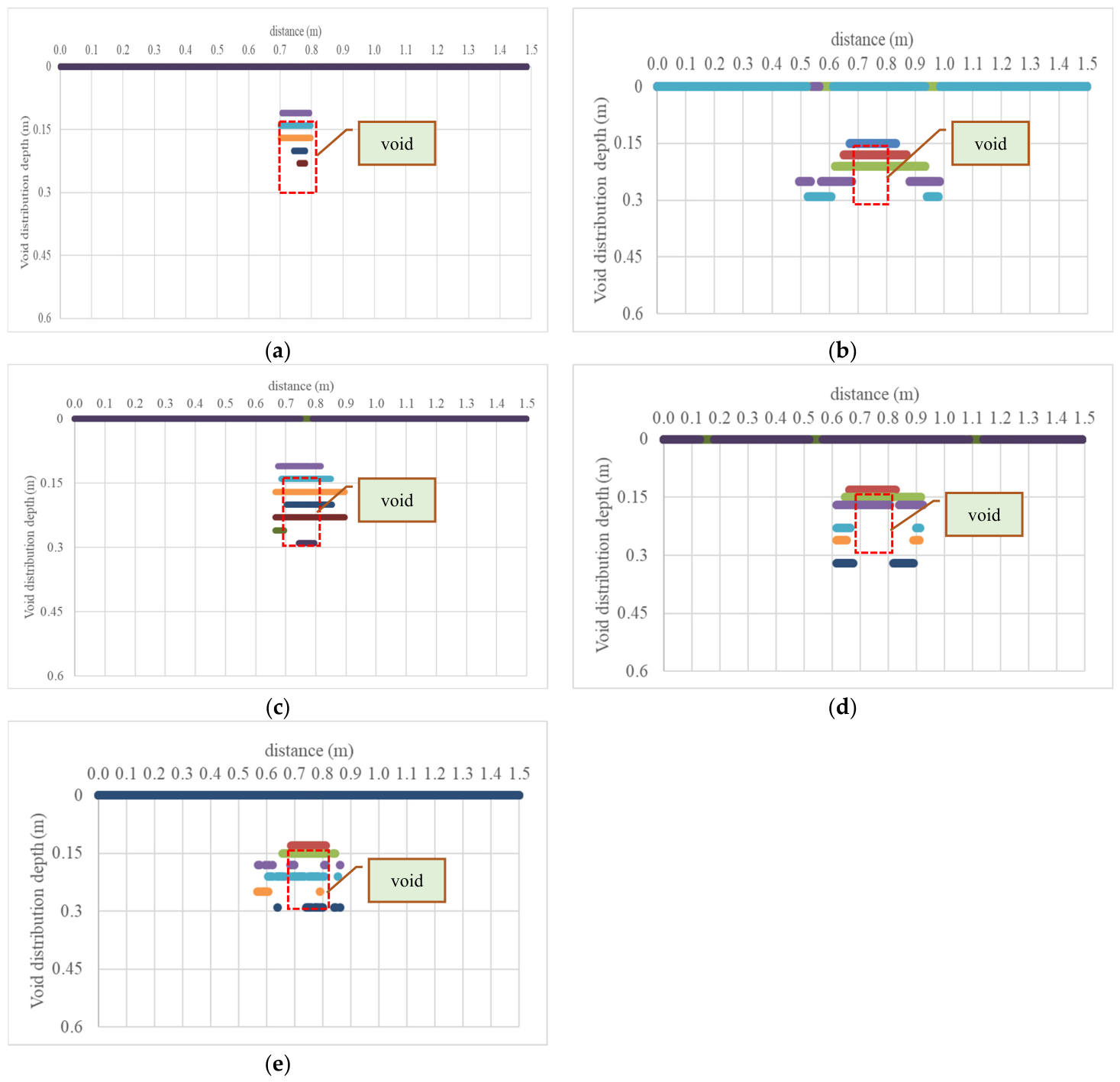
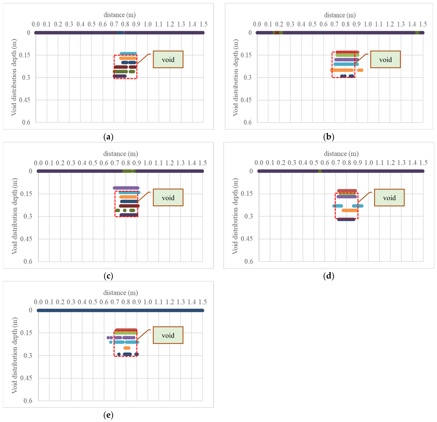
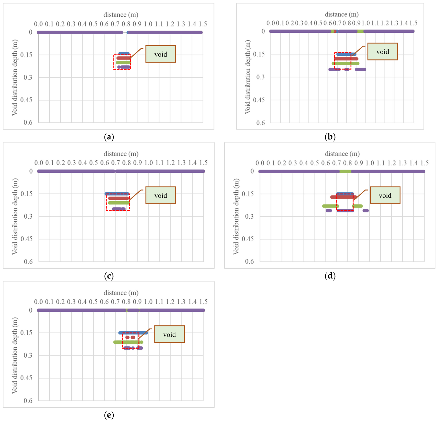
Figure 9, Figure 10, Figure 11 and Figure 12 display the postscreening results of the absolute amplitude differentiation analyses, which are presented as XY scatter plots of survey distance versus vertical depth, with the red boxes indicating the actual void location. When the void width is 0.1 m, all five antenna sets can capture distinct reflection features; however, the reflection amplitudes for depths greater than 0.2 m are relatively weak. As shown in Figure 9a–e, the 750 MHz and 1 GHz antennas obtain more-concentrated void reflections, the 800 MHz and 1.2 GHz antennas collect void reflections with larger edge diffraction, and the 2.3 GHz antenna obtains more-dispersed void reflections. Although the above descriptions of reflection characteristics and phenomena for different antennas under varying void conditions are qualitative, they demonstrate that antennas can distinguish voids of different widths. The results reveal reflection and diffraction behavior under the specified void and boundary conditions.

As illustrated in Figure 10, for a 0.20 m void width, distinct reflection features are captured down to a depth of 0.30 m. Void reflections are concentrated for the 750 MHz, 800 MHz, and 1.0 GHz antennas, whereas bottom reflections from the void are relatively weak for the 1.2 GHz and 2.3 GHz antennas (Figure 10a–e).

Figure 11 shows that when the void width is 0.3 m, distinct reflection features can be identified down to a depth of 0.3 m. Moreover, the reflections from the void are relatively concentrated across antenna frequencies ranging from 750 MHz to 2.3 GHz, as illustrated in Figure 11a–e.

For a 0.40 m void width, distinct reflection features are extracted down to a depth of 0.30 m (Figure 12). Void reflections are concentrated across all antenna frequencies except 750 MHz, for which the captured width-related features are relatively conservative.

The results presented in Figure 9, Figure 10, Figure 11 and Figure 12 indicate that all antennas exhibit good sensitivity for void detection. For voids within concrete, the absolute amplitude differentiation analysis reveals continuous reflection behavior along the depth axis. The lateral boundaries along the survey distance can be used to determine the width of the voids, whereas the superposition of continuous reflections along the depth axis effectively indicates the void thickness. The proposed method is straightforward and efficient; absolute amplitude differentiation can be applied at any selected depth, providing a rapid approach for assessing potential voids within the material.

Table 1. Experimental Analysis Results for Voids with Fixed Depth and Widths of 0.1–0.4 m.

Antenna (MHz)	750 MHz	Accuracy (%)	800 MHz	Accuracy (%)	1 GHz	Accuracy %	1.2 GHz	Accuracy %	2.3 GHz	Accuracy %
Void Width (m)	T1/T0 (m2)		T1/T0 (m2)		T1/T0 (m2)		T1/T0 (m2)		T1/T0 (m2)
0.1	0.009/0.015	61	0.017/0.015	116	0.018/0.015	119	0.016/0.015	106	0.010/0.015	64
0.2	0.019/0.030	63	0.032/0.030	106	0.025/0.030	82	0.021/0.030	70	0.015/0.030	50
0.3	0.022/0.045	49	0.041/0.045	92	0.038/0.045	84	0.028/0.045	63	0.022/0.045	48
0.4	0.035/0.060	60	0.054/0.060	90	0.049/0.060	82	0.38/0.060	63	0.28/0.060	47
Average %		58.3	Average %	101.0	Average %	91.8	Average %	75.5	Average %	52.3

compares the total T₀ data points of the designed void with the total T₁ data points associated with reflection anomalies. The results indicate that all five antennas exhibit favorable reflection behavior at the void interface. However, certain antennas show energy attenuation and scattering at the void boundaries and base, which introduce errors in the total T₁/T₀ data. In addition, the antennas respond differently to variations in void location and depth. The total T₁ data points for void reflections are most accurately captured at 800 MHz and 1 GHz. In contrast, the other antennas fail to fully capture the T₁ signal characteristics at the void interface and bottom due to energy attenuation and scattering. The results of the AAD analysis for a void with a fixed depth of 0.15 m (width range: 0.1–0.4 m) are summarized in Table 1.

4.2. Results for Voids of a Fixed Width but Varying Sizes (0.06–0.15 m)

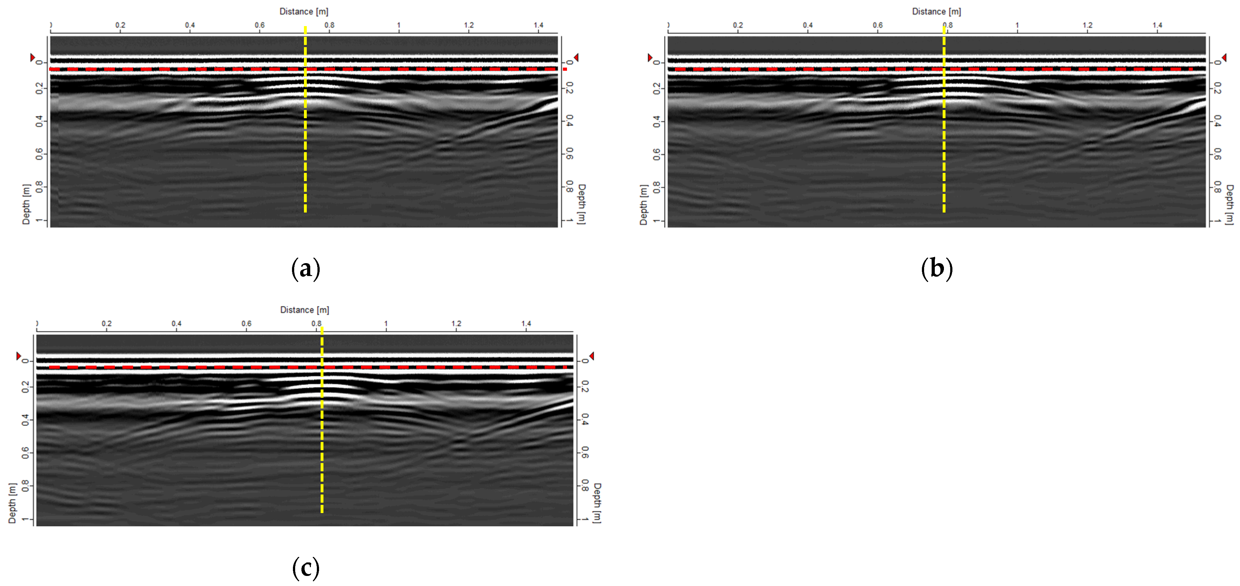
Five MALA GPR antennas with frequencies of 2.3 GHz, 1.2 GHz, 1 GHz, 800 MHz, and 750 MHz were used to scan 0.15 m thick concrete specimens containing voids with a fixed width of 0.15 m and heights ranging from 0.06 to 0.15 m, resulting in a total of 15 experimental datasets. As described in Section 4.1, the data obtained from the 1 GHz ground-penetrating radar (GPR) antenna are used for demonstration. The corresponding GPR profiles, along with the horizontal and depth slices, are presented in Figure 13, Figure 14 and Figure 15.

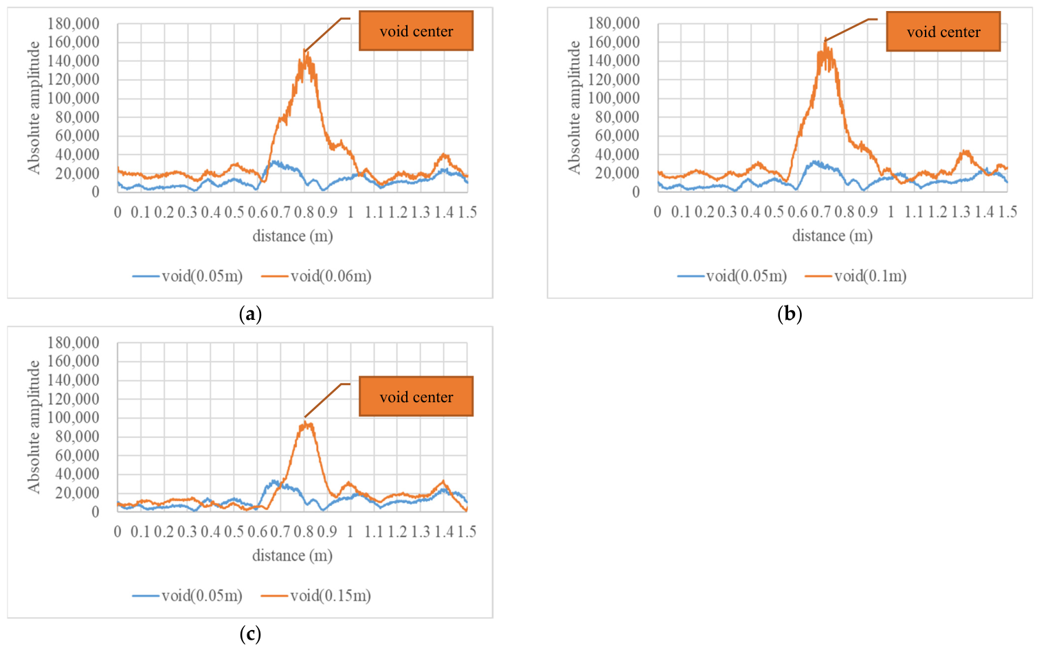
The results of the absolute amplitude differentiation (AAD) analysis are presented in Figure 13, showing the absolute amplitude variation at a slice depth of 0.15 m, with the survey distance represented along the horizontal axis (red dashed line). As shown in Figure 14, for void sizes of 0.06 m, 0.10 m, and 0.15 m under a fixed width of 0.15 m, the differences in absolute reflection amplitude are not significant. However, a decrease is observed for the 0.15 × 0.15 m void, indicating that larger void sizes lead to more pronounced energy attenuation. Furthermore, as illustrated in Figure 7 and Figure 14, when the void width and size within the material reach a certain scale, a peak value is observed. The ratio of the absolute reflection amplitude of void-containing material to that of non-void material ranges from approximately 10 to 16, indicating that the presence of voids produces strong and distinguishable reflection signals. This characteristic enables effective extraction of void features and supports objective quantitative analysis through statistical screening.

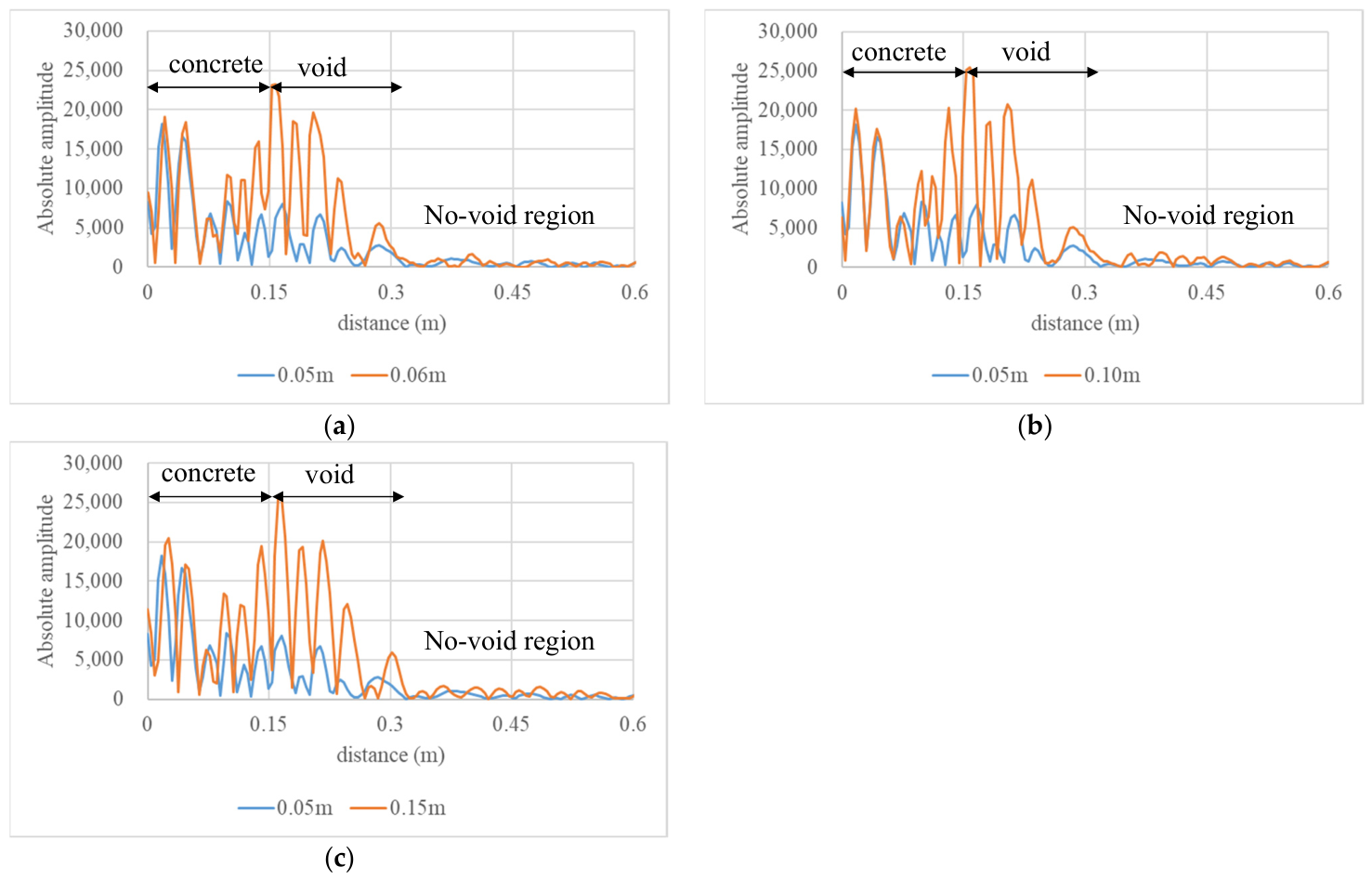
As shown in Figure 15, when the void depth is fixed at 0.15 m, the central absolute reflection amplitude is highest for void sizes ranging from 0.06 to 0.15 m. Meanwhile, beyond 0.30 m along the depth axis, the material transitions into a no-void region, and the absolute reflection amplitude correspondingly exhibits no-void reflection behavior. This indicates that, when voids are present within concrete, the absolute reflection amplitudes at both the upper and lower boundaries of the void are greater than those of the surrounding intact material, as illustrated in Figure 15.

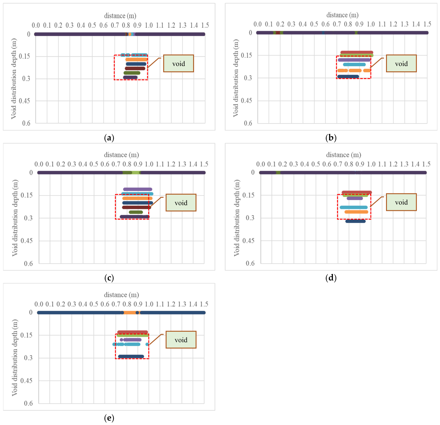
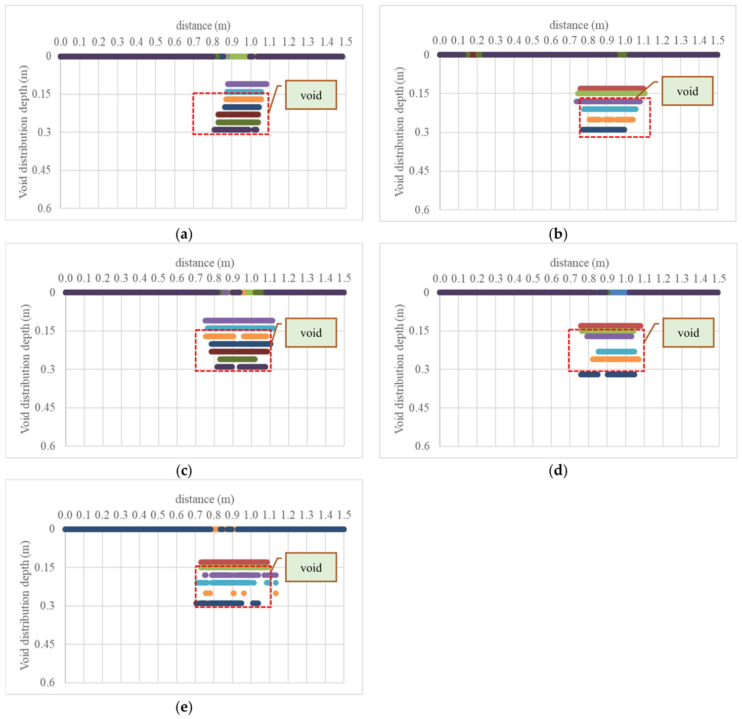
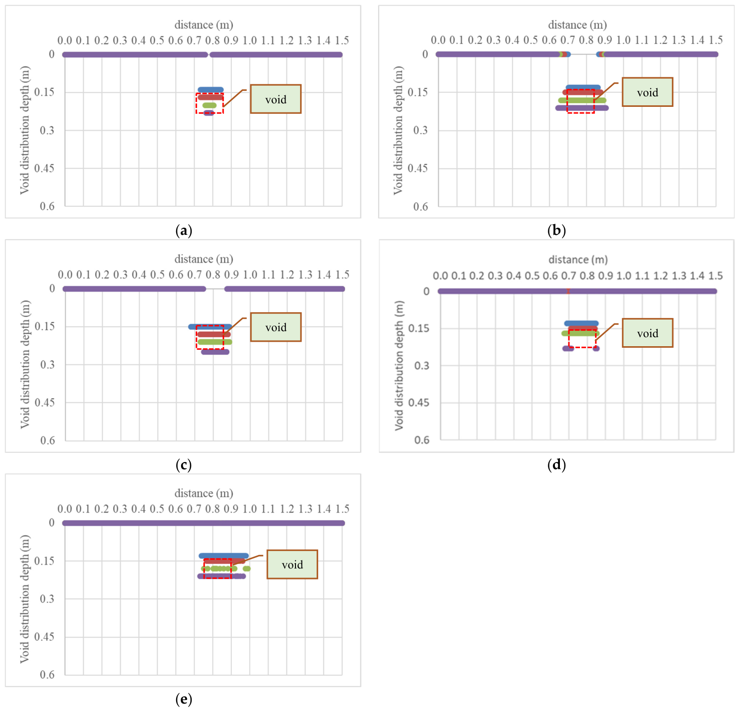
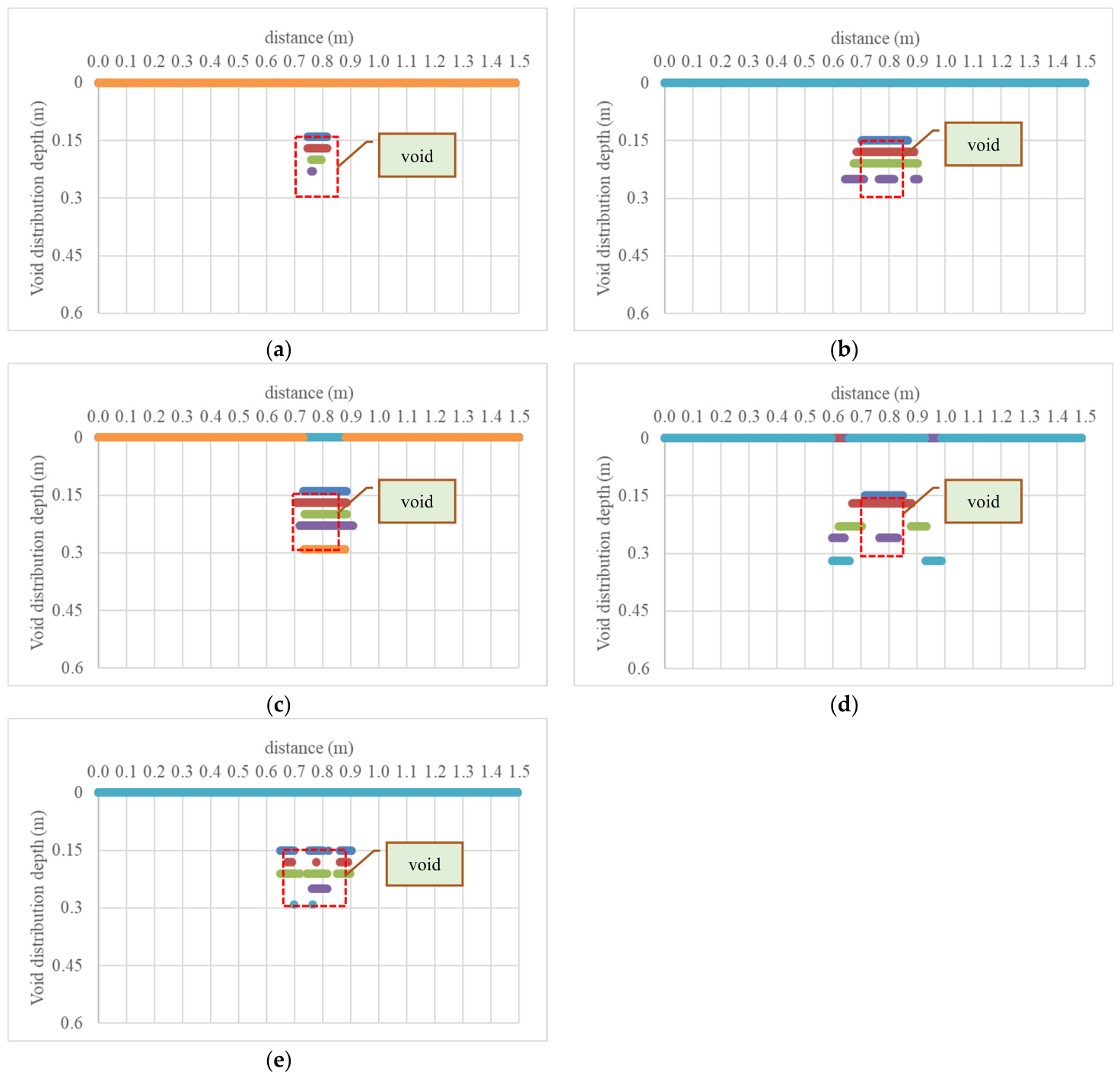
When the void width is fixed at 0.15 m, five GPR antennas (2.3 GHz, 1.2 GHz, 1 GHz, 800 MHz, and 750 MHz) are used to investigate void sizes of 0.06 m, 0.10 m, and 0.15 m. After applying the absolute amplitude differentiation (AAD) analysis, the results are presented as XY scatter plots of survey distance versus depth, with red boxes indicating the actual void locations, as shown in Figure 16, Figure 17 and Figure 18. As shown in Figure 16, for a void width of 0.15 m and a void size of 0.06 m, all five antennas are able to extract distinct reflection features down to a depth of 0.21 m. Among them, the AAD results for the 750 MHz antenna are largely confined within the void boundaries, whereas those for the other antennas extend beyond the void limits, indicating stronger edge diffraction effects at the void boundaries, as illustrated in Figure 16a–e.

As shown in Figure 17, when the void size is 0.10 m, distinct reflection features can be extracted down to a depth of 0.25 m. The extraction and screening results are consistent with those presented in Figure 16, as illustrated in Figure 17a–e.

As shown in Figure 18, when the void size is 0.15 m, distinct reflection features can be extracted down to a depth of 0.30 m. The extraction and screening results are consistent with those presented in Figure 17, as illustrated in Figure 18a–e.

A comparison of Table 1 and

Table 2. Experimental analysis results for voids with fixed width and depths of 0.06–0.15 m.

Antenna (MHz)	750 MHz	Accuracy (%)	800 MHz	Accuracy (%)	1 GHz	Accuracy %	1.2 GHz	Accuracy %	2.3 GHz	Accuracy %
Void Depth (m)	T1/T0 (m2)		T1/T0 (m2)		T1/T0 (m2)		T1/T0 (m2)		T1/T0 (m2)
0.06	0.006/0.009	69	0.010/0.009	111	0.010/0.009	111	0.008/0.009	87	0.007/0.009	81
0.1	0.009/0.015	63	0.016/0.015	108	0.015/0.015	97	0.014/0.015	96	0.012/0.015	81
0.15	0.010/0.023	45	0.026/0.023	117	0.025/0.023	110	0.024/0.023	107	0.015/0.023	65
Average %		59.0	Average %	112.0	Average %	106.0	Average %	96.7	Average %	75.7

shows that all five antenna groups exhibit good reflection characteristics at the void interface. However, energy attenuation and scattering occur at the boundaries and bottom of the void for the 750 MHz and 2.3 GHz antennas, leading to errors in the total T₁/T₀ data. In addition, the antenna responses vary with different combinations of void location and width. The total T₁ data points for void reflections are most accurately captured within the 800 MHz, 1 GHz and 1.2 GHz frequency range. The results of the AAD analysis for a void with a fixed width of 0.15 m (depth range: 0.06–0.15 m) are presented in Table 2.

4.3. Case Analyses

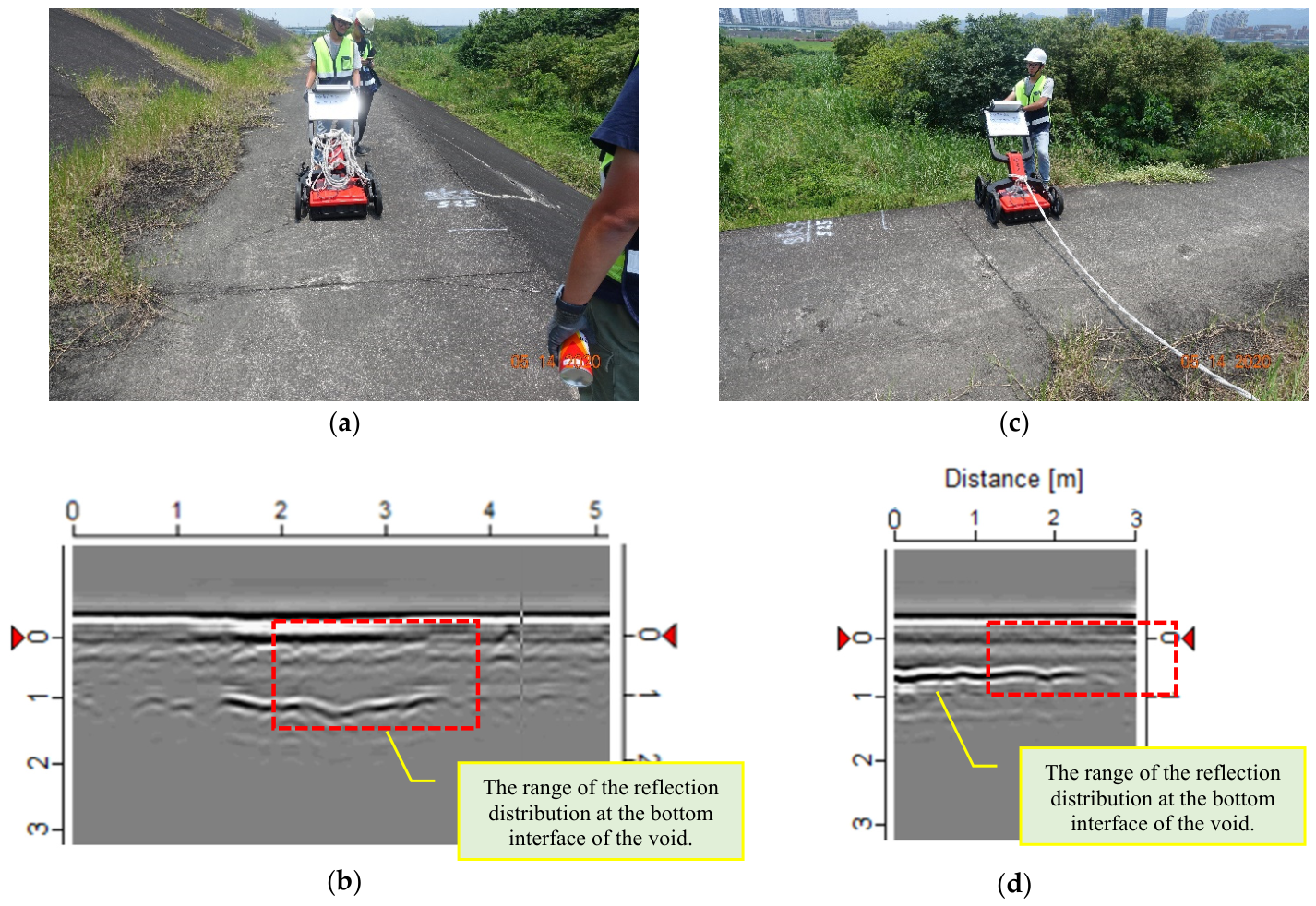
This study investigated internal scour in front of a levee berm along the longitudinal direction, with additional transverse survey lines, as illustrated in Figure 19. A preliminary assessment of the scour length, width, and depth was conducted based on the GPR profile images, and the results are as follows:

• The transverse survey line indicated that the anomalous scour length was 2 m, with depths of 0.91 m on the left side and 0.75 m on the right side.
• The longitudinal survey line in front of the berm showed that the anomalous scour width was 2 m and the depth was 1 m.
• Based on these results, the total scour area at this location was approximately 4 m². Given a GPR profile depth of approximately 0.75–1.00 m, the scour volume was estimated to be approximately 3.32 m³.

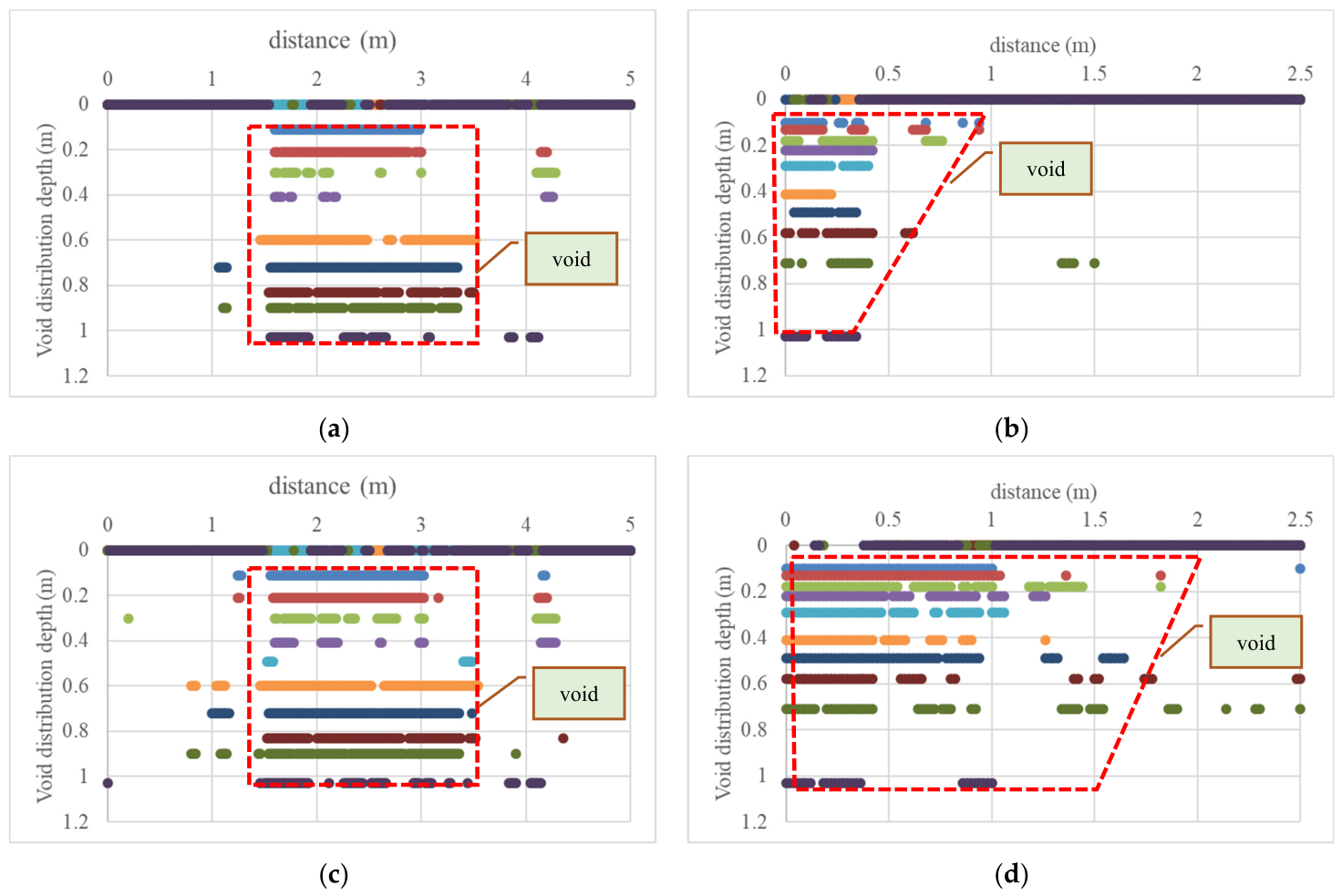
Absolute amplitude differentiation analyses were performed for the longitudinal and transverse survey lines of the levee berm, as shown in Figure 20. After statistical screening at various slice depths, the scour length, width, and depth were evaluated, and the results are as follows:

• Based on the transverse measurement line, the abnormal length along the top edge was determined to be 2 m, the abnormal length along the bottom edge was 1.5 m, and the depth was 1 m.
• Based on the longitudinal survey line in front of the berm, the anomalous width was determined to be 2 m, with a depth of 1 m.
• The void distribution obtained after AAD processing of the original data was approximately 2 m³. By enhancing the reflection intensity through filtering, AAD processing yielded more detailed anomalous void distribution data, consistent with the profile and excavation results.
• According to these results, the scour area at this location was approximately 4 m². Given a GPR profile depth of approximately 1 m, the scour volume was estimated to be approximately 3–4 m³ (average: approximately 3.5 m³), as shown in Figure 20.

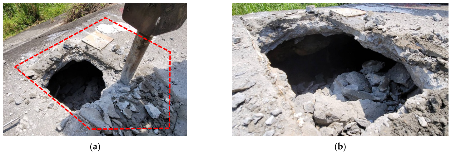
As shown in Figure 21, on-site excavation revealed the extent of the scour as follows:

• The transverse survey line indicated an anomalous length of 2 m, with depths of 0.91 m on the left side and 0.75 m on the right side.
• The longitudinal survey line in front of the berm indicated an anomalous width of 2 m and a depth of 0.96 m.
• Based on these results, the scour area at this location was approximately 4 m². Given a GPR profile depth of approximately 0.75–0.96 m, the scour volume was estimated to be approximately 3–4 m³ (average: approximately 3.58 m³).

A comparison of the scour volume results shown in Figure 19, Figure 20 and Figure 21 indicates that the profile-based estimation was close to the post-excavation result, whereas the value obtained from the absolute amplitude differentiation analysis was smaller. This discrepancy arises because the present method analyzes the initial signals; when the void within the material is larger and wider, the reflection intensity is considerably lower, which is consistent with the findings discussed in Section 4.1 and Section 4.2. Therefore, to better reflect actual conditions, signal enhancement followed by absolute amplitude differentiation analysis can improve the accuracy of scour volume estimation, as shown in Figure 20. The proposed method is thus a feasible approach for quantifying voids within materials.

Table 3. The results of the excavation comparison for each case.

Scanning Direction	Longitudinal		Transverse		Volume (m3)
Identification Method	Length (m)	Depth (m)	Length (m)	Depth (m)
Actual excavation	2	0.96	2	0.75~0.91	≈3.58
Filtered image	2	1	2	0.75~0.91	≈3.32
AAD method	2	1	2	1	≈3.50

shows the results of the subjective interpretation of the GPR profiles, the objective interpretation based on AAD analysis, and the actual excavation volume.

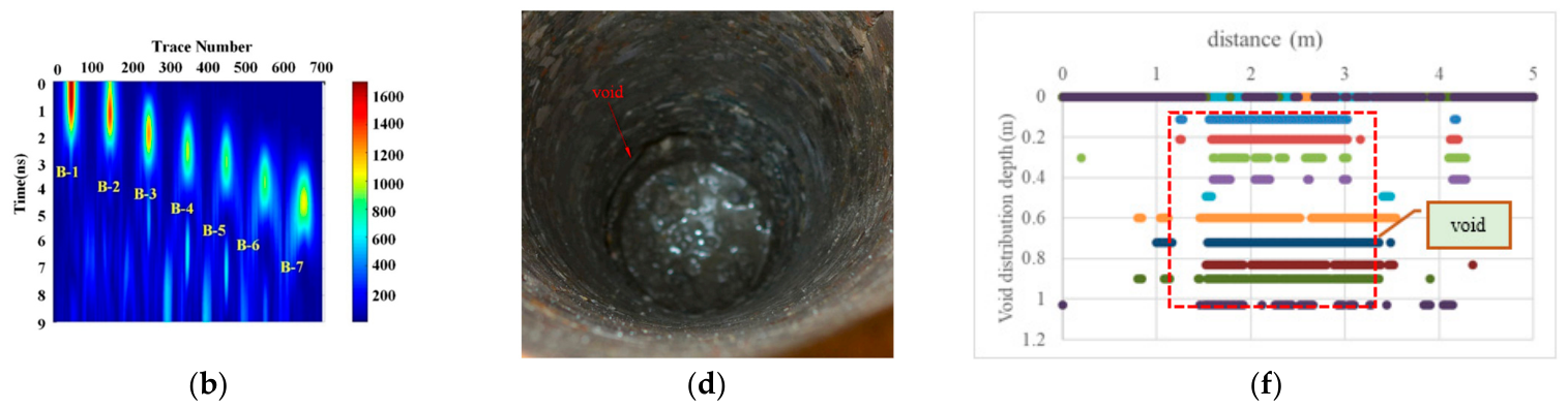
Reference investigated the design of a void measuring 0.1 × 0.1 m with a depth of less than 0.55 m. A cross-sectional image of the material containing the void was scanned at 1 GHz using a mine radar system. Conversion of the CWT and time-domain data to the time-frequency domain revealed energy concentration in the void region [12]. According to Ref [13], an optimized five-step feature-enhancement post-processing protocol was established, and the FDTD results showed that voids are associated with GPR patterns such as irregular banded stripes, hyperbolas, cross shapes, bowl shapes, or plain reverberation. In the literature, a bright white-black band is the most common feature associated with voids. A suspicious region exhibiting this feature was randomly selected from a survey line, and the presence of a void was confirmed by coring [13]. In this study, the void identification results reported in the literature are compared with the AAD results. Reference showed that voids at different burial depths can be identified, while Reference used filtering to enhance the image intensity of anomalous regions for void localization. In this study, we assume that the reflection intensity of the material is similar at any depth. After statistical screening using AAD on the total amplitude data at each depth, a void distribution map is extracted, with the X-axis representing the length range and the Y-axis representing the depth range, as shown in Figure 22.

5. Conclusions

• This study proposes an absolute amplitude differentiation (AAD) method, and the quantitative results obtained for voids of various widths and sizes within concrete specimens are highly informative. Reflection signals were collected from five antenna sets, capturing reflection amplitudes associated with internal material defects. Differential screening of the material matrix, based on statistical analyses of multiple slices, enabled the objective determination of void widths and sizes for area evaluation.
• Through simple absolute-value operations combined with statistical analyses, the material matrix data obtained from ground-penetrating radar (GPR) were subjected to statistical screening and differentiation. Void characteristics, represented by absolute amplitudes, were extracted and reorganized along horizontal and vertical axes. This approach enabled accurate determination of void locations and sizes, as illustrated in Figure 9, Figure 10, Figure 11, Figure 12, Figure 16, Figure 17 and Figure 18.
• This study applied AAD analysis in indoor environments, where statistical screening of slices at various depths allowed accurate estimation of void sizes. However, results from outdoor experiments indicate that, in complex environments, insufficient electromagnetic wave energy and rapid attenuation in air can reduce the accuracy of AAD assessments. Therefore, enhanced signal filtering is recommended to improve penetration capability. In situations lacking experienced personnel, rapid and objective methods for detecting voids in shallow materials remain valuable, particularly for evaluating infrastructure such as roads and river or coastal dikes.

References

1. Water Resources Agency, Ministry of Economic Affairs. Number of Existing River Flood Control Facilities in 113th Year; Official Statistical Report of the Water Resources Agency: Taipei, Taiwan, 2025.
2. Water Resources Agency, Ministry of Economic Affairs. The Existing Coastal Protection (Sea-Dike) Works in 113th Year; Official Statistical Report of the Water Resources Agency: Taipei, Taiwan, 2025.
3. Water Resources Agency, Ministry of Economic Affairs. Damage Conditions of River Flood Control and Drainage Facilities from Years 106 to 112; Statistical Bulletin of the Water Resources, Ministry of Economic Affairs: Taipei, Taiwan, 2024.
4. Water Resources Agency, Ministry of Economic Affairs. Damage Conditions of River Flood Control Facilities Caused by Natural Disasters in Year 113; Official Statistical Report of the Water Resources Agency: Taipei, Taiwan, 2025.
5. Shi, B.Y. Ground Penetrating Radar Road Inspection Project Management—The Case of Taoyuan City. Master’s Thesis, National Central University, Taoyuan, Taiwan, 2025. [Google Scholar]
6. Wang, Y.W. Deep Learning-Driven Automated Detection of Voids and Defects in Levee Ground Penetrating Radar Imagery. Master’s Thesis, Chaoyang University of Technology, Taichung, Taiwan, 2025. [Google Scholar]
7. Wang, B.Y. The Application of Ground Penetration Radar on the Detection of Ground Disturbances and Underground Buried Objects. Master’s Thesis, National Cheng Kung University, Tainan, Taiwan, 2024. [Google Scholar]
8. Lin, Y.C. Effectiveness of 3D GPR Compared with 2D GPR for Defect Detection. Master’s Thesis, National Yang Ming Chiao Tung University, Hsinchu, Taiwan, 2023. [Google Scholar]
9. Chuang, K.D. A Preliminary Study on Methods for Detecting Road Voids Using Ground-Penetrating Radar; Institute of Transportation, Ministry of Transportation and Communications: Taipei, Taiwan, 2022.
10. Xiong, X.T.; Meng, A.X.; Lu, J.; Tan, Y.Q.; Chen, B.; Tang, J.M.; Zhang, C.; Xiao, S.Q.; Hu, J.Y. Automatic detection and location of pavement internal distresses from ground penetrating radar images based on deep learning. Constr. Build. Mater. 2024, 411, 134483. [Google Scholar] [CrossRef]
11. Hu, H.B.; Fang, H.Y.; Wang, N.N.; Ma, D.; Dong, J.X.; Li, B.; Di, D.Y.; Zheng, H.B.; Wu, J. Defects identification and location of underground space for ground penetrating radar based on deep learning. Tunn. Undergr. Space Technol. 2023, 140, 105278. [Google Scholar] [CrossRef]
12. Yu, Q.Q.; Li, Y.X.; Luo, T.Y.; Zhang, J.; Tao, L.; Zhu, X.; Zhang, Y.; Luo, L.F.; Xu, X.X. Cement pavement void detection algorithm based on GPR signal and continuous wavelet transform method. Sci. Rep. 2023, 13, 19710. [Google Scholar] [CrossRef]
13. Zhang, J.; Lu, Y.M.; Yang, Z.; Zhu, X.; Zheng, T.; Liu, X.; Ting, Y.G.; Li, W.G. Recognition of void defects in airport runways using ground-penetrating radar and shallow CNN. Autom. Constr. 2022, 138, 104260. [Google Scholar] [CrossRef]
14. Wu, X.L.; Bao, X.H.; Shen, J.; Chen, X.S.; Cui, H.G. Evaluation of void defects behind tunnel lining through GPR forward simulation. Sensors 2022, 22, 9702. [Google Scholar] [CrossRef]
15. Li, N.S.; Wu, R.B.; Li, H.F.; Wang, H.C.; Gui, Z.C.; Song, D.Z. MV-GPRNet: Multi-view subsurface defect detection network for airport runway inspection based on GPR. Remote Sens. 2022, 14, 4472. [Google Scholar] [CrossRef]
16. Li, Y.S.; Liu, C.L.; Yue, G.H.; Gao, Q.; Du, Y.C. Deep learning-based pavement subsurface distress detection via ground penetrating radar data. Autom. Constr. 2022, 14, 104516. [Google Scholar] [CrossRef]
17. Hu, H.B.; Fang, H.Y.; Wang, N.N.; Liu, H.; Lei, J.W.; Ma, D.; Dong, J.S. A study of automatic recognition and localization of pipeline for ground penetrating radar based on deep learning. IEEE Geosci. Remote Sens. Lett. 2022, 19, 4026405. [Google Scholar] [CrossRef]
18. Liu, B.; Ren, Y.X.; Liu, H.C.; Xu, H.; Wang, Z.F.; Cohn, A.G.; Jiang, P. GPRInvNet: Deep learning-based ground penetrating radar data inversion for tunnel linings. IEEE Trans. Geosci. Remote Sens. 2021, 59, 8305–8325. [Google Scholar] [CrossRef]
19. Lei, W.T.; Luo, J.B.; Hou, F.F.; Xu, L.; Wang, R.Q.; Jiang, X.Y. Underground cylindrical objects detection and diameter identification in GPR B-scans via the CNN LSTM framework. Electronics 2020, 9, 1804. [Google Scholar] [CrossRef]
20. Luo, X.H.; Lai, W.L. GPR pattern recognition of shallow subsurface air voids. Tunn. Undergr. Space Technol. 2020, 99, 103355. [Google Scholar] [CrossRef]
21. Ren, Q.Y.; Wang, Y.H.; Xu, J. Automated detection of cavity using attributes fusion of GPR data and mask R-CNN network. Eng. Res. Express 2026, 8, 015109. [Google Scholar] [CrossRef]
Figure 1. Single reflection signal, depth slices, and converted absolute amplitude slices at the center of material voids. (a) Estimation of relative depth from reflection points. (b) Absolute amplitude slices. (c) Schematic diagram of the experimental sample, with detection depth fixed at 0.15 m.
Applsci 16 04236 g001
Figure 2. Distribution of differences before and after conversion and screening of GPR data. (a) Initial amplitude matrix. (b) Absolute amplitude matrix. (c) Absolute amplitude differentiation screening matrix.
Applsci 16 04236 g002
Figure 3. GPR antenna sets with various frequencies. (a) 750 MHz. (b) 800 MHz. (c) 1 GHz. (d) 1.2 GHz. (e) 2.3 GHz.
Applsci 16 04236 g003
Figure 4. Schematic diagram of concrete specimens with voids of different sizes. (a) Fixed cavity depth with widths varying from 0.10 to 0.40 m. (b) Fixed cavity width with depths varying from 0.06 to 0.15 m.
Applsci 16 04236 g004
Figure 5. Example of AAD analysis applied to a GPR profile. (a) Initial GPR profile image converted to GPR matrix. (b) Time-domain reflection signal converted to absolute amplitude. (c) Absolute amplitude slices at different depths converted to void distribution.
Applsci 16 04236 g005aApplsci 16 04236 g005b
Figure 6. GPR profile images of voids with different widths (1 GHz). The red dashed line indicates the horizontal-axis slice, while the yellow dashed line indicates the depth-axis slice. (a) 0.10 m wide void. (b) 0.20 m wide void. (c) 0.30 m wide void. (d) 0.40 m wide void.
Applsci 16 04236 g006
Figure 7. Comparison of absolute amplitudes in horizontal-axis slices for various void widths. (a) Voids of 0.05 × 0.15 m and 0.10 × 0.15 m. (b) Voids of 0.05 × 0.15 m and 0.20 × 0.15 m. (c) Voids of 0.05 × 0.15 m and 0.30 × 0.15 m. (d) Voids of 0.05 × 0.15 m and 0.40 × 0.15 m.
Applsci 16 04236 g007
Figure 8. Comparison of absolute amplitudes in depth-axis slices for various void widths. (a) Voids of 0.05 × 0.15 m and 0.10 × 0.15 m. (b) Voids of 0.05 × 0.15 m and 0.20 × 0.15 m. (c) Voids of 0.05 × 0.15 m and 0.30 × 0.15 m. (d) Voids of 0.05 × 0.15 m and 0.40 × 0.15 m.
Applsci 16 04236 g008
Figure 9. Absolute amplitude differentiation analysis results for a 0.10 m × 0.15 m void using five antenna frequencies. The colors represent different slice depths within the void. (a) 750 MHz (void size 0.1 × 0.15 m). (b) 800 MHz (void size 0.1 × 0.15 m). (c) 1 GHz (void size 0.1 × 0.15 m). (d) 1.2 GHz (void size 0.1 × 0.15 m). (e) 2.3 GHz (void size 0.1 × 0.15 m).
Applsci 16 04236 g009
Figure 10. Absolute amplitude differentiation analysis results for a 0.20 m × 0.15 m void using five antenna frequencies. The colors represent different slice depths within the void. (a) 750 MHz (void size 0.2 × 0.15 m). (b) 800 MHz (void size 0.2 × 0.15 m). (c) 1 GHz (void size 0.2 × 0.15 m). (d) 1.2 GHz (void size 0.2 × 0.15 m). (e) 2.3 GHz (void size 0.2 × 0.15 m).
Applsci 16 04236 g010
Figure 11. Absolute amplitude differentiation analysis results for a 0.30 m × 0.15 m void using five antenna frequencies. The colors represent different slice depths within the void. (a) 750 MHz (void size 0.3 × 0.15 m). (b) 800 MHz (void size 0.3 × 0.15 m). (c) 1 GHz (void size 0.3 × 0.15 m). (d) 1.2 GHz (void size 0.3 × 0.15 m). (e) 2.3 GHz (void size 0.3 × 0.15 m).
Applsci 16 04236 g011
Figure 12. Absolute amplitude differentiation analysis results for a 0.40 m × 0.15 m void using five antenna frequencies. The colors represent different slice depths within the void. (a) 750 MHz (void size 0.3 × 0.15 m). (b) 800 MHz (void size 0.4 × 0.15 m). (c) 1 GHz (void size 0.4 × 0.15 m). (d) 1.2 GHz (void size 0.4 × 0.15 m). (e) 2.3 GHz (void size 0.4 × 0.15 m).
Applsci 16 04236 g012
Figure 13. GPR profile images of voids with different widths (1 GHz). The red dashed line indicates the horizontal-axis slice, while the yellow dashed line indicates the depth-axis slice. (a) The void depth is 0.06 m. (b) The void depth is 0.1 m. (c) The void depth is 0.15 m.
Applsci 16 04236 g013
Figure 14. Comparison of absolute amplitudes along horizontal-axis slices for different void depths. (a) The void sizes are 0.15 × 0.05 m and 0.15 × 0.06 m. (b) The void sizes are 0.15 × 0.05 m and 0.15 × 0.1 m. (c) The void sizes are 0.15 × 0.05 m and 0.15 × 0.15 m.
Applsci 16 04236 g014
Figure 15. Comparison of absolute amplitudes along depth-axis slices for different void depths. (a) The void sizes are 0.15 × 0.05 m and 0.15 × 0.06 m. (b) The void sizes are 0.15 × 0.05 m and 0.15 × 0.1 m. (c) The void sizes are 0.15 × 0.05 m and 0.15 × 0.15 m.
Applsci 16 04236 g015
Figure 16. Results of absolute amplitude differentiation analysis for a void with dimensions of 0.15 m × 0.06 m using five antenna frequencies. The colors indicate different slice depths within the void. (a) 750 MHz (void size 0.15 × 0.06 m). (b) 800 MHz (void size 0.15 × 0.06 m). (c) 1 GHz (void size 0.15 × 0.06 m). (d) 1.2 GHz (void size 0.15 × 0.06 m). (e) 2.3 GHz (void size 0.15 × 0.06 m).
Applsci 16 04236 g016
Figure 17. Results of absolute amplitude differentiation analysis for a void with dimensions of 0.15 m × 0.10 m using five antenna frequencies. The colors indicate different slice depths within the void. (a) 750 MHz (void size 0.15 × 0.1 m). (b) 800 MHz (void size 0.15 × 0.1 m). (c) 1 GHz (void size 0.15 × 0.1 m). (d) 1.2 GHz (void size 0.15 × 0.1 m). (e) 2.3 GHz (void size 0.15 × 0.1 m).
Applsci 16 04236 g017
Figure 18. Results of absolute amplitude differentiation analysis for a void with dimensions of 0.15 m × 0.15 m using five antenna frequencies. The colors indicate different slice depths within the void. (a) 750 MHz (void size 0.15 × 0.15 m). (b) 800 MHz (void size 0.15 × 0.15 m). (c) 1 GHz (void size 0.15 × 0.15 m). (d) 1.2 GHz (void size 0.15 × 0.15 m). (e) 2.3 GHz (void size 0.15 × 0.15 m).
Applsci 16 04236 g018
Figure 19. GPR scour profile of a levee. (a) Photograph of the longitudinal survey line. (b) Longitudinal profile. (c) Photograph of the transverse survey line. (d) Transverse profile.
Applsci 16 04236 g019
Figure 20. Comparison of absolute amplitude differentiation distributions before and after GPR processing. The colors indicate different slice depths within the void. (a) Longitudinal void analysis results. (b) Transverse void analysis results. (c) Longitudinal void analysis results with signal enhancement. (d) Transverse void analysis results with signal enhancement.
Applsci 16 04236 g020
Figure 21. Backfilling of internal scour in front of a levee berm. (a) Excavation location (red dashed line). (b) After excavation, no void is observed on the left side, while a void is present at the bottom on the right side.
Applsci 16 04236 g021
Figure 22. Comparison of the void AAD analysis results obtained in this study with those reported in the literature. The research findings are presented in Reference [12], including (a) depth and width detection results and (b) the reconstructed energy spectrum. The research findings are presented in Reference [13], including (c) void features in the processed GPR image and (d) coring results of the void area. This article presents the results of AAD analysis, including (e) practical longitudinal survey data and (f) the absolute amplitude distribution with respect to void length and depth.
Applsci 16 04236 g022aApplsci 16 04236 g022b