Graph Neural Network-Based Spatio-Temporal Feature Modeling and Wave Height Reconstruction for Distributed Pressure Sensor Wave Measurement Signals

Abstract

Accurate measurement of ocean wave parameters is paramount for offshore engineering design and marine environmental monitoring. Distributed pressure sensing technology provides a robust data foundation for analyzing the spatio-temporal characteristics of wave fields through synchronized observations at multiple stations. However, multi-sensor data exhibit high-dimensional spatio-temporal coupling, posing significant challenges for traditional single-point signal processing methods in capturing the topological associations between measurement sites. To address these limitations, this study develops a framework for spatio-temporal feature modeling and wave height reconstruction based on Graph Neural Networks (GNNs). The proposed framework integrates the spatial configuration of sensor arrays with graph-theoretic topological representations. By fusing geometric distances and signal correlations, an adaptive adjacency matrix is constructed to establish a dynamically adjustable graph structure. On the feature extraction level, a spatio-temporal fusion method combining multi-scale graph convolutions and gated temporal modeling is proposed. The experimental results obtained on the Blancs Sablons Bay multi-sensor dataset demonstrate that the proposed method significantly outperforms traditional approaches, achieving lower prediction errors and validating the effectiveness of graph-structured modeling in distributed wave sensing.

1. Introduction

As a cornerstone of the marine dynamic environment, the precise quantification of ocean waves is critical for marine engineering design, coastal defense, resource exploitation, and environmental monitoring. The accurate acquisition of wave parameters constitutes the fundamental prerequisite for elucidating hydrodynamic processes, forecasting marine hazards, and ensuring the operational safety of offshore activities. Current mainstream approaches to ocean wave measurement can be broadly categorized into four types. Buoy-based measurement represents one of the most established methods, offering reliable single-point observations of wave height, period, and direction; however, the spatial coverage of buoy arrays is inherently constrained by deployment cost, and each buoy operates as an independent observation unit incapable of leveraging inter-node physical dependencies. Acoustic Doppler methods measure water column velocity profiles and can infer wave characteristics through spectral analysis, but their performance degrades under conditions of strong turbulence or high suspended sediment concentrations, and spatial deployment remains limited. Radar-based remote sensing provides area-wide surface observation capability and is particularly suitable for monitoring wave propagation patterns over large domains; nonetheless, the accuracy of wave parameter retrieval is sensitive to sea state conditions, look angle, and calibration quality. Single-point pressure sensing technology has been widely adopted in nearshore and shallow water environments due to its low cost and ease of deployment; in this approach, the sub-surface pressure record is converted to a wave height time series through a frequency-domain transfer function derived from linear wave theory. Each of these methods carries well-understood strengths within their intended deployment context, yet all face a common limitation when extended to distributed array configurations: the data from individual sensing nodes are typically processed as independent signals or subjected to simple spatial averaging, failing to account for the physical interdependencies that arise between nodes due to wave propagation across the array. Recently, the evolution of distributed pressure sensing technology has introduced a promising novel technical paradigm for marine observation. By deploying arrays of bottom-mounted pressure sensors across targeted sea areas, multi-point synchronous observation of the wave field can be achieved, thereby providing an empirical foundation for investigating spatial propagation characteristics and spatio-temporal evolutionary patterns. The potential of distributed pressure sensing arrays in wave measurement was exemplified by the multi-sensor sea-level observation experiment conducted by Pineau-Guillou and Lazure in Blancs Sablons Bay, France [1]. This experimental setup utilized multiple bottom pressure sensors with a sampling frequency of 2 Hz and an inter-node spacing of approximately 250 m, establishing a spatially distributed observation network. The experimental results indicated a high degree of correlation between signals recorded at disparate locations, with storm surge and wave height data from adjacent sensors exhibiting congruent evolutionary trends.

When data from distributed pressure sensor arrays are processed using conventional single-point or simple averaging approaches, several interrelated bottlenecks emerge. Data generated by distributed pressure sensor arrays exhibit intricate spatio-temporal coupling characteristics that are not captured when treating each node in isolation. Spatially, the pressure response at each node is governed by local water depth, bathymetry, and wave propagation direction, with adjacent nodes displaying pronounced signal correlation due to spatial proximity. Temporally, wave signals are characterized by quasi-periodicity and non-stationarity, where multi-frequency wave components undergo continuous superposition and modulation during propagation. Conventional single-point measurement approaches typically treat data from individual nodes as independent signals or employ simplistic averaging for noise reduction, thereby failing to account for the inherent physical interdependencies between sensing nodes [2]. Furthermore, multi-sensor data exhibit high-dimensional spatio-temporal coupling, and the irregular spatial distribution of sensor arrays does not conform to regular grid structures assumed by standard convolutional operations, making the extraction of inter-node topological relationships a non-trivial challenge for conventional deep learning architectures.

Graph theory, as a mathematical framework for investigating discrete elements and their interrelations, provides a theoretical foundation for analyzing data with complex topological structures [3]. Graph Neural Networks ( GNNs) represent a class of deep learning models extended to graph-structured data; their core mechanism leverages neighborhood information aggregation to facilitate feature learning and information propagation across arbitrary topologies [4]. Furthermore, Spatio-temporal Graph Neural Networks (STGNNs) achieve joint modeling of coupled data by integrating graph convolutional operations with sequence modeling techniques [5]. However, wave signals possess multi-scale spatio-temporal features that existing GCNs—which are often limited to single-scale neighborhood aggregation—struggle to capture effectively. Moreover, disjointed spatial and temporal feature extraction methods remain insufficient for fully modeling the deep coupling within spatio-temporal features [6].

To solve the issues mentioned above, this study constructs a framework based on Graph Neural Networks (GNNs) for the spatio-temporal feature modeling and wave height reconstruction of distributed pressure sensing signals. This framework combines the spatial layout of the distributed sensor array with the topological representation of graph theory. By integrating geometric distance and signal correlation, an adaptive graph model is built that can adjust dynamically according to the input data. At the feature extraction level, a spatio-temporal feature fusion method is proposed based on multi-scale graph convolution and gated temporal modeling. Each graph convolution branch uses different orders of neighborhood aggregation to obtain different receptive fields. An attention mechanism is then used to fuse these multi-scale features adaptively. Meanwhile, Gated Recurrent Units (GRUs) are introduced to model the temporal evolution of node features. Through a cross-dimensional attention mechanism, the joint learning of spatial and temporal features is achieved. Through the cooperation of these methods, the topological relationships between sensor points in distributed pressure signals are effectively utilized, providing strong feature support for the accurate estimation of wave height parameters.

The main contributions of this paper are summarized as follows:

• This study develops a framework based on Graph Neural Networks (GNNs) for the spatio-temporal feature modeling and wave height reconstruction of distributed pressure sensing wave signals. By integrating graph-based representations with deep learning techniques, the framework achieves joint modeling of signals from multiple sensing points. This provides a new methodological approach for the in-depth analysis of distributed sensing data.
• An adaptive graph structure construction method for distributed pressure sensing wave measurement data is proposed. This method considers both the spatial layout of the sensors and the time-varying correlation of the signals. Through a learnable fusion mechanism, the geometric adjacency matrix and the correlation adjacency matrix are adaptively combined. This generates a graph representation that can adjust dynamically according to the input data.
• A spatio-temporal feature fusion method based on multi-scale graph convolution and gated temporal modeling is proposed. This method uses a network structure with multiple parallel graph convolution branches to capture neighborhood feature information at different spatial scales. Gated Recurrent Units (GRUs) are employed to model the temporal evolution of node feature sequences. Furthermore, a cross-dimensional attention mechanism establishes an interaction pathway between spatial and temporal features. This achieves a joint representation of the spatio-temporal coupling features in wave signals.

The remainder of this paper is organized as follows: Section 2 introduces the related work. Section 3 details the overall framework of the proposed method. Section 4 and Section 5 describe the graph construction method and the feature extraction network, respectively. Section 6 presents the experimental results and analysis. Finally, Section 7 provides the conclusion of this study.

2. Related Work

2.1. Distributed Pressure Sensing and Wave Measurement Methods

The development of ocean wave measurement technology has evolved from single-point observation to multi-point distributed observation. As an important method for wave measurement, pressure sensing technology has been widely used in nearshore and shallow water areas. Rossi et al. conducted a systematic review of ocean wave measurement techniques, analyzing the principles and application conditions of various methods, including pressure sensors, which provides a reference for selecting wave observation systems [2]. Lu et al. investigated the differences in wave height values obtained from sea surface measurements and bottom pressure measurements under various water depth conditions [7]. They pointed out that the attenuation of pressure signals in deep water affects the accuracy of wave height estimation, a consideration that becomes particularly relevant when the sensing array spans regions of varying bathymetry.

Distributed pressure sensing arrays and bottom-mounted pressure sensors have been deployed in a range of regional contexts. Along the northwest European continental shelf, the combination of energetic tidal forcing, storm surge variability, and Atlantic swell penetration makes distributed multi-node observations a particularly informative approach to characterizing spatially variable wave conditions; the IFREMER experiment described by Pineau-Guillou and Lazure [1] exemplifies this deployment paradigm in a semi-enclosed bay environment. The development of low-cost, open-source pressure data loggers has extended the accessibility of nearshore wave height measurement to ecologically complex sites along the Pacific coast of North America, reducing the cost barrier that previously prevented spatial replication at multiple monitoring points [8]. In Chinese marginal seas, multi-node wave height prediction studies using data from multiple spatially distributed locations have provided a regional-scale data foundation for evaluating graph-based joint modeling approaches [9]. These deployments, spanning continental European bays, Pacific nearshore zones, and the marginal seas of East Asia, share a common objective: to exploit the spatial diversity of multi-node observations for characterizing wave propagation patterns that single-point instruments cannot resolve.

Glover et al. applied distributed fiber optic sensing technology to observe nearshore hydrodynamic processes, using the spatial distribution of cable strain to analyze wave propagation patterns [10]. Höttges et al. developed a distributed fiber optic pressure sensing system with high spatial resolution for dynamic wave measurement, verifying the capability of distributed sensing technology to capture spatial variations of waves [11]. In terms of data processing methods, traditional pressure-to-wave-height inversion is mainly based on linear wave theory, which converts the pressure spectrum into the wave height spectrum using frequency-domain transfer functions. Hao et al. applied deep learning methods to predict the significant wave height in the South China Sea, comparing the performance of Recurrent Neural Networks (RNNs), Long Short-Term Memory (LSTM) networks, and Gated Recurrent Units (GRUs) under different prediction durations [12]. Recently, data-driven methods have started to be used for wave parameter estimation. Zhang et al. proposed a wave height prediction model that combines Convolutional Neural Networks (CNNs) and LSTMs, achieving good results in feature extraction and temporal modeling [13]. However, most existing data processing methods focus on signals from a single sensor point or a few points; they treat data from each point as independent samples or use simple spatial averaging, failing to fully utilize the spatial correlations between sensor points in distributed arrays. This limits the potential of multi-point cooperative observation for improving the accuracy of wave height inversion.

2.2. Graph Neural Networks and Spatial Relationship Modeling

Graph Neural Networks (GNNs), as a deep learning approach for processing non-Euclidean structured data, have shown strong capabilities in modeling complex spatial relationships. Khemani et al. provided a systematic review of the concepts, architectures, and technologies of GNNs, summarizing the development of major methods such as Graph Convolutional Networks (GCNs) and Graph Attention Networks (GATs) [3]. GCNs extend the convolution operation to graph-structured data through spectral or spatial formulations, where each node aggregates feature information from its local neighborhood via the normalized adjacency matrix; this mechanism enables the propagation of structural information across the graph in a manner analogous to spatial filtering. GATs introduce a learnable attention mechanism into the neighborhood aggregation process, allowing each node to assign differentiated importance weights to its neighbors rather than treating all connections equally, which improves the model’s ability to capture heterogeneous relationship strengths. Vrahatis et al. conducted a comprehensive review of the methods and applications of GATs, analyzing how the attention mechanism works in processing graph-structured data [14]. Dong et al. reviewed the applications of GNNs in the Internet of Things (IoT) field and discussed the advantages of graph representations in sensor network data analysis [4]. Regarding graph structure construction, Li et al. researched dynamic graph learning methods for multivariate time series forecasting [15]. They proposed a graph learning framework that simultaneously learns static long-term patterns and dynamic short-term patterns, avoiding the limitations of manually defined graph structures.

Graph neural networks have also found applications in the field of sensor network data analysis. Jin et al. provided a systematic review of the use of spatio-temporal GNNs in predictive learning for urban computing, summarizing the primary technical approaches that combine graph convolution with temporal modeling [5]. Sun et al. designed a dual dynamic spatio-temporal graph convolutional network for traffic prediction, which captures the time-varying spatial dependencies of traffic flow through dynamic graph structure learning [16]. In the marine field, GNNs have also begun to be used for the spatio-temporal modeling of marine data. However, existing GNN methods encounter several challenges when applied to distributed pressure sensing wave measurement. These include how to construct appropriate graph structures based on the irregular spatial distribution of sensors, and how to design graph convolution operations that adapt to the multi-scale characteristics of wave signals. These issues require further investigation. A representative example of graph neural network application in marine wave prediction is the work of Yin et al. [9], who proposed a spatiotemporal dynamic graph neural network for significant wave height prediction at multiple nodes in Chinese marginal seas; by incorporating dynamic graph structure learning and multi-characteristic fusion, their method demonstrated that graph-based spatial dependency modeling can substantially improve prediction accuracy over purely temporal recurrent architectures in the oceanographic setting.

2.3. Spatio-Temporal Sequence Modeling and Multi-Scale Feature Fusion

The joint modeling of spatio-temporal data is a key technology for processing data with spatial distribution and temporal evolution characteristics. Leng et al. applied Convolutional Long Short-Term Memory (ConvLSTM) networks to the spatio-temporal prediction of regional land subsidence, and verified the method’s ability to capture spatial correlations and temporal dependencies [17]. Chen et al. proposed a spatio-temporal short-term traffic flow prediction model based on a dynamic graph convolution mechanism, enhancing the modeling of spatial propagation patterns through adaptive graph structure learning [18]. Liu et al. introduced a spatio-temporal memory-augmented multi-layer attention network for traffic prediction, establishing a dynamic correlation mechanism between spatial and temporal features [19]. These works indicate that effective spatio-temporal modeling requires establishing an appropriate interaction mechanism between spatial feature extraction and temporal modeling.

Wave signals possess multi-scale time-frequency characteristics, where different frequency components correspond to distinct spatial coherence scales and temporal periods. In terms of multi-scale feature processing, Zulkifley et al. reviewed multi-scale deep learning methods and analyzed their applications in image analysis and signal processing [20]. Ding et al. proposed a multi-modal spatio-temporal graph attention network for time-series anomaly detection, which improved anomaly recognition performance by fusing multi-scale spatio-temporal features [21]. However, existing multi-scale feature fusion methods are mainly designed for regular grid data, and systematic research on multi-scale feature extraction for graph-structured data is still lacking. Furthermore, current spatio-temporal graph neural networks (ST-GNNs) typically use fixed graph convolution orders, making it difficult to capture feature information across different spatial ranges simultaneously. Therefore, how to achieve the effective extraction and fusion of multi-scale spatial features within the GNN framework remains an important issue to explore.

3. Proposed Methodology Framework

The proposed framework addresses the spatio-temporal feature modeling and wave height reconstruction of distributed pressure sensing signals through three hierarchical processing levels. At the data representation level, raw pressure data from the sensor array are converted into graph-structured data by constructing an adaptive adjacency matrix that characterizes inter-sensor relationships. At the feature extraction level, a spatio-temporal fusion network combines multi-scale graph convolution with gated temporal modeling to extract coupled features from the graph-structured input. At the target prediction level, the learned feature representations are mapped to wave height parameters through a graph-level readout and fully connected output layer. The implementation of this framework relies on two key components: an adaptive graph structure construction method for distributed pressure sensing data, detailed in Section 4, and a spatio-temporal feature fusion method based on multi-scale graph convolution and gated temporal modeling, detailed in Section 5.

4. Adaptive Graph Structure Construction Method for Distributed Pressure Sensing Wave Measurement Data

In distributed pressure sensor arrays, associations between measurement points are formed by physical spatial proximity and the wave propagation process. Mathematically characterizing these associations is a prerequisite for achieving effective information fusion across sensors. Graph structures, as mathematical tools for describing discrete elements and their relationships, can provide a unified representation of both the spatial deployment characteristics and the signal correlations of the array. This section proposes an adaptive graph structure construction method that fuses geometric distance information with signal correlations to build a dynamic representation model, providing a topological foundation for subsequent feature extraction.

4.1. Graph Representation Model of Sensor Arrays

A distributed pressure sensor array can be abstracted as a graph structure consisting of a set of nodes and a set of edges. In this structure, each sensor corresponds to a node in the graph, and the relationships between sensors correspond to the edges. Assuming the sensor array contains N measurement points, the graph can be defined as $\mathcal{G}=(\mathcal{V},\mathcal{E},\mathbf{A})$, where $\mathcal{V}=\{v_1,v_2,\dots ,v_N\}$ is the set of nodes, $\mathcal{E}\subseteq \mathcal{V}\times \mathcal{V}$ is the set of edges, and $\mathbf{A}\in {\mathbb{R}}^{N\times N}$ is the adjacency matrix. The element $a_{ij}$ of the adjacency matrix represents the connection strength between node $v_i$ and node $v_j$.

Each node $v_i$ carries a feature vector ${\mathbf{x}}_i\in {\mathbb{R}}^d$, which is composed of the pressure signal sequence collected by the corresponding sensor within an observation time window, where d denotes the feature dimension. In the scenario of distributed pressure sensing for wave measurement, the node feature ${\mathbf{x}}_i$ can be defined as the pressure observation sequence of the i-th sensor within the time window $[t-T+1,t]$. This can be expressed as:

$${\mathbf{x}}_i={[p_i(t-T+1),p_i(t-T+2),\dots ,p_i\left(t\right)]}^{\top }$$

(1)

where $p_i\left(\tau \right)$ represents the pressure measurement of the i-th sensor at time $\tau$, and T is the length of the time window.

The construction of the adjacency matrix is a core issue in graph structure representation, as it determines the paths and intensity of information transmission between nodes. Traditional graph construction methods are usually based on a single criterion to define node connectivity, such as threshold-based connections based on spatial distance or k-nearest neighbor (k-NN) connections based on signal similarity.

However, the relationships between measurement points in a distributed pressure sensor array are influenced by multiple factors. Relying only on a single criterion makes it difficult to fully characterize the complex relationships between these points. Therefore, this study proposes an adaptive adjacency matrix construction method that fuses geometric distance and signal correlation. By combining the two types of adjacency matrices through a learnable fusion mechanism, a graph structure is generated that can comprehensively reflect both spatial proximity and signal correlation.

4.2. Geometric Distance-Based Adjacency Matrix Construction

The spatial layout of the sensors determines the physical distance relationships between measurement points. During wave propagation, wave energy decays as the distance increases; therefore, spatially adjacent measurement points often record similar wave responses. Based on this physical characteristic, this study first constructs a geometric distance adjacency matrix ${\mathbf{A}}^{geo}$ that reflects the spatial proximity of the sensors. Let the spatial coordinates of the i-th sensor be $(x_i,y_i)$. The Euclidean distance $d_{ij}$ between sensor i and sensor j is calculated as:

$$d_{ij}=\sqrt{{(x_i-x_j)}^2+{(y_i-y_j)}^2}$$

(2)

To convert distance information into connection weights, a Gaussian kernel function is used to transform the distance. The elements $a_{ij}^{geo}$ of the geometric distance adjacency matrix ${\mathbf{A}}^{geo}$ are defined as:

$$a_{ij}^{geo}=exp\left(-{\displaystyle \frac{d_{ij}^2}{2{\sigma }_d^2}}\right)$$

(3)

where ${\sigma }_d$ is the distance scale parameter used to control the rate of distance decay. The choice of the Gaussian kernel function ensures that nodes with smaller spatial distances have larger connection weights, while the weights for nodes with larger distances approach zero. This aligns with the physical law that the spatial correlation of wave signals weakens as distance increases.

The value of ${\sigma }_d$ affects the degree of sparsity of the graph structure. A smaller ${\sigma }_d$ value results in a sparser graph, retaining only connections between nodes that are very close, whereas a larger ${\sigma }_d$ value retains more long-distance connections. In this study, ${\sigma }_d$ is set to the median distance of all measurement points in the sensor array to avoid an overly dense graph while preserving the main spatial correlations.

4.3. Adjacency Matrix Construction Based on Signal Correlation

Although spatial distance reflects the connection strength between measurement points to some extent, wave propagation is also affected by factors such as local water depth, seafloor topography, and wave incident direction. As a result, the signal correlation of spatially adjacent measurement points is not always the highest. To address this, this study further constructs an adjacency matrix based on signal correlation to capture data-driven relationship information between nodes.

The signal correlation adjacency matrix ${\mathbf{A}}^{cor}$ is built based on the Pearson correlation coefficient between the pressure signals of each measurement point. Let the pressure signal sequences of node i and node j in the current time window be ${\mathbf{x}}_i$ and ${\mathbf{x}}_j$, respectively; the correlation coefficient $r_{ij}$ is calculated as:

$$r_{ij}={\displaystyle \frac{{({\mathbf{x}}_i-{\overline{\mathbf{x}}}_i)}^{\top }({\mathbf{x}}_j-{\overline{\mathbf{x}}}_j)}{\parallel {\mathbf{x}}_i-{\overline{\mathbf{x}}}_i\parallel ·\parallel {\mathbf{x}}_j-{\overline{\mathbf{x}}}_j\parallel }}$$

(4)

where ${\overline{\mathbf{x}}}_i$ and ${\overline{\mathbf{x}}}_j$ are the mean vectors of the two sequences. Since the Pearson correlation coefficient ranges from $[-1,1]$, it is normalized to make it suitable for the weight representation of the adjacency matrix. The elements of the correlation adjacency matrix are defined as $a_{ij}^{cor}=(r_{ij}+1)/2$, which maps the correlation coefficient to the $[0,1]$ interval. It should be noted that the signal correlation adjacency matrix changes dynamically with the input data, where different time windows correspond to different correlation adjacency matrices. This allows the graph structure to adaptively reflect the propagation characteristics of wave signals in different time periods.

4.4. Adaptive Adjacency Matrix Fusion Mechanism

The geometric distance adjacency matrix ${\mathbf{A}}^{geo}$ reflects the static spatial structure of the sensor array, which provides stability but lacks the ability to respond to the dynamic characteristics of wave signals. In contrast, the signal correlation adjacency matrix ${\mathbf{A}}^{cor}$ can capture the time-varying correlation characteristics of wave signals but may be susceptible to noise interference. To combine the advantages of both types of adjacency matrices, this study designs an adaptive fusion mechanism based on learnable parameters. The adaptive adjacency matrix ${\mathbf{A}}^{ada}$ is formed by fusing the two types of adjacency matrices through a weighted combination:

$${\mathbf{A}}^{ada}=\alpha {\mathbf{A}}^{geo}+(1-\alpha ){\mathbf{A}}^{cor}$$

(5)

where the fusion coefficient $\alpha \in [0,1]$ is a learnable parameter that is automatically determined through end-to-end network training. To ensure the range of the fusion coefficient, it is parameterized as $\alpha =\sigma \left(w\right)$, where w is a free parameter and $\sigma (·)$ is the Sigmoid function. This parameterization allows the fusion coefficient to be automatically adjusted during the training process according to task requirements. When geometric distance is more important for wave height estimation, $\alpha$ tends toward a larger value; when signal correlation is more informative, $\alpha$ tends toward a smaller value.

To further enhance the representation capability of the adjacency matrix, self-loop connections and normalization operations are introduced based on the adaptive adjacency matrix. Self-loop connections are implemented by adding identity elements to the diagonal of the adjacency matrix:

$$\tilde{\mathbf{A}}={\mathbf{A}}^{ada}+\mathbf{I}$$

(6)

where $\mathbf{I}$ is the identity matrix. The introduction of self-loops allows nodes to retain their own feature information during the information aggregation process, avoiding the over-smoothing problem. The normalization operation adopts a symmetric normalization form, and the normalized adjacency matrix is defined as:

$$\widehat{\mathbf{A}}={\mathbf{D}}^{-1/2}\tilde{\mathbf{A}}{\mathbf{D}}^{-1/2}$$

(7)

where $\mathbf{D}$ is the degree matrix, and its diagonal elements are $d_{ii}={\sum }_j{\tilde{a}}_{ij}$. Symmetric normalization ensures that the eigenvalues of the adjacency matrix remain within the range of $[-1,1]$, which benefits the stability of the graph neural network training process. The resulting normalized adaptive adjacency matrix $\widehat{\mathbf{A}}$ will serve as the input for subsequent graph convolution operations, guiding information transmission and feature aggregation between nodes. It is worth noting that the proposed graph construction method encodes physical environmental information in an implicit rather than explicit manner. The geometric distance adjacency matrix carries spatial positional information of the sensors, and since sensors deployed within a localized sea area tend to occupy similar water depth bands, spatial proximity serves as a partial proxy for bathymetric similarity. The signal correlation adjacency matrix captures the time-varying coherence between sensor records in a data-driven fashion, which partly reflects the effects of wave propagation direction and local refraction on inter-node similarity. However, when seafloor topographic relief is pronounced or when wave propagation paths are substantially altered by complex bathymetric features, the implicit representation of these factors through distance and correlation alone may not fully characterize the physical constraints on wave energy transmission. The explicit incorporation of water depth fields, seafloor topographic gradients, and other environmental parameters into the graph structure is identified as a direction for future investigation.

5. Spatio-Temporal Feature Fusion Method Based on Multi-Scale Graph Convolution and Gated Temporal Modeling

Wave signals possess multi-scale spatio-temporal coupling characteristics, where wave components with different frequencies correspond to different spatial coherence scales and temporal evolution periods. To effectively extract the spatio-temporal coupling features from distributed pressure sensing wave signals, this section proposes a spatio-temporal feature fusion method based on multi-scale graph convolution and gated temporal modeling. This method captures neighborhood feature information across various spatial ranges by constructing a network structure with multiple parallel graph convolution branches. It uses Gated Recurrent Units (GRUs) to model the temporal evolution of node feature sequences and establishes an interaction pathway between spatial and temporal features through a cross-dimensional attention mechanism. This achieves a joint representation of the spatio-temporal coupling features in wave signals.

5.1. Node Feature Encoding

Before performing graph convolution operations, it is necessary to perform feature encoding on the raw pressure signals of each node to convert them into vector representations suitable for neural network processing. This study utilizes a one-dimensional convolutional neural network (1D-CNN) to perform initial encoding on the pressure signal sequences of the nodes to extract local time-frequency features.

Let the raw pressure signal sequence of the i-th node be ${\mathbf{x}}_i\in {\mathbb{R}}^T$. The initial feature encoding process can be expressed as:

$${\mathbf{h}}_i^{\left(0\right)}=\mathrm{Conv}1\mathrm{D}({\mathbf{x}}_i;{\Theta }_{enc})$$

(8)

where $\mathrm{Conv}1\mathrm{D}(·)$ denotes the one-dimensional convolution operation, ${\Theta }_{enc}$ represents the learnable parameters of the convolutional layer, ${\mathbf{h}}_i^{\left(0\right)}\in {\mathbb{R}}^{d_h}$ is the initial hidden state vector of node i, and $d_h$ is the dimension of the hidden state.

The 1D-CNN encoder is composed of multiple stacked convolutional layers, with each layer followed by a batch normalization (BN) layer and a ReLU activation function. The receptive field of the convolutional kernel covers the typical period range of wave signals to effectively capture the quasi-periodic characteristics of the pressure signals. After feature encoding, the hidden state vectors of all nodes form the graph signal matrix ${\mathbf{H}}^{\left(0\right)}={[{\mathbf{h}}_1^{\left(0\right)},{\mathbf{h}}_2^{\left(0\right)},\dots ,{\mathbf{h}}_N^{\left(0\right)}]}^{\top }\in {\mathbb{R}}^{N\times d_h}$. This matrix will serve as the input for the graph convolutional network.

5.2. Multi-Scale Graph Convolutional Feature Extraction

Wave signals exhibit multi-scale spatial coherence characteristics, where short-wave components have a smaller spatial coherence range, while long-wave components possess a larger spatial coherence scale. To capture the feature structures of wave signals at different spatial scales, this study designs a multi-scale graph convolutional network that aggregates neighborhood information across different spatial ranges through multiple parallel graph convolution branches. The basic form of the graph convolution operation is defined as:

$${\mathbf{H}}^{(l+1)}=\sigma \left(\widehat{\mathbf{A}}{\mathbf{H}}^{\left(l\right)}{\mathbf{W}}^{\left(l\right)}\right)$$

(9)

where ${\mathbf{H}}^{\left(l\right)}$ is the node feature matrix of the l-th layer, ${\mathbf{W}}^{\left(l\right)}\in {\mathbb{R}}^{d_l\times d_{l+1}}$ is the learnable weight matrix for that layer, $\sigma (·)$ is a non-linear activation function, and $\widehat{\mathbf{A}}$ is the normalized adaptive adjacency matrix. A single graph convolution operation aggregates information from the first-order neighborhood; by stacking multiple graph convolutional layers, the aggregation range can be expanded, where k stacked layers correspond to the aggregation of k-th order neighborhood information.

The multi-scale graph convolutional network consists of K parallel graph convolution branches. The k-th branch is formed by stacking k graph convolutional layers, corresponding to the feature aggregation of the k-th order neighborhood. Let the output of the k-th branch be ${\mathbf{H}}_{\left(k\right)}$; the multi-scale feature representation can then be obtained by concatenating the outputs of each branch; i.e., ${\mathbf{H}}_{ms}=[{\mathbf{H}}_{\left(1\right)},{\mathbf{H}}_{\left(2\right)},\dots ,{\mathbf{H}}_{\left(K\right)}]\in {\mathbb{R}}^{N\times (K·d_h)}$. To adaptively fuse feature information from different scales, this study introduces an attention-based multi-scale feature fusion mechanism. The calculation of attention weights is based on the correlation between features at each scale and the global features. First, the global representation ${\mathbf{g}}_k$ for each scale feature is obtained through global average pooling:

$${\mathbf{g}}_k={\displaystyle \frac{1}{N}}\sum _{i=1}^N{\mathbf{h}}_{i,\left(k\right)}$$

(10)

Then, the attention score $s_k$ for each scale is calculated through shared fully connected layers:

$$s_k={\mathbf{w}}_{att}^{\top }tanh({\mathbf{W}}_{att}{\mathbf{g}}_k+{\mathbf{b}}_{att})$$

(11)

where ${\mathbf{w}}_{att}$, ${\mathbf{W}}_{att}$, and ${\mathbf{b}}_{att}$ are learnable parameters of the attention module. The attention weights are normalized using the Softmax function to obtain ${\beta }_k$:

$${\beta }_k={\displaystyle \frac{exp\left(s_k\right)}{{\sum }_{j=1}^{K}exp\left(s_j\right)}}$$

(12)

The fused multi-scale spatial feature representation is expressed as ${\mathbf{H}}_{spa}={\sum }_{k=1}^K{\beta }_k{\mathbf{H}}_{\left(k\right)}$. This attention fusion mechanism allows the network to automatically adjust the contribution weight of each scale based on the characteristics of the input data. For wave signals dominated by short-wave components, the network tends to assign higher weights to lower-order neighborhood features; for signals where long-wave components predominate, the weights for higher-order neighborhood features increase accordingly.

5.3. Gated Temporal Modeling

In addition to feature extraction in the spatial dimension, wave signals also exhibit complex evolution patterns in the temporal dimension. This study employs Gated Recurrent Units (GRUs) to model the temporal evolution of graph node features to capture the temporal dependencies of wave signals. Through the synergistic effect of the update gate and reset gate, GRUs can selectively retain or forget historical information, making them suitable for processing time series with quasi-periodicity and non-stationarity, such as wave signals.

Let the node spatial features at time t be ${\mathbf{H}}_{spa}^{\left(t\right)}$. The update process of the hidden state in the GRU is expressed as:

$${\mathbf{z}}^{\left(t\right)}=\sigma ({\mathbf{W}}_z{\mathbf{H}}_{spa}^{\left(t\right)}+{\mathbf{U}}_z{\mathbf{H}}_{tem}^{(t-1)}+{\mathbf{b}}_z)$$

(13)

$${\mathbf{r}}^{\left(t\right)}=\sigma ({\mathbf{W}}_r{\mathbf{H}}_{spa}^{\left(t\right)}+{\mathbf{U}}_r{\mathbf{H}}_{tem}^{(t-1)}+{\mathbf{b}}_r)$$

(14)

$${\tilde{\mathbf{H}}}^{\left(t\right)}=tanh({\mathbf{W}}_h{\mathbf{H}}_{spa}^{\left(t\right)}+{\mathbf{U}}_h({\mathbf{r}}^{\left(t\right)}\odot {\mathbf{H}}_{tem}^{(t-1)})+{\mathbf{b}}_h)$$

(15)

$${\mathbf{H}}_{tem}^{\left(t\right)}=(1-{\mathbf{z}}^{\left(t\right)})\odot {\mathbf{H}}_{tem}^{(t-1)}+{\mathbf{z}}^{\left(t\right)}\odot {\tilde{\mathbf{H}}}^{\left(t\right)}$$

(16)

where ${\mathbf{z}}^{\left(t\right)}$ denotes the update gate, ${\mathbf{r}}^{\left(t\right)}$ is the reset gate, and ${\mathbf{W}}_z,{\mathbf{W}}_r,{\mathbf{W}}_h,{\mathbf{U}}_z,{\mathbf{U}}_r,{\mathbf{U}}_h$ are weight matrices. ${\mathbf{b}}_z,{\mathbf{b}}_r,{\mathbf{b}}_h$ represent bias vectors, ⊙ denotes element-wise multiplication, and ${\mathbf{H}}_{tem}^{\left(t\right)}\in {\mathbb{R}}^{N\times d_h}$ is the temporal feature matrix at time t.

The update gate controls the mixing ratio of the current input and the historical state, while the reset gate determines which information from the historical state needs to be forgotten. Through this gating mechanism, the network can automatically learn the dependencies of wave signals across different time scales, maintaining continuous focus on the periodic components of waves while appropriately filtering out transient disturbances.

5.4. Cross-Dimensional Attention Fusion

Spatial features ${\mathbf{H}}_{spa}$ and temporal features ${\mathbf{H}}_{tem}$ characterize the properties of wave signals from the spatial and temporal dimensions, respectively. To achieve joint learning of spatio-temporal features, this study designs a cross-dimensional attention mechanism to establish a bidirectional interaction pathway between spatial and temporal features. The cross-dimensional attention mechanism adopts a query–key–value format to achieve feature interaction.

Taking the process of temporal features enhancing spatial features as an example, the spatial features are first projected as the query vector ${\mathbf{Q}}_{spa}={\mathbf{H}}_{spa}{\mathbf{W}}_Q$, while the temporal features are projected as the key vector ${\mathbf{K}}_{tem}={\mathbf{H}}_{tem}{\mathbf{W}}_K$ and value vector ${\mathbf{V}}_{tem}={\mathbf{H}}_{tem}{\mathbf{W}}_V$, where ${\mathbf{W}}_Q,{\mathbf{W}}_K,{\mathbf{W}}_V\in {\mathbb{R}}^{d_h\times d_k}$ are projection matrices. The cross-dimensional attention score is calculated through a scaled dot-product as $\mathbf{E}=\left({\mathbf{Q}}_{spa}{\mathbf{K}}_{tem}^{\top }\right)/\sqrt{d_k}$. The attention weights are normalized via the Softmax function and then used for weighted aggregation of the value vectors. The temporally enhanced spatial features are expressed as ${\mathbf{H}}_{spa}^{enh}=\mathrm{Softmax}\left(\mathbf{E}\right){\mathbf{V}}_{tem}$.

Similarly, the spatially enhanced temporal features are obtained through a symmetric operation: ${\mathbf{H}}_{tem}^{enh}=\mathrm{Softmax}(\left({\mathbf{H}}_{tem}{\mathbf{W}}_Q^{\prime }\right){\left({\mathbf{H}}_{spa}{\mathbf{W}}_K^{\prime }\right)}^{\top }/\sqrt{d_k})\left({\mathbf{H}}_{spa}{\mathbf{W}}_V^{\prime }\right)$. The final spatio-temporal fusion features are adaptively combined from the enhanced spatial and temporal features through a gated unit. The fusion process is defined as:

$${\mathbf{H}}_{fuse}=\gamma \odot {\mathbf{H}}_{spa}^{enh}+(1-\gamma )\odot {\mathbf{H}}_{tem}^{enh}$$

(17)

where the gating coefficient is $\gamma =\sigma ({\mathbf{W}}_{\gamma }[{\mathbf{H}}_{spa}^{enh};{\mathbf{H}}_{tem}^{enh}]+{\mathbf{b}}_{\gamma })$, and $[·;·]$ denotes the feature concatenation operation.

5.5. Wave Height Prediction Output Layer

After undergoing multi-scale graph convolution, gated temporal modeling, and cross-dimensional attention fusion, a feature representation ${\mathbf{H}}_{fuse}\in {\mathbb{R}}^{N\times d_h}$ is obtained, which comprehensively reflects the spatio-temporal coupling characteristics of wave signals. To generate the final wave height prediction, an output layer based on a graph-level readout and fully connected mapping is designed. The graph readout operation aggregates the features of all nodes into a graph-level representation using attention pooling for adaptive feature aggregation.

The attention pooling process first calculates an importance score $e_i$ for each node:

$$e_i={\mathbf{w}}_{pool}^{\top }tanh({\mathbf{W}}_{pool}{\mathbf{h}}_{fuse,i}+{\mathbf{b}}_{pool})$$

(18)

where the normalized attention weights are ${\alpha }_i=exp\left(e_i\right)/{\sum }_{j=1}^{N}exp\left(e_j\right)$. The graph-level feature representation ${\mathbf{h}}_{graph}$ is then obtained through weighted aggregation:

$${\mathbf{h}}_{graph}=\sum _{i=1}^N{\alpha }_i{\mathbf{h}}_{fuse,i}$$

(19)

This graph feature is then mapped to a wave height prediction value via a multi-layer fully connected network. The output layer consists of two fully connected layers with ReLU activation and Dropout regularization in between. The final layer outputs the scalar wave height estimation value ${\widehat{H}}_s$:

$${\widehat{H}}_s={\mathbf{w}}_{out}^{\top }\mathrm{ReLU}({\mathbf{W}}_{fc}{\mathbf{h}}_{graph}+{\mathbf{b}}_{fc})+b_{out}$$

(20)

For network training, the Mean Squared Error (MSE) loss function is utilized:

$$\mathcal{L}={\displaystyle \frac{1}{M}}\sum _{m=1}^M{(H_s^{\left(m\right)}-{\widehat{H}}_s^{\left(m\right)})}^2$$

(21)

where M denotes the number of training samples, $H_s^{\left(m\right)}$ is the ground truth wave height for the m-th sample, and ${\widehat{H}}_s^{\left(m\right)}$ is the corresponding predicted value. Model parameters are updated using the Adam optimizer, and the learning rate is adjusted via a cosine annealing strategy to ensure rapid convergence during early training and precise adjustments in the later stages.

In summary, the proposed multi-scale graph convolution and gated temporal modeling methods achieve joint modeling of the spatio-temporal coupling characteristics of distributed pressure sensing wave signals through three processing levels: spatial feature extraction, temporal feature modeling, and cross-dimensional feature fusion. The multi-scale graph convolution structure enables the network to simultaneously perceive correlation information across different spatial ranges. Gated temporal modeling selectively retains periodic components and long-term dependencies within the wave signals. Furthermore, the cross-dimensional attention mechanism establishes an information interaction channel between spatial and temporal features. This hierarchical spatio-temporal feature fusion approach aligns with the multi-scale characteristics of wave signals, providing strong feature support for the accurate estimation of wave parameters.

6. Experimental Validation and Results Analysis

6.1. Dataset and Experimental Setup

To validate the effectiveness of the proposed method, this study utilizes a distributed pressure sensor observation dataset from Blancs Sablons Bay, France [1]. This dataset was collected by the French Research Institute for Exploitation of the Sea (IFREMER) from the winter of 2023 to the spring of 2024 through the deployment of a bottom pressure sensor array. The observation area is located in Blancs Sablons Bay near Le Conquet, at the western tip of the Brittany Peninsula, characterized by semi-open sandy bay topography.

The prediction target of this study is the significant wave height $H_s$, defined as the mean wave height of the highest one-third of waves in the record, which in spectral analysis terms is expressed as $H_s=4\sqrt{m_0}$, where $m_0$ denotes the zero-order spectral moment of the surface elevation spectrum. The conversion from bottom pressure records to wave height is performed through a linear wave theory transfer function. In this framework, the pressure spectrum $S_p\left(f\right)$ and the surface elevation spectrum $S_{\eta }\left(f\right)$ are related by

$$S_{\eta }\left(f\right)={\displaystyle \frac{S_p\left(f\right)}{{\rho }^2{g}^2{K}_p^2\left(f\right)}}$$

(22)

where $K_p\left(f\right)=cosh\left(kz\right)/cosh\left(kh\right)$ is the pressure response factor, k is the wavenumber, h is the local water depth, and z is the sensor depth below the surface. The Blanics Sablons Bay deployment covers water depths for which the linear wave theory transfer function provides reliable wave height estimates across the frequency range of interest. The converted wave height records are further validated against tide gauges, commercial sensors, and wave buoys to confirm their accuracy and reliability.

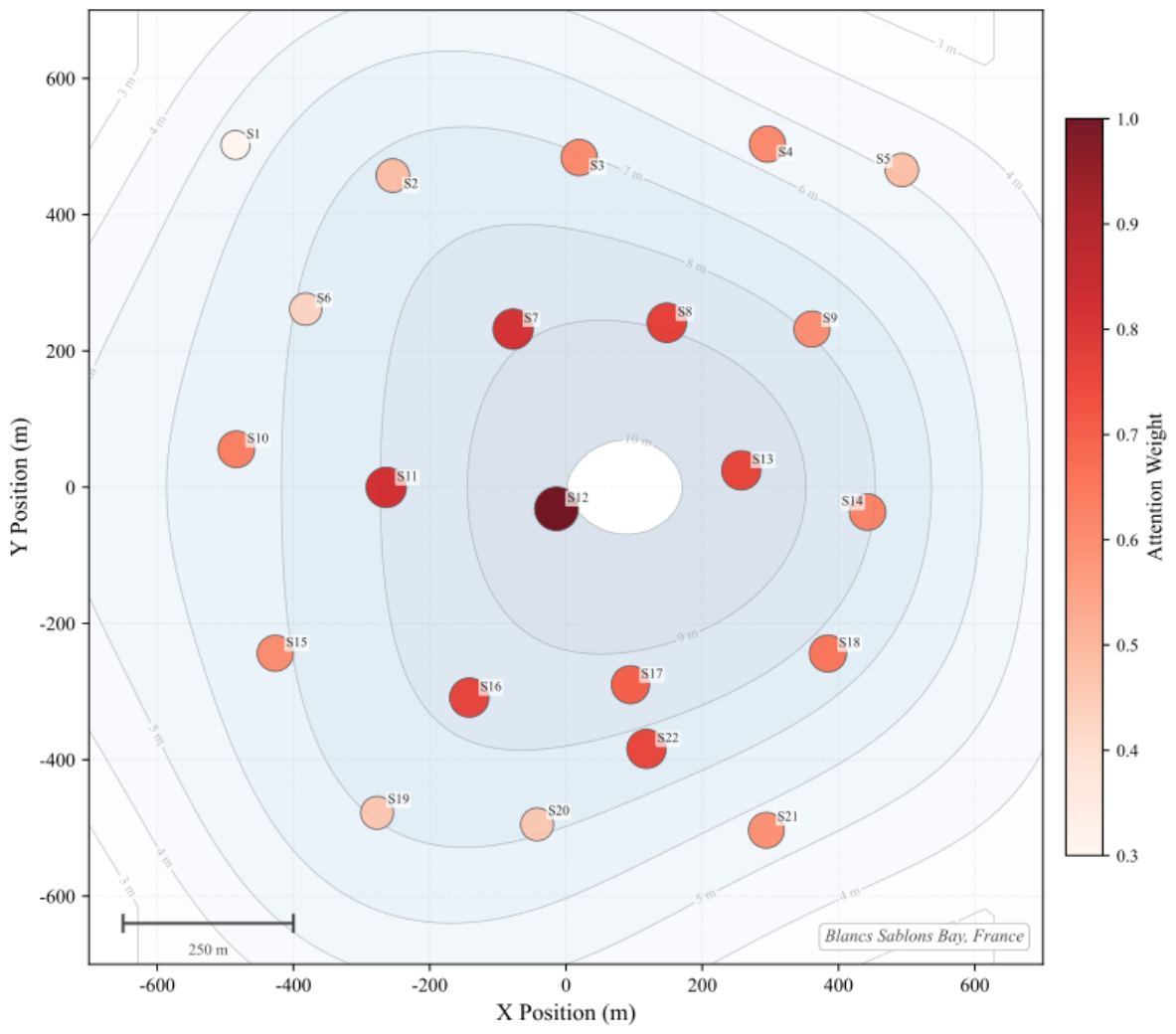
A total of 30 low-cost bottom pressure sensors were deployed with a sampling frequency of 2 Hz and a spacing of approximately 250 m, forming a multi-point observation network with distinct spatial distribution characteristics. During the approximately 4.2-month observation period, 22 sensors recorded complete data, while 5 sensors provided partial data due to battery failures or equipment anomalies, and 3 sensors failed to function. The 22 sensor stations with complete records were selected as experimental nodes. After preprocessing, including time drift correction and outlier removal, the observation data were used for model training and testing.

Considering the limited sample size of the original dataset, a data augmentation strategy was adopted to expand the training samples. Simulated wave signals under various sea conditions were generated based on the JONSWAP spectrum model.

Simulation parameters were set according to the statistical characteristics of the measured data, including a significant wave height range of 0.3 to 3.5 m, a peak period range of 4 to 12 s, and a wave direction coverage from northwest to southwest. Measurement noise with statistical properties similar to the actual data was superimposed on the simulated signals. Additionally, phase delays corresponding to the spatial layout of the sensor array were introduced to simulate the wave propagation process. The simulated data and actual data were mixed in a 7:3 ratio for model training, while the testing phase utilized only real-world data to evaluate the model’s generalization capability in authentic scenarios.

The experiment organizes training samples using a sliding time window approach, with a window length set to 256 sampling points (corresponding to an observation duration of 128 s). The prediction target is the current significant wave height ($H_s$). The dataset was partitioned chronologically into training, validation, and testing sets in a 7:1:2 ratio. Model training employed the Adam optimizer with an initial learning rate of 0.001, a batch size of 32, and a maximum of 200 training epochs, using an early stopping strategy to prevent overfitting. The number of parallel branches in the multi-scale graph convolutional network was set to 3, corresponding to feature aggregation from the first to third-order neighborhoods. The hidden state dimension was set to 64, and the number of Gated Recurrent Unit (GRU) layers was set to 2. All experiments were completed on a workstation equipped with an NVIDIA RTX 3090 GPU, and results were averaged over five independent runs to reduce the impact of randomness.

6.2. Evaluation Metrics and Comparison Methods

This study employs four indicators—Root Mean Square Error (RMSE), Mean Absolute Error (MAE), Mean Absolute Percentage Error (MAPE), and the Coefficient of Determination ($R^2$)—to evaluate wave height prediction performance. Let $y_i$ represent the observed wave height at the i-th time step, which is considered as the reference ground truth, and ${\widehat{y}}_i$ represent the corresponding predicted value. RMSE is defined as $RMSE=\sqrt{{\displaystyle \frac{1}{n}}{\sum }_{i=1}^n{(y_i-{\widehat{y}}_i)}^2}$, which reflects the overall deviation between predicted values and observations and is more sensitive to large errors, making it suitable for evaluating performance under extreme sea conditions. MAE is defined as $MAE={\displaystyle \frac{1}{n}}{\sum }_{i=1}^n|y_i-{\widehat{y}}_i|$, which characterizes the average magnitude of prediction errors and provides a robust measure of overall accuracy. MAPE is defined as $MAPE={\displaystyle \frac{1}{n}}{\sum }_{i=1}^n{\displaystyle \frac{|y_i-{\widehat{y}}_i|}{y_i}}\times 100\%$, which measures the relative error with respect to the observed wave height and reflects proportional deviations under different sea conditions, although it may become unstable when the wave height is small. The Coefficient of Determination is defined as $R^2=1-{\displaystyle \frac{{\sum }_{i=1}^n{(y_i-{\widehat{y}}_i)}^2}{{\sum }_{i=1}^n{(y_i-\overline{y})}^2}}$, which evaluates the model’s ability to explain variance and capture the variability of wave height.

To comprehensively evaluate the performance of the proposed method, several representative methods are selected as comparison baselines. The linear wave theory method [5] directly inverts pressure spectra to wave height spectra using a frequency domain transfer function; it is physically transparent but relies on stationarity assumptions and cannot adapt to non-stationary wave signals.

The multi-point averaging method computes a spatial average of pressure derived wave heights across all sensor nodes, which reduces random noise but discards inter-node phase and topological information. Long Short-Term Memory networks (LSTM) [22] model temporal dependencies through gated memory cells, enabling the capture of long-range sequence patterns, but operate on individual node time series without spatial structure awareness. LSTM-based architectures have been applied to wave parameter prediction tasks in several oceanographic studies, demonstrating their capability for short- to medium range forecasting of significant wave height from historical time series records. Gated Recurrent Units (GRU) [12] share a similar gated architecture to LSTM with a simplified structure, achieving comparable temporal modeling performance. Hao et al. [12] demonstrated the applicability of GRU networks to significant wave height prediction in the South China Sea, showing that the gated recurrent structure effectively captures the temporal evolution of wave conditions over multi-hour prediction horizons. One-dimensional Convolutional Neural Networks (1D-CNN) extract local temporal features through sliding convolution kernels but lack recurrent connections for long-term dependency modeling. Zhang et al. [13] combined CNN and LSTM components for wave height prediction and found that convolutional layers contribute to local feature extraction while the recurrent component handles temporal evolution, a hybrid strategy that has found increasing use in ocean wave forecasting. Graph Convolutional Networks (GCN) [7] extend the convolution operation to graph structured data through normalized adjacency-based neighborhood aggregation, enabling spatial topology-aware processing. Graph Attention Networks (GAT) [10] introduce a learnable attention mechanism into the neighborhood aggregation step, allowing adaptive weighting of neighboring nodes and improving the modeling of heterogeneous inter-node relationships. Spatio-Temporal Graph Convolutional Networks (STGCN) [4] combine graph convolution for spatial dependency modeling with temporal convolution or recurrent modules for sequence modeling, enabling joint spatio-temporal representation. All the aforementioned comparison methods adopt the same data partitioning and training strategies, and results reported for comparison methods are obtained by the authors under identical data splits and the same random seed conditions; hyperparameters for each method are optimized through grid search on the validation set.

6.3. Overall Performance Comparison

Table 1. Comparison of wave height prediction performance across different methods. All comparison method results were reproduced by the authors under the same data partitioning and random seed conditions. Hyperparameters are optimized via grid search on the validation set.

Method	RMSE (m)	MAE (m)	MAPE (%)	${\mathit{R}}^2$
Linear Wave Theory [2]	0.287	0.224	18.65	0.783
Multi-point Average	0.253	0.198	16.42	0.831
1 D-CNN	0.218	0.172	14.28	0.875
LSTM [22]	0.195	0.153	12.71	0.899
GRU [12]	0.189	0.148	12.35	0.906
GCN [3]	0.178	0.139	11.52	0.917
GAT [4]	0.169	0.132	10.87	0.925
STGCN [6]	0.158	0.123	10.15	0.934
Proposed Method	0.142	0.108	8.73	0.947

presents the comparative performance results of wave height prediction among the proposed method and various baseline approaches on the test set. It can be observed that traditional methods, including the linear wave theory and the multi-point averaging method, exhibit relatively low prediction accuracy, with RMSE values of 0.287 m and 0.253 m, respectively. This is mainly because these methods rely on simplified assumptions or local averaging strategies, and lack the ability to capture complex temporal dynamics and spatial interactions in wave signals.

Among the deep learning models, recurrent architectures such as LSTM and GRU outperform CNN, achieving lower RMSE values of 0.195 m and 0.189 m, respectively. This indicates that temporal dependency plays a critical role in wave height prediction. Compared with purely temporal models, graph-based methods (GCN and GAT) further improve performance by explicitly modeling spatial correlations between different measurement points. In particular, the GAT model achieves better performance than GCN due to its ability to adaptively learn the importance of neighboring nodes through attention mechanisms. The STGCN model further enhances prediction accuracy (RMSE = 0.158 m) by jointly modeling spatial and temporal dependencies. Building upon this, the proposed method achieves the best performance across all evaluation metrics, with an RMSE of 0.142 m, an MAE of 0.108 m, a MAPE of 8.73%, and an $R^2$ value of 0.947, demonstrating its superior capability in capturing complex spatio-temporal patterns of wave dynamics.

Table 1 demonstrates that the proposed spatio-temporal graph-based method achieves superior performance in wave height prediction. Compared with the linear wave theory method, the proposed method reduces the RMSE by 50.5%, and further achieves a 10.1% reduction compared with the STGCN model. This performance improvement can be attributed to the joint effect of adaptive adjacency matrix fusion, multi-scale graph convolution, and cross-dimensional attention mechanisms. Specifically, the adaptive adjacency matrix integrates the spatial configuration of sensors with dynamic signal correlations to construct a more flexible data-driven spatial representation; the multi-scale graph convolution captures spatial dependencies at different ranges; and the cross-dimensional attention mechanism enhances the interaction between spatial and temporal features. It is worth clarifying the relationship between this work and the original IFREMER observational study by Pineau-Guillou and Lazure [1]. The IFREMER work focuses on reporting and characterizing the quality and spatial correlation properties of the multi-sensor pressure dataset, representing a data-oriented observational contribution. The present study takes this dataset as the experimental basis and proposes a graph neural network-based wave height estimation framework that processes multi-node distributed signals jointly. The two works address different objectives and are complementary in nature; the present framework does not supersede the observational study but, rather, demonstrates how the spatial information contained in the distributed dataset can be more effectively exploited through graph-structured modeling.

6.4. Performance Analysis Under Different Sea States

The characteristics of ocean waves exhibit significant variations depending on the sea state conditions. To verify the adaptability of the proposed method across diverse sea states, the test data are categorized into three distinct classes based on the range of significant wave height ($H_s$) for analysis: low, medium, and high sea states. Low sea states correspond to calm sea conditions with a significant wave height of less than 1.0 m. Medium sea states correspond to general sea conditions where the significant wave height ranges between 1.0 and 2.0 m. High sea states correspond to harsh sea conditions with a significant wave height exceeding 2.0 m.

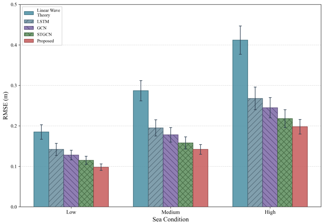
Figure 1 illustrates the comparison results of prediction errors for various methods across different sea state conditions. It can be observed from Figure 1 that the prediction errors for all methods are relatively small under low sea state conditions. This is because wave signal variations are comparatively gentle in low sea states, where the non-stationarity and non-linearity of the signals are weak. As the sea state level increases, the prediction errors of all methods show an upward trend; however, the proposed method exhibits the smallest increase in error. Under high sea state conditions, the RMSE of the linear wave theory method reaches $0.412$m, whereas that of the proposed method is only $0.198$m, highlighting a more pronounced performance advantage. This result indicates that the proposed method possesses superior adaptability across different sea state conditions, particularly in high sea states where it better captures the spatio-temporal evolution characteristics of complex wave fields. The widening performance gap in high sea states is attributed to the more prominent multi-scale characteristics of wave signals under harsh sea conditions. Wave components of different frequencies overlap to form complex spatio-temporal structures. The multi-scale graph convolutional structure of the proposed method can more effectively extract these multi-scale features, whereas traditional and single-scale methods encounter limitations when processing such complex signals.

6.5. Statistical Analysis of Prediction Error Characteristics

The statistical distribution characteristics of the prediction errors reflect the stability and reliability of the model’s prediction results. To conduct an in-depth analysis of the error distribution characteristics for each method, this study plots the probability density function (PDF) and cumulative distribution function (CDF) curves of the prediction errors.

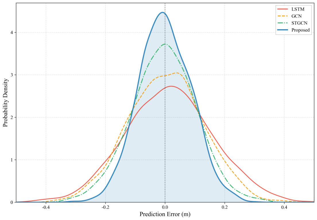
Figure 2 illustrates the probability density distribution of prediction errors for various deep learning methods. As observed in Figure 2, the error distribution curve of the proposed method is the sharpest, with its peak located near zero-error, indicating that the deviation between the predicted values and the ground truth is small and the distribution is concentrated. The error distribution of the LSTM method is relatively wide, exhibiting certain phenomena of both positive and negative biases. The error distribution characteristics of the GCN and STGCN methods are intermediate between those of LSTM and the proposed method; the introduction of graph structures improves the degree of concentration in the error distribution to some extent. The error distribution of the proposed method presents an approximately symmetric shape, with a comparable ratio of positive and negative biases, suggesting that the model does not possess a systematic tendency for overestimation or underestimation. This symmetric error distribution characteristic is of significant value for practical engineering applications, as it ensures the unbiasedness of the wave height estimation results. The concentration level of the error distribution reflects the stability of the model’s predictions. The narrow error distribution range of the proposed method indicates that its prediction performance maintains high consistency across different samples. This stability is primarily attributed to the dynamic adjustment capability of the graph structure enabled by the adaptive adjacency matrix fusion mechanism. The differences in error distribution shape among the methods can be understood from the perspective of their respective modeling capacities. The relatively wide and asymmetric error distribution of LSTM is associated with its inability to account for spatial dependencies across the sensor array; during periods of rapid sea state transition, single-node temporal models cannot simultaneously respond to the coherent changes occurring across multiple measurement stations, leading to concentrated residuals at transition peaks. The GCN and STGCN methods partially address this limitation by introducing graph-structured spatial modeling, and their narrower error distributions reflect the benefit of incorporating inter-node topological information. The proposed method’s error distribution is further concentrated toward zero through two complementary mechanisms: the adaptive adjacency matrix adjusts the graph structure at each time step to track the evolving wave propagation pattern, and the multi-scale graph convolution captures spatial coherence at multiple ranges simultaneously, reducing the prediction errors associated with both short-period wind–sea and long-period swell components.

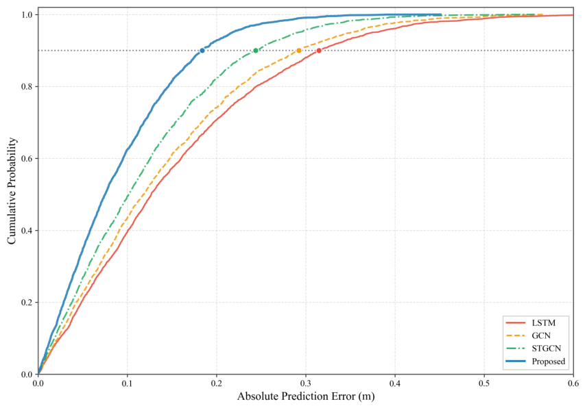
Figure 3 presents the Cumulative Distribution Function (CDF) of the absolute prediction errors for each method. The CDF intuitively reflects the sample coverage proportion under various error thresholds; a steeper curve indicates a higher proportion of samples with low errors. It is observed from Figure 3 that the proposed method’s CDF curve rises the most rapidly, covering approximately 80% of test samples at an error threshold of 0.15 m, whereas the LSTM method covers only about 55% under identical conditions. Regarding the error thresholds at the 90th percentile (90% cumulative probability), the proposed method achieves approximately 0.22 m, while STGCN, GCN, and LSTM reach 0.28 m, 0.34 m, and 0.38 m, respectively. This result further validates the proposed method’s superiority in controlling prediction errors, ensuring that the vast majority of samples maintain low error levels. The characteristics of the CDF are highly relevant for error boundary estimation in engineering applications and can be utilized to evaluate the accuracy range of wave height predictions at a specific confidence level.

6.6. Ablation Study Analysis

To evaluate the contributions of the key components within the proposed framework, an ablation study was conducted by systematically removing or replacing specific modules to analyze their impact on overall performance. Specifically, four variant models were established for comparative analysis: Variant A removes the adaptive adjacency matrix fusion mechanism and utilizes only a fixed adjacency matrix based on geometric distance; Variant B replaces the multi-scale graph convolution structure with a single-scale graph convolution; Variant C removes the gated temporal modeling module to evaluate the necessity of temporal dependency modeling; and Variant D removes the cross-dimensional attention fusion mechanism to assess its role in establishing spatio-temporal interaction pathways.

The ablation study results in

Table 2. Results of the ablation study.

Model Variant	RMSE (m)	MAE (m)	MAPE (%)	${\mathit{R}}^2$
Full Model	0.142	0.108	8.73	0.947
Variant A (No $A^{geo}$)	0.163	0.127	10.42	0.930
Variant B (Single-scale GCN)	0.156	0.121	9.87	0.936
Variant C (No Gated Temporal Modeling)	0.171	0.134	11.05	0.923
Variant D (No cross-dimensional attention)	0.152	0.118	9.65	0.939

demonstrate that each key component contributes to the overall performance of the model. As observed in Table 2, the removal of the gated temporal modeling module leads to the most significant performance decline, with the $RMSE$ increasing from $0.142$m to $0.171$m, representing a 20.4% increase. This highlights the critical role of temporal modeling in wave height prediction tasks, indicating that the temporal evolution patterns of wave signals are a key information source for achieving accurate predictions. Furthermore, after removing the adaptive adjacency matrix fusion mechanism, the RMSE rises to $0.163$m, suggesting that the dynamic graph structure is better suited to adapt to the time-varying characteristics of wave signals than a fixed graph structure. Replacing the multi-scale graph convolution with a single-scale version also results in a performance drop, verifying the necessity of multi-scale spatial feature extraction for capturing the multi-scale coherence characteristics of wave signals. While the performance decline after removing the cross-dimensional attention mechanism is relatively small, the degradation in metrics is still observable, illustrating that interaction learning between spatial and temporal features has a positive effect on enhancing the spatio-temporal fusion performance. Overall, these components achieve effective joint modeling of the spatio-temporal characteristics of distributed pressure sensing wave signals through their synergistic effects.

6.7. Multi-Scale Feature Weight Visualization Analysis

The multi-scale graph convolutional network adaptively fuses spatial features from different scales through an attention mechanism, where the weight allocation of each scale reflects the network’s degree of focus on information across various spatial ranges. To analyze the multi-scale feature fusion patterns learned by the network, this study provides a visualization of the scale attention weights under various sea state conditions.

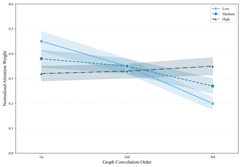
Figure 4 illustrates the attention weight distribution of multi-scale features across different sea state conditions. It can be observed from Figure 4 that under low sea state conditions, the network tends to assign larger weights to low-order graph convolutional features. Specifically, the average weights for 1st and 2nd order features are approximately $0.45$ and $0.35$, respectively, while the 3rd order feature weight is about $0.20$. This distribution pattern aligns with the physical characteristics of wave signals in low sea states. In calm sea conditions, waves are dominated by short-wave components with a smaller spatial coherence range; thus, information from low-order neighborhoods is more critical for wave height estimation. As the sea state level increases, the proportion of weights for high-order features gradually rises. Under high sea state conditions, the weight of 3rd order features increases to approximately $0.35$, approaching a uniform distribution across all scales. This trend indicates that the proportion of long-wave components increases in harsh sea conditions, resulting in a larger spatial coherence range that requires modeling with a broader scope of neighborhood information. Through the attention mechanism, the network automatically learns this multi-scale feature fusion strategy that varies with sea conditions, demonstrating the proposed method’s adaptive modeling capability relative to the physical characteristics of wave signals.

6.8. Analysis of the Adaptive Adjacency Matrix Fusion Coefficient

The adaptive adjacency matrix fusion mechanism integrates the geometric distance adjacency matrix (${\mathbf{A}}^{geo}$) and the signal correlation adjacency matrix (${\mathbf{A}}^{cor}$) using a learnable fusion coefficient $\alpha$. To investigate the learning behavior of the fusion coefficient, this study records its evolution trajectory during the training process and analyzes its statistical distribution across various sample conditions.

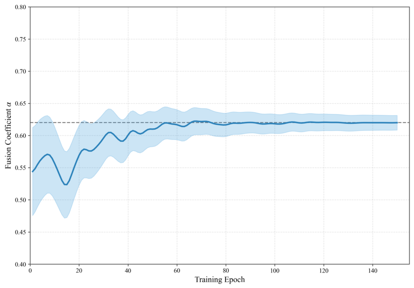
Figure 5 illustrates the convergence trajectory of the adjacency matrix fusion coefficient during the training process. As observed in Figure 5, the fusion coefficient exhibits significant fluctuations during the initial stages of training and gradually stabilizes as training progresses. After approximately 50 epochs, the fusion coefficient converges to around 0.62, indicating that the network tends to assign a slightly higher weight to the geometric distance adjacency matrix for this task. This result aligns with the physical background of wave measurement using distributed pressure sensing. The spatial deployment of sensors largely determines the signal correlation intensity between measurement points, while signal correlation provides dynamic supplementary information. The fact that the fusion coefficient does not converge to a boundary value 0 or 1 suggests that both types of adjacency matrices contribute to the wave height prediction task. Neither type of adjacency matrix alone can achieve optimal performance, which echoes the results of the ablation study. Furthermore, the standard deviation of the fusion coefficient gradually decreases during training, indicating that the coefficient tends to be consistent across different batches of samples, and the network has learned a stable graph structure fusion strategy.

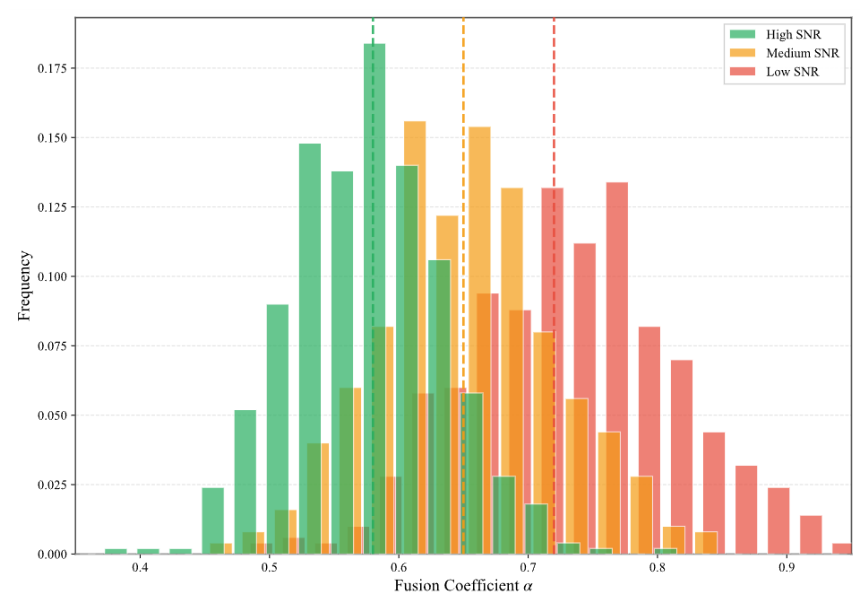
Figure 6 analyzes the statistical distribution of the fusion coefficients under different signal-to-noise ratio (SNR) conditions. It can be observed from Figure 6 that under high SNR conditions, the distribution of the fusion coefficients is relatively concentrated, with a mean value of approximately $0.58$, indicating a balanced utilization of both types of adjacency matrices when the signal quality is high. As the SNR decreases, the mean value of the fusion coefficient exhibits an upward trend, reaching approximately $0.72$ under low SNR conditions. This suggests that as signal quality degrades, the network relies more heavily on the stable geometric distance adjacency matrix (${\mathbf{A}}^{geo}$) while reducing the utilization of the noise-sensitive signal correlation adjacency matrix (${\mathbf{A}}^{cor}$). Such adaptive adjustment behavior reflects the robustness design of the fusion mechanism, which is capable of automatically selecting more reliable graph structure information sources based on the quality of the input data. This characteristic of the fusion coefficient distribution ensures that the proposed method maintains stable performance across varying levels of input data quality.

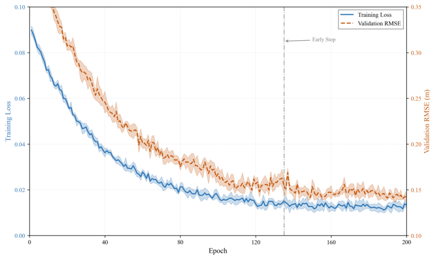
Regarding the convergence trajectory of the fusion coefficient shown in Figure 5, it is noted that $\alpha$ stabilizes after approximately 50 training epochs, and the validation set RMSE follows a broadly similar convergence pattern. Mild fluctuations in the validation RMSE become apparent after approximately epoch 80, reflecting a minor tendency toward overfitting at that stage. The early stopping mechanism monitors the validation RMSE and is triggered when no improvement is observed for 15 consecutive epochs, which in practice occurs at approximately epoch 120. The effective epoch range for reliable convergence in this experimental setting is therefore estimated to lie between 100 and 120 epochs. This range represents an empirical lower bound for the training duration rather than a strict stopping criterion, and the actual triggering point may vary modestly across different random initializations or dataset splits.

6.9. Sensitivity Analysis of Time Window Length

The time window length is a critical hyperparameter that significantly influences model performance. A shorter time window may fail to provide sufficient historical information, whereas an excessively long window might introduce redundant information and increase the computational burden. To analyze the impact of time window length on model performance, this study conducts comparative experiments under various window length settings.

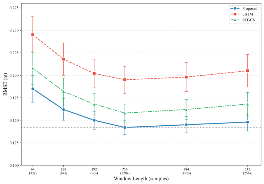
Figure 7 illustrates the variation trend of prediction error with respect to the time window length. It can be observed from Figure 7 that when the time window is too short, the prediction errors of all methods are relatively large; specifically, at a window length of 64 sampling points, the RMSE of the proposed method is approximately $0.185$m. As the window length increases, the prediction error gradually decreases, with the proposed method achieving optimal performance at a window length of 256 sampling points, yielding an $RMSE$ of $0.142$m. However, when the window length is further extended to 512 sampling points, the performance improvement does not continue, and the RMSE rises slightly to $0.148$m. This trend indicates that while a time window of appropriate length provides sufficient historical information for wave height prediction, the correlation between long-term historical data in excessively long windows and the current prediction target weakens, which may instead introduce interference into the prediction process. The proposed method outperforms the baseline methods across all window lengths, and its performance curve remains relatively flat, suggesting that the method possesses a certain degree of robustness to the time window length parameter. Furthermore, the selective memory mechanism of the Gated Recurrent Unit (GRU) enables the network to automatically filter out historical information irrelevant to the prediction task, thereby mitigating the information redundancy issues associated with long-term time windows to a certain extent.

6.10. Impact of Sensor Quantity on Prediction Performance

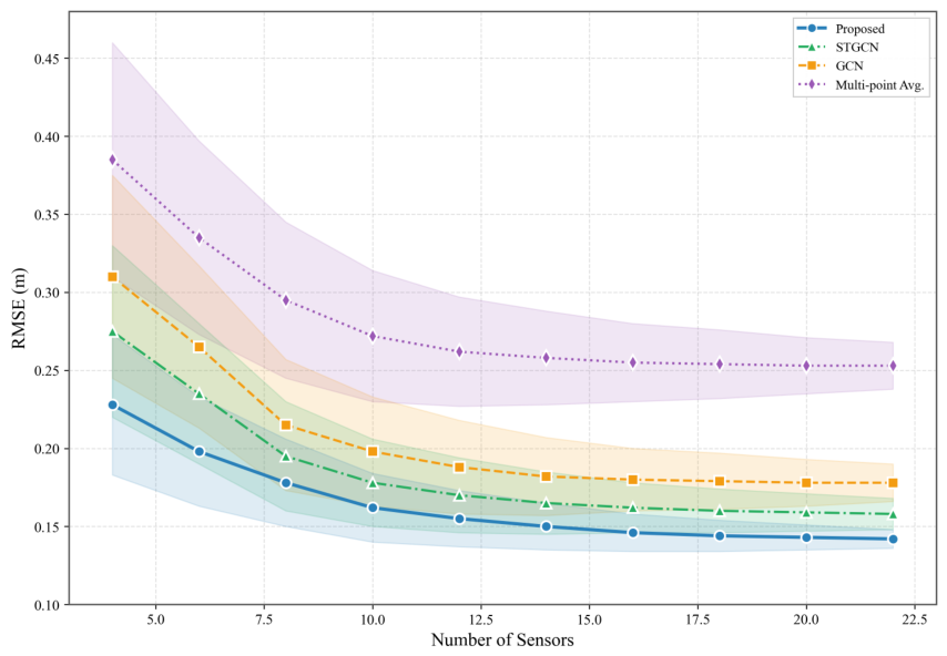
The number of nodes in a distributed sensing array is a critical factor influencing both the system cost and the observation density. To evaluate the impact of sensor quantity on wave height prediction performance, this study conducts prediction experiments by randomly selecting various subsets of sensors to construct the corresponding graph structures.

Figure 8 illustrates the variation in prediction performance with respect to the number of sensors. It can be observed from Figure 8 that when the number of sensors is small, the prediction errors for all methods are relatively high, accompanied by a wider range of fluctuations. This is because a limited number of sensors struggle to provide sufficient spatial sampling information to accurately characterize the spatial distribution characteristics of the wave field. As the number of sensors increases, the prediction error gradually decreases and tends to stabilize.

Examining the rate of change in the RMSE curves, the proposed method achieves a point of diminishing returns at approximately 10 sensors, beyond which additional sensors produce only marginal improvements in prediction accuracy. This reflects the spatial sampling density required to adequately represent the wave field structure at the scale of the Blancs Sablons Bay array. Under different deployment scenarios—for instance, arrays spanning larger geographic extents or monitoring longer-wavelength swell components—the minimum sensor count for stable performance may differ. The relatively favorable performance of the proposed method at low sensor counts, compared to GCN and STGCN, is primarily attributable to the adaptive graph construction mechanism, which constructs a more informative inter-sensor relationship representation even when the spatial sampling is sparse.

A comparison of the different methods reveals that the proposed method outperforms the baseline methods across all sensor quantity levels, with its advantage being more pronounced when the sensor count is low. Specifically, when the number of sensors is 8, the RMSE of the proposed method is approximately $0.178$m, whereas those of GCN and STGCN are approximately $0.215$m and $0.195$m, respectively. This result indicates that the adaptive graph structure construction and multi-scale feature fusion mechanisms of the proposed method can more effectively utilize the spatial information provided by limited sensors, demonstrating a clear advantage in application scenarios with constrained sensor deployment density.

6.11. Time-Series Visualization Analysis of Wave Height Prediction

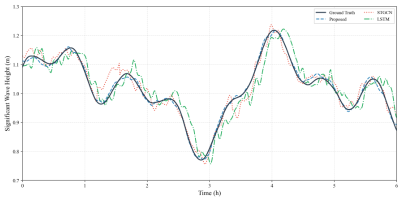
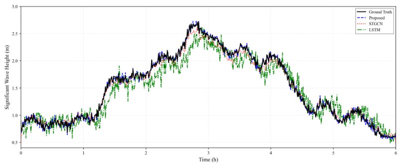
To provide an intuitive demonstration of the predictive performance of the proposed method, this study selects representative time segments from the test set for the visualization of time-series wave height prediction comparisons.

Figure 9 presents the time-series comparison of wave height prediction under calm sea conditions. It can be observed from Figure 9 that, during segments where the wave height changes relatively gradually, all methods are capable of effectively tracking the variation trends. The prediction curve of the proposed method demonstrates the highest degree of alignment with the ground truth. Conversely, the LSTM method exhibits a certain degree of phase lag, while the STGCN curve occasionally shows local deviations. Under calm sea conditions, the performance disparities among the methods are relatively minor, primarily reflected in the smoothness of the prediction curves and the accuracy of local peak and trough positions. The proposed method maintains high tracking precision during both gradual variations and local fluctuations, which is attributed to the effective capture of periodic signal characteristics by the gated temporal modeling module.

Figure 10 presents the time-series comparison of wave height prediction under changing sea conditions. It can be observed from Figure 10 that, during the phase where wave height rises rapidly, the LSTM method exhibits a significant lag bias, with the prediction error reaching its maximum as the wave height peaks. Although the tracking performance of the STGCN method is superior to that of LSTM, a certain degree of underestimation is still observable. The proposed method maintains high prediction accuracy throughout the entire variation process, demonstrating stronger responsiveness particularly near the turning points of rapid wave height changes. During the falling phase of wave height, while the prediction accuracy of all methods recovers to some extent, the advantage of the proposed method remains consistent. The prediction results under changing sea conditions validate the effectiveness of the proposed method in handling non-stationary wave signals. The multi-scale graph convolution structure and the adaptive adjacency matrix fusion mechanism enable the network to respond promptly to the spatio-temporal evolution of the wave field.

6.12. Scatter Plot Analysis of Predicted vs. True Values

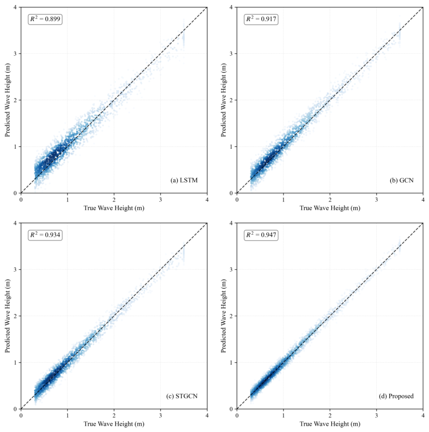
Scatter plots of predicted versus true values provide a comprehensive evaluation of the model’s performance across various wave height ranges, encompassing overall accuracy, local biases, and outlier distributions.

Figure 11 compares the prediction characteristics of different methods using scatter plots. As observed from Figure 11, the scatter distribution of the LSTM method is relatively dispersed, with a significant number of underestimated sample points in the high wave height region, yielding an $R^2$ value of $0.899$. Meanwhile, the GCN method shows an improved scatter distribution, certain deviations persist in both low and high wave height regions, with an $R^2$ value of $0.917$. The scatter points of the STGCN method are more concentrated around the ideal prediction line; however, some outliers are still observable under extreme conditions where wave heights exceed $2.5$m, resulting in an $R^2$ value of $0.934$. In contrast, the proposed method exhibits the most concentrated scatter distribution, maintaining high prediction accuracy across the entire wave height range with very few samples significantly deviating from the ideal prediction line, achieving an $R^2$ value of $0.947$. The distribution characteristics of the scatter plots indicate that the proposed method possesses stable predictive capabilities across various wave height intervals, without systematic bias toward specific ranges. This consistency is of great significance for full-range wave height estimation in practical engineering applications.

6.13. Performance Analysis Across Different Wave Frequency Bands

Ocean waves are typically composed of the superposition of multiple frequency components, with wave components in different frequency bands contributing differently to the significant wave height ($H_s$). To analyze the modeling capability of the proposed method for wave components across various frequency bands, this study performs spectral analysis on the test data. The wave signals are decomposed into swell and wind–sea components to evaluate the prediction performance of each method under these two distinct wave categories respectively.

Figure 12 compares the prediction performance of various methods under swell-dominated and wind-sea-dominated conditions. It can be observed from Figure 12 that most methods exhibit higher prediction errors under wind-sea-dominated conditions compared to swell-dominated ones. This is because wind–sea waves are characterized by higher frequencies and smaller spatial coherence scales, leading to more intense spatio-temporal variations that impose higher demands on the model’s modeling capability.

The LSTM method shows a significant performance gap between the two conditions, with an RMSE of approximately 0.175 m for swell-dominated conditions, which rises to 0.228 m for wind–sea-dominated conditions. In contrast, the proposed method maintains lower prediction errors in both scenarios, with RMSE values of approximately 0.132 m and 0.158 m for swell and wind–sea dominated conditions, respectively, representing a relatively smaller performance disparity. This result demonstrates that the multi-scale graph convolution structure of the proposed method can adapt to the spatial coherence characteristics of wave components in different frequency bands. Specifically, the low-order graph convolution branches play a more significant role when processing short-period wind–sea, while the contribution of high-order branches increases when handling long-period swell, thereby achieving balanced modeling of waves across different frequency bands.

6.14. Analysis of Model Training Convergence Process

The training convergence characteristics of a model reflect the stability and efficiency of its learning process. To analyze the training behavior of the proposed method, this study records the evolution curves of the loss function and validation set performance metrics throughout the entire training phase.

Figure 13 illustrates the convergence curves of the training loss and the validation set RMSE during the training process. It can be observed from Figure 13 that the training loss decreases rapidly within the first 50 epochs, subsequently entering a slow descent phase and stabilizing at approximately the 120th epoch. The variation trend of the validation set RMSE is similar to that of the training loss; however, slight fluctuations occur after the 80th epoch, indicating a minor overfitting tendency in the model during this stage.

The early stopping mechanism is triggered when the validation set RMSE fails to improve for 15 consecutive epochs, and the model parameters with the optimal performance on the validation set are ultimately selected for testing. Based on the observed convergence trajectories, the effective training duration for this experimental setting falls in the range of approximately 100 to 120 epochs, as the fusion coefficient stabilizes after epoch 50 and the early stopping criterion is satisfied at approximately epoch 120. This range serves as an empirical reference for training configuration rather than a fixed requirement; in practice, monitoring the validation set metric and applying the early stopping criterion as described above provides a reliable basis for determining when to terminate training The convergence curves of the training process demonstrate that the proposed method possesses excellent training stability, characterized by a smooth and continuous decline in the loss function without severe oscillations or divergence. Furthermore, the small standard deviation across five independent experiments suggests that the model is insensitive to random initialization and can stably converge to a consistent performance level.

6.15. Node Attention Weight Visualization

The graph-level readout in the output layer utilizes an attention pooling mechanism to aggregate node features, where the attention weights assigned to the nodes reflect the contribution levels of individual sensors to the wave height prediction task. To investigate the node importance distribution learned by the network, this study projects the attention weights onto the spatial coordinates of the sensor array for visualization.

Figure 14 illustrates the spatial distribution of sensor node attention weights. It can be observed from Figure 14 that the node importance learned by the network exhibits a clear spatial distribution pattern: sensor nodes located in the central region of the array generally obtain higher attention weights, whereas the weights of sensors in the peripheral areas are relatively lower. This distribution pattern is correlated with the spatial observation characteristics of the wave field. Specifically, sensors in the central region can receive information from neighboring nodes in all directions, making their feature representations more representative and contributing more significantly to the overall wave height estimation.

Furthermore, some sensor nodes located in deeper water also obtain relatively higher weights. This may be attributed to the fact that pressure signals in deep-water areas are less affected by seabed topography, resulting in higher signal quality. The visualization results of the node weight distribution provide a valuable reference for the deployment optimization of sensor arrays. In practical applications, the spatial configuration of sensors can be adjusted based on the learned node importance distribution to enhance overall measurement efficiency.

7. Conclusions and Future Work

The graph construction method proposed in this study represents the inter-sensor relationships through a combination of geometric distance and signal correlation, which encodes physical environmental information in an implicit rather than explicit manner. This approach provides flexibility and adaptability to time-varying wave propagation patterns but carries limitations when the seafloor topographic relief is pronounced or when wave energy pathways are substantially constrained by local bathymetric features. Future research will explore the explicit incorporation of physical environmental parameters—including water depth fields, seafloor topographic gradients, distance from the shoreline, prevailing wave propagation directions, and bottom sediment composition and physical properties—into the graph structure, either as node-level features or as physically informed edge weights. In addition, hybrid modeling strategies that couple data-driven graph representations with physics-based wave propagation constraints will be investigated, with the goal of further improving robustness under complex bathymetric conditions and diverse sea state regimes. The scalability of the proposed framework within larger scale sensor networks and its applicability to open-ocean deployment scenarios also constitute important directions for future investigation. Future research will also explore the scalability of the model within larger-scale sensor networks and investigate hybrid modeling strategies that incorporate physical constraints to further enhance robustness.

References

1. Pineau-Guillou, L.; Lazure, P. A high-frequency dataset of sea level observations from low-cost pressure sensors. Sci. Data 2025, 12, 999. [Google Scholar] [CrossRef] [Scilit] [PubMed]
2. Rossi, G.B.; Cannata, A.; Iengo, A.; Migliaccio, M.; Nardone, G.; Piscopo, V.; Zambianchi, E. Measurement of sea waves. Sensors 2021, 22, 78. [Google Scholar] [CrossRef] [Scilit]
3. Khemani, B.; Patil, S.; Kotecha, K.; Tanwar, S. A review of graph neural networks: Concepts, architectures, techniques, challenges, datasets, applications, and future directions. J. Big Data 2024, 11, 18. [Google Scholar] [CrossRef] [Scilit]
4. Dong, G.; Tang, M.; Wang, Z.; Gao, J.; Guo, S.; Cai, L.; Gutierrez, R.; Campbel, B.; Barnes, L.E.; Boukhechba, M. Graph neural networks in IoT: A survey. ACM Trans. Sens. Netw. 2023, 19, 47. [Google Scholar] [CrossRef] [Scilit]
5. Jin, G.; Liang, Y.; Fang, Y.; Shao, Z.; Huang, J.; Zhang, J.; Zheng, Y. Spatio-temporal graph neural networks for predictive learning in urban computing: A survey. IEEE Trans. Knowl. Data Eng. 2023, 36, 5388–5408. [Google Scholar] [CrossRef] [Scilit]
6. Jiang, W.; Luo, J. Graph neural network for traffic forecasting: A survey. Expert Syst. Appl. 2022, 207, 117921. [Google Scholar] [CrossRef] [Scilit]
7. Lu, T.; Wang, Y.P.; Quan, Q.; Gao, C.; Gao, S. Wave heights from sea surface and bottom measurements: Variations with different water depths. Ocean Eng. 2023, 287, 115848. [Google Scholar] [CrossRef] [Scilit]
8. Lyman, T.P.; Elsmore, K.; Gaylord, B.; Byrnes, J.E.; Miller, L.P. Open Wave Height Logger: An open source pressure sensor data logger for wave measurement. Limnol. Oceanogr. Methods 2020, 18, 335–345. [Google Scholar] [CrossRef] [Scilit]
9. Yin, X.; Wu, T.; Yu, J.; He, X.; Xu, L. A significant wave height prediction method with ocean characteristics fusion and spatiotemporal dynamic graph modeling. Acta Oceanol. Sin. 2024, 43, 13–33. [Google Scholar] [CrossRef] [Scilit]
10. Glover, H.; Wengrove, M.; Holman, R. Measuring hydrodynamics and exploring nearshore processes using distributed sensing of fiber-optic cable strain. Coast. Eng. 2024, 190, 104487. [Google Scholar] [CrossRef] [Scilit]
11. Höttges, A.; Smaadahl, M.; Evers, F.M.; Boes, R.M.; Rabaiotti, C. Dynamic wave measurement with a high spatial resolution distributed fiber optic pressure sensor. IEEE Sens. J. 2024, 24, 22387–22396. [Google Scholar] [CrossRef] [Scilit]
12. Hao, P.; Li, S.; Gao, Y. Significant wave height prediction based on deep learning in the South China Sea. Front. Mar. Sci. 2023, 9, 1113788. [Google Scholar] [CrossRef] [Scilit]
13. Zhang, J.; Luo, F.; Quan, X.; Wang, Y.; Shi, J.; Shen, C.; Zhang, C. Improving wave height prediction accuracy with deep learning. Ocean Model. 2024, 188, 102312. [Google Scholar] [CrossRef] [Scilit]
14. Vrahatis, A.G.; Lazaros, K.; Kotsiantis, S. Graph attention networks: A comprehensive review of methods and applications. Future Internet 2024, 16, 318. [Google Scholar] [CrossRef] [Scilit]
15. Li, Z.L.; Zhang, G.W.; Yu, J.; Xu, L.Y. Dynamic graph structure learning for multivariate time series forecasting. Pattern Recognit. 2023, 138, 109423. [Google Scholar] [CrossRef] [Scilit]
16. Sun, Y.; Jiang, X.; Hu, Y.; Duan, F.; Guo, K.; Wang, B.; Gao, J.; Yin, B. Dual dynamic spatial-temporal graph convolution network for traffic prediction. IEEE Trans. Intell. Transp. Syst. 2022, 23, 23680–23693. [Google Scholar] [CrossRef] [Scilit]
17. Leng, J.; Gao, M.; Gong, H.; Chen, B.; Zhou, C.; Shi, M.; Chen, Z.; Li, X. Spatio-temporal prediction of regional land subsidence via ConvLSTM. J. Geogr. Sci. 2023, 33, 2131–2156. [Google Scholar] [CrossRef] [Scilit]
18. Chen, Z.; Lu, Z.; Chen, Q.; Zhong, H.; Zhang, Y.; Xue, J.; Wu, C. Spatial–temporal short-term traffic flow prediction model based on dynamical-learning graph convolution mechanism. Inf. Sci. 2022, 611, 522–539. [Google Scholar] [CrossRef] [Scilit]
19. Liu, Y.; Guo, B.; Meng, J.; Zhang, D.; Yu, Z. Spatio-temporal memory augmented multi-level attention network for traffic prediction. IEEE Trans. Knowl. Data Eng. 2023, 36, 2643–2658. [Google Scholar] [CrossRef] [Scilit]
20. Elizar, E.; Zulkifley, M.A.; Muharar, R.; Zaman, M.H.M.; Mustaza, S.M. A review on multiscale-deep-learning applications. Sensors 2022, 22, 7384. [Google Scholar] [CrossRef] [Scilit]
21. Ding, C.; Sun, S.; Zhao, J. MST-GAT: A multimodal spatial–temporal graph attention network for time series anomaly detection. Inf. Fusion 2023, 89, 527–536. [Google Scholar] [CrossRef] [Scilit]
22. Hochreiter, S.; Schmidhuber, J. Long short-term memory. Neural Comput. 1997, 9, 1735–1780. [Google Scholar] [CrossRef] [Scilit] [PubMed]
Figure 1. Comparison of Prediction Errors of Different Methods under Various Sea Conditions. The horizontal axis denotes the sea state categories, while the vertical axis represents RMSE in meters (m). Grouped bar charts with distinct colors represent Linear Wave Theory, LSTM, GCN, STGCN, and the proposed method, respectively. Error bars depict the standard deviation range over five independent experiments. The sea state categories are defined based on the significant wave height ( H s ): low sea state ( H s < 1.0 m), medium sea state (1.0 m H s 2.0 m), and high sea state ( H s > 2.0 m).
Applsci 16 04073 g001
Figure 2. Probability Density Distribution of Prediction Errors for Different Methods. The horizontal axis represents the prediction error in meters (m), where positive values denote overestimation and negative values denote underestimation. The vertical axis represents the probability density. Curves of different colors correspond to LSTM, GCN, STGCN, and the proposed method, respectively. The dashed line indicates the zero-error position. A distribution that is more concentrated near the zero point indicates higher prediction accuracy.
Applsci 16 04073 g002
Figure 3. Cumulative Distribution Function (CDF) of prediction errors. The horizontal axis represents the absolute value of the prediction error in meters (m). The vertical axis represents the cumulative probability. Curves of different colors correspond to LSTM, GCN, STGCN, and the proposed method, respectively. The horizontal dashed line marks the position corresponding to the 90% cumulative probability. A steeper upward slope of the curve indicates a higher proportion of samples with small errors.
Applsci 16 04073 g003
Figure 4. Distribution of multi-scale feature attention weights across different sea state conditions. The horizontal axis denotes the graph convolution order, corresponding to different spatial receptive field ranges: the 1st, 2nd, and 3rd orders represent 1-hop, 2-hop, and 3-hop neighborhoods, respectively. The vertical axis represents the normalized attention weights. Curves of distinct colors correspond to low, medium, and high sea state conditions. The shaded error bands depict the distribution range of weights for different samples under the same sea state category.
Applsci 16 04073 g004
Figure 5. Training convergence process of the adjacency matrix fusion coefficient. The horizontal axis represents the number of training epochs, and the vertical axis represents the value of the fusion coefficient α , ranging from 0 to 1. An α value approaching 1 indicates that the geometric distance adjacency matrix is dominant, whereas an α value approaching 0 indicates that the signal correlation adjacency matrix is dominant. The solid line denotes the mean value of the fusion coefficient on the training set, and the shaded area represents the standard deviation range. The dashed line marks the stable value after convergence.
Applsci 16 04073 g005
Figure 6. Distribution of fusion coefficients under different signal-to-noise ratio (SNR) conditions. The horizontal axis represents the values of the fusion coefficient α , while the vertical axis represents the frequency distribution. Histograms of different colors correspond to high SNR, medium SNR, and low SNR conditions, respectively. The SNR is estimated based on the power spectral characteristics of the pressure signals. Dashed lines mark the mean positions of the fusion coefficients for each condition.
Applsci 16 04073 g006
Figure 7. Trend of prediction error versus time window length. The horizontal axis represents the time window length in sampling points, with the corresponding duration in parentheses. The vertical axis represents RMSE in meters (m). The solid line denotes the proposed method, while the dashed lines represent the LSTM and STGCN methods, respectively. Error bars indicate the standard deviation from five independent experiments. The horizontal dot-dashed line marks the optimal performance level achieved by the proposed method.
Applsci 16 04073 g007
Figure 8. Relationship between prediction performance and the number of sensors. The horizontal axis represents the number of sensors involved in modeling. The vertical axis represents the RMSE in meters. Curves of different colors correspond to the proposed method, STGCN, GCN, and the multi-point averaging method, respectively. The shaded areas indicate the range of performance fluctuations under different sensor combinations. For each quantity level, experiments were conducted by randomly selecting 10 different sensor combinations.
Applsci 16 04073 g008
Figure 9. Time-series comparison of wave height prediction under calm sea conditions. The horizontal axis represents time in hours (h), while the vertical axis represents the significant wave height in meters (m). The black solid line denotes the ground truth wave height, the blue dashed line represents the predicted values of the proposed method, the red dotted line indicates the predictions of STGCN, and the green dash-dotted line shows the predictions of LSTM. This time segment corresponds to the calm sea conditions in the test set, where the significant wave height fluctuates within the range of 0.8 to 1.2 m.
Applsci 16 04073 g009
Figure 10. Time-series comparison of wave height prediction under changing sea conditions. The horizontal axis represents time in hours (h), while the vertical axis represents the significant wave height in meters (m). The black solid line denotes the ground truth wave height, the blue dashed line represents the predicted values of the proposed method, the red dotted line indicates the predictions of STGCN, and the green dash-dotted line shows the predictions of LSTM. This time interval covers the transition of sea conditions from calm to rough and then back to moderate, with the significant wave height varying within the range of 0.6 to 2.8 m.
Applsci 16 04073 g010
Figure 11. Comparison of scatter plots between predicted and ground truth values for different methods. The horizontal axis represents the ground truth wave height, and the vertical axis represents the predicted wave height, both measured in meters. The four subplots correspond to LSTM, GCN, STGCN, and the proposed method, respectively. The black dashed diagonal line represents the ideal prediction line ( y = x ). The color intensity of the scatter points indicates the sample density, with darker colors representing a higher concentration of samples in that region. The R 2 values (coefficient of determination) for each method are annotated in the respective plots.
Applsci 16 04073 g011
Figure 12. Comparison of predictive performance under swell-dominated and wind–wave-dominated conditions. The horizontal axis represents the method category, and the vertical axis indicates the RMSE(m). Blue bars denote prediction errors for swell-dominated conditions, while orange bars represent wind–wave-dominated conditions. Error bars signify the standard deviation. Swell-dominated conditions are defined by a peak period exceeding 8 s, and wind–wave-dominated conditions by a peak period under 6 s.
Applsci 16 04073 g012
Figure 13. Convergence curves of training loss and validation set RMSE. The horizontal axis represents the number of training epochs. The left vertical axis represents the training loss, while the right vertical axis denotes the validation set RMSE in meters (m). The blue solid line represents the training loss, and the orange dashed line represents the validation set RMSE. The shaded areas indicate the standard deviation range across five independent experiments. The vertical dash-dotted line marks the position where the early stopping mechanism was triggered.
Applsci 16 04073 g013
Figure 14. Spatial distribution of sensor node attention weights. The dots in the figure represent sensor positions, where the size and color intensity of each dot indicate the node’s attention weight; a larger dot and darker color signify a greater weight. The coordinate axes denote the spatial positions of the sensors relative to the center of the array, measured in meters (m). The background contour lines illustrate the approximate water depth distribution in the region, with values in meters (m). The attention weights represent the mean values calculated over the test set.
Applsci 16 04073 g014