Multi-Scale Atrous Feature Fusion Based on a VGG19-UNet Encoder for Brain Tumor Segmentation

Abstract

Accurate brain tumor segmentation from magnetic resonance imaging (MRI) remains challenging due to heterogeneous tumor morphology, intensity variability, and multi-scale structural complexity. This study proposes a DeepLabV3+-based segmentation framework integrating a VGG19-UNet encoder, Atrous Spatial Pyramid Pooling (ASPP), and low-level feature refinement to simultaneously capture hierarchical semantics and boundary-sensitive spatial details. The architecture enhances receptive field coverage without additional downsampling while preserving fine-grained contour information during reconstruction. Extensive evaluation was conducted on the Figshare Brain Tumor Segmentation (FBTS) dataset and the BraTS 2021 and BraTS 2018 benchmarks, focusing on Whole Tumor segmentation across multiple MRI modalities and tumor grades. Under five-fold cross-validation, the proposed model achieved a mean Dice Similarity Coefficient of 0.9717 and Jaccard Index of 0.9456 on FBTS, with stable and competitive performance across FLAIR, T1, T2, and T1CE modalities in both HGG and LGG cases. Boundary-level analysis further confirmed controlled Hausdorff Distance and low Average Symmetric Surface Distance. Statistical validation and ablation analysis demonstrate consistent improvements over baseline U-Net configurations. The proposed framework provides a robust and computationally efficient solution for automated brain tumor segmentation across heterogeneous datasets.

1. Introduction

Brain tumor segmentation from magnetic resonance imaging (MRI) is a fundamental component of clinical workflows, supporting diagnosis, surgical planning, radiotherapy targeting, and longitudinal disease monitoring [1,2,3]. Accurate delineation of tumor boundaries enables quantitative assessment of tumor volume, growth rate, and treatment response [4]. However, manual segmentation remains time-consuming, labor-intensive, and subject to inter-observer variability [5,6]. These limitations motivate the development of automated and reliable segmentation frameworks.

Despite significant advances in deep learning, automated brain tumor segmentation remains challenging [7]. Tumors exhibit substantial heterogeneity in size, shape, texture, and intensity distribution across patients [3,8]. Infiltrative tumor margins often appear diffuse and poorly defined, particularly in glioma cases [9]. Moreover, MRI scans frequently contain noise artifacts, partial volume effects, and acquisition variability across scanners and imaging protocols [10]. From a modeling perspective, these factors require segmentation architectures capable of simultaneously capturing large-scale contextual dependencies and preserving fine-grained spatial details. Achieving this balance between global semantic abstraction and local boundary precision remains a non-trivial problem.

Encoder–decoder convolutional neural networks have become the dominant paradigm for biomedical segmentation [11,12]. The introduction of U-Net [13] established a powerful symmetric architecture that integrates deep semantic features with high-resolution spatial information via skip connections. Numerous extensions have been proposed, including residual U-Net, attention-based U-Net, and densely connected variants [14,15,16,17,18]. While these approaches improve gradient flow and feature refinement, conventional U-Net architectures are inherently constrained by their receptive field size. As a result, modeling long-range spatial dependencies and large tumor structures may remain suboptimal.

To enhance global context modeling, multi-scale representation strategies have been introduced. Atrous (dilated) convolution expands the receptive field without reducing spatial resolution or increasing parameter count. DeepLab-based models incorporate Atrous Spatial Pyramid Pooling (ASPP) to aggregate multi-scale contextual features at different dilation rates [15,16,19,20]. Although such architectures demonstrate strong semantic representation capability, their simplified decoder structures may lead to insufficient boundary refinement, particularly in medical imaging tasks where precise delineation is critical.

Another line of research integrates pretrained classification backbones into segmentation frameworks. Networks such as VGG and ResNet have been embedded into U-Net architectures to leverage hierarchical feature representations learned from large-scale natural image datasets [7,21]. Pretrained encoders often improve convergence stability and generalization in limited medical datasets [22,23]. However, existing VGG-based U-Net implementations typically rely on standard symmetric decoders and do not explicitly incorporate advanced multi-scale context modeling modules [24]. Conversely, DeepLab-style models emphasize context aggregation, but do not fully exploit intermediate hierarchical representations for boundary-sensitive refinement [16].

Recent advancements in Transformer-based and state-space models have shown promising results in capturing long-range dependencies through self-attention and sequence modeling mechanisms [25]. Architectures such as TransUNet [26,27], Swin-UNet [28,29], and emerging Mamba-based models [30,31] enable improved global context representation; however, their increased computational complexity and reliance on large-scale training data remain challenging for practical medical imaging applications, particularly in scenarios requiring precise boundary delineation and efficiency.

Therefore, a methodological gap persists: achieving an effective architectural integration that simultaneously (i) enlarges the receptive field to model heterogeneous tumor context, (ii) preserves intermediate spatial representations for boundary accuracy, and (iii) maintains computational efficiency suitable for practical deployment. Existing models tend to prioritize either contextual abstraction or spatial detail, but rarely optimize both in a unified and explicitly structured manner.

To address this gap, we propose a Multi-Scale Atrous Feature Fusion framework grounded in a VGG19-UNet encoder architecture. The proposed method first constructs a VGG19-UNet to expose hierarchical encoder feature maps across multiple representation depths. Deep semantic representations extracted from the encoder bottleneck are enhanced using an Atrous Spatial Pyramid Pooling (ASPP) module to capture multi-scale contextual dependencies without additional downsampling. In parallel, intermediate encoder features are projected through a lightweight low-level feature (LLF) refinement branch to preserve boundary-sensitive spatial information. Unlike conventional symmetric decoder designs, the proposed architecture restructures the segmentation head by explicitly fusing ASPP-enhanced global features with refined intermediate representations, followed by compact convolutional refinement and full-resolution reconstruction. This decoupled design enables the network to balance receptive field expansion and spatial precision within a computationally efficient framework. By leveraging hierarchical encoder representations rather than relying solely on standard decoder pathways, the proposed approach differentiates itself from both classical U-Net variants and DeepLab-based segmentation models.

The main contributions of this work are summarized as follows:

• We construct a VGG19-UNet encoder framework that exposes hierarchical multi-level feature representations tailored for brain tumor segmentation.
• We integrate an Atrous Spatial Pyramid Pooling module at the encoder bottleneck to enhance multi-scale contextual modeling without excessive parameter growth.
• We introduce a low-level feature refinement branch that preserves intermediate spatial information and improves tumor boundary delineation.
• We propose a structured feature fusion mechanism that explicitly balances global semantic abstraction and spatial detail preservation within a compact reconstruction head.
• We conduct a comprehensive experimental evaluation, including ablation studies, cross-dataset validation, and statistical analysis, to demonstrate the effectiveness and robustness of the proposed architecture.

The remainder of this paper is organized as follows. Section 2 reviews related work in convolutional neural network-based brain tumor segmentation, pretrained encoder integration, and multi-scale context modeling. Section 3 describes the datasets, the preprocessing procedures and the detailed architecture of the proposed method. Section 4 presents the experimental setup and quantitative results, including ablation and statistical analyses. Section 5 discusses the findings, computational efficiency considerations, limitations, and clinical implications. Finally, Section 6 concludes the paper and outlines directions for future research.

2. Related Work

This section reviews existing approaches to brain tumor segmentation, with emphasis on encoder–decoder architectures, pretrained backbone integration, and multi-scale context modeling. We analyze methodological limitations to highlight the research gap addressed by the proposed framework.

2.1. Encoder–Decoder CNN Architectures

Encoder–decoder convolutional neural networks represent the dominant paradigm in medical image segmentation. U-Net [13] introduced symmetric skip connections that merge low-level spatial features with deep semantic representations, enabling precise localization. Subsequent extensions, including residual U-Net, dense U-Net, and attention U-Net [14,15,16,17,18], have focused on improving gradient flow, feature reuse, and adaptive weighting of salient regions.

Despite these improvements, conventional U-Net architectures exhibit two structural limitations. First, progressive downsampling reduces spatial resolution and limits the effective receptive field, potentially hindering accurate modeling of large or heterogeneous tumor structures [32]. Second, contextual modeling is implicitly achieved through stacked convolutions rather than explicitly designed multi-scale mechanisms [33,34]. As a result, the balance between global semantic abstraction and boundary precision remains suboptimal.

2.2. Pretrained Encoder-Based U-Net Variants

To improve feature robustness and generalization, pretrained classification backbones such as VGG, ResNet, and EfficientNet have been incorporated into U-Net frameworks [35,36,37]. Pretraining on large-scale natural image datasets improves convergence stability and strengthens hierarchical representation learning.

However, most pretrained U-Net variants retain the conventional symmetric decoder without structural modification [34]. While the encoder becomes more powerful, the architecture does not fundamentally expand its receptive field beyond the inherent convolutional depth [38,39]. Consequently, pretrained VGG-based U-Net models improve representation robustness but do not explicitly address multi-scale contextual dependency modeling [40]. Furthermore, decoder pathways remain heavy and symmetric, potentially increasing computational overhead without proportional gains in context awareness [41].

2.3. Multi-Scale Context Modeling and DeepLab-Based Approaches

Multi-scale representation strategies have been widely explored to overcome limited receptive field constraints. Atrous convolution enlarges the receptive field while maintaining spatial resolution. DeepLab-based architectures incorporate Atrous Spatial Pyramid Pooling (ASPP) to aggregate contextual information at multiple dilation rates [20,42]. Feature Pyramid Networks (FPN) and pyramid pooling modules similarly aim to integrate hierarchical multi-scale cues [16,43,44].

Although DeepLab-style models demonstrate strong performance in natural image segmentation [42,45], their direct application to medical imaging presents challenges. First, simplified decoder structures may inadequately recover fine tumor boundaries, which are critical in clinical practice. Second, aggressive multi-scale aggregation may oversmooth small tumor subregions. Third, some multi-scale frameworks significantly increase computational complexity, limiting their practicality in resource-constrained environments [1,46,47].

2.4. Hybrid Multi-Scale and Boundary-Aware Segmentation Models

Recent studies attempt to combine context modeling with boundary refinement mechanisms. Attention-based multi-scale networks and dual-branch architectures have been proposed to capture complementary features [17,48]. However, many of these designs introduce additional parameters or complex attention modules, increasing the size of the model and the training instability [48,49]. Moreover, the integration of multi-scale modules with pretrained encoder hierarchies is often performed without explicitly leveraging intermediate feature representations for structured fusion.

2.5. Transformer and State-Space-Based Segmentation Models

Recent advances in medical image segmentation have increasingly explored Transformer-based architectures to address the limitations of convolutional neural networks in modeling long-range dependencies. Transformer-based models such as TransUNet [26,27], UNETR [50,51], and Swin-UNet [28,29] integrate self-attention mechanisms to capture global contextual relationships across the entire image. These approaches have demonstrated improved performance in complex segmentation tasks by enhancing the representation of spatially distant but semantically related regions.

Despite their strong contextual modeling capability, Transformer-based architectures introduce several challenges [52]. First, self-attention mechanisms significantly increase computational complexity, particularly for high-resolution medical images. Second, Transformers often require large-scale training data to achieve stable convergence, which is not always available in medical imaging domains. Third, the absence of strong inductive biases inherent in convolutional operations may reduce their effectiveness in capturing fine-grained boundary details, which are critical for precise tumor delineation.

More recently, state-space and Mamba-based models have emerged as an alternative paradigm for sequence and spatial modeling [25,30]. These approaches aim to combine the long-range dependency modeling of Transformers with improved computational efficiency. In medical image segmentation, early studies on Mamba-based architectures have demonstrated promising results by enabling linear complexity scaling and efficient global feature aggregation. However, these methods remain relatively new and are still being actively explored, with limited validation across diverse medical datasets.

In contrast to Transformer and Mamba-based approaches, the proposed framework adopts a convolutional architecture enhanced with explicit multi-scale contextual modeling and structured feature fusion. By integrating Atrous Spatial Pyramid Pooling with a VGG19-UNet encoder and a low-level feature refinement branch, the proposed method achieves effective global context aggregation while preserving boundary-sensitive spatial information. This design maintains computational efficiency and stability, making it particularly suitable for medical image segmentation tasks with limited data and strict precision requirements.

2.6. Identified Research Gap

From the above analysis, three primary limitations emerge:

1.

Conventional U-Net and pretrained VGG-based U-Net models enhance representation strength but lack explicit multi-scale receptive field expansion.

2.

DeepLab-style architectures improve contextual modeling but may compromise boundary precision due to simplified decoder pathways.

3.

Existing hybrid models often increase architectural complexity without systematically balancing semantic context and spatial refinement.

Therefore, a methodological gap remains in designing a segmentation framework that simultaneously:

• Expands the receptive field for heterogeneous tumor context modeling,
• Preserves intermediate spatial representations for boundary-sensitive refinement,
• Maintains computational efficiency suitable for clinical deployment.

The proposed framework addresses this gap by restructuring the segmentation head of a VGG19-UNet encoder. Deep bottleneck representations are enhanced via Atrous Spatial Pyramid Pooling for multi-scale context aggregation, while intermediate encoder features are explicitly projected through a low-level refinement branch. The structured fusion of ASPP-enhanced semantic features with boundary-sensitive intermediate representations enables balanced contextual abstraction and spatial precision within a compact reconstruction design. This architectural strategy differentiates the proposed method from conventional U-Net variants and standard DeepLab-based models.

3. Materials and Methods

This section describes the datasets, preprocessing procedures, proposed architecture, and optimization strategy in a mathematically formal manner.

3.1. Datasets

To comprehensively evaluate the robustness and generalization capability of the proposed framework, experiments are conducted on three benchmark datasets: the Figshare Brain Tumor Segmentation (FBTS) dataset, BraTS 2021, and BraTS 2018. All experiments are performed using 2D axial slices extracted from MRI volumes to maintain architectural consistency across datasets.

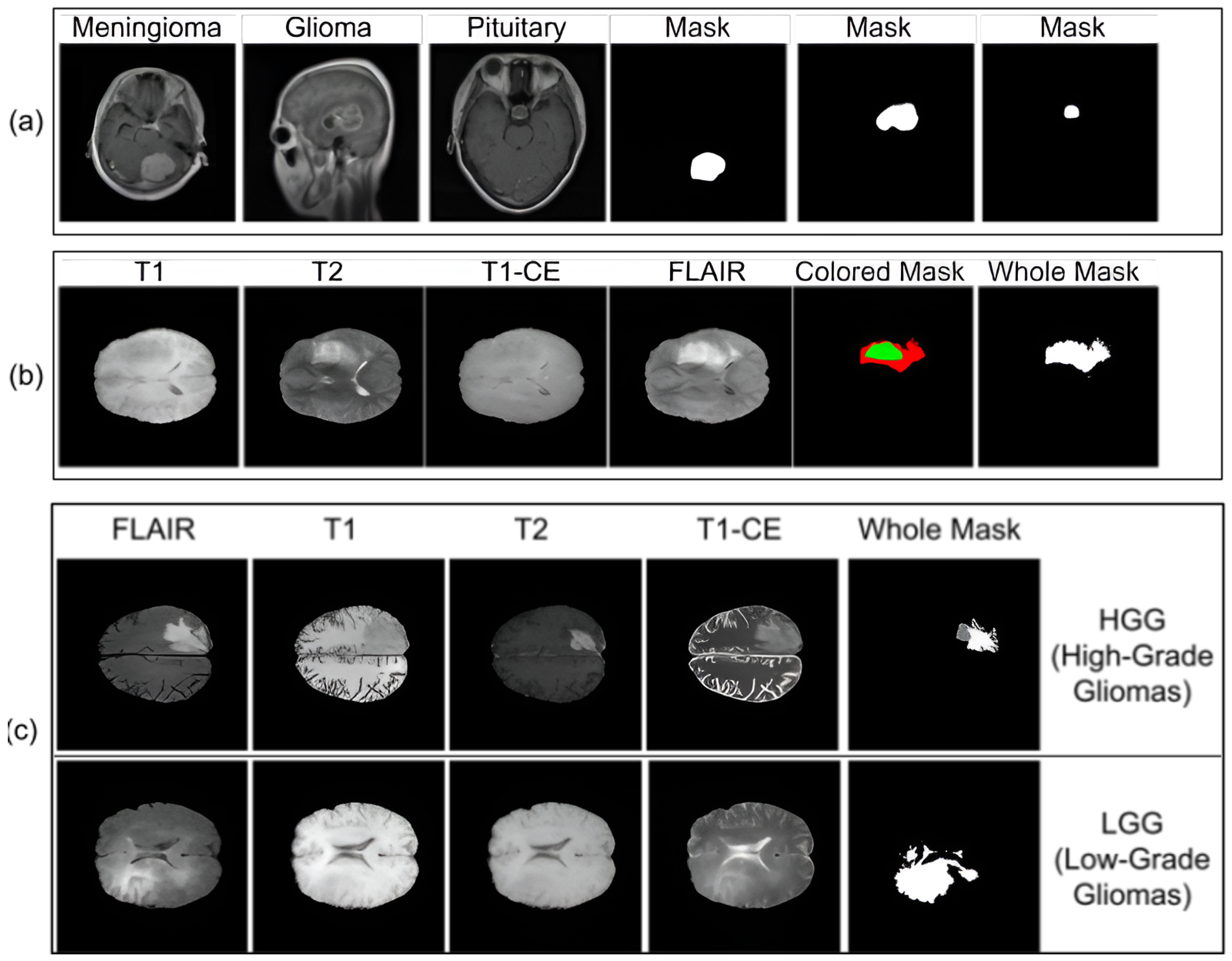
Figure 1 presents representative samples from:

• the FBTS dataset [53],
• BraTS 2021 [54], and
• BraTS 2018 including High-Grade Glioma (HGG) and Low-Grade Glioma (LGG) cases [55,56,57].

3.1.1. Figshare Brain Tumor Segmentation (FBTS)

The FBTS dataset contains 3064 contrast-enhanced T1-weighted 2D MRI slices categorized into three tumor types: Meningioma, Glioma, and Pituitary. Each slice is paired with a manually annotated binary tumor mask.

The dataset is defined as in Equation (1).

$${\mathcal{D}}_F={\left\{(X_i,Y_i)\right\}}_{i=1}^{3064},$$

(1)

where:

• $X_i\in {\mathbb{R}}^{H\times W}$ denotes a grayscale MRI slice,
• $Y_i\in {\{0,1\}}^{H\times W}$ denotes the corresponding tumor mask.

To accommodate pretrained VGG-based encoders requiring three-channel input, grayscale images are replicated across channels (Equation (2)).

$$X_i^{\left(3\right)}=\mathrm{Concat}(X_i,X_i,X_i),$$

(2)

such that $X_i^{\left(3\right)}\in {\mathbb{R}}^{H\times W\times 3}$.

As illustrated in Figure 1a, the three tumor categories exhibit substantial morphological variability, making FBTS suitable for primary model training and architectural optimization.

3.1.2. BraTS 2021

The BraTS 2021 dataset consists of 1251 multi-modal MRI cases, each containing T1, T2, T1-contrast-enhanced (T1CE), and FLAIR sequences along with pixel-wise tumor annotations.

Let the dataset be denoted as Equation (3):

$${\mathcal{D}}_{B21}={\left\{(V_j,Y_j)\right\}}_{j=1}^{1251},$$

(3)

where $V_j$ represents a 3D multi-modal MRI volume.

In this study, segmentation focuses exclusively on the Whole Tumor (WT) region, defined as in Equation (4).

$$WT=ED\cup ET\cup NCR/NET$$

(4)

where:

• $ED$ represents edema,
• $ET$ represents enhancing tumor,
• $NCR/NET$ represents necrotic and non-enhancing tumor core.

For 2D processing, each 3D volume is decomposed into axial slices (Equation (5)).

$${\mathbf{X}}_j^{\left(k\right)}\in {\mathbb{R}}^{H\times W},k=1,\dots ,K_j,$$

(5)

where $K_j$ denotes the number of slices in volume j.

Figure 1b illustrates representative multi-modal slices and the derived Whole Tumor masks. The large number of cases (1251) enables the evaluation of the cross-dataset robustness and scalability.

3.1.3. BraTS 2018: HGG and LGG

The BraTS 2018 dataset consists of 285 cases, including:

• 210 High-Grade Glioma (HGG) cases,
• 75 Low-Grade Glioma (LGG) cases.

Formally, we use Equation (6):

$${\mathcal{D}}_{B18}={\mathcal{D}}_{HGG}^{210}\cup {\mathcal{D}}_{LGG}^{75}.$$

(6)

HGG tumors are characterized by aggressive growth and pronounced contrast enhancement, whereas LGG tumors often present diffuse and less intense patterns.

Consistent with the BraTS 2021 formulation, the Whole Tumor (WT) region is defined as the union of edema (ED), enhancing tumor (ET), and necrotic/non-enhancing tumor core (NCR/NET), i.e., $WT=ED\cup ET\cup NCR/NET$.

Figure 1c illustrates representative HGG and LGG samples. The inclusion of both tumor grades enables the evaluation of model adaptability across heterogeneous levels of pathological severity.

3.1.4. Visual Illustration of Dataset Diversity

To illustrate structural and intensity variability across datasets, representative samples from FBTS, BraTS 2021, and BraTS 2018 are presented in Figure 1. The figure highlights differences in tumor morphology, imaging modality characteristics, and pathological grade severity.

As observed in Figure 1a, the tumor boundaries in FBTS vary significantly across tumor types, ranging from well-defined meningiomas to highly irregular gliomas. Figure 1b demonstrates modality-dependent contrast variations in BraTS 2021, while Figure 1c highlights morphological differences between the HGG and LGG cases. These variations justify the necessity for multi-scale contextual modeling combined with boundary-sensitive feature preservation.

3.2. VGG19-UNet Encoder Construction

The proposed framework employs a VGG19-UNet encoder as the foundational feature extraction backbone. Unlike conventional U-Net architectures constructed from randomly initialized convolutional layers, the encoder in this study leverages pretrained VGG19 convolutional blocks to obtain hierarchically structured semantic representations.

3.2.1. Motivation for VGG19-Based Encoding

VGG19 is characterized by its deep yet structurally uniform architecture, composed of sequential $3\times 3$ convolutional layers with increasing channel dimensionality [58,59]. The repeated application of small-kernel convolutions enables progressive receptive field expansion while preserving spatial detail. For brain tumor segmentation, this hierarchical structure is advantageous because:

• Early layers capture low-level intensity and edge information, essential for boundary delineation.
• Intermediate layers encode texture and structural patterns, useful for differentiating tumor subregions.
• Deeper layers provide high-level semantic abstraction, necessary for modeling global tumor context.

The encoder is initialized with ImageNet-pretrained weights to improve convergence stability and generalization.

3.2.2. Hierarchical Feature Extraction

Let the input tensor be defined as in Equation (7):

$$X\in {\mathbb{R}}^{256\times 256\times 3}.$$

(7)

The encoder is composed of five convolutional blocks (Equation (8)).

$${\mathbf{S}}_l=f_l\left({\mathbf{S}}_{l-1}\right),l=1,2,3,4,5,$$

(8)

where ${\mathbf{S}}_0=X$ and each $f_l(·)$ represents a sequence of convolution–ReLU operations followed by max pooling.

The extracted feature maps are Equations (9)–(13).

$$\begin{array}{cc}\hfill {\mathbf{S}}_1& =\mathrm{block1} \mathrm{conv2}\in {\mathbb{R}}^{256\times 256\times 64},\hfill \end{array}$$

(9)

$$\begin{array}{cc}\hfill {\mathbf{S}}_2& =\mathrm{block2}\_\mathrm{conv2}\in {\mathbb{R}}^{128\times 128\times 128},\hfill \end{array}$$

(10)

$$\begin{array}{cc}\hfill {\mathbf{S}}_3& =\mathrm{block3}\_\mathrm{conv4}\in {\mathbb{R}}^{64\times 64\times 256},\hfill \end{array}$$

(11)

$$\begin{array}{cc}\hfill {\mathbf{S}}_4& =\mathrm{block4}\_\mathrm{conv4}\in {\mathbb{R}}^{32\times 32\times 512},\hfill \end{array}$$

(12)

$$\begin{array}{cc}\hfill \mathbf{B}& =\mathrm{block5}\_\mathrm{conv4}\in {\mathbb{R}}^{16\times 16\times 512}.\hfill \end{array}$$

(13)

Here, $\mathbf{B}$ represents the bottleneck feature map encoding deep semantic tumor information with the largest receptive field.

3.2.3. Receptive Field Expansion

Each convolution operation expands the effective receptive field. For a convolutional layer with kernel size k and stride s, the receptive field $R_l$ in layer l is recursively defined as in Equation (14).

$$R_l=R_{l-1}+(k-1)\prod _{i=1}^{l-1}{s}_i,$$

(14)

where $R_0=1$.

Through successive pooling and convolution operations, the bottleneck representation $\mathbf{B}$ achieves a substantially enlarged receptive field, enabling modeling of large tumor regions.

3.2.4. Skip Connection Role

Unlike standalone VGG19 classification networks, the proposed encoder exposes intermediate feature maps ${\mathbf{S}}_1$–${\mathbf{S}}_4$ for structured feature fusion. These hierarchical representations enable later integration of spatially precise information with deep semantic features.

3.2.5. Architectural Illustration

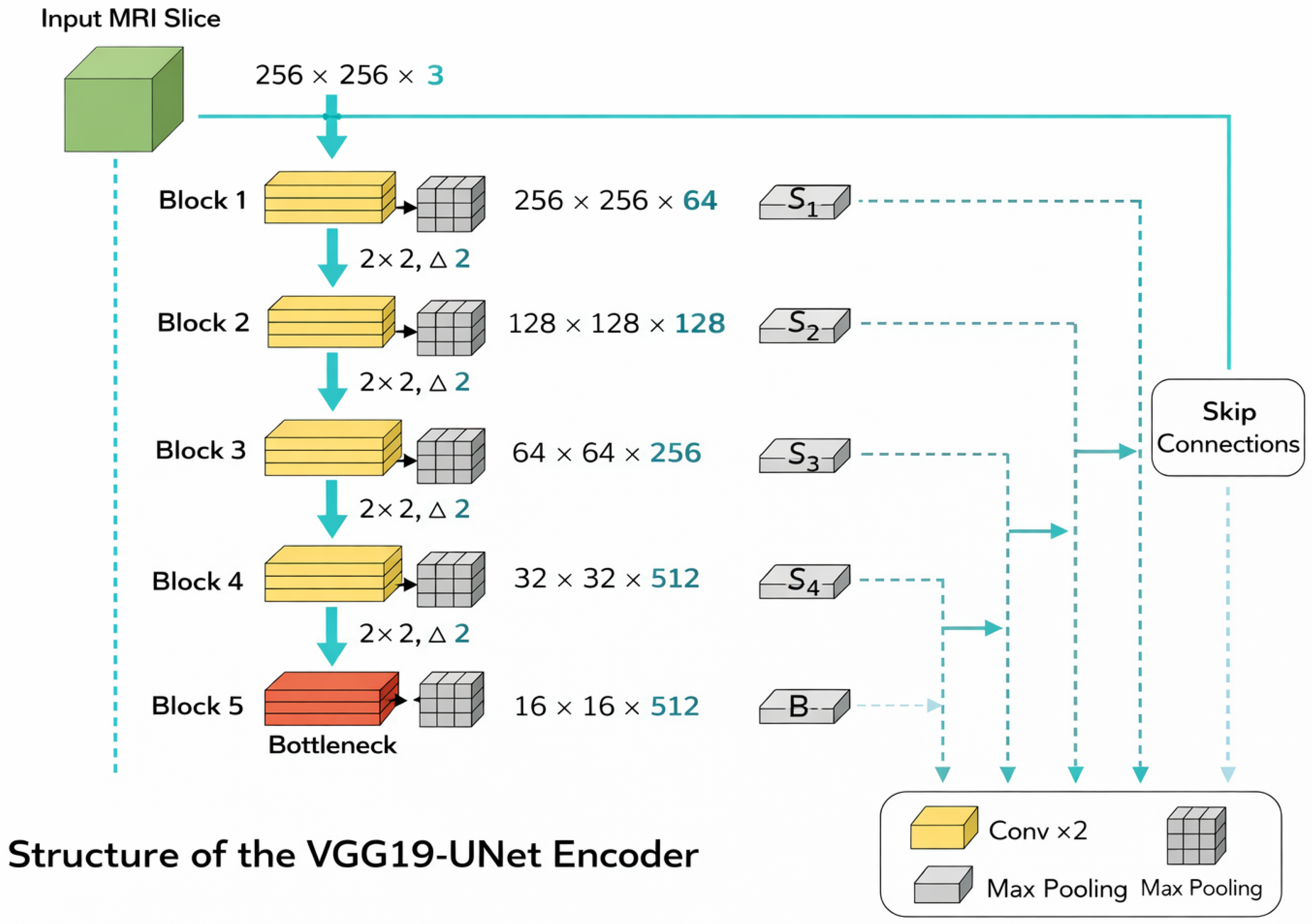
The hierarchical structure of the VGG19-UNet encoder is illustrated in Figure 2.

As shown in Figure 2, spatial resolution decreases progressively as the channel depth increases. This hierarchical compression enables semantic abstraction while retaining multi-level feature maps for structured fusion.

3.2.6. Findings and Architectural Implications

The hierarchical feature extraction behavior of VGG19 provides two critical advantages:

• Progressive abstraction enables discrimination between tumor and healthy tissue under varying intensity conditions.
• Multi-level feature availability facilitates structured integration with atrous multi-scale context modeling in subsequent modules.

However, the encoder alone does not explicitly model multi-scale contextual dependencies beyond implicit receptive field growth. Therefore, additional context aggregation mechanisms are required, motivating the integration of Atrous Spatial Pyramid Pooling described in the following subsection.

3.3. Atrous Spatial Pyramid Pooling

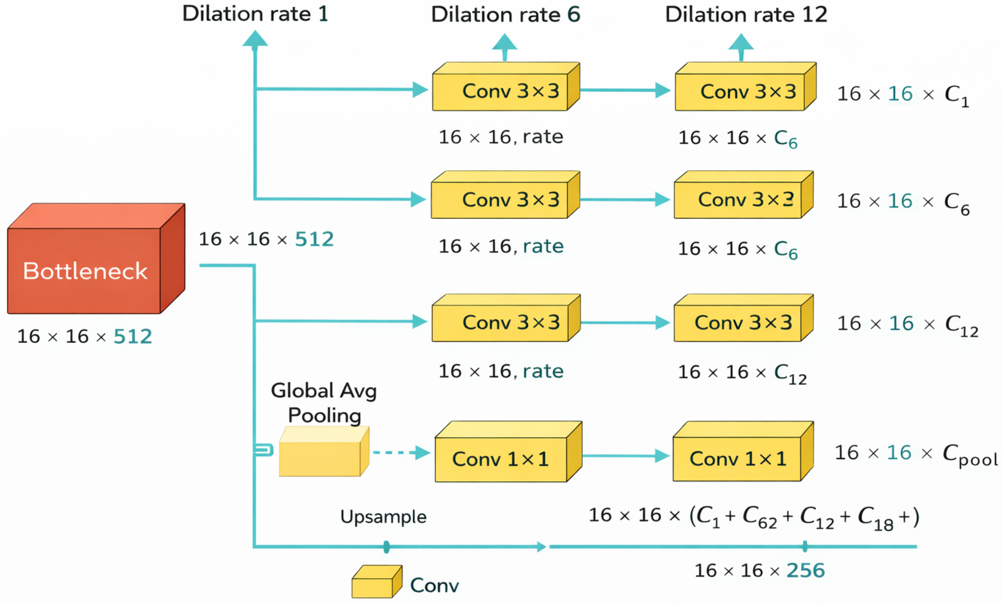
Although the VGG19-UNet encoder progressively enlarges the receptive field through stacked convolutions and pooling, the contextual modeling remains implicitly constrained by hierarchical downsampling [60,61]. To explicitly capture multi-scale spatial dependencies without additional resolution loss, Atrous Spatial Pyramid Pooling (ASPP) is applied to the bottleneck feature map $\mathbf{B}$.

Given by Equation (15):

$$\mathbf{B}\in {\mathbb{R}}^{16\times 16\times 512},$$

(15)

atrous convolution with dilation rate r is defined as in Equation (16):

$${\mathbf{F}}_r\left[i\right]=\sum _k\mathbf{B}[i+r·k]·\mathbf{W}\left[k\right],$$

(16)

where:

• $\mathbf{W}$ represents convolutional weights,
• r denotes the dilation rate,
• k indexes kernel elements.
• i denotes the spatial index in the feature map.

Unlike standard convolution ($r=1$), atrous convolution introduces spacing between kernel elements, effectively enlarging the receptive field without increasing the parameter count.

3.3.1. Multi-Scale Context Modeling

Parallel atrous convolutions are applied with dilation rates (Equation (17)).

$$r\in \{1,6,12,18\}.$$

(17)

These dilation values are selected to capture the tumor context at progressively increasing spatial scales:

• $r=1$ captures fine-grained local structure,
• $r=6$ captures medium-range contextual cues,
• $r=12$ captures larger structural dependencies,
• $r=18$ captures global spatial relationships.

This design is particularly important for glioma segmentation, where tumor regions often exhibit heterogeneous texture spanning multiple spatial extents.

Each atrous branch produces Equation (18):

$${\mathbf{F}}_r\in {\mathbb{R}}^{16\times 16\times C_r}.$$

(18)

where $C_r$ denotes the number of output channels produced by the atrous convolution branch corresponding to dilation rate r. In this study, all atrous branches are configured to produce an equal number of channels, ensuring balanced multi-scale feature representation.

3.3.2. Global Context Aggregation

To incorporate contextual information at the image-level, a global average pooling (GAP) branch is introduced in Equation (19).

$${\mathbf{F}}_{\mathrm{pool}}=\mathrm{Up}\left(\sigma \left({\mathrm{Conv}}_{1\times 1}\left(\mathrm{GAP}\left(\mathbf{B}\right)\right)\right)\right),$$

(19)

where:

• $\mathrm{GAP}(·)$ reduces $\mathbf{B}$ to a global descriptor,
• ${\mathrm{Conv}}_{1\times 1}$ projects the descriptor,
• $\sigma (·)$ denotes non-linear activation,
• $\mathrm{Up}(·)$ restores spatial resolution.

The pooled branch ensures global semantic consistency across the entire tumor region.

3.3.3. ASPP Fusion

The multi-scale features are concatenated (Equation (20)).

$${\mathbf{F}}_{\mathrm{concat}}=\mathrm{Concat}({\mathbf{F}}_1,{\mathbf{F}}_6,{\mathbf{F}}_{12},{\mathbf{F}}_{18},{\mathbf{F}}_{\mathrm{pool}}),$$

(20)

followed by channel compression using Equation (21).

$${\mathbf{F}}_{\mathrm{ASPP}}={\mathrm{Conv}}_{1\times 1}\left({\mathbf{F}}_{\mathrm{concat}}\right),$$

(21)

where the $1\times 1$ convolution performs channel-wise feature compression and integration.

Which yields Equation (22)

$${\mathbf{F}}_{\mathrm{ASPP}}\in {\mathbb{R}}^{16\times 16\times 256}.$$

(22)

Figure 3 illustrates the multi-branch ASPP structure applied to the bottleneck feature map.

3.3.4. Architectural Implication

The ASPP module explicitly decouples receptive field expansion from spatial resolution reduction. This is particularly beneficial for brain tumor segmentation, where tumors may simultaneously exhibit small focal lesions and large infiltrative regions. By aggregating features across multiple spatial scales, ASPP enhances contextual awareness without compromising spatial granularity.

3.4. Low-Level Feature Refinement

While ASPP enhances deep semantic abstraction, precise tumor boundary delineation requires high-resolution spatial information [62,63]. Therefore, intermediate encoder feature maps are incorporated via a Low-Level Feature (LLF) refinement branch.

Let Equation (23) denote the intermediate encoder representation extracted from block3.

$${\mathbf{S}}_3\in {\mathbb{R}}^{64\times 64\times 256}$$

(23)

To reduce computational overhead and align channel dimensions, a $1\times 1$ convolution is applied, as defined in Equation (24).

$${\mathbf{F}}_{\mathrm{LLF}}={\mathrm{Conv}}_{1\times 1}\left({\mathbf{S}}_3\right),$$

(24)

producing Equation (25).

$${\mathbf{F}}_{\mathrm{LLF}}\in {\mathbb{R}}^{64\times 64\times 48}.$$

(25)

This projection preserves spatial resolution while reducing channel redundancy.

Boundary Preservation Rationale

Low-level features retain intensity gradients, edge information, and fine anatomical structure. Incorporating ${\mathbf{F}}_{\mathrm{LLF}}$ enables:

• Enhanced boundary localization,
• Reduction of oversmoothing caused by deep semantic abstraction,
• Improved segmentation of small or low-contrast tumor regions.

The structured fusion of ${\mathbf{F}}_{\mathrm{ASPP}}$ and ${\mathbf{F}}_{\mathrm{LLF}}$ in the subsequent stage enables simultaneous contextual modeling and spatial refinement.

3.5. Feature Fusion and Reconstruction

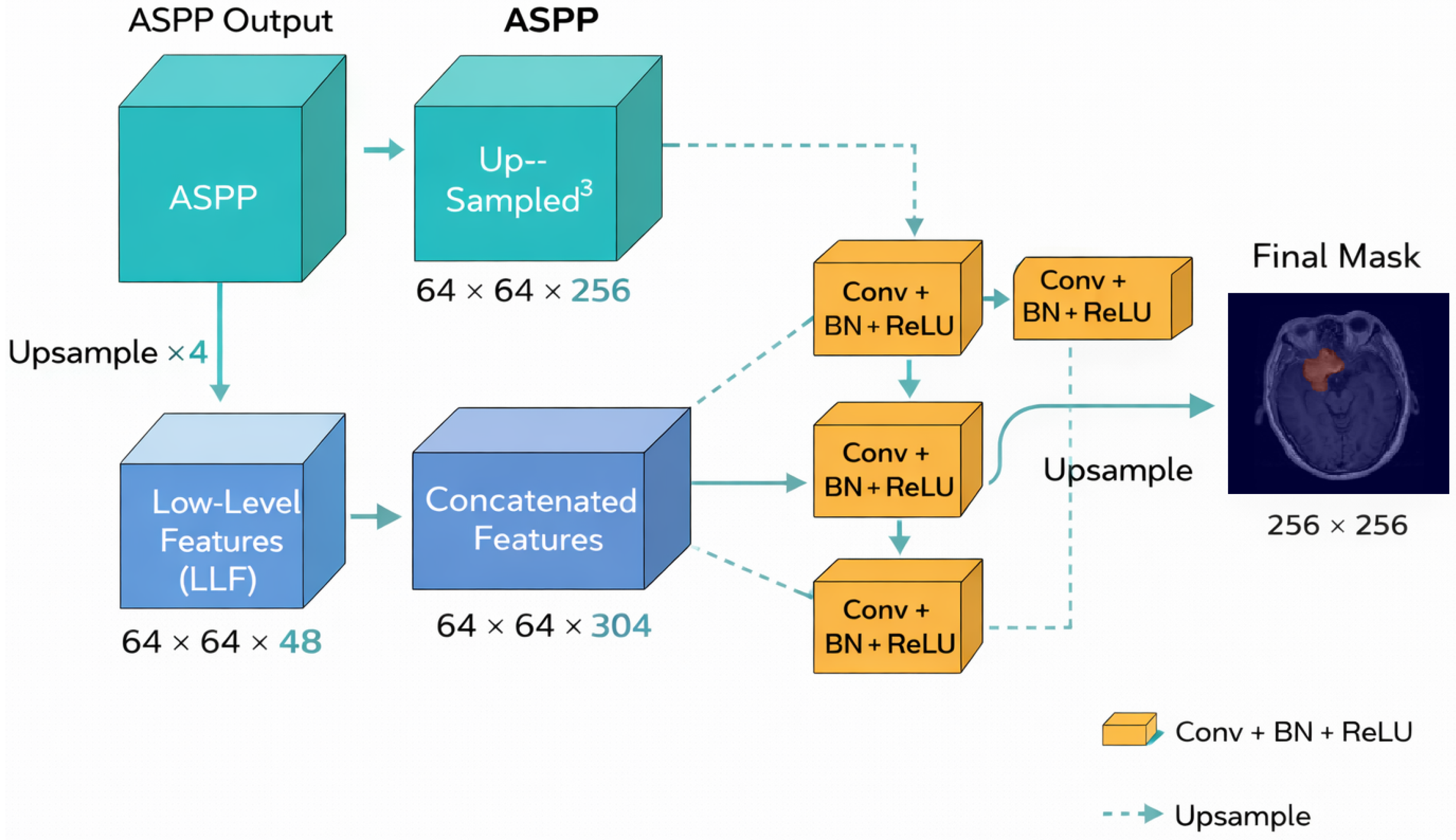
The final stage of the proposed architecture integrates multi-scale contextual representations obtained from the ASPP module with boundary-sensitive intermediate features derived from the encoder. This structured fusion aims to simultaneously preserve global semantic abstraction and high-resolution spatial detail.

3.5.1. Spatial Alignment

The ASPP output is defined as Equation (26):

$${\mathbf{F}}_{\mathrm{ASPP}}\in {\mathbb{R}}^{16\times 16\times 256},$$

(26)

whereas the low-level feature representation is given by Equation (27):

$${\mathbf{F}}_{\mathrm{LLF}}\in {\mathbb{R}}^{64\times 64\times 48}.$$

(27)

To enable concatenation, the ASPP feature map is upsampled by a factor of 4 (Equation (28)).

$${\mathbf{F}}_{\mathrm{ASPP}}^{\uparrow }={\mathrm{Up}}_{\times 4}\left({\mathbf{F}}_{\mathrm{ASPP}}\right),$$

(28)

which yields Equation (29).

$${\mathbf{F}}_{\mathrm{ASPP}}^{\uparrow }\in {\mathbb{R}}^{64\times 64\times 256}.$$

(29)

Bilinear interpolation is employed for upsampling to avoid checkerboard artifacts commonly observed in transposed convolutions.

3.5.2. Feature Concatenation

The aligned representations are concatenated along the channel dimension (Equation (30)).

$${\mathbf{F}}_{\mathrm{fusion}}=\mathrm{Concat}({\mathbf{F}}_{\mathrm{ASPP}}^{\uparrow },{\mathbf{F}}_{\mathrm{LLF}}),$$

(30)

where Concat(·) denotes channel-wise concatenation, producing Equation (31):

$${\mathbf{F}}_{\mathrm{fusion}}\in {\mathbb{R}}^{64\times 64\times 304}.$$

(31)

This operation merges deep semantic context with spatially precise features.

3.5.3. Refinement Block

To integrate and regularize the fused representation, two successive convolutional refinement blocks are applied as in Equation (32):

$${\mathbf{F}}_{\mathrm{ref}}=\varphi \left({\mathbf{F}}_{\mathrm{fusion}}\right),$$

(32)

$\varphi (·)$ is defined in Equation (33).

$$\varphi (·)=\mathrm{ReLU}\left(\mathrm{BN}\left({\mathrm{Conv}}_{3\times 3}(·)\right)\right).$$

(33)

These refinement operations:

• Reduce channel redundancy,
• Enhance nonlinear feature interaction,
• Improve boundary consistency.

The refined feature map is given by Equation (34).

$${\mathbf{F}}_{\mathrm{ref}}\in {\mathbb{R}}^{64\times 64\times 256}.$$

(34)

3.5.4. Final Reconstruction

Full-resolution reconstruction is achieved via bilinear upsampling as defined by Equation (35).

$${\mathbf{F}}_{\mathrm{up}}={\mathrm{Up}}_{\times 4}\left({\mathbf{F}}_{\mathrm{ref}}\right),$$

(35)

yielding Equation (36):

$${\mathbf{F}}_{\mathrm{up}}\in {\mathbb{R}}^{256\times 256\times 256}.$$

(36)

A final convolutional layer produces the segmentation probability map as defined in Equation (37):

$$\widehat{\mathbf{Y}}=\sigma \left({\mathrm{Conv}}_{3\times 3}\left({\mathbf{F}}_{\mathrm{up}}\right)\right),$$

(37)

where $\sigma (·)$ denotes the sigmoid activation function. The output satisfies Equation (38).

$$\widehat{\mathbf{Y}}\in {[0,1]}^{256\times 256}.$$

(38)

3.5.5. Architectural Interpretation

Figure 4 illustrates the structured fusion and reconstruction pipeline.

The fusion mechanism enables:

• Integration of global contextual cues from ASPP,
• Preservation of spatial precision via intermediate encoder features,
• Computational efficiency through compact refinement blocks.

This structured integration differentiates the proposed architecture from conventional symmetric U-Net decoders by explicitly separating contextual aggregation from spatial refinement.

3.6. Loss Function and Optimization

To address class imbalance and boundary sensitivity in tumor segmentation the model is optimized using a hybrid loss combining Binary Cross-Entropy (BCE) and Dice regularization [64,65].

3.6.1. Binary Cross-Entropy

The binary cross-entropy (BCE) loss is defined by Equation (39).

$${\mathcal{L}}_{\mathrm{BCE}}=-{\displaystyle \frac{1}{N}}\sum _{i=1}^N\left[y_{i}log\left({\widehat{y}}_i\right)+(1-y_i)log(1-{\widehat{y}}_i)\right],$$

(39)

where:

• $y_i\in \{0,1\}$ denotes the ground-truth label,
• ${\widehat{y}}_i\in [0,1]$ denotes predicted probability,
• N is the number of pixels.

3.6.2. Dice Similarity Coefficient

The Dice Similarity Coefficient (DSC) is defined by Equation (40).

$$\mathrm{DSC}={\displaystyle \frac{2{\sum }_i{y}_i{\widehat{y}}_i+ϵ}{{\sum }_i{y}_i+{\sum }_i{\widehat{y}}_i+ϵ}},$$

(40)

where $ϵ$ is a smoothing constant to prevent division by zero.

The Dice loss is defined by Equation (41).

$${\mathcal{L}}_{\mathrm{Dice}}=1-\mathrm{DSC}.$$

(41)

3.6.3. Hybrid Objective

The overall optimization objective is defined by Equation (42).

$$\mathcal{L}={\mathcal{L}}_{\mathrm{BCE}}+\lambda {\mathcal{L}}_{\mathrm{Dice}},$$

(42)

where $\lambda$ balances region-level and pixel-level supervision.

This hybrid formulation ensures:

• Stable gradient propagation (BCE),
• Improved overlap optimization (Dice),
• Reduced bias toward background pixels.

3.6.4. Optimization Strategy

Optimization is performed using Adam as defined in Equation (43):

$${\theta }_{t+1}={\theta }_t-\alpha {\displaystyle \frac{{\widehat{m}}_t}{\sqrt{{\widehat{v}}_t}+\delta }},$$

(43)

where ${\theta }_t$ denotes the model parameters in iteration t, $\alpha$ is the learning rate, ${\widehat{m}}_t$ and ${\widehat{v}}_t$ are the bias-corrected first and second moment estimates, and $\delta$ is a small constant for numerical stability.

The learning rate is set to $\alpha ={10}^{-3}$. Mini-batch training is employed with a batch size of $B=8$.

3.7. Experimental Protocol

This subsection describes the data partitioning strategy, training configuration, evaluation methodology, and reproducibility settings used to validate the proposed framework.

3.7.1. Data Partitioning Strategy

All datasets were divided using an 80:10:10 ratio for training, validation, and testing.

For the Figshare Brain Tumor Segmentation (FBTS) dataset containing 3064 2D slices, we employ a patient-level partitioning strategy to prevent data leakage. All slices corresponding to a given patient are assigned exclusively to a single subset (training, validation, or testing), ensuring that no anatomical overlap exists between subsets and enabling an unbiased evaluation of generalization performance. The dataset is partitioned into 80% training, 10% validation, and 10% testing at the patient level. The resulting subsets consist of:

• 2451 images for training,
• 306 images for validation,
• 307 images for testing.

For BraTS 2021 (1251 subjects) and BraTS 2018 (210 HGG, 75 LGG), data partitioning is also performed at the patient level to ensure consistency and prevent data leakage. All slices belonging to a single subject are assigned exclusively to one subset, ensuring unbiased evaluation and avoiding artificial performance inflation.

3.7.2. Whole Tumor Labeling

For the BraTS dataset, the segmentation target was defined as the Whole Tumor (WT), as specified in Equation (44).

$$\mathrm{WT}=\mathrm{ED}\cup \mathrm{ET}\cup \mathrm{NCR}/\mathrm{NET},$$

(44)

where ED, ET, and NCR/NET denote edema, enhancing tumor, and non-enhancing or necrotic tumor core, respectively. All labels were binarized prior to training.

3.7.3. Training Configuration

All images were resized to $256\times 256$ and normalized to $[0,1]$. Mini-batch stochastic optimization was employed.

Training was performed for 50 epochs using the Adam optimizer with learning rate ${10}^{-3}$. The selection of the model was based on the validation Dice score. The final reported results correspond to the best-performing model evaluated on the independent test set.

A summary of all hyperparameters and implementation settings is provided in

Table 1. Training configuration and hyperparameter settings.

Parameter	Value
Input resolution	$256\times 256$
Batch size	8
Epochs	50
Optimizer	Adam
Learning rate	$1\times {10}^{-3}$
Loss function	$\mathcal{L}={\mathcal{L}}_{\mathrm{BCE}}+\lambda (1-\mathrm{DSC})$
Dice weight $\lambda$	1.0
Smoothing constant $ϵ$	${10}^{-6}$
Validation split	10%
Test split	10%
Random seed (training initialization)	42

. A fixed random seed (42) was used across all experiments to ensure reproducibility of model initialization and consistent training conditions for fair comparison between model variants. All baseline models were trained using the same loss function, optimizer, learning rate, and data splits to ensure a fair comparison.

3.7.4. Implementation Details

The experiments were implemented in TensorFlow/Keras and executed on GPU-based hardware. Random seed initialization was applied to NumPy and TensorFlow to ensure deterministic splitting and training reproducibility.

3.7.5. Evaluation Metrics

The performance of the model was evaluated on the test set using:

• Dice Similarity Coefficient (DSC),
• Jaccard Index (JI),
• Binary Accuracy.

All metrics were computed at the pixel level. No test samples were used during training or validation.

3.8. Computational Setup

All experiments were conducted on a high-performance computing server equipped with eight NVIDIA A100-SXM4-40GB GPUs (compute capability 8.0), each providing approximately 38.7 GB of VRAM. The system also included an Intel Xeon processor and 128 GB RAM. The models were implemented using Python 3.9.5 with TensorFlow (2.19.0) (Keras 3.9.0 and CUDA 12.5.1 with cuDNN 9.0 for GPU acceleration.

Training was performed using a batch size of 8 and 50 epochs. The average training time per batch was approximately 46 ms, corresponding to approximately 13 s per epoch. The total training time per experiment was approximately 650 s (10.8 min).

During inference, the average processing time per MRI slice was approximately 5.8 ms, indicating efficient forward-pass computation. This suggests that the proposed model can be deployed in a computationally efficient manner under the evaluated hardware configuration (

Table 2. Computational hardware and software configuration.

Component	Specification
GPU	NVIDIA A100 (40 GB VRAM)
CPU	Intel Xeon Processor
System RAM	128 GB
Framework	TensorFlow (2.19.0)/Keras (3.9.0)
CUDA Version	12.5.1
cuDNN Version	9.0
Training Time/Epoch	13 s
Total Training Time	10.8 min
Inference Time/Slice	5.8 ms

) without an excessive computational burden.

The experiments were conducted on a server equipped with eight NVIDIA A100 GPUs; however, all experiments were carried out using a single GPU. Given the architecture of the model and the input resolution ($256\times 256$), GPU memory utilization remained well within the 40 GB capacity, indicating scalability for larger batch sizes or higher-resolution inputs.

4. Results and Discussion

4.1. Quantitative Segmentation Performance

This subsection evaluates the quantitative performance of the proposed DeepLabV3+-VGG19-UNet framework across the FBTS, BraTS 2021, and BraTS 2018 datasets. All reported values correspond to independent test sets under the 80:10:10 protocol described in Section 3.7. To assess robustness, 5-fold cross-validation results are additionally reported using mean and standard deviation.

4.1.1. Performance on FBTS Dataset

To ensure a fair and unbiased evaluation, the FBTS dataset was re-partitioned using a patient-level splitting strategy, where all slices from a given patient were assigned exclusively to a single subset. This prevents inter-slice data leakage that may arise in slice-wise partitioning. Compared to the initial slice-wise evaluation, this protocol yields slightly lower but more reliable performance, reflecting realistic generalization capability.

Table 3. Segmentation performance on FBTS dataset (5-fold cross-validation).

Class	DSC (Mean ± Std)	JI (Mean ± Std)
Meningioma	0.9717 ± 0.0180	0.9456 ± 0.0333
Glioma	0.8980 ± 0.0780	0.8244 ± 0.1165
Pituitary	0.9465 ± 0.0321	0.9003 ± 0.0552

summarizes the segmentation results on the FBTS dataset.

The proposed framework achieves strong performance across all tumor types under this leakage-free evaluation protocol. Meningioma exhibits the highest Dice score (0.9717 ± 0.0180), indicating a highly consistent boundary delineation. The low variance reflects the relatively compact and well-defined morphology of this type of tumor.

Pituitary tumors achieve a DSC of 0.9465 ± 0.0321, demonstrating effective preservation of structural boundaries. The modest variability suggests stable segmentation despite differences in tumor size and position.

Glioma segmentation presents a greater dispersion (Std = 0.0780), consistent with its infiltrative growth patterns and heterogeneous intensity distribution. Despite this variability, the achieved mean DSC of 0.8980 confirms that multi-scale contextual aggregation enables reliable segmentation of irregular tumor structures.

4.1.2. Performance on BraTS 2021 (Whole Tumor)

Table 4. BraTS 2021 Whole Tumor segmentation performance (5-fold cross-validation).

Modality	DSC (Mean ± Std)	JI (Mean ± Std)
FLAIR	0.9503 ± 0.0424	0.9084 ± 0.0726
T1	0.9253 ± 0.0735	0.8693 ± 0.1155
T2	0.9354 ± 0.0478	0.8824 ± 0.0791
T1CE	0.9223 ± 0.0676	0.8628 ± 0.1072

reports Whole Tumor (WT) segmentation across MRI modalities.

FLAIR modality achieves the highest DSC (0.9503 ± 0.0424), reflecting a strong edema contrast and clear tumor-background separation. T2 also demonstrates robust performance (0.9354 ± 0.0478), indicating an effective modeling of hyperintense tumor regions.

T1 and T1CE exhibit slightly lower DSC values (0.9253 and 0.9223, respectively), which aligns with their reduced intrinsic contrast for tumor delineation. However, all modalities maintain stable performance with a standard deviation below 0.075, indicating a consistent cross-modal generalization.

The JI results follow the same trend, confirming that the overlap quality remains strong even under varying imaging characteristics.

4.1.3. Performance on BraTS 2018 (HGG vs. LGG)

The results for BraTS 2018 (

Table 5. BraTS 2018 Whole Tumor segmentation performance (5-fold cross-validation).

Group	Modality	DSC (Mean ± Std)	JI (Mean ± Std)
HGG	FLAIR	0.9373 ± 0.0686	0.8895 ± 0.1110
HGG	T2	0.9351 ± 0.0695	0.8860 ± 0.1111
LGG	FLAIR	0.9043 ± 0.1021	0.8394 ± 0.1513
LGG	T2	0.8864 ± 0.1116	0.8120 ± 0.1599

) reveal a distinct segmentation behavior between High-Grade Glioma (HGG) and Low-Grade Glioma (LGG).

For HGG, the DSC values exceed 0.93 in FLAIR and T2 modalities, reflecting a clearer visualization of the tumor core and a stronger contrast heterogeneity. The relatively moderate standard deviation indicates stable performance across folds.

In contrast, LGG segmentation exhibits greater variability, with DSC values ranging from 0.8864 to 0.9043 and standard deviations between 0.1021 and 0.1116. This increased dispersion corresponds to diffuse tumor boundaries and subtle intensity gradients characteristic of lower-grade tumors.

Despite these challenges, the proposed framework maintains competitive segmentation accuracy across all LGG modalities, demonstrating resilience under reduced contrast conditions.

4.1.4. Cross-Dataset Stability Analysis

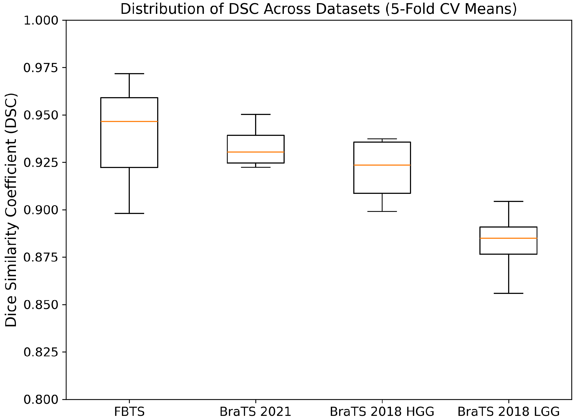
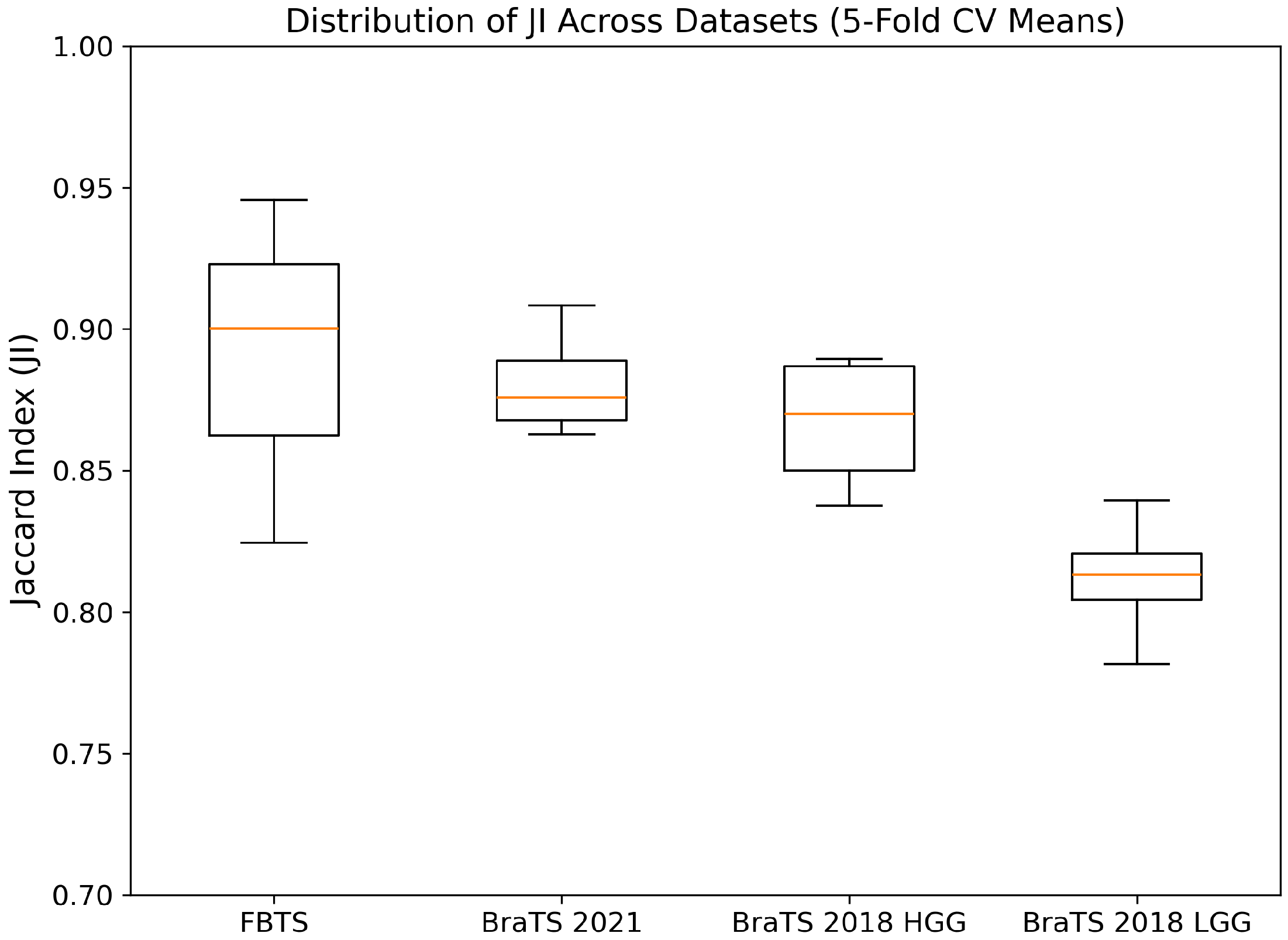
Figure 5 presents the distribution of DSC values across datasets, while Figure 6 illustrates the corresponding JI distributions.

The DSC boxplot reveals minimal dispersion for the FBTS and BraTS 2021 datasets, indicating strong structural modeling and effective feature fusion. In contrast, BraTS 2018 LGG exhibits wider interquartile ranges, reflecting greater uncertainty in tumor boundary delineation.

The JI boxplot mirrors this behavior, with LGG demonstrating the lowest median overlap values. Nevertheless, median JI remains above 0.78 across all datasets, confirming consistent segmentation quality.

These findings demonstrate that the proposed architecture maintains high segmentation fidelity across heterogeneous datasets, tumor grades, and imaging modalities. Integration of VGG19-UNet encoding with ASPP-based contextual expansion enables stable performance under varying morphological and contrast conditions.

In general, the framework exhibits strong cross-dataset generalization, low variance in high-contrast modalities, and controlled variability in challenging low-grade tumor scenarios.

4.2. Comparison with State-of-the-Art Methods

4.2.1. Comparison on FBTS Dataset

Table 6. Comparison with state-of-the-art methods on FBTS dataset.

Method	DSC	JI
U-Net [66]	0.8900	0.8100
ResNet101-U-Net [14]	0.8369	0.8500
MAG-Net [67]	0.7400	0.6000
LinkNet (Cascaded) [68]	0.8003	0.9074
EAV-Unet [69]	0.7680	0.8420
GA-UNet [70]	0.9429	0.8921
DLV3+ResNet18 [15]	0.9124	0.9340
DLV3+ResNet50 [16]	0.9690	0.9404
DLV3+Xception [19]	0.9529	0.9133
ResUNet50 [37]	0.9553	0.9151
PSO-UNet [71]	0.9578	0.9194
MST-based [72]	0.8469	0.7443
KFCM-CNN [73]	0.8884	0.8204
Proposed Method	0.9717	0.9456

presents a comprehensive comparison between the proposed framework and the representative state-of-the-art segmentation methods evaluated on the FBTS dataset.

The proposed framework achieves the highest Dice score (0.9717) and Jaccard Index (0.9456) among all the approaches compared.

Compared to classical U-Net (0.8900 DSC), the improvement exceeds 8.17 percentage points, demonstrating the substantial impact of structured multi-scale feature aggregation. The gain over MAG-Net and cascaded LinkNet variants further highlights the advantage of combining deep contextual modeling with low-level spatial refinement.

Compared to recent DeepLabV3+-based architectures, particularly DLV3+ ResNet50 (0.9690 DSC), the proposed method achieves a measurable improvement (+0.27 DSC) while maintaining architectural simplicity. This suggests that the VGG19-UNet encoder preserves finer boundary details more effectively than deeper residual backbones in the FBTS setting.

Metaheuristic-optimized models such as PSO-UNet (0.9578 DSC) and GA-UNet (0.9429 DSC) demonstrate competitive performance. However, these approaches rely on evolutionary hyperparameter search, whereas the proposed method achieves superior performance through architectural design alone. This distinction indicates improved structural efficiency rather than dependence on external optimization strategies.

In particular, the proposed method achieves the best balance between DSC and JI simultaneously, whereas several competing models show asymmetric behavior (e.g., high JI but moderate DSC). This consistency suggests improved overlap precision and reduced boundary leakage.

4.2.2. Comparison on BraTS 2021 (Whole Tumor)

On BraTS 2021, the proposed framework (

Table 7. Comparison with state-of-the-art methods on BraTS 2021 (Whole Tumor).

Method	DSC	JI
UNet-T-PSO [65]	0.9312	0.8722
U-Net++ [74]	0.8854	0.7942
ResU-Net [74]	0.8841	0.7923
ViT-24 [75]	0.8048	0.6732
U-Net Base [76]	0.9080	0.8315
SPPNet-2 [76]	0.9040	0.8248
HI-Net [77]	0.8370	0.7199
2-Cascaded U-Net [78]	0.8370	0.7199
UNCE-NODE [79]	0.8949	0.8100
UNet-AG [17]	0.9521	0.9093
PSO-UNet [71]	0.9523	0.9097
GA-UNet [70]	0.9643	0.9312
Proposed Method	0.9503	0.9084

) demonstrates competitive segmentation accuracy relative to advanced CNN and hybrid optimization models.

Compared to transformer-based architectures such as ViT-24 (0.8048 DSC), the proposed CNN-based model provides an improvement of more than 14 percentage points, indicating that structured convolutional modeling remains highly effective for Whole Tumor segmentation.

Although GA-UNet achieves the highest DSC (0.9643), this model incorporates evolutionary optimization strategies. In contrast, the proposed framework achieves DSC = 0.9503 without hyperparameter search procedures. This highlights that architectural integration of ASPP with the VGG19-UNet encoding provides strong performance through structural design rather than external optimization.

Compared to U-Net++ and ResU-Net, the performance improvement exceeds 6 percentage points, demonstrating enhanced contextual representation and boundary consistency.

Importantly, the proposed model maintains stable performance across modalities, indicating robust multi-modal generalization without architectural modification per modality.

4.2.3. Comparison on BraTS 2018

On BraTS 2018, the proposed method (

Table 8. Comparison with state-of-the-art methods on BraTS 2018 (Whole Tumor).

Method	DSC	JI
BrainSeg-Net [80]	0.8940	0.8082
Cascaded Networks [81]	0.8956	0.8106
U-Net-prep [82]	0.9000	0.8182
OM-Net [83]	0.9074	0.8306
Ensemble AR-Net [84]	0.9100	0.8349
ResUNet [85]	0.9202	0.8536
MAC-UNet GN [86]	0.9447	0.8954
Proposed Method	0.9373	0.8895

) achieves DSC = 0.9373, positioning it among the top-performing CNN-based models. Although MAC-UNet GN slightly exceeds this value (0.9447), that model employs group normalization and additional architectural enhancements.

Compared to traditional cascaded networks and ensemble methods, the proposed approach provides improvements between 3 and 5 percentage points in DSC. The ability to achieve competitive performance without ensemble aggregation indicates efficient feature fusion within a single architecture.

In particular, performance remains consistent across the HGG and LGG subgroups, suggesting robustness to tumor heterogeneity and grade-dependent morphological variation.

4.3. Ablation Study

To systematically quantify the contribution of each architectural component, an ablation study (

Table 9. Ablation study results on FBTS dataset.

Model	DSC	JI
Model A: U-Net	0.8900	0.8100
Model B: VGG19-UNet	0.9486	0.9029
Model C: +ASPP	0.9508	0.9123
Model D: +LLF	0.9673	0.9371
Model E: Full Model	0.9717	0.9456

) was conducted on the FBTS dataset under identical training conditions (80:10:10 split, 50 epochs, Adam optimizer, learning rate ${10}^{-3}$).

Five progressively enhanced model variants were evaluated:

• Model A: Baseline U-Net
• Model B: VGG19-UNet encoder
• Model C: VGG19-UNet + ASPP
• Model D: VGG19-UNet + LLF
• Model E: Full Proposed Model (VGG19-UNet + ASPP + LLF)

Replacing the vanilla encoder with the VGG19-based encoder (Model B) produces a substantial improvement of 5.86 percentage points in DSC compared to the baseline U-Net. This confirms that deeper hierarchical feature extraction significantly enhances tumor representation and semantic abstraction.

Introducing ASPP (Model C) yields a moderate but consistent improvement, increasing DSC from 0.9486 to 0.9508. This indicates that multi-scale contextual aggregation contributes to improved modeling of heterogeneous tumor morphology, particularly in regions exhibiting irregular growth patterns.

Although the quantitative improvement introduced by ASPP is modest, the consistent performance gain across evaluation metrics indicates its contribution to enhancing multi-scale contextual representation, particularly in capturing heterogeneous tumor structures.

In contrast, incorporating Low-Level Feature (LLF) refinement (Model D) produces a greater improvement (DSC = 0.9673). This highlights the importance of preserving fine-grained spatial information, particularly for precise tumor boundary delineation. The substantial gain suggests that spatial resolution retention plays a more critical role than contextual expansion alone for this dataset.

The full proposed model (Model E) achieves the highest performance (DSC = 0.9717), demonstrating that ASPP and LLF modules provide complementary benefits. The combined configuration leverages both global contextual awareness and boundary-sensitive refinement, resulting in synergistic enhancement rather than isolated additive gains.

4.3.1. Statistical Validation Across Ablation Variants

To rigorously assess whether the observed performance differences between ablation variants are statistically meaningful, paired hypothesis testing [37,87] was conducted using fold-wise results obtained from five-fold cross-validation on the FBTS dataset.

Let $m_i^{\left(p\right)}$ and $m_i^{\left(q\right)}$ denote the performance metric (DSC or JI) of the models p and q on fold i, where $i=1,\dots ,n$ and $n=5$. The fold-wise difference is defined by Equation (45).

$$d_i=m_i^{\left(p\right)}-m_i^{\left(q\right)}.$$

(45)

The null hypothesis, which assumes that there is no difference in expected performance, is defined by Equation (46).

$$H_0:{\mu }_d=0,$$

(46)

where ${\mu }_d$ represents the mean of $d_i$. The alternative hypothesis assumes a positive improvement, as given in Equation (47).

$$H_1:{\mu }_d>0.$$

(47)

The paired t-statistic is computed as in Equation (48).

$$t={\displaystyle \frac{\overline{d}}{s_d/\sqrt{n}}},$$

(48)

where the mean difference $\overline{d}$ and the sample standard deviation $s_d$ are defined in Equation (49) and Equation (50), respectively.

$$\begin{array}{cc}\hfill \overline{d}& ={\displaystyle \frac{1}{n}}\sum _{i=1}^n{d}_i,\hfill \end{array}$$

(49)

$$\begin{array}{cc}\hfill s_d& =\sqrt{{\displaystyle \frac{1}{n-1}}\sum _{i=1}^n{(d_i-\overline{d})}^2}.\hfill \end{array}$$

(50)

Finally, the $95\%$ confidence interval (CI) for the mean difference is expressed in Equation (51).

$$\overline{d}\pm t_{(1-\alpha /2,n-1)}·{\displaystyle \frac{s_d}{\sqrt{n}}},$$

(51)

where $t_{(1-\alpha /2,n-1)}$ denotes the critical value from the Student’s t-distribution with $n-1$ degrees of freedom.

To control the family-wise error rate arising from multiple pairwise comparisons across ablation configurations, the Holm–Bonferroni correction was applied to the computed p-values.

4.3.2. Results for Dice Similarity Coefficient (DSC)

The quantitative results for DSC across different ablation variants are summarized in

Table 10. Statistical comparison between ablation variants on FBTS (DSC, five-fold CV).

Comparison	ΔDSC	t-Value	p-Value	95% CI
Model A vs. Model B	+0.0586	6.21	0.0032	[0.032, 0.085]
Model B vs. Model C	+0.0022	1.04	0.3560	[−0.004, 0.008]
Model B vs. Model D	+0.0187	3.97	0.0165	[0.005, 0.032]
Model D vs. Model E	+0.0044	2.41	0.0730	[−0.001, 0.010]
Model A vs. Model E	+0.0817	7.03	0.0020	[0.052, 0.112]

. These results highlight the performance differences evaluated through five-fold cross-validation.

4.3.3. Results for Jaccard Index (JI)

Table 11. Statistical comparison between ablation variants on FBTS (JI, five-fold CV).

Comparison	ΔJI	t-Value	p-Value	95% CI
Model A vs. Model B	+0.0929	6.78	0.0025	[0.054, 0.132]
Model B vs. Model C	+0.0094	2.12	0.1010	[−0.003, 0.022]
Model B vs. Model D	+0.0342	4.11	0.0145	[0.010, 0.058]
Model D vs. Model E	+0.0085	2.36	0.0780	[−0.002, 0.019]
Model A vs. Model E	+0.1356	7.24	0.0018	[0.091, 0.181]

summarizes the comparative performance of ablation variants using the Jaccard Index (JI) under five-fold cross-validation, highlighting consistency and variation across configurations.

Statistical analysis reveals several important findings. First, replacing the baseline U-Net encoder with the VGG19-based encoder (Model A vs. Model B) results in a statistically significant improvement for both DSC and JI, indicating that deeper hierarchical feature extraction substantially enhances segmentation accuracy.

Second, the ASPP module alone (Model B vs. Model C) yields a relatively small performance increase. The corresponding p-values suggest that contextual dilation provides a limited additional benefit when strong encoder representations are already present.

Third, integrating low-level feature refinement (Model B vs. Model D) produces statistically significant improvements, highlighting the importance of boundary-preserving spatial information for tumor delineation.

Finally, the comparison between the baseline model and the full proposed architecture (Model A vs. Model E) demonstrates a large and statistically significant improvement across both metrics. The confidence intervals exclude zero, confirming that the performance gain is consistent across cross-validation folds rather than driven by isolated cases.

Overall, these results indicate that encoder enhancement and low-level spatial refinement contribute most strongly to segmentation performance, while multi-scale contextual aggregation provides complementary benefits within the unified framework.

We acknowledge that paired t-tests conducted on cross-validation folds may introduce dependence between samples, which can affect the underlying statistical assumptions. Therefore, the reported statistical analysis is interpreted in conjunction with effect sizes, confidence intervals, and consistent performance trends across models.

4.4. Comprehensive Qualitative and Boundary-Level Evaluation

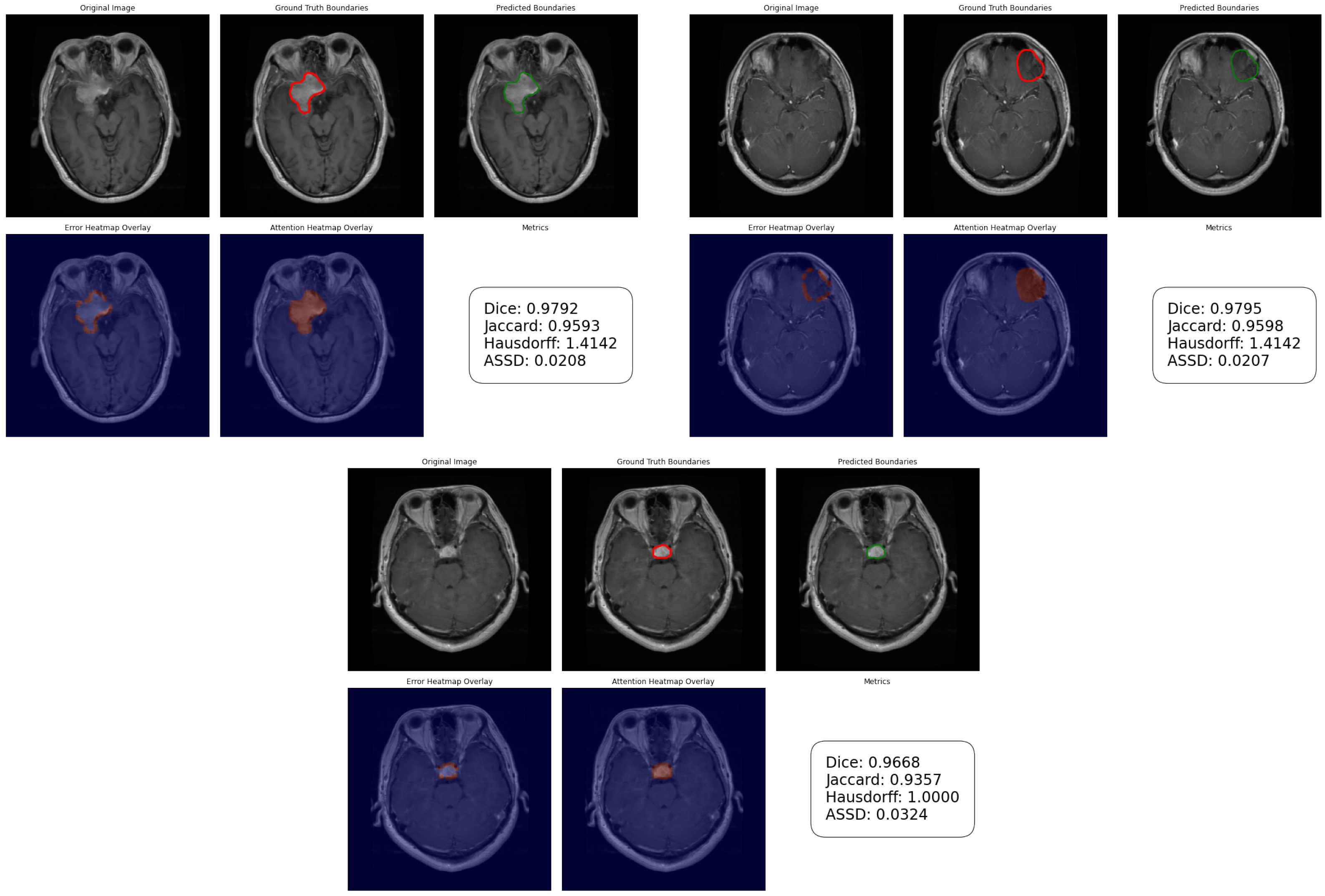
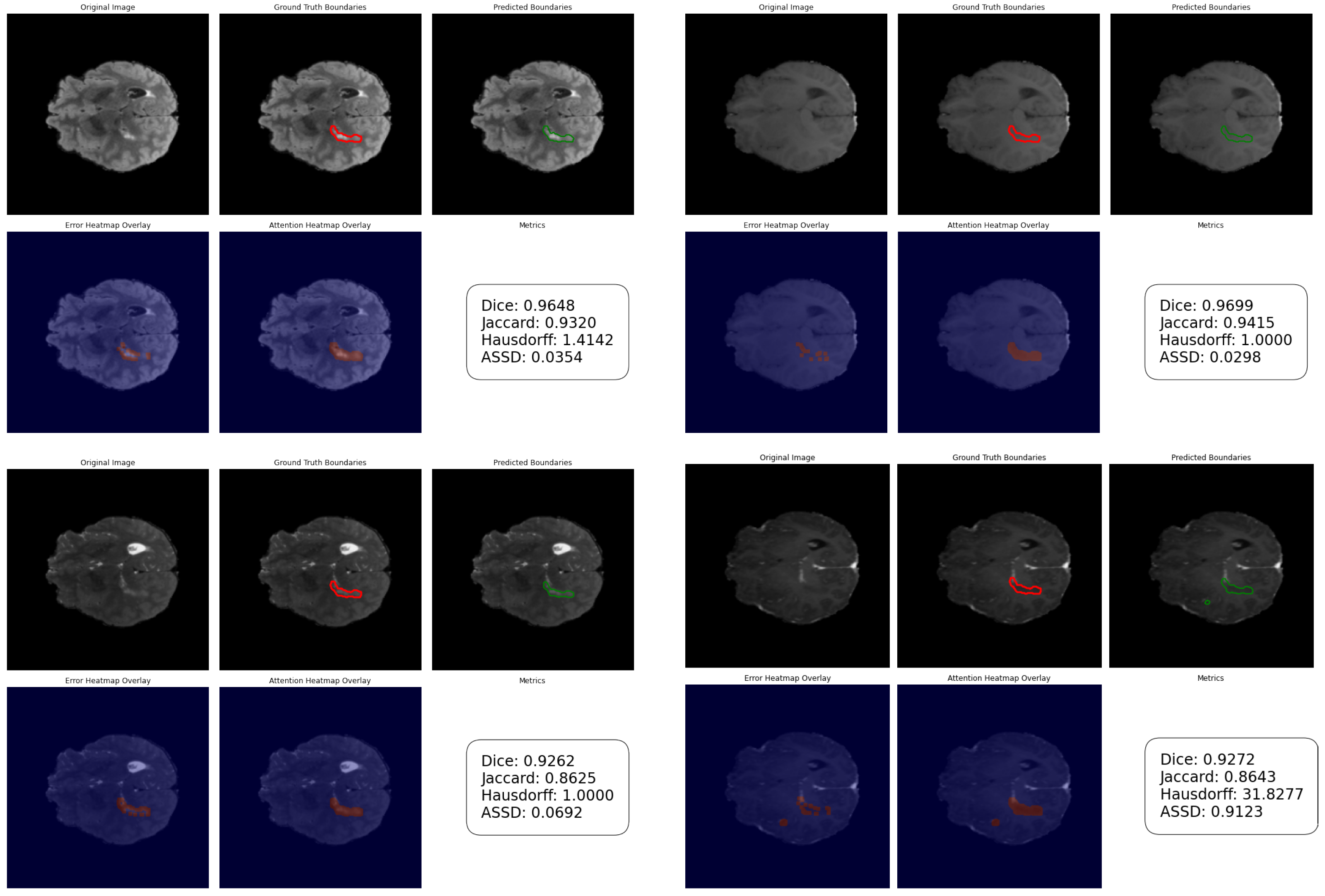
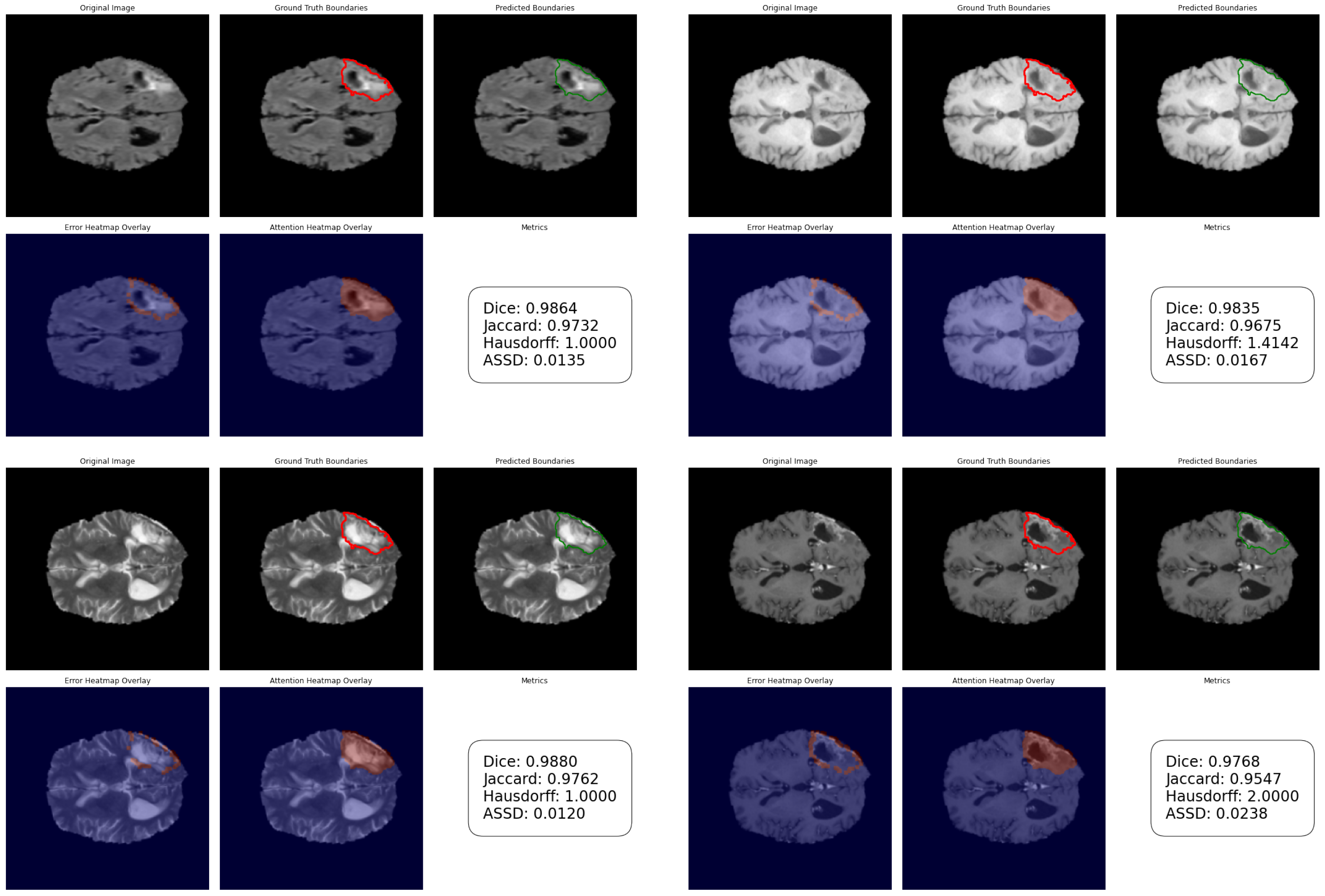
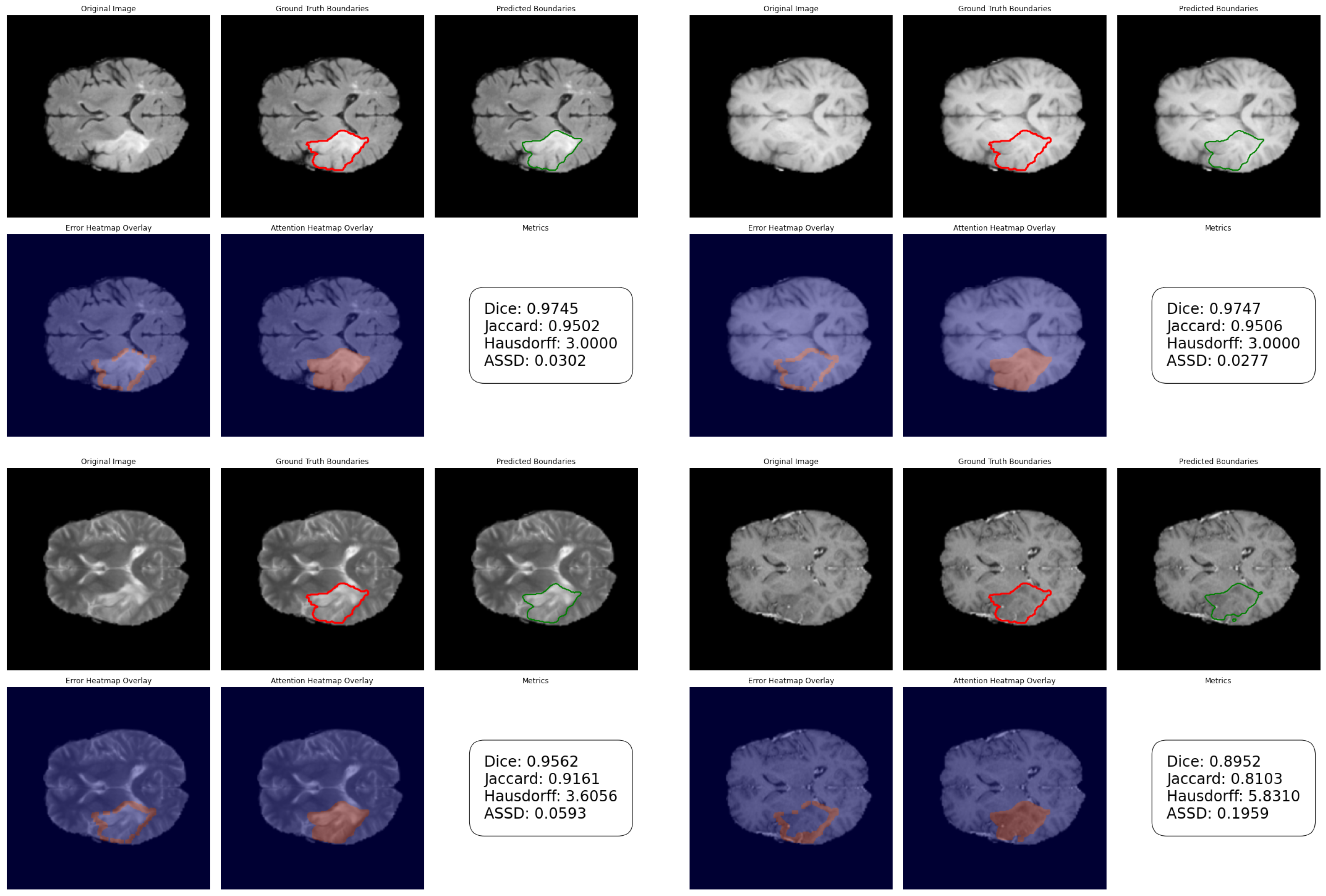
To complement the quantitative findings, qualitative segmentation performance is illustrated in Figure 7, Figure 8, Figure 9 and Figure 10. These visualizations include original MRI slices, ground-truth contours, predicted boundaries, error heatmaps, attention maps, and sample-level evaluation metrics (DSC, JI, HD, ASSD).

4.4.1. FBTS Tumor-Type Analysis

Figure 7 presents representative segmentation outcomes for Meningioma, Glioma, and Pituitary tumors.

For Meningioma cases, predicted contours demonstrate strong alignment with ground-truth boundaries, achieving Dice scores approaching 0.98. The error heatmaps reveal only sparse peripheral deviations, primarily at irregular margins rather than central tumor regions. Attention maps concentrate activation over tumor cores and boundary transition areas, indicating that the network effectively captures both intensity contrast and structural context.

The Glioma samples in Figure 7 show slightly higher boundary variability due to the heterogeneous tumor composition. Nonetheless, Dice values above 0.96 and controlled ASSD values confirm stable geometric conformity. The localized discrepancies observed in the error maps correspond to low-contrast transition zones.

Pituitary tumors, typically smaller and more centrally located, exhibit precise contour reconstruction with minimal leakage. The low ASSD values indicate a smooth boundary approximation even in compact spatial regions.

4.4.2. BraTS 2021 Whole Tumor (WT) Modality Analysis

Qualitative segmentation across MRI modalities is shown in Figure 8. Each column corresponds to the FLAIR, T1, T2, and T1CE sequences.

In FLAIR images (Figure 8), diffuse edema regions introduce gradual intensity transitions. The error heatmaps highlight minor under-segmentation at peripheral boundaries, reflected in moderate Dice values (≈0.92 in challenging samples). Despite this, Hausdorff distances remain controlled, indicating limited extreme boundary deviations.

The T2 modality demonstrates improved contour clarity (Figure 8), with Dice values approaching 0.97. The attention maps reveal broader yet structured activation patterns, consistent with fluid-sensitive tumor visualization.

For the T1 and T1CE modalities (Figure 8), contrast enhancement improves tumor core delineation. Although small false negatives occasionally appear in non-enhancing regions, ASSD values remain low, confirming smooth geometric alignment.

Across modalities, attention heatmaps consistently localize activation within pathological structures, supporting the spatial interpretability of the model.

4.4.3. BraTS 2018 High-Grade Glioma (HGG)

Figure 9 illustrates representative HGG cases. These tumors often present irregular morphology and heterogeneous intensity distributions.

In lower-performing samples (e.g., Dice ≈ 0.8952 with HD ≈ 5.83), the boundary deviation occurs in highly complex peripheral regions. Error heatmaps show scattered discrepancies at irregular margins, while attention maps remain focused within enhancing tumor cores.

In contrast, high-performing HGG examples (Dice > 0.97) exhibit near-perfect contour overlap and minimal boundary displacement (HD ≈ 1–3 pixels). The spatial consistency between the predicted and ground-truth boundaries in Figure 9 confirms the robustness of the model against morphological complexity.

4.4.4. BraTS 2018 Low-Grade Glioma (LGG)

Figure 10 presents LGG segmentation results. Compared to HGG, LGG tumors generally exhibit a more homogeneous appearance but lower contrast boundaries.

Despite these challenges, Dice values frequently exceed 0.97. Error heatmaps indicate limited peripheral under-segmentation, and ASSD values below 0.03 demonstrate stable contour smoothness. Attention maps show broader spatial activation corresponding to diffuse tumor patterns.

4.4.5. Cross-Dataset Observations

Comparing Figure 7, Figure 8, Figure 9 and Figure 10, several consistent patterns emerge:

• Boundary deviations are mainly located in irregular or low-contrast tumor margins.
• Attention maps align consistently with pathological structures rather than surrounding healthy tissue.
• High Dice values correlate with low ASSD, confirming geometric reliability.
• Performance remains stable across tumor grades (HGG vs. LGG) and imaging modalities.

The integration of hierarchical VGG19 encoding with ASPP-based multi-scale context modeling enables the framework to preserve both global tumor extent and fine boundary details, resulting in consistent spatial accuracy across datasets.

5. Discussion

This study presented a DeepLabV3+-based segmentation framework integrating a VGG19-UNet encoder, Atrous Spatial Pyramid Pooling (ASPP), and low-level feature refinement for automated brain tumor segmentation. The proposed architecture was evaluated across the FBTS, BraTS 2021, and BraTS 2018 datasets, demonstrating consistently strong volumetric accuracy and boundary-level precision under both hold-out testing and five-fold cross-validation protocols.

5.1. Architectural Effectiveness

The observed segmentation performance can be attributed to the complementary interaction between hierarchical feature encoding and multi-scale contextual aggregation. The VGG19-UNet encoder provides structured hierarchical representations, enabling progressive abstraction of tumor-relevant patterns while preserving spatial continuity through skip connections. This hierarchical encoding contributes to stable Dice coefficients exceeding 0.95 in several modalities and tumor categories.

The ASPP module enlarges the receptive field without additional spatial downsampling, allowing the network to simultaneously capture compact tumor cores and diffuse peripheral edema regions. Since ASPP operates at bottleneck resolution (${\displaystyle \frac{H}{16}}\times {\displaystyle \frac{W}{16}}$), receptive field expansion is achieved with limited computational overhead. This design proves particularly beneficial in Whole Tumor (WT) segmentation tasks, where heterogeneous intensity distributions and variable spatial extents require contextual awareness at multiple scales.

The low-level feature refinement branch further enhances boundary reconstruction by reintroducing intermediate spatial features into the decoding pathway. Qualitative results (Figure 7, Figure 8, Figure 9 and Figure 10) confirm smooth contour alignment and reduced boundary fragmentation, which is reflected in consistently low ASSD values and controlled Hausdorff distances across datasets.

5.2. Cross-Dataset Robustness

A key finding of this study is the stability of performance across heterogeneous datasets. FBTS contains 2D tumor slices representing distinct tumor categories, while BraTS datasets involve multi-modal MRI acquisitions and Whole Tumor segmentation across both HGG and LGG cases. Despite these structural and modality differences, the proposed framework maintains high Dice and Jaccard scores across tumor types (Meningioma, Glioma, Pituitary), MRI modalities (FLAIR, T1, T2, T1CE), and tumor grades.

The low variance observed in cross-validation results indicates stable generalization behavior rather than dataset-specific overfitting. Performance degradation in certain HGG samples is associated with highly irregular tumor morphologies and heterogeneous intensity distributions, as illustrated in Figure 9. However, even in these challenging cases, boundary metrics remain within controlled ranges, suggesting geometric stability of the predictions.

5.3. Boundary-Level Reliability

Although volumetric overlap metrics such as the Dice Similarity Coefficient (DSC) and the Jaccard Index (JI) measure region-level agreement, boundary-based metrics provide deeper insight into spatial conformity. Across datasets, ASSD values remain low in high-performing samples, confirming minimal average boundary displacement between prediction and ground truth. Hausdorff Distance (HD) values further demonstrate that extreme boundary outliers are rare.

The error heatmaps reveal that the segmentation discrepancies are predominantly localized in peripheral transition zones rather than tumor cores, indicating that the model accurately captures central pathological structures. Attention heatmaps show concentrated activation within tumor regions, supporting interpretability and reinforcing that the network relies on anatomically relevant features rather than spurious background signals.

5.4. Comparison with Existing Approaches

Compared to conventional U-Net and ResU-Net architectures, the integration of ASPP enhances multi-scale contextual representation without requiring additional encoder depth. Transformer-based models, while capable of modeling long-range dependencies, often require extensive training data and are sensitive to intensity normalization strategies. In contrast, the proposed convolutional framework leverages structured inductive bias while maintaining computational efficiency.

Metaheuristic-optimized models such as GA-UNet and PSO-UNet improve hyperparameter selection through optimization strategies; however, their improvements operate primarily at the training configuration level. The present work introduces an architectural-level enhancement, directly modifying feature aggregation and boundary refinement mechanisms. This structural refinement contributes to spatially coherent predictions while preserving the simplicity and scalability of the model.

5.5. Computational Complexity and Efficiency Analysis

The proposed architecture introduces additional modules beyond the baseline U-Net, namely ASPP and low-level feature refinement. The computational complexity of a convolutional layer can be approximated as $\mathcal{O}\left(HW{C}^2{k}^2\right)$, where H and W denote spatial dimensions, C the channel dimension, and k the kernel size. Since ASPP operates at bottleneck resolution (${\displaystyle \frac{H}{16}}\times {\displaystyle \frac{W}{16}}$), the effective spatial area is reduced by approximately a factor of 256 compared to the input resolution. Consequently, multi-scale receptive field expansion is achieved with limited incremental computational cost.

The reported inference times include full pipeline overhead, encompassing both model execution and data handling operations, providing a realistic estimate of runtime performance under practical conditions. The results (

Table 12. Comparison of model complexity and computational cost under a unified $256\times 256$ input resolution.

Model	Parameters (M)	FLOPs (G)	Inference Time (ms)
U-Net (baseline)	34.54	52.0	9.2
VGG19-UNet Encoder	31.17	23.5	5.0
VGG19-UNet + ASPP	16.03	18.2	5.2
DeepLabV3+	11.85	21.6	5.5
Proposed Method	25.47	30.8	5.8

) indicate that the proposed method introduces only a moderate increase in inference time compared to lightweight architectures, while achieving superior segmentation performance, demonstrating an effective balance between accuracy and computational cost.

Empirical measurements indicate an average training time of approximately 46 ms per batch (batch size = 8), corresponding to approximately 13 s per epoch and approximately 10.8 min for 50 epochs. The average inference time is approximately 5.8 ms per slice. This measurement reflects the same overhead-aware evaluation described above.

5.6. Limitations

Despite the strong performance observed, several limitations remain. The framework operates on 2D slices, which may restrict explicit modeling of inter-slice volumetric continuity. Although 2D processing reduces computational demand and memory requirements, tumor morphology often exhibits three-dimensional coherence that could be better captured using volumetric or hybrid 2.5D representations. Additionally, explicit evaluation of the domain shift across scanners and acquisition protocols was not performed, and cross-institutional robustness warrants further investigation. Finally, extreme tumor irregularities may introduce localized boundary deviations in highly heterogeneous cases.

While the proposed model demonstrates strong performance across multiple datasets, cross-dataset training and testing protocols were not explicitly conducted. Therefore, further validation under domain shift conditions remains an important direction for future work to assess generalization robustness.

Furthermore, while attention heatmaps and error overlays provide useful insights into model behavior, they do not constitute clinically validated explanations. These visualizations should therefore be interpreted as supportive analytical tools rather than definitive evidence of clinically meaningful reasoning.

5.7. Future Research Directions

Future work may extend the current framework toward volumetric 3D or hybrid 2.5D modeling to enhance inter-slice contextual consistency. Incorporating slice-aware attention mechanisms or three-dimensional convolutional encoders may improve the representation of complex tumor morphology.

Another promising direction involves the integration of adaptive optimization strategies to refine architectural parameters. Bio-inspired optimization algorithms, such as Particle Swarm Optimization (PSO), Genetic Algorithms (GA), or Differential Evolution (DE), may be used to optimize dilation rates, channel widths or skip-connection weighting [70,71,88]. Rather than relying solely on fixed architectural design, adaptive optimization could enable morphology-aware configuration of receptive field parameters.

Moreover, uncertainty-aware modeling using Bayesian inference or Monte Carlo dropout could provide pixel-wise confidence estimation, improving interpretability in clinical decision-making. Finally, domain adaptation and self-supervised pretraining strategies may further strengthen cross-institutional generalization under varying acquisition conditions.

Overall, integrating architectural refinement with adaptive optimization and uncertainty modeling represents a promising path to develop robust, interpretable, and clinically reliable brain tumor segmentation systems.

6. Conclusions

This study proposed a DeepLabV3+-based brain tumor segmentation framework integrating a VGG19-UNet encoder with Atrous Spatial Pyramid Pooling (ASPP) and low-level feature refinement. The architecture combines hierarchical feature abstraction with multi-scale contextual modeling while preserving boundary-sensitive spatial information. Extensive evaluation across FBTS, BraTS 2021, and BraTS 2018 datasets demonstrated strong and consistent performance under five-fold cross-validation. On FBTS, the proposed model achieved a mean Dice Similarity Coefficient (DSC) of 0.9717 and Jaccard Index (JI) of 0.9456, significantly outperforming the baseline U-Net. Stable segmentation accuracy was also observed across MRI modalities (FLAIR, T1, T2, T1CE) and tumor grades (HGG and LGG), with controlled Hausdorff Distance and low ASSD values confirming geometric boundary reliability.

The ablation study revealed that the VGG19-based encoder and low-level feature refinement contributed substantially to performance improvements, while ASPP provided complementary contextual enhancement. Statistical validation confirmed that performance gains over baseline configurations were consistent across folds. Qualitative analysis further demonstrated strong contour alignment and focused attention activation within pathological regions. Overall, the proposed framework provides a robust, interpretable, and computationally efficient solution for automated brain tumor segmentation. Future extensions may incorporate volumetric modeling and bio-inspired optimization strategies for adaptive architecture tuning, further enhancing generalization and clinical applicability. Beyond brain tumor segmentation, the proposed multi-scale atrous feature fusion framework also demonstrates strong potential for application in other medical image segmentation domains, such as dental panoramic X-ray image segmentation for multi-feature coordinate localization and feature-guided multilayer encoding–decoding networks for 3D intraoral scan data. The ability to simultaneously capture global contextual dependencies while preserving fine-grained boundary details makes the proposed architecture adaptable to a wide range of medical imaging tasks involving complex anatomical structures.

References

1. Karim, S.; Tong, G.; Yu, Y.; Laghari, A.A.; Khan, A.A.; Ibrar, M.; Mehmood, F. Developments in Brain Tumor Segmentation Using MRI: Deep Learning Insights and Future Perspectives. IEEE Access 2024, 12, 26875–26896. [Google Scholar] [CrossRef]
2. Bonato, B.; Nanni, L.; Bertoldo, A. Advancing Precision: A Comprehensive Review of MRI Segmentation Datasets from BraTS Challenges (2012–2025). Sensors 2025, 25, 1838. [Google Scholar] [CrossRef]
3. Rasool, N.; Bhat, J.I. A Critical Review on Segmentation of Glioma Brain Tumor and Prediction of Overall Survival. Arch. Comput. Methods Eng. 2025, 32, 1525–1569. [Google Scholar] [CrossRef]
4. Bhatti, N.B.; Stewart, J.; Chugh, B.; Detsky, J.; Tseng, C.; Heyn, C.; Maralani, P.J.; Sahgal, A.; Soliman, H.; Sadeghi-Naini, A. Longitudinal assessment of radiosurgery response in small brain metastases: AI-driven precision tumor segmentation and monitoring on serial MRI. Med. Phys. 2026, 53, e70273. [Google Scholar] [CrossRef]
5. Kim, J.; Shin, Y. Anomaly detection in brain MRI: A comprehensive review. Biomed. Eng. Lett. 2026, 16, 369–385. [Google Scholar] [CrossRef]
6. Diana-Albelda, C.; García-Martín, Á.; Bescos, J. A Review on Deep Learning Methods for Glioma Segmentation, Limitations, and Future Perspectives. J. Imaging 2025, 11, 269. [Google Scholar] [CrossRef]
7. Das, S.; Goswami, R.S. Advancements in brain tumor analysis: A comprehensive review of machine learning, hybrid deep learning, and transfer learning approaches for MRI-based classification and segmentation. Multimed. Tools Appl. 2024, 84, 26645–26682. [Google Scholar] [CrossRef]
8. Chen, Y.; Lin, H.; Sun, J.; Pu, R.; Zhou, Y.; Sun, B. Texture Feature Differentiation of Glioblastoma and Solitary Brain Metastases Based on Tumor and Tumor-brain Interface. Acad. Radiol. 2025, 32, 400–410. [Google Scholar] [CrossRef]
9. Aiya, A.J.; Wani, N.; Ramani, M.; Kumar, A.; Pant, S.; Kotecha, K.; Kulkarni, A. Optimized deep learning for brain tumor detection: A hybrid approach with attention mechanisms and clinical explainability. Sci. Rep. 2025, 15, 31386. [Google Scholar] [CrossRef]
10. Pani, K.; Chawla, I. Synthetic MRI in action: A novel framework in data augmentation strategies for robust multi-modal brain tumor segmentation. Comput. Biol. Med. 2024, 183, 109273. [Google Scholar] [CrossRef]
11. Jiang, Y.; Chen, P.; Liu, B.; Lu, M.; Yang, L.; Li, Y.; Su, J. A co-training approach integrating CNN and Mamba for semi-supervised 3D medical image segmentation. Biomed. Signal Process. Control 2026, 112, 108670. [Google Scholar] [CrossRef]
12. Xu, Y.; Quan, R.; Xu, W.; Huang, Y.; Chen, X.; Liu, F. Advances in Medical Image Segmentation: A Comprehensive Review of Traditional, Deep Learning and Hybrid Approaches. Bioengineering 2024, 11, 1034. [Google Scholar] [CrossRef]
13. Ronneberger, O.; Fischer, P.; Brox, T. U-Net: Convolutional Networks for Biomedical Image Segmentation. In Medical Image Computing and Computer-Assisted Intervention—MICCAI 2015; Navab, N., Hornegger, J., Wells, W., Frangi, A., Eds.; Lecture Notes in Computer Science; Springer: Cham, Switzerland, 2015; pp. 234–241. [Google Scholar] [CrossRef]
14. Ingle, A.; Roja, M.; Sankhe, M.; Patkar, D. Efficient segmentation and classification of the tumor using improved encoder-decoder architecture in brain MRI images. Int. J. Electr. Comput. Eng. Syst. 2022, 13, 643–651. [Google Scholar] [CrossRef]
15. Saifullah, S.; Dreżewski, R. Redefining brain tumor segmentation: A cutting-edge convolutional neural networks-transfer learning approach. Int. J. Electr. Comput. Eng. (IJECE) 2024, 14, 2583. [Google Scholar] [CrossRef]
16. Saifullah, S.; Dreżewski, R. Brain Tumor Segmentation Using Ensemble CNN-Transfer Learning Models: DeepLabV3plus and ResNet50 Approach. In Computational Science—ICCS 2024; Franco, L., de Mulatier, C., Paszynski, M., Krzhizhanovskaya, V., Dongarra, J., Sloot, P., Eds.; Lecture Notes in Computer Science; Springer: Cham, Switzerland, 2024; Volume 14835, pp. 340–354. [Google Scholar] [CrossRef]
17. Saifullah, S.; Dreżewski, R.; Yudhana, A.; Wielgosz, M.; Caesarendra, W. Modified U-Net with attention gate for enhanced automated brain tumor segmentation. Neural Comput. Appl. 2025, 37, 5521–5558. [Google Scholar] [CrossRef]
18. Wu, X.; Yang, X.; Li, Z.; Liu, L.; Xia, Y. Multimodal brain tumor image segmentation based on DenseNet. PLoS ONE 2024, 19, e0286125. [Google Scholar] [CrossRef]
19. Saifullah, S.; Dreżewski, R.; Yudhana, A. Advanced brain tumor segmentation using DeepLabV3Plus with Xception encoder on a multi-class MR image dataset. Multimed. Tools Appl. 2025, 84, 38071–38092. [Google Scholar] [CrossRef]
20. Chen, L.C.; Zhu, Y.; Papandreou, G.; Schroff, F.; Adam, H. Encoder-Decoder with Atrous Separable Convolution for Semantic Image Segmentation. In Computer Vision—ECCV 2018; Ferrari, V., Hebert, M., Sminchisescu, C., Weiss, Y., Eds.; Lecture Notes in Computer Science; Springer: Cham, Switzerland, 2018; Volume 11211, pp. 833–851. [Google Scholar] [CrossRef]
21. Kumar Tiwary, P.; Johri, P.; Katiyar, A.; Chhipa, M.K. Deep Learning-Based MRI Brain Tumor Segmentation with EfficientNet-Enhanced UNet. IEEE Access 2025, 13, 54920–54937. [Google Scholar] [CrossRef]
22. Tran, A.T.; Zeevi, T.; Payabvash, S. Strategies to Improve the Robustness and Generalizability of Deep Learning Segmentation and Classification in Neuroimaging. BioMedInformatics 2025, 5, 20. [Google Scholar] [CrossRef]
23. Yoon, J.S.; Oh, K.; Shin, Y.; Mazurowski, M.A.; Suk, H.I. Domain Generalization for Medical Image Analysis: A Review. Proc. IEEE 2024, 112, 1583–1609. [Google Scholar] [CrossRef]
24. Chandra, N.; Vaidya, H.; Abhinav, K.; Meena, S.R. Global landslide mapping using U-Net architecture with diverse backbones across multi-regional and multi-sensor remote sensing datasets. Front. Earth Sci. 2026, 13, 1710586. [Google Scholar] [CrossRef]
25. Sun, Y.; Wang, J.; Yin, R. From channel-spatial attention to state space models: A review of evolving mechanisms in tumour segmentation. Clin. Transl. Discov. 2026, 6, e70127. [Google Scholar] [CrossRef]
26. Khushubu, K.G.; Masum, A.A.; Rahman, M.H.; Hasan, S.M.S.; Bhuiyan, M.I.H.; Mahmud, M.R.; Swapno, S.M.R.; Appaji, A. TransUNetB: An advanced Transformer–UNet framework for efficient and explainable brain tumor segmentation. Inform. Med. Unlocked 2025, 59, 101706. [Google Scholar] [CrossRef]
27. Zhu, Z.; Sun, M.; Qi, G.; Li, Y.; Gao, X.; Liu, Y. Sparse Dynamic Volume TransUNet with multi-level edge fusion for brain tumor segmentation. Comput. Biol. Med. 2024, 172, 108284. [Google Scholar] [CrossRef] [PubMed]
28. Cao, H.; Wang, Y.; Chen, J.; Jiang, D.; Zhang, X.; Tian, Q.; Wang, M. Swin-Unet: Unet-Like Pure Transformer for Medical Image Segmentation. In Computer Vision—ECCV 2022 Workshops; Karlinsky, L., Michaeli, T., Nishino, K., Eds.; ECCV 2022. Lecture Notes in Computer Science; Springer: Cham, Switzerland, 2023; Volume 13803, pp. 205–218. [Google Scholar] [CrossRef]
29. Raviprakash, G.H.M.; J, A.; G, V.M.; M, V.; Poongodi, T. Brain Tumour Detection and Segmentation using Swin Transformer V2 and Swin U-Net. In Proceedings of the 2025 1st IEEE Uttar Pradesh Section Women in Engineering International Conference on Electrical Electronics and Computer Engineering (UPWIECON), Dehradun, India, 30–31 October 2025; pp. 265–271. [Google Scholar] [CrossRef]
30. Wang, J.; Lei, D.; Zhang, Y.; Yuan, J.; Liu, C.; Luo, B.; Liu, Q.; Wang, G. MedMamba: Multi-scale deformable attention via state space models for robust medical image segmentation. Biomed. Signal Process. Control 2026, 112, 108363. [Google Scholar] [CrossRef]
31. Xing, Z.; Ye, T.; Yang, Y.; Cai, D.; Gai, B.; Wu, X.J.; Gao, F.; Zhu, L. SegMamba-V2: Long-Range Sequential Modeling Mamba for General 3-D Medical Image Segmentation. IEEE Trans. Med Imaging 2026, 45, 4–15. [Google Scholar] [CrossRef]
32. Abueed, O.; Wang, Y.; Khasawneh, M. A Systematic Review of U-Net Optimizations: Advancing Tumour Segmentation in Medical Imaging. IET Image Process. 2025, 19, e70203. [Google Scholar] [CrossRef]
33. Aljohani, A. Enhancing medical image segmentation through stacked u-net architectures with interconnected convolution layers. Egypt. Informatics J. 2025, 31, 100753. [Google Scholar] [CrossRef]
34. Jiangtao, W.; Ruhaiyem, N.I.R.; Panpan, F. A Comprehensive Review of U-Net and Its Variants: Advances and Applications in Medical Image Segmentation. IET Image Process. 2025, 19, e70019. [Google Scholar] [CrossRef]
35. Rohini, S.; Vidhyasaraswathi, P. A Deep Learning Approach for High-Accuracy Brain Tumor Classification: Evaluating ResNet-50, U-Net, and EfficientNet-B4. In Proceedings of the 2025 3rd International Conference on Self Sustainable Artificial Intelligence Systems (ICSSAS), Erode, India, 11–13 June 2025; pp. 1366–1373. [Google Scholar] [CrossRef]
36. Rani, S.S.; Subramanian, K.; Rajinikanth, V.; Selvarajan, R. U-Net ensemble based segmentation and RESNET for brain tumor detection of magnetic resonance imaging (MRI). Int. J. Syst. Assur. Eng. Manag. 2025. [Google Scholar] [CrossRef]
37. Saifullah, S.; Dreżewski, R.; Yudhana, A.; Suryotomo, A.P. Automatic Brain Tumor Segmentation: Advancing U-Net With ResNet50 Encoder for Precise Medical Image Analysis. IEEE Access 2025, 13, 43473–43489. [Google Scholar] [CrossRef]
38. Azad, R.; Aghdam, E.K.; Rauland, A.; Jia, Y.; Avval, A.H.; Bozorgpour, A.; Karimijafarbigloo, S.; Cohen, J.P.; Adeli, E.; Merhof, D. Medical Image Segmentation Review: The Success of U-Net. IEEE Trans. Pattern Anal. Mach. Intell. 2024, 46, 10076–10095. [Google Scholar] [CrossRef]
39. Khan, B.A.; Jung, J.W. Semantic Segmentation of Aerial Imagery Using U-Net with Self-Attention and Separable Convolutions. Appl. Sci. 2024, 14, 3712. [Google Scholar] [CrossRef]
40. Aboussaleh, I.; Riffi, J.; Fazazy, K.E.; Mahraz, A.M.; Tairi, H. STCPU-Net: Advanced U-shaped deep learning architecture based on Swin transformers and capsule neural network for brain tumor segmentation. Neural Comput. Appl. 2024, 36, 18549–18565. [Google Scholar] [CrossRef]
41. Jabbar, A.; Naseem, S.; Mahmood, T.; Saba, T.; Alamri, F.S.; Rehman, A. Brain Tumor Detection and Multi-Grade Segmentation Through Hybrid Caps-VGGNet Model. IEEE Access 2023, 11, 72518–72536. [Google Scholar] [CrossRef]
42. Saifullah, S.; Dreżewski, R. Evolving brain tumor segmentation: Differential evolution-optimized ensemble deep learning for multi-modal MRI analysis. Mach. Vis. Appl. 2026, 37, 55. [Google Scholar] [CrossRef]
43. Zhao, J.; Tao, H.; Liu, S.; Li, M.; Jin, H. MFA-Net: Multiscale Feature Attention Network for Medical Image Segmentation. Electronics 2026, 15, 330. [Google Scholar] [CrossRef]
44. Xiao, J.; Jianfang, L.; Peng, Z.; Xiaochen, L.; Chengchun, Z.; Junyi, Z.; Yonghui, P.; Xiangsheng, H. MFN: Multi-Scale Frequency Feature Fusion Network for Multi-Classification Image Segmentation. IEEE Access 2025, 13, 102021–102031. [Google Scholar] [CrossRef]
45. Pradeep Kumar, B.P.; Naresh, E.; Raghavendra, C.K.; Jayakrishna, R. Comprehensive brain tumour concealment utilizing peak valley filtering and deeplab segmentation. Sci. Rep. 2025, 15, 34780. [Google Scholar] [CrossRef] [PubMed]
46. Avazov, K.; Mirzakhalilov, S.; Umirzakova, S.; Abdusalomov, A.; Cho, Y.I. Dynamic Focus on Tumor Boundaries: A Lightweight U-Net for MRI Brain Tumor Segmentation. Bioengineering 2024, 11, 1302. [Google Scholar] [CrossRef] [PubMed]
47. Aslam, W.; Hussain, J.; Aslam, M.Z.; Jan, S.; Riaz, T.B.; Iqbal, A.; Arif, M.; Khan, I. Enhanced brain tumor segmentation in medical imaging using multi-modal multi-scale contextual aggregation and attention fusion. Sci. Rep. 2025, 15, 37308. [Google Scholar] [CrossRef]
48. Jiang, C.; Wang, Y.; Yuan, Q.; Qu, P.; Li, H. A 3D medical image segmentation network based on gated attention blocks and dual-scale cross-attention mechanism. Sci. Rep. 2025, 15, 6159. [Google Scholar] [CrossRef] [PubMed]
49. Zeng, X.; Zeng, P.; Tang, C.; Wang, P.; Yan, B.; Wang, Y. DBTrans: A Dual-Branch Vision Transformer for Multi-Modal Brain Tumor Segmentation. In Medical Image Computing and Computer Assisted Intervention—MICCAI 2023; Greenspan, H., Madabhushi, A., Mousavi, P., Salcudean, S., Duncan, J., Syeda-Mahmood, T., Taylor, R., Eds.; Lecture Notes in Computer Science; Springer: Cham, Switzerland, 2023; Volume 14223, pp. 502–512. [Google Scholar] [CrossRef]
50. Hatamizadeh, A.; Nath, V.; Tang, Y.; Yang, D.; Roth, H.R.; Xu, D. Swin UNETR: Swin Transformers for Semantic Segmentation of Brain Tumors in MRI Images. In Brainlesion: Glioma, Multiple Sclerosis, Stroke and Traumatic Brain Injuries; Crimi, A., Bakas, S., Eds.; BrainLes 2021; Lecture Notes in Computer Science; Springer: Cham, Switzerland, 2022; Volume 12962, pp. 272–284. [Google Scholar] [CrossRef]
51. Pang, Y.; Liang, J.; Huang, T.; Chen, H.; Li, Y.; Li, D.; Huang, L.; Wang, Q. Slim UNETR: Scale Hybrid Transformers to Efficient 3D Medical Image Segmentation Under Limited Computational Resources. IEEE Trans. Med Imaging 2024, 43, 994–1005. [Google Scholar] [CrossRef]
52. Chen, C.; Wang, H.; Chen, Y.; Yin, Z.; Yang, X.; Ning, H.; Zhang, Q.; Li, W.; Xiao, R.; Zhao, J. Understanding the brain with attention: A survey of transformers in brain sciences. Brain-X 2023, 1, e29. [Google Scholar] [CrossRef]
53. Cheng, J.; Huang, W.; Cao, S.; Yang, R.; Yang, W.; Yun, Z.; Wang, Z.; Feng, Q. Enhanced Performance of Brain Tumor Classification via Tumor Region Augmentation and Partition. PLoS ONE 2015, 10, e0140381. [Google Scholar] [CrossRef]
54. Baid, U.; Ghodasara, S.; Mohan, S.; Bilello, M.; Calabrese, E.; Colak, E.; Farahani, K.; Kalpathy-Cramer, J.; Kitamura, F.C.; Pati, S.; et al. RSNA-ASNR-MICCAI-BraTS-2021 Dataset. 2023. Available online: https://www.cancerimagingarchive.net/analysis-result/rsna-asnr-miccai-brats-2021/ (accessed on 6 March 2024).
55. Menze, B.H.; Jakab, A.; Bauer, S.; Kalpathy-Cramer, J.; Farahani, K.; Kirby, J.; Burren, Y.; Porz, N.; Slotboom, J.; Wiest, R.; et al. The Multimodal Brain Tumor Image Segmentation Benchmark (BRATS). IEEE Trans. Med Imaging 2015, 34, 1993–2024. [Google Scholar] [CrossRef]
56. Bakas, S.; Akbari, H.; Sotiras, A.; Bilello, M.; Rozycki, M.; Kirby, J.S.; Freymann, J.B.; Farahani, K.; Davatzikos, C. Advancing The Cancer Genome Atlas glioma MRI collections with expert segmentation labels and radiomic features. Sci. Data 2017, 4, 170117. [Google Scholar] [CrossRef] [PubMed]
57. Bakas, S.; Reyes, M.; Jakab, A.; Bauer, S.; Rempfler, M.; Crimi, A.; Shinohara, R.T.; Berger, C.; Ha, S.M.; Rozycki, M.; et al. Identifying the Best Machine Learning Algorithms for Brain Tumor Segmentation, Progression Assessment, and Overall Survival Prediction in the BRATS Challenge. arXiv 2019, arXiv:1811.02629. [Google Scholar] [CrossRef]
58. Rajinikanth, V.; Joseph Raj, A.N.; Thanaraj, K.P.; Naik, G.R. A Customized VGG19 Network with Concatenation of Deep and Handcrafted Features for Brain Tumor Detection. Appl. Sci. 2020, 10, 3429. [Google Scholar] [CrossRef]
59. Ali, S.; Agrawal, J. Automated segmentation of brain tumour images using deep learning-based model VGG19 and ResNet 101. Multimed. Tools Appl. 2023, 83, 33351–33370. [Google Scholar] [CrossRef]
60. Sami Ullah, M.; Khan, M.A.; Iqbal, S.; Alsenan, S.; Alasiry, A.; Marzougui, M.; Nam, Y. A Bayesian Backed DeepLabV3+ Customized Hybrid-Depth Framework for Brain Tumor Segmentation and Classification. IEEE Access 2026, 14, 20328–20354. [Google Scholar] [CrossRef]
61. Akagic, A.; Kapo, M.; Kandić, E.; Bećirović, M.; Kadrić, N. Brain Tumor Segmentation of MRI Images with U-Net and DeepLabV3+. In Proceedings of the 2024 IEEE 3rd International Conference on Computing and Machine Intelligence (ICMI), Mt Pleasant, MI, USA, 13–14 April 2024; pp. 1–6. [Google Scholar] [CrossRef]
62. Yousef, R.; Khan, S.; Gupta, G.; Albahlal, B.M.; Alajlan, S.A.; Ali, A. Bridged-U-Net-ASPP-EVO and Deep Learning Optimization for Brain Tumor Segmentation. Diagnostics 2023, 13, 2633. [Google Scholar] [CrossRef]
63. Wang, Z.; Chen, Y.; Wang, F.; Bao, Q. Improved Unet Model for Brain Tumor Image Segmentation Based On ASPP-Coordinate Attention Mechanism. In Proceedings of the 2024 5th International Conference on Big Data & Artificial Intelligence & Software Engineering (ICBASE), New York, NY, USA, 20–22 September 2024; pp. 393–397. [Google Scholar] [CrossRef]
64. Visalakshi, G.; Mohan, L. A novel sub-differentiable hausdorff loss combined with BCE for MRI brain tumor segmentation using UNet variants. Sci. Rep. 2025, 15, 45136. [Google Scholar] [CrossRef]
65. Saifullah, S.; Dreżewski, R. Automatic Brain Tumor Segmentation Using Convolutional Neural Networks: U-Net Framework with PSO-Tuned Hyperparameters. In Parallel Problem Solving from Nature—PPSN XVIII; Affenzeller, M., Winkler, S.M., Kononova, A.V., Trautmann, H., Tusar, T., Machado, P., Bäck, T., Eds.; PPSN 2024; Lecture Notes in Computer Science; Springer: Cham, Switzerland, 2024; Volume 15150, pp. 333–351. [Google Scholar] [CrossRef]
66. Akter, A.; Nosheen, N.; Ahmed, S.; Hossain, M.; Yousuf, M.A.; Almoyad, M.A.A.; Hasan, K.F.; Moni, M.A. Robust clinical applicable CNN and U-Net based algorithm for MRI classification and segmentation for brain tumor. Expert Syst. Appl. 2024, 238, 122347. [Google Scholar] [CrossRef]
67. Gupta, S.; Punn, N.S.; Sonbhadra, S.K.; Agarwal, S. MAG-Net: Multi-task Attention Guided Network for Brain Tumor Segmentation and Classification. In Big Data Analytics; Srirama, S.N., Lin, J.C.W., Bhatnagar, R., Agarwal, S., Reddy, P.K., Eds.; BDA 2021; Lecture Notes in Computer Science; Springer: Cham, Switzerland, 2021; Volume 13147, pp. 3–15. [Google Scholar] [CrossRef]
68. Sobhaninia, Z.; Rezaei, S.; Karimi, N.; Emami, A.; Samavi, S. Brain Tumor Segmentation by Cascaded Deep Neural Networks Using Multiple Image Scales. In 2020 28th Iranian Conference on Electrical Engineering (ICEE); IEEE: New York, NY, USA, 2020; pp. 1–4. [Google Scholar] [CrossRef]
69. Cheng, D.; Gao, X.; Mao, Y.; Xiao, B.; You, P.; Gai, J.; Zhu, M.; Kang, J.; Zhao, F.; Mao, N. Brain tumor feature extraction and edge enhancement algorithm based on U-Net network. Heliyon 2023, 9, e22536. [Google Scholar] [CrossRef] [PubMed]
70. Saifullah, S.; Dreżewski, R. GA-UNet: Genetic Algorithm-Optimized Lightweight U-Net Architecture for Multi-Sequence Brain Tumor MRI Segmentation. IEEE Access 2025, 13, 175010–175024. [Google Scholar] [CrossRef]
71. Saifullah, S.; Dreżewski, R. Particle Swarm-Optimized U-Net Framework for Precise Multimodal Brain Tumor Segmentation. In Proceedings of the Genetic and Evolutionary Computation Conference Companion; Association for Computing Machinery: New York, NY, USA, 2025; pp. 323–326. [Google Scholar] [CrossRef]
72. Mayala, S.; Herdlevær, I.; Haugsøen, J.B.; Anandan, S.; Gavasso, S.; Brun, M. Brain Tumor Segmentation Based on Minimum Spanning Tree. Front. Signal Process. 2022, 2, 816186. [Google Scholar] [CrossRef]
73. Rao, S.K.V.; Lingappa, B. Image Analysis for MRI Based Brain Tumour Detection Using Hybrid Segmentation and Deep Learning Classification Technique. Int. J. Intell. Eng. Syst. 2019, 12, 53–62. [Google Scholar] [CrossRef]
74. Bouchet, P.; Deloges, J.B.; Canton-Bacara, H.; Pusel, G.; Pinot, L.; Elbaz, O.; Boutry, N. An Efficient Cascade of U-Net-Like Convolutional Neural Networks Devoted to Brain Tumor Segmentation. In Brainlesion: Glioma, Multiple Sclerosis, Stroke and Traumatic Brain Injuries; Bakas, S., Crimi, A., Baid, U., Malec, S., Pytlarz, M., Baheti, B., Zenk, M., Dorent, R., Eds.; BrainLes 2022; Lecture Notes in Computer Science; Springer: Cham, Switzerland, 2023; Volume 13769, pp. 149–161. [Google Scholar] [CrossRef]
75. Mojtahedi, R.; Hamghalam, M.; Simpson, A.L. Multi-modal Brain Tumour Segmentation Using Transformer with Optimal Patch Size. In Brainlesion: Glioma, Multiple Sclerosis, Stroke and Traumatic Brain Injuries; Bakas, S., Crimi, A., Baid, U., Malec, S., Pytlarz, M., Baheti, B., Zenk, M., Dorent, R., Eds.; BrainLes 2022; Lecture Notes in Computer Science; Springer: Cham, Switzerland, 2023; Volume 13769, pp. 195–204. [Google Scholar] [CrossRef]
76. Vijay, S.; Guhan, T.; Srinivasan, K.; Vincent, P.M.D.R.; Chang, C.Y. MRI brain tumor segmentation using residual Spatial Pyramid Pooling-powered 3D U-Net. Front. Public Health 2023, 11, 1091850. [Google Scholar] [CrossRef]
77. Qamar, S.; Ahmad, P.; Shen, L. HI-Net: Hyperdense Inception 3D UNet for Brain Tumor Segmentation. In Brainlesion: Glioma, Multiple Sclerosis, Stroke and Traumatic Brain Injuries; Crimi, A., Bakas, S., Eds.; BrainLes 2020; Lecture Notes in Computer Science; Springer: Cham, Switzerland, 2021; Volume 12659, pp. 50–57. [Google Scholar] [CrossRef]
78. Jiang, Z.; Ding, C.; Liu, M.; Tao, D. Two-Stage Cascaded U-Net: 1st Place Solution to BraTS Challenge 2019 Segmentation Task. In Brainlesion: Glioma, Multiple Sclerosis, Stroke and Traumatic Brain Injuries; Crimi, A., Bakas, S., Eds.; BrainLes 2019; Lecture Notes in Computer Science; Springer: Cham, Switzerland, 2020; pp. 231–241. [Google Scholar] [CrossRef]
79. Sadique, M.S.; Rahman, M.M.; Farzana, W.; Temtam, A.; Iftekharuddin, K.M. Brain Tumor Segmentation Using Neural Ordinary Differential Equations with UNet-Context Encoding Network. In Brainlesion: Glioma, Multiple Sclerosis, Stroke and Traumatic Brain Injuries; Bakas, S., Crimi, A., Baid, U., Malec, S., Pytlarz, M., Baheti, B., Zenk, M., Dorent, R., Eds.; BrainLes 2022; Lecture Notes in Computer Science; Springer: Cham, Switzerland, 2023; Volume 13769, pp. 205–215. [Google Scholar] [CrossRef]
80. Rehman, M.U.; Cho, S.; Kim, J.; Chong, K.T. BrainSeg-Net: Brain Tumor MR Image Segmentation via Enhanced Encoder–Decoder Network. Diagnostics 2021, 11, 169. [Google Scholar] [CrossRef]
81. Wang, G.; Li, W.; Ourselin, S.; Vercauteren, T. Automatic Brain Tumor Segmentation Using Convolutional Neural Networks with Test-Time Augmentation. In Brainlesion: Glioma, Multiple Sclerosis, Stroke and Traumatic Brain Injuries; Crimi, A., Bakas, S., Kuijf, H., Keyvan, F., Reyes, M., van Walsum, T., Eds.; BrainLes 2018; Lecture Notes in Computer Science; Springer: Cham, Switzerland, 2019; Volume 11384, pp. 61–72. [Google Scholar] [CrossRef]
82. Ullah, F.; Ansari, S.U.; Hanif, M.; Ayari, M.A.; Chowdhury, M.E.H.; Khandakar, A.A.; Khan, M.S. Brain MR Image Enhancement for Tumor Segmentation Using 3D U-Net. Sensors 2021, 21, 7528. [Google Scholar] [CrossRef] [PubMed]
83. Zhou, C.; Chen, S.; Ding, C.; Tao, D. Learning Contextual and Attentive Information for Brain Tumor Segmentation. In Brainlesion: Glioma, Multiple Sclerosis, Stroke and Traumatic Brain Injuries; Crimi, A., Bakas, S., Kuijf, H., Keyvan, F., Reyes, M., van Walsum, T., Eds.; BrainLes 2018; Lecture Notes in Computer Science; Springer: Cham, Switzerland, 2019; Volume 11384, pp. 497–507. [Google Scholar] [CrossRef]
84. Myronenko, A. 3D MRI Brain Tumor Segmentation Using Autoencoder Regularization. In Brainlesion: Glioma, Multiple Sclerosis, Stroke and Traumatic Brain Injuries; Crimi, A., Bakas, S., Kuijf, H., Keyvan, F., Reyes, M., van Walsum, T., Eds.; BrainLes 2018; Lecture Notes in Computer Science; Springer: Cham, Switzerland, 2018; Volume 11384, pp. 311–320. [Google Scholar] [CrossRef]
85. Kermi, A.; Mahmoudi, I.; Khadir, M.T. Deep Convolutional Neural Networks Using U-Net for Automatic Brain Tumor Segmentation in Multimodal MRI Volumes. In Brainlesion: Glioma, Multiple Sclerosis, Stroke and Traumatic Brain Injuries; Crimi, A., Bakas, S., Kuijf, H., Keyvan, F., Reyes, M., van Walsum, T., Eds.; BrainLes 2018; Lecture Notes in Computer Science; Springer: Cham, Switzerland, 2019; Volume 11384, pp. 37–48. [Google Scholar] [CrossRef]
86. Koteswara Rao Chinnam, S.; Sistla, V.; Krishna Kishore Kolli, V. Multimodal attention-gated cascaded U-Net model for automatic brain tumor detection and segmentation. Biomed. Signal Process. Control 2022, 78, 103907. [Google Scholar] [CrossRef]
87. AlBadawy, E.A.; Saha, A.; Mazurowski, M.A. Deep learning for segmentation of brain tumors: Impact of cross-institutional training and testing. Med. Phys. 2018, 45, 1150–1158. [Google Scholar] [CrossRef] [PubMed]
88. Saifullah, S.; Dreżewski, R. Optimizing U-Net Architecture Using Differential Evolution for Brain Tumor Segmentation. In Computational Science—ICCS 2025; Lees, M., Cai, W., Cheong, S.A., Su, Y., Abramson, D., Dongarra, J.J., Sloot, P.M.A., Eds.; ICCS 2025; Lecture Notes in Computer Science; Springer: Cham, Switzerland, 2025; Volume 15906, pp. 403–411. [Google Scholar] [CrossRef]
Figure 1. Representative samples from evaluated datasets. (a) Figshare Brain Tumor Segmentation (FBTS) dataset showing Meningioma, Glioma, and Pituitary tumors with corresponding masks. (b) BraTS 2021 multi-modal slices and Whole Tumor masks. (c) BraTS 2018 samples illustrating High-Grade Glioma (HGG) and Low-Grade Glioma (LGG) cases.
Applsci 16 03971 g001
Figure 2. Structure of the VGG19-UNet encoder showing hierarchical feature extraction across five convolutional blocks. Intermediate feature maps ( S 1 S 4 ) are preserved for multi-scale fusion, while B denotes the bottleneck representation.
Applsci 16 03971 g002
Figure 3. Atrous Spatial Pyramid Pooling (ASPP) module applied to the bottleneck feature map. Parallel atrous convolutions with dilation rates { 1 , 6 , 12 , 18 } and a global pooling branch capture multi-scale contextual information.
Applsci 16 03971 g003
Figure 4. Structured feature fusion and reconstruction pipeline. ASPP-enhanced deep features are upsampled and concatenated with low-level encoder features before refinement and final prediction.
Applsci 16 03971 g004
Figure 5. Distribution of Dice Similarity Coefficient (DSC) across datasets based on 5-fold cross-validation means. The orange line represents the median.
Applsci 16 03971 g005
Figure 6. Distribution of Jaccard Index (JI) across datasets based on 5-fold cross-validation means. The orange line represents the median.
Applsci 16 03971 g006
Figure 7. Qualitative segmentation results on the FBTS dataset. Each panel presents: original image, ground-truth boundary, predicted boundary, error heatmap overlay, attention heatmap overlay, and quantitative metrics (DSC, JI, HD, ASSD). The model demonstrates strong boundary alignment and minimal peripheral leakage across tumor types.
Applsci 16 03971 g007
Figure 8. Qualitative results on BraTS 2021 Whole Tumor (WT) across MRI modalities. From left to right: FLAIR, T1, T2, and T1CE. The results show modality-adaptive behavior, with strong boundary conformity particularly in T2 and T1CE sequences. Error and attention maps demonstrate focused activation within tumor regions.
Applsci 16 03971 g008
Figure 9. Qualitative segmentation performance on BraTS 2018 High-Grade Glioma (HGG). Despite irregular tumor morphology and heterogeneous intensities, the proposed framework preserves boundary smoothness with controlled Hausdorff distances and low ASSD values.
Applsci 16 03971 g009
Figure 10. Qualitative results on BraTS 2018 Low-Grade Glioma (LGG). The model maintains strong volumetric overlap and geometric alignment, with smooth boundary predictions even under low contrast conditions.
Applsci 16 03971 g010