Optimal Coordination of Distance and Two-Level Directional Overcurrent Relays for Renewable Energy-Integrated Power Networks Using Enhanced Red-Tailed Hawk Algorithm

Abstract

Optimal coordination of distance and directional overcurrent relays (DR–DOCR) aims to achieve a fast, selective, and reliable protection scheme for transmission and sub-transmission systems. However, it constitutes a complex, nonlinear, and highly constrained optimization problem. In particular, single-setting DOCR characteristics used in conventional DR-DOCR coordination introduce additional challenges in lowering relay operating times while satisfying the coordination time interval (CTI) constraint. To address this issue, this paper proposes a novel DR-DOCR coordination approach that leverages a two-level DOCR characteristic. The objective is to exploit this characteristic, which partitions the relay curve into primary and backup protection regions in a highly flexible manner, thereby enabling easier avoidance of CTI violations. In addition, an enhanced variant of the red-tailed hawk algorithm, called ERTH, has been newly developed to solve this challenging problem. The proposed method is validated on versions of the 8-bus and 33-kV portion of the 30-bus power networks that have been modified to include renewable energy sources. Results demonstrate that the proposed method achieves total relay operating times of 23.681 s and 70.742 s for the 8-bus and 30-bus power systems, respectively. These values correspond to an 80.4% and 81.2% reduction compared to the conventional coordination scheme optimized by the ERTH algorithm, which yields 120.702 s and 376.757 s, respectively. Moreover, the ERTH algorithm exhibits superior performance in attaining near-global optimal solutions compared to the original RTH and other competitive optimization algorithms. In particular, for the 30-bus system under the conventional coordination scheme, the second-best result after ERTH is obtained by the teaching-learning-based optimization algorithm with a total relay operating time of 415.885 s. This indicates a 9.4% improvement achieved by ERTH (376.757 s) and a significantly higher improvement of 83% (70.742 s) achieved by the proposed strategy integrating ERTH with the two-level DOCR-based coordination scheme.

1. Introduction

Power system protection is a crucial subject that has been studied by researchers over the years to ensure the reliable delivery of electrical energy to consumers, prevent damage to the power system during short-circuit faults, and avoid the accumulation of fault-induced stress on power system components, thereby enabling their long-term operation. In protection systems, relays undoubtedly play a critical role in detecting faults and taking appropriate actions. Distance relays and directional overcurrent relays are widely used to protect transmission and sub-transmission systems [1].

Distance relays (DRs) consist of two protection zones, namely Zone-1 and Zone-2. Zone-1 operates instantaneously for faults occurring up to 80% of the protected line, whereas Zone-2 operates with a time delay and provides protection up to 120% of the line length [2]. On the other hand, directional overcurrent relays (DOCRs) operate based on current magnitude and have two main setting parameters: time dial setting (TDS) and plug setting (PS) [3]. In addition to these parameters, directional overcurrent relays can exhibit various instantaneous and time-delayed operating characteristics in accordance with the International Electrotechnical Commission (IEC)-60255 and some other standards [4]. The DOCRs serve as backup relays in transmission systems; they can function as both primary and backup relays in sub-transmission systems [5]. Therefore, to ensure the secure operation of power systems, DRs and DOCRs must be properly coordinated.

The optimal DR–DOCR coordination aims to minimize relay operating times while satisfying the coordination time interval (CTI) constraints between DRs and DOCRs, as well as among DOCRs themselves, thereby enabling selective fault isolation, rapid relay operation, and reliable protection performance [6]. A review of the literature on this topic indicates that recent studies commonly include optimization algorithm-focused improvements in relay operating times, relay characteristic-based innovations, renewable energy source (RES)-adaptive strategies, or combinations of these tendencies. Building on the first approach, it can be observed that several existing algorithms, as well as newly developed problem-specific algorithms, have been proposed to achieve high success in reducing relay operating times. For example, in study [7], an extended continuous-domain ant colony optimization (xR-ACO) and ant colony optimization–linear programming (ACO-LP) methods are employed to solve the coordination problem and are tested on IEEE 3-, IEEE 6-, IEEE 8-, and IEEE 30-bus power systems. In study [8], an improved seagull optimization algorithm (ISOA) is applied to IEEE 8- and IEEE 14-bus power systems. In study [9], the grey wolf optimization (GWO) algorithm is proposed for optimal coordination of DRs and DOCRs, and the results for both small- and large-scale power systems are compared with those obtained using the genetic algorithm (GA) and particle swarm optimization (PSO). In study [10], a total of eight optimization techniques—including classical algorithms such as PSO and GA, as well as recently developed methods like the teaching–learning-based optimization (TLBO) algorithm and the African vulture optimization algorithm (AVOA)—are tested on power systems of different sizes. In addition, the modified school-based optimization (MSBO) [2], enhanced white shark optimizer (EWSO) [3], crow search algorithm (CSA) [11], nutcracker optimizer algorithm (NOA) [12], sine-cosine algorithm (SCA) [13], and enhanced equilibrium optimizer (EEO) [14] are also included.

On the other hand, the relay characteristic curve is another factor that can significantly affect coordination performance. In addition to the conventional use of relay characteristics as defined by standards such as IEC and ANSI, the increasing adoption of digital relays in recent years has led to the proposal and widespread use of various non-standard characteristics with different designs in many studies. In the context of optimal DOCR coordination, some of the used non-standard characteristics include dual-setting [11,15], logarithmic function-based [16], piecewise linear [17], shifted user-defined two-level [18], and exponential function-based relay characteristics [12]. Furthermore, in [19], the dual-setting DOCR characteristic is adopted for DR–DOCR coordination. In [13], a dual DOCR characteristic incorporating the inverse-time curves defined by IEC and ANSI/IEEE standards is proposed for optimal DR–DOCR coordination.

As can be observed from the literature review, studies focusing on DOCR coordination with improvements in relay characteristics have been steadily increasing, whereas such studies on DR–DOCR coordination remain limited. However, it is evident that the number of such studies has to be increased for DR-DOCR coordination, as they can provide effective solutions for DR–DOCR coordination. Considering this gap in the literature, this study proposes a new DR-DOCR coordination scheme based on a two-level DOCR characteristic. In this context, the relay characteristic used in [18] for DOCR coordination is adapted in this study for DR–DOCR coordination. By doing so, the difficulty of encountering CTI violations arising from the coordination of these two relay types with different operating principles is alleviated, aiming to achieve much lower relay operating times than conventional DR–DOCR coordination approaches based on single-setting DOCRs. It should be noted that a dual DOCR characteristic is used for DR–DOCR coordination in [13]. However, since the proposed strategy in [13] relies on standard inverse characteristics, its flexibility is restricted, thereby reducing the benefits of the two-level approach. Therefore, as adopted in this study, user-defined curve control and the incorporation of a shift parameter in a two-level DOCR characteristic provide greater flexibility to avoid CTI violations while reducing relay operating times.

Renewable energy sources (RESs) are undoubtedly positioned as a key solution for enabling humanity to reduce its dependence on fossil-based resources and to achieve a sustainable and clean energy future. However, in recent years, concerns have emerged regarding their environmental impacts, such as the extensive land use associated with large-scale solar installations and the potential disruption of bird migration routes by wind turbines. In addition, insufficient precautionary measures may lead to various environmental risks and hazards [20]. Nevertheless, the appropriate approach is not to limit the deployment of renewable energy systems, but rather to develop effective strategies to mitigate these adverse effects while increasing their share in the current energy mix, as addressed in [21].

As in other areas of electrical engineering, the increasing penetration of RESs introduces additional challenges in power system protection. RESs can be connected to the grid either directly using synchronous or induction generators, or via a power electronic interface [22]. In this context, the fault current contribution of RESs varies depending on the generator type and the mode of grid connection. Synchronous generator-based RESs, such as hydro plants, that are directly connected to the grid can contribute fault currents of up to ten times their rated current during the sub-transient and transient periods following a fault. In contrast, for inverter-interfaced RESs, the fault current contribution is typically limited to about 1.1–1.2 times of their rated current to ensure the protection of power electronic components responsible for energy conversion between the RES and the grid [23]. While this limitation enhances the operational security of RES units, it may complicate the discrimination between fault and normal operating conditions by relays, specifically in microgrids dominated by inverter-interfaced RESs. On the other hand, for RESs based on induction generators, although the fault current contribution can reach relatively high levels during the first few cycles following a fault—albeit lower than that of synchronous-based ones—it rapidly decays to negligible levels in subsequent cycles corresponding to backup protection operations [3].

Nevertheless, due to the inherent variability of renewable energy generation—particularly the significant intermittency and uncertainty associated with wind and solar energy sources, which constitute a major share of modern renewable energy portfolios—substantial variations in load currents may occur. Undoubtedly, the accurate determination of load currents, in addition to fault currents, is of great importance in setting the parameters of DOCRs. Otherwise, under high load current conditions, relays may incorrectly interpret these currents as fault conditions. Therefore, in this study, in accordance with the structure of modern power systems, possible variations in load currents arising from the generation uncertainty or disconnection of inverter-interfaced RESs, such as wind and solar energy systems, are also taken into consideration.

Moreover, the optimization technique used inherently affects the overall performance of the optimization process. In this paper, an enhanced version of the red-tailed hawk (RTH) algorithm, called ERTH, is proposed to solve the optimal coordination problem of DRs and DOCRs. Originally introduced by Ferahtia et al. in 2023, the RTH algorithm emulates the high-soaring, low-soaring, and stooping/swooping hunting behaviors of red-tailed hawks for solving real-world optimization problems [24]. Owing to its limited number of control parameters and the well-established modeling of this unique animal’s impressive hunting mechanism, the RTH algorithm has been successfully applied to various engineering optimization problems and has demonstrated promising performance [25,26]. However, despite its superior performance in the exploitation phase, the RTH algorithm may suffer from insufficient exploration capability, which can lead to premature convergence to local optima—a common drawback of many metaheuristic algorithms. Accordingly, in this study, three strategies are integrated into the original RTH algorithm to enhance its exploration performance and thereby establish a proper and more powerful exploration–exploitation balance. These strategies include chaotic initialization, effective tracking of the best individual and its neighborhood, and a diversity enhancement procedure based on the differential evolution (DE) algorithm.

Table 1. Summary of the literature review in the field of optimal relay coordination.

Ref.	Year	Coordinated Relays	Relay Characteristic Used for DOCRs	Optimization Method		Consideration of RES/RE-Based DG Effects
				Algorithm	Novelty
[11]	2020	DOCRs	Dual setting	CSA	🗴	🗸
[15]	2021	DOCRs	Dual setting	PSO	🗴	DG (unspecified)
[16]	2021	DOCRs	Logarithmic function-based relay characteristic	PSO, GA	🗴	🗸
[18]	2022	DOCRs	Two-level, user-defined, and shifted	fmincon (MATLAB R2025b command)	🗴	🗴
[17]	2022	DOCRs	Piece-wise linear characteristic	PSO	🗴	🗴
[3]	2024	DOCRs	IEC standards	EWSO	🗸	🗸
[12]	2025	DOCRs	Exponential function-based characteristic	NOA	🗴	🗴
[9]	2018	DRs and DOCRs	IEC, ANSI, and manufacturer (AREVA)-based standards	GWO	🗴	🗴
[7]	2019	DRs and DOCRs	Standard inverse	xR-ACO	🗸	🗴
[13]	2019	DRs and DOCRs	Dual characteristic	SCA	🗴	🗴
[2]	2021	DRs and DOCRs	Standard inverse	MSBO	🗸	🗸
[8]	2022	DRs and DOCRs	Standard inverse	ISOA	🗸	🗴
[10]	2023	DRs and DOCRs	Standard inverse	TLBO	🗴	🗴
[14]	2024	DRs and DOCRs	Standard inverse	EEO	🗸	🗴
[19]	2025	DRs and DOCRs	Dual-setting, user-defined	GWO	🗴	🗸
Proposed	Present	DRs and DOCRs	Two-level, user-defined, and shifted	ERTH	🗸	🗸

🗸 = present/included; 🗴 = absent/not included.

provides a summary of the literature on optimal relay coordination in the manner of employed relay characteristics, optimization algorithms, and the inclusion of RES or renewable energy–based distributed generation (DG) effects.

The main contributions of this study can be summarized as follows:

• A novel two-level DR–DOCR coordination approach, incorporating user-defined curve design and shift parameter control, is developed to provide an alternative to conventional single-level schemes with the aim of improving coordination performance.
• An enhanced RTH algorithm, referred to as ERTH, is proposed to solve the optimal coordination problem, and its performance is rigorously evaluated through comparative analyses involving twelve state-of-the-art optimization algorithms, including arctic puffin optimization (APO) [27], electric eel foraging optimization (EEFO) [28], EEO [14] golden jackal optimization (GJO) [29], GWO [30], honey badger algorithm (HBA) [31], jellyfish search optimizer (JS) [32], kepler optimization algorithm (KOA) [33], mantis search algorithm (MSA) [34], PSO [35], TLBO [36], and the original RTH algorithm.
• The proposed method aims to enable low relay operating times while satisfying all coordination and relay-setting constraints, thereby offering a fast and selective protection scheme, as required by power system protection engineers. In addition, the proposed framework is tested through simulations on RES-integrated 8-bus and 30-bus power systems and explicitly considers the effects of renewable energy sources and associated variations in load currents, providing practical insights for the reliable protection of power networks with RES-based generation.

The remainder of the paper is structured as follows. Section 2 describes the optimal coordination problem of DRs and DOCRs for both the conventional single-setting DOCR-based and the proposed two-level DOCR-based coordination schemes. Section 3 introduces the proposed ERTH algorithm. Section 4 presents the simulation results. Section 5 provides a discussion and outlines directions for future research. Finally, the conclusions are presented in Section 6.

2. The Problem Formulation

The problem formulation is structured under two scenarios:

Scenario 1: The conventional DR–DOCR coordination approach employing single-level DOCRs.

Scenario 2: The proposed DR–DOCR coordination scheme employing two-level DOCRs.

2.1. Scenario 1: Conventional Single-Setting DOCR-Based Problem Formulation

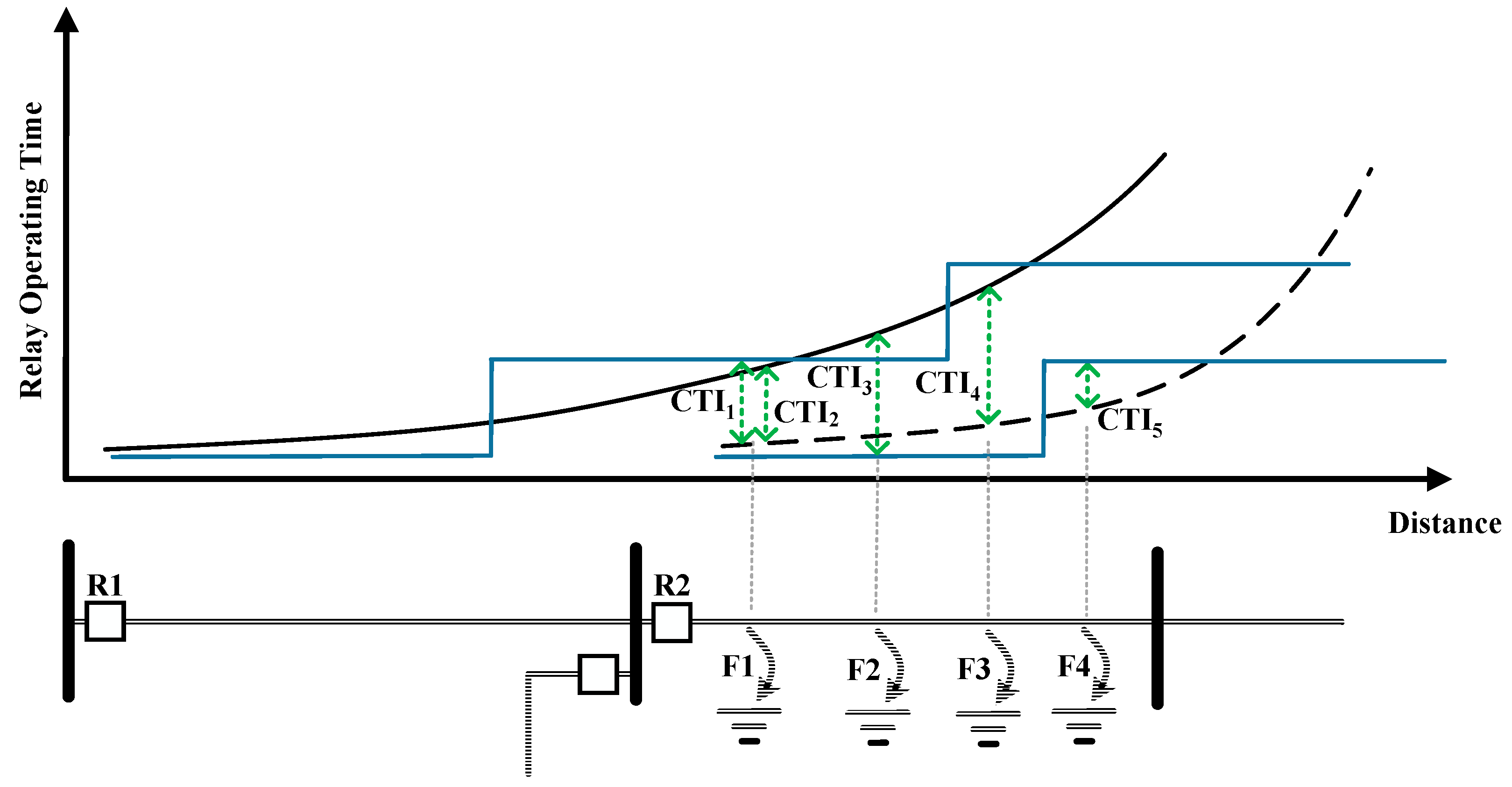
This subsection presents the problem formulation of the conventional DR–DOCR coordination based on the single-level relay characteristic [1,10,14]. This coordination scheme, including the relay operating characteristic curves, the fault locations, and CTI constraints, is illustrated in Figure 1. In the figure, the primary and backup relays are represented by R2 and R1, respectively. A total of five CTI constraints (CTI₁–CTI₅) are defined for four different fault locations (F1–F4). Among these, CTI₁, CTI₃, and CTI₅ represent the CTI constraints between the DOCRs and DRs, whereas CTI₂ and CTI₄ denote the CTI constraints between the DOCRs.

2.1.1. Objective Function

The objective function of the problem is defined as the sum of the primary and backup DOCR operating times, the Zone-2 operating times of the distance relay, and a penalty term incorporated to eliminate constraint violations. Accordingly, the objective function can be formulated as follows:

$$\mathrm{OF}={\mathrm{OF}}_1+{\mathrm{OF}}_2+Pen$$

(1)

where

$${\mathrm{OF}}_1=\sum _{\left(k,m\right)\in {\mathsf{\Omega }}_{RP}}\left(\sum _{f\in {\mathcal{F}}^{\mathrm{pri}}}\left(t_{pri,k,f}\right)+\sum _{g\in {\mathcal{F}}^{\mathrm{back}}}\left(t_{back,m,g}\right)\right)$$

(2)

$${\mathrm{OF}}_2=\sum _{d\in {\mathsf{\Omega }}_D}\left(t_{Z2,d}\right)$$

(3)

$$\begin{array}{c}Pen=PenCTI+PenT\\ PenCTI={\displaystyle \sum _{j=1}^{N_{RP}}\left[\sum _{c\in {\mathsf{\Omega }}_{\mathrm{CTI}}}{\delta }_1\times \max \left(0,{\mathrm{CTI}}_{\min }-{\mathrm{CTI}}_{j,c}\right)\right]}\\ PenT={\displaystyle \sum _{n=1}^{N_R}\left[\sum _{f\in {\mathcal{F}}^{\mathrm{pri}}}{\delta }_2\times \max \left(0,t_{\min }-t_{pri,n,f}\right)\right]}\end{array}$$

(4)

where $t_{pri,k,f}$ is the operating time of the primary DOCR $k$ obtained for fault location $f,$ while $t_{back,m,g}$ is the operating time of the backup DOCR $m$ obtained for fault location $g$. The sets ${\mathcal{F}}^{\mathrm{pri}}$ and ${\mathcal{F}}^{\mathrm{back}}$ represent the fault locations associated with the CTI constraints of the primary and backup DOCRs, respectively. Under Scenario 1, $\left\{\mathrm{F}1, \mathrm{F}3, \mathrm{F}4\right\}\in {\mathcal{F}}^{\mathrm{pri}}$ and $\left\{\mathrm{F}1, \mathrm{F}2, \mathrm{F}3\right\}\in {\mathcal{F}}^{\mathrm{back}}$. ${\mathsf{\Omega }}_{RP}$ denotes the set of DOCR pairs in the considered power system; $t_{Z2,d}$ indicates the Zone-2 operating time of distance relay $d$; ${\mathsf{\Omega }}_D$ represents the set of distance relays; ${\mathrm{CTI}}_{j,c}$ denotes the value of the $c$-th CTI constraint corresponding to the $j$-th relay pair; ${\mathrm{CTI}}_{\min }$ is the minimum CTI value (i.e., 0.2–0.5 s [37]); ${\mathsf{\Omega }}_{\mathrm{CTI}}$ represents the set of CTI constraints (CTI₁–CTI₅) illustrated in Figure 1; $N_{RP}$ is the number of relay pairs; $t_{\min }$ is the minimum DOCR operating time; $N_R$ represents the total number of DOCRs in the system; and ${\delta }_1$ and ${\delta }_2$ are the penalty coefficients with values of 500 and 1000, respectively.

According to IEC standards, the operating times of the primary and backup DOCRs are calculated using Equation (5) [12].

$$t_r={\mathrm{TDS}}_r\times {\displaystyle \frac{\alpha }{{\left(\raisebox{1ex}{$I_{f_{r,h}}$}\!\left/ \!\raisebox{-1ex}{${\mathrm{PS}}_r$}\right.\right)}^{\beta }-1}}$$

(5)

where ${\mathrm{TDS}}_r$ and ${\mathrm{PS}}_r$ denote the time dial setting and pickup setting values of DOCR $r$, respectively; $I_{f_{r,h}}$ represents the fault current flowing through the relay $r$ for a fault at location $h$; and $\alpha$ and $\beta$ are the relay characteristic coefficients with values of 0.14 and 0.02, respectively [8].

For the coordination problem addressed under Scenario 1, the decision variables are defined as given in Equation (6).

$${DV}_{scn1}=\left[\begin{array}{c}{\mathrm{TDS}}_r \forall k\in {\mathsf{\Omega }}_R\\ {\mathrm{PS}}_r \forall k\in {\mathsf{\Omega }}_R\\ t_{Z2,d} \forall d\in {\mathsf{\Omega }}_D\end{array}\right]$$

(6)

where ${\mathsf{\Omega }}_R$ denotes the set of DOCRs.

Accordingly, the decision variable vector for Scenario 1, ${DV}_{scn1}$, comprises the relay setting parameters of DOCRs and the Zone-2 operating time parameters of DRs, forming a unified optimization variable set for the DR–DOCR coordination problem. By solving the formulated optimization problem for Scenario 1, the optimal TDS and PS values of each DOCR, as well as the optimal Zone-2 operating time of each DR, $t_{Z2,d}$, are obtained.

2.1.2. Constraints

The problem constraints consist of the CTI constraints illustrated in Figure 1 and the constraints associated with the relay setting parameters that constitute the decision variables of the problem. For a selective protection coordination, the CTI must be maintained both between DOCRs themselves and between DOCRs and DRs. In this context, the CTI₁–CTI₅ constraints shown in Figure 1 are, respectively, given in Equations (7)–(11). At fault F1, there are two CTI constraints, CTI₁ and CTI₂. Equation (7), corresponding to CTI₁, denotes the CTI constraint between the primary DOCR and Zone-2 of the backup DR, while Equation (8), corresponding to CTI₂, represents the CTI constraint between the primary and backup DOCRs. At fault point F2, the CTI constraint between Zone-1 of the primary DR and the backup DOCR, denoted as CTI₃, is given in Equation (9). Equation (10) defines the CTI constraint between the primary and backup DOCRs at fault point F3. Lastly, Equation (11) corresponds to CTI₅, which denotes the CTI constraint between the primary DOCR and Zone-2 of the primary DR at fault point F4. On the other hand, the constraints related to $t_{Z2}$, $\mathrm{TDS}$ and $\mathrm{PS}$ relay setting parameters are provided in Equations (12)–(14), respectively.

$${\mathrm{CTI}}_{\min }\le t_{Z2,d}-t_{pri,k,\mathrm{F}1} \forall k\in {\mathsf{\Omega }}_R, \forall d\in {\mathsf{\Omega }}_D$$

(7)

$${\mathrm{CTI}}_{\min }\le t_{back,m,\mathrm{F}1}-t_{pri,k,\mathrm{F}1} \forall \left(k,m\right)\in {\mathsf{\Omega }}_{RP}$$

(8)

$${\mathrm{CTI}}_{\min }\le t_{back,m, \mathrm{F}2}-t_{Z1,y} \forall k\in {\mathsf{\Omega }}_R, \forall y\in {\mathsf{\Omega }}_D$$

(9)

$${\mathrm{CTI}}_{\min }\le t_{back,m,\mathrm{F}3}-t_{pri,k,\mathrm{F}3} \forall \left(k,m\right)\in {\mathsf{\Omega }}_{RP}$$

(10)

$${\mathrm{CTI}}_{\min }\le t_{Z2,y}-t_{pri,k,\mathrm{F}4} \forall k\in {\mathsf{\Omega }}_R,\forall y\in {\mathsf{\Omega }}_D$$

(11)

$$t_{Z2}^{\min }\le t_{Z2}\le t_{Z2}^{\max }$$

(12)

$${\mathrm{TDS}}^{\min }\le \mathrm{TDS}\le {\mathrm{TDS}}^{\max }$$

(13)

$${\mathrm{PS}}^{\min }\le \mathrm{PS}\le {\mathrm{PS}}^{\max }$$

(14)

where $t_{Z1,y}$ is the Zone-1 operating time of distance relay $y$. $t_{Z2}^{\min }$ and $t_{Z2}^{\max }$ represent the minimum and maximum bounds of the Zone-2 operating time of DRs, respectively. ${\mathrm{TDS}}^{\min }$ and ${\mathrm{TDS}}^{\max }$ denote the minimum and maximum bounds of the TDS values of DOCRs, respectively. ${\mathrm{PS}}^{\min }$ and ${\mathrm{PS}}^{\max }$ are the minimum and maximum bounds of the PS values of DOCRs, respectively.

Considering that the DR operates instantaneously in Zone-1 (i.e., with zero delay), a time delay is defined for the Zone-2 operating time of DRs, starting from 0.2 s, to allow the Zone-1 operation of nearby DRs to complete. In this study, $t_{Z2}^{\min }$ and $t_{Z2}^{\max }$ are set to 0.2 s and 5 s, respectively. ${\mathrm{TDS}}^{\min }$ and ${\mathrm{TDS}}^{\max }$ are generally determined based on the values specified by the relay manufacturer, and in this study, they are taken as 0.05 and 1.2, respectively. On the other hand, if the PS value is chosen lower than the maximum load current, the relays may sense normal operating currents as fault conditions; conversely, if it is set too high, actual fault currents may be perceived as normal operating conditions. In this study, ${\mathrm{PS}}^{\min }$ and ${\mathrm{PS}}^{\max }$ are selected as 1 and 1.5 times the maximum load current, respectively.

2.2. Scenario 2: The Proposed Two-Level DOCR-Based DR-DOCR Coordination Scheme

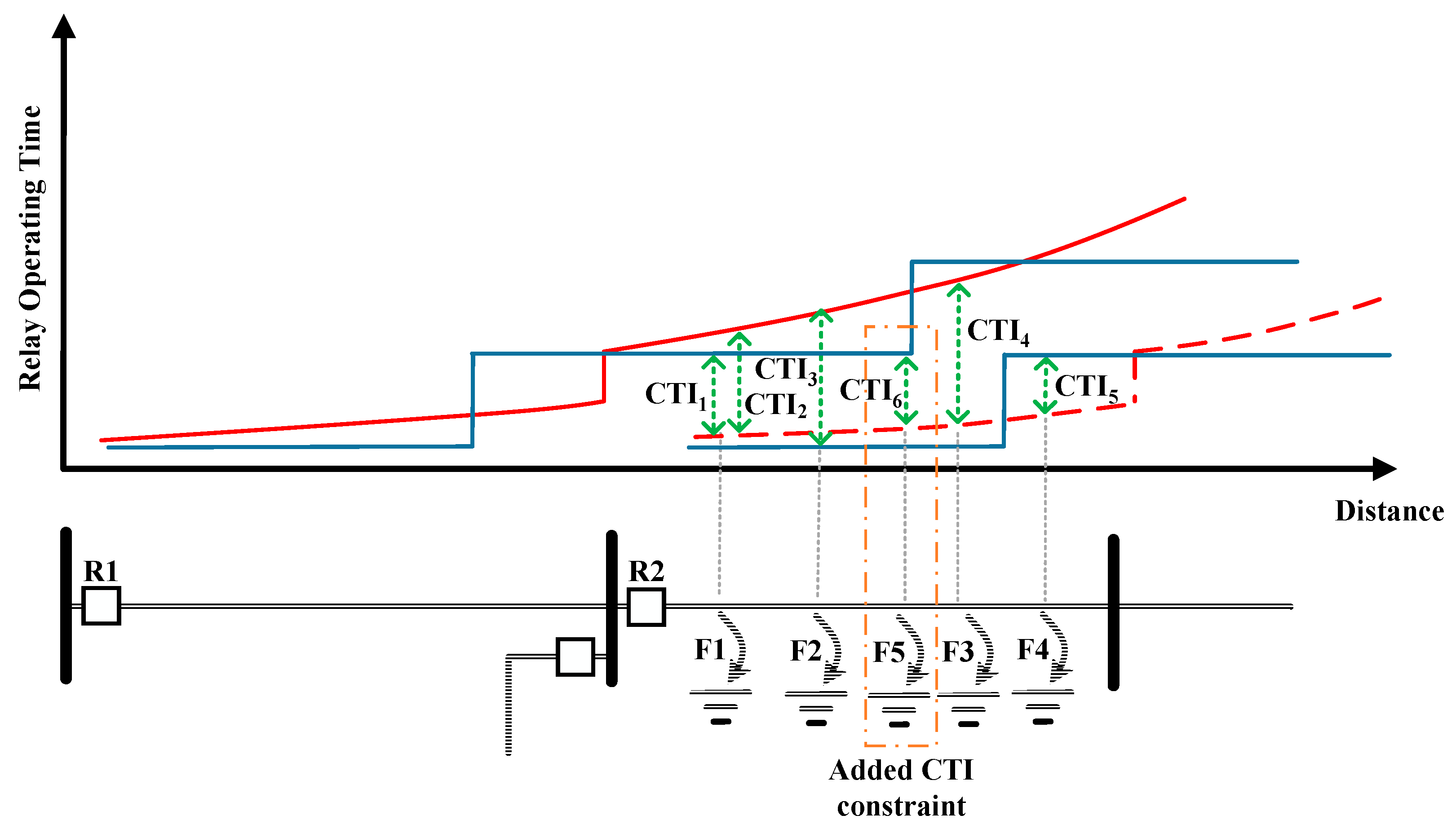
The representation of the proposed DR–DOCR coordination is illustrated in Figure 2. Within the scope of the proposed coordination scheme, the two-level relay characteristic presented in [18] is adapted for DR–DOCR coordination. Unlike the conventional single-level DOCR characteristic shown in Figure 1, the proposed method considers each DOCR to have a two-level structure, thereby enabling the assignment of distinct setting parameters to DOCRs for primary and backup protection duties. In addition, for the considered two-level DOCRs, the user-defined selection of the $\alpha$ and $\beta$ coefficients in Equation (5), together with the availability of a shift adjustment between the primary and backup relay characteristics, provides flexibility in the proposed coordination method. This flexibility helps avoid CTI violations and achieve lower relay operating times.

On the other hand, the proposed coordination scheme increases the number of considered fault locations to five (F1–F5) and the number of CTI violation constraints to six (CTI₁–CTI₆). The main motivation for this modification is that, in the region corresponding to fault point F5 in Figure 2, the Zone-2 curve of the backup DR and the curve of the primary DOCR become very close to each other, which may lead to a CTI violation in this region. This shortcoming observed in previous studies in the literature [1,10,14] is addressed within the scope of the proposed protection coordination scheme, thereby aiming to ensure a more secure and reliable protection coordination.

2.2.1. Relay Operating Time Calculation for Two-Level DOCRs

In the proposed protection coordination scheme, each DOCR can be assigned two distinct setting groups for primary and backup protection duties. In this context, the primary and backup operating times of the $r$-th DOCR are calculated using Equations (15) and (16), respectively.

$$t_{pri,r}={\mathrm{TDS}}_{r,1}\times {\displaystyle \frac{{\alpha }_{r,1}}{{\left(\raisebox{1ex}{$I_{f_{pri,r,h}}$}\!\left/ \!\raisebox{-1ex}{${\mathrm{PS}}_{r,1}$}\right.\right)}^{{\beta }_{r,1}}-1}}$$

(15)

$$t_{back,r}={\mathrm{TDS}}_{r,2}\times {\displaystyle \frac{{\alpha }_{r,2}}{{\left(\raisebox{1ex}{$I_{f_{back,r,h}}$}\!\left/ \!\raisebox{-1ex}{${\mathrm{PS}}_{r,2}$}\right.\right)}^{{\beta }_{r,2}}-1}}+t_r^{sh}$$

(16)

where $f_{pri,r,h}$ and $I_{f_{back,r,h}}$ denote the fault currents flowing through the $r$-th DOCR for primary and backup protection, respectively, and $t_r^{sh}$ represents the shift setting parameter of the $r$-th DOCR.

2.2.2. Extension of the Problem Constraints Considering the New Fault Location and Decision Variables

The CTI constraint (CTI₆) between the primary DOCR and the backup DR at the newly considered fault location in Figure 2 is given in Equation (17). In addition, the constraints associated with the additional setting parameters, which are used in the calculation of relay operating times in Equations (15) and (16) and define the user-defined and shift-based structure of the two-level DOCRs in the proposed relay coordination, are provided in Equations (18)–(20).

$${\mathrm{CTI}}_{\min }\le t_{Z2,d}-t_{pri,r,\mathrm{F}5} \forall r\in {\mathsf{\Omega }}_R, \forall d\in {\mathsf{\Omega }}_D$$

(17)

$${\alpha }^{\min }\le \alpha \le {\alpha }^{\max }$$

(18)

$${\beta }^{\min }\le \beta \le {\beta }^{\max }$$

(19)

$${t^{sh}}^{\min }\le t^{sh}\le {t^{sh}}^{\max }$$

(20)

2.2.3. The Coordination Problem for Scenario 2

For the proposed coordination scheme, the optimization problem is formulated as follows:

$$\begin{array}{c} \mathrm{Minimize} OF:\mathrm{Equation}(1)\\ \mathrm{Subject} \mathrm{to} \left\{\begin{array}{c}\mathrm{O}\mathrm{p}\mathrm{e}\mathrm{r}\mathrm{a}\mathrm{t}\mathrm{i}\mathrm{n}\mathrm{g} \mathrm{t}\mathrm{i}\mathrm{m}\mathrm{e} \mathrm{e}\mathrm{q}\mathrm{u}\mathrm{a}\mathrm{t}\mathrm{i}\mathrm{o}\mathrm{n}\mathrm{s}: \mathrm{E}\mathrm{q}\mathrm{u}\mathrm{a}\mathrm{t}\mathrm{i}\mathrm{o}\mathrm{n}\mathrm{s} \left(15\right) \mathrm{a}\mathrm{n}\mathrm{d} \left(16\right) \\ \mathrm{C}\mathrm{T}\mathrm{I} \mathrm{c}\mathrm{o}\mathrm{n}\mathrm{s}\mathrm{t}\mathrm{r}\mathrm{a}\mathrm{i}\mathrm{n}\mathrm{t}\mathrm{s}: \mathrm{E}\mathrm{q}\mathrm{u}\mathrm{a}\mathrm{t}\mathrm{i}\mathrm{o}\mathrm{n}\mathrm{s} \left(7\right)–\left(11\right) \mathrm{a}\mathrm{n}\mathrm{d} \left(17\right) \\ \mathrm{R}\mathrm{e}\mathrm{l}\mathrm{a}\mathrm{y} \mathrm{s}\mathrm{e}\mathrm{t}\mathrm{t}\mathrm{i}\mathrm{n}\mathrm{g} \mathrm{c}\mathrm{o}\mathrm{n}\mathrm{s}\mathrm{t}\mathrm{r}\mathrm{a}\mathrm{i}\mathrm{n}\mathrm{t}\mathrm{s}: \mathrm{E}\mathrm{q}\mathrm{u}\mathrm{a}\mathrm{t}\mathrm{i}\mathrm{o}\mathrm{n}\mathrm{s} \left(12\right)–\left(14\right) \mathrm{a}\mathrm{n}\mathrm{d} \left(18\right)–\left(20\right)\\ \left\{\mathrm{F}1, \mathrm{F}3, \mathrm{F}4, \mathrm{F}5\right\}\in {\mathcal{F}}^{\mathrm{pri}} \mathrm{a}\mathrm{n}\mathrm{d} \left\{\mathrm{F}1, \mathrm{F}2, \mathrm{F}3\right\}\in {\mathcal{F}}^{\mathrm{back}} \end{array}\right.\end{array}$$

(21)

The decision variables of the optimization problem are defined as given in Equation (22).

$${DV}_{scn2}=\left[\begin{array}{c}\begin{array}{c}\begin{array}{c}{\mathrm{TDS}}_{r,1} \forall r\in {\mathsf{\Omega }}_R\\ {\mathrm{PS}}_{r,1} \forall r\in {\mathsf{\Omega }}_R\\ {\alpha }_{r,1} \forall r\in {\mathsf{\Omega }}_R\end{array}\\ {\beta }_{r,1} \forall r\in {\mathsf{\Omega }}_R\end{array}\\ {\mathrm{TDS}}_{r,2} \forall r\in {\mathsf{\Omega }}_R\\ {\mathrm{PS}}_{r,2} \forall r\in {\mathsf{\Omega }}_R\\ {\alpha }_{r,2} \forall r\in {\mathsf{\Omega }}_R\\ {\beta }_{r,2} \forall r\in {\mathsf{\Omega }}_R\\ t_{Z2,\mathrm{d}} \forall d\in {\mathsf{\Omega }}_D\\ t_r^{sh} \forall r\in {\mathsf{\Omega }}_R\end{array}\right]$$

(22)

As seen in Equation (22), there are totally ten different decision variables within Scenario 2. Unlike Scenario 1, where each relay has a single TDS and PS value, in Scenario 2, each DOCR is assigned separate TDS and PS values for its primary and backup protection functions. Furthermore, the values of $\mathit{\alpha }$ and $\mathit{\beta }$, which are taken as fixed in Scenario 1, are considered as decision variables in the optimization problem in Scenario 2, i.e., as user-defined relay setting parameters. In this context, the optimized values of ${\mathrm{TDS}}_{\mathit{r},1}$, ${\mathrm{PS}}_{\mathit{r},1}$, ${\mathit{\alpha }}_{\mathit{r},1}$, and ${\mathit{\beta }}_{\mathit{r},1}$ determine the lower portion of the DOCR characteristic corresponding to relay’s primary protection function in Figure 2, while the values of ${\mathrm{TDS}}_{\mathit{r},2}$, ${\mathrm{PS}}_{\mathit{r},2}$, ${\mathit{\alpha }}_{\mathit{r},2}$, and ${\mathit{\beta }}_{\mathit{r},2}$ define the upper portion of the DOCR curve for the backup protection task. The level of separation between the lower and upper curves in this split characteristic is determined by the shift parameter ${\mathit{t}}_{\mathit{r}}^{\mathit{s}\mathit{h}}$. In this way, by splitting the DOCRs into primary and backup characteristic curves under Scenario 2, the relay operating times can be obtained at lower values, while the CTI violations can be easily overcome. Accordingly, the proposed method allows for greater flexibility in the relay characteristics by utilizing the numerous decision variables given in Equation (22), and it is expected to achieve lower relay operating times compared to conventional coordination approach.

3. Enhanced Red-Tailed Hawk Algorithm

This paper proposes an enhanced red-tailed hawk algorithm (ERTH) to solve the DR–DOCR coordination problem described in Section 2. In this context, the present section first introduces the original RTH algorithm and then details the mathematical modifications and structural improvements incorporated into the proposed ERTH algorithm.

3.1. The Original RTH Algorithm

The RTH algorithm is a metaheuristic optimization algorithm inspired by the hunting behavior of red-tailed hawks. Red-tailed hawks are carnivorous birds of prey commonly found in regions such as Alaska, Canada, Panama, and the West Indies. Unlike many other hawk species, red-tailed hawks conserve energy by minimizing wing flapping and gliding with a dihedral wing angle, enabling them to travel longer distances efficiently. Rodents constitute the largest portion of their diet; however, they also prey on fish, birds, and reptiles. During gliding, red-tailed hawks can reach speeds of 32–64 km/h, while during diving their speed can increase up to 190 km/h [24].

The hunting behavior of red-tailed hawks consists of three main phases—high soaring, low soaring, and swooping—which form the search mechanism of the RTH optimization algorithm. Prior to these phases, the optimization process begins with the random initialization of the population individuals. The equation corresponding to this initialization phase is given in Equation (23).

$$X_i^0=p_3\times \left(ub-lb\right)+lb$$

(23)

where the vectors $ub$ and $lb$ are the upper and lower bound values of the decision variables, respectively, and $p_3$ represents a random number between 0 and 1.

3.1.1. High Soaring

In the RTH algorithm, the position update of individuals during the high-soaring phase is computed using Equation (24). In this phase, red-tailed hawks fly at high altitudes to identify suitable hunting areas. Here, this high-altitude flight actually corresponds to the exploration stage of the optimization process. In this stage, the search space is explored broadly by the algorithm, and promising regions in the search space are attempted to be discovered.

$$X_i^{t+1}=X_{best}^t+\left(X_{mean}^t-X_i^t\right)\times Levy\left(\mathrm{D}\right)\times {TF}^t$$

(24)

where $X_i^t$ and $X_i^{t+1}$ are the current and next-iteration positions of the $i$-th individual, respectively, while $X_{best}^t$ and $X_{mean}^t$ represent the position of the best individual and the mean position vector of the individuals in the population, respectively. $Levy\left(\mathrm{D}\right)$ represents the Lévy flight distribution function and is calculated according to Equation (25).

$$\begin{array}{c}Levy(\mathrm{D})=c_1{\displaystyle \frac{\mu \times \sigma }{{\left|\nu \right|}^{{\delta }^{-1}}}}\\ \sigma =\left({\displaystyle \frac{\mathsf{\Gamma }\left(1+\delta \right)\times \mathrm{s}\mathrm{i}\mathrm{n}\left(\frac{\pi \delta }{2}\right)}{\mathsf{\Gamma }\left(\frac{1+\delta }{2}\right)\times \delta \times 2^{\left(\frac{1-\delta }{2}\right)}}}\right)\end{array}$$

(25)

where $\mathrm{D}$ denotes the problem dimension. The parameters $\mu$ and $\nu$ are random numbers uniformly distributed between 0 and 1, while $c_1$ and $\delta$ are constant parameters with values of 0.01 and 1.5, respectively.

On the other hand, the term ${TF}^t$ in Equation (24) denotes the transition factor function, which is defined as follows:

$${TF}^t=1+\mathrm{s}\mathrm{i}\mathrm{n}(2.5+{\displaystyle \frac{t}{{\mathrm{T}}_{max}}})$$

(26)

where ${\mathrm{T}}_{max}$ is the maximum number of iterations.

3.1.2. Low Soaring

In the low-soaring phase, red-tailed hawks descend toward the food-rich locations identified during the previous high-soaring phase and perform close-range flights around their prey to determine the optimal moment for attack. Within the optimization framework, this process can be considered as the transition phase between the exploration and exploitation stages. In this transition phase, the algorithm tends to search for promising regions in the search space in order to reach the global optimum, while simultaneously performing local searches.

The low-soaring behavior of red-tailed hawks is modeled in the RTH algorithm as expressed in Equation (27).

$$X_i^{t+1}=X_{best}^t+\left(a_i^t+b_i^t\right)\times \left(X_i^{t+1}-X_{mean}^t\right)$$

(27)

where $a_i^t$ and $b_i^t$ express the directional coordinates and are calculated as follows:

$$\left\{\begin{array}{c}{a}_i^t=R_i^t\times sin\left({\theta }_i^t\right)\\ b_i^t=R_i^t\times cos\left({\theta }_i^t\right)\end{array}\right. \left\{\begin{array}{c}{R}_i^t=R_0\times e_1\times \left(ro-{\displaystyle \frac{t}{{\mathrm{T}}_{max}}}\right)\\ {\theta }_i^t=A\times e_2\times \left(1-{\displaystyle \frac{t}{{\mathrm{T}}_{max}}}\right)\end{array}\right.\left\{\begin{array}{c}{a}_i^t={\displaystyle \frac{a_i^t}{max\left|a^t\right|}}\\ b_i^t={\displaystyle \frac{b_i^t}{max\left|b^t\right|}}\end{array}\right.$$

(28)

where $e_1$ and $e_2$ represent random numbers varying between 0 and 1. The parameters $R_0$, $A$, and $ro$ denote the control parameters of the RTH algorithm, whose values vary within the ranges of 0.1–2, 5–25, and 0.1–2, respectively [24].

3.1.3. Swooping

In this phase, red-tailed hawks initiate a sudden attack toward the prey from the best position identified during the low-soaring stage. Algorithmically, the process corresponds to the exploitation phase. Rather than performing large-scale searches across the entire search space, it focuses on intensively searching within a limited region in the search space to achieve the best possible solution.

The position update in the swooping phase is performed according to Equation (29).

$$\begin{array}{c}{X}_i^{t+1}={\tau }_i^t\times X_{best}^t+a_i^t\times {Step1}^t+b_i^t\times {Step2}^t\\ {\tau }_i^t={\mathrm{s}\mathrm{i}\mathrm{n}}^2(2.5-{\displaystyle \frac{t}{{\mathrm{T}}_{max}}})\\ \begin{array}{c}{Step1}^t=X_i^t-{TF}^t\times X_{mean}^t\\ {Step2}^t=G_i^t\times X_i^t-{TF}^t\times X_{best}^t\end{array}\\ G_i^t=2\times (1-{\displaystyle \frac{t}{{\mathrm{T}}_{max}}})\end{array}$$

(29)

3.2. The Proposed ERTH Algorithm

In this study, the ERTH algorithm is proposed to solve the optimal DR-DOCR coordination problem. The ERTH algorithm is designed to enhance the exploration capability of the original RTH algorithm and establish a strong exploration–exploitation balance, thereby preventing it from being trapped in local optima. The ERTH algorithm is derived from the original RTH framework through three enhancements detailed below: chaotic initialization, effective tracking of the best individual and its neighborhood, and a diversity enhancement strategy based on the differential evolution algorithm.

3.2.1. Chaotic Initialization

In metaheuristic optimization algorithms, the optimization process is generally initiated by assigning random positions to individuals. However, due to this random assignment, individuals may fail to achieve a well-distributed coverage of the search space. Because of randomness, some individuals may be located close to each other, leading to promising regions of the search space being overlooked. To overcome these drawbacks, recent studies in the literature have increasingly preferred chaotic initialization procedures instead of random position assignment [38]. Chaotic initialization enables a more comprehensive and well-distributed placement of individuals across the search space at the beginning of the optimization process. For this reason, in the ERTH algorithm, the initial positions of individuals are determined using a chaotic initialization procedure instead of the random initialization employed in the original RTH algorithm. Among the commonly used chaotic maps in the literature, the logistic map, whose mathematical model is given in Equation (30), is adopted for the applied chaotic initialization procedure.

$$z_{i+1}=\lambda z_i\left(1-z_i\right)$$

(30)

where $\lambda$ is a control parameter that takes values in the range of 3.8 to 4, and it is set to 4 in this study. The initial state variable, $z_1$, is considered a random number within the interval of 0 to 1. Accordingly, the initial positions of the population individuals are obtained as follows:

$$X_i^0=z_i\times \left(ub-lb\right)+lb$$

(31)

3.2.2. Effective Tracking of the Best Individual and Its Neighborhood

The position of the best individual significantly influences the hunting or food-searching behavior of the other individuals. Incorporating the best individual’s position into the swarm’s position update mechanism enables individuals to move away from ineffective regions of the search space and toward promising areas, thereby allowing them to search more efficiently for better solutions. As a result of this behavior, the convergence performance of the algorithm can also be improved. However, a critical point is that individuals are expected to gradually shift their focus toward the best individual. Otherwise, if the swarm members concentrate on the best individual at the early stages of the optimization process, other potentially effective regions may be overlooked. On the other hand, an effective exploration of the neighborhood of the best individual increases the likelihood that other swarm members will also identify better solutions around it. Accordingly, the position update rule given in Equation (32) is incorporated into the ERTH algorithm to ensure the effective tracking of the best individual and its neighborhood.

$$Y_i^t=\left\{\begin{array}{c}{\omega X}_i^t+r_1\times \left(X_{best}^t-X_i^t\right), if p_1>0.5\\ X_{best}^t+r_2\times s_1\times {\displaystyle \frac{t}{{\mathrm{T}}_{max}}}, \mathrm{o}\mathrm{t}\mathrm{h}\mathrm{e}\mathrm{r}\mathrm{w}\mathrm{i}\mathrm{s}\mathrm{e} \end{array}\right.$$

(32)

where the parameters $r_1$, $r_2$, and $p_1$ are random numbers uniformly distributed in the range of 0 to 1, whereas $s_1$ is a random number within the interval of −2 to 2. The parameter $\omega$, similar to the inertia weight in the PSO algorithm, controls the tendency of an individual to follow the best individual. In the ERTH algorithm, the value of $\omega$ decreases iteratively as follows:

$$\omega =1-{\displaystyle \frac{t}{{\mathrm{T}}_{max}}}$$

(33)

To prevent individuals from losing their current positions against moving away from promising regions while following the best individual and its neighborhood, and to enhance their foraging efficiency, the next position is determined based on a comparison between the trial position, $Y_i^t$, obtained at this stage of the optimization process and the current position, $X_i^t$, as follows:

$$X_i^{t+1}=\left\{\begin{array}{c}{Y}_i^t, if f\left(Y_i^t\right) < f\left(X_i^t\right) \\ X_i^t, \mathrm{o}\mathrm{t}\mathrm{h}\mathrm{e}\mathrm{r}\mathrm{w}\mathrm{i}\mathrm{s}\mathrm{e} \end{array}\right.$$

(34)

3.2.3. Diversity Enhancement Strategy Based on the Differential Evolution Algorithm

A well-designed metaheuristic algorithm is expected to explore regionally promising areas of the search space during the initial iterations and, in the subsequent iterations, to focus on these regions, enabling convergence toward near–global optimal solutions through an effective exploitation process. However, the optimization process does not always progress in this manner, and algorithms may become trapped in local optima. In this context, maintaining diversity among individuals is essential for effectively exploring the search space without premature convergence. In this study, to preserve population diversity, the mutation, crossover, and selection mechanisms of the differential evolution (DE) algorithm are incorporated into the ERTH algorithm.

Mutation Operator: The mutation operation used to generate the mutant position vector $V_i^t$ is performed as follows:

$$V_i^t=X_{best}^t+\mathrm{F}\times \left(X_{r1}^t-X_{r2}^t\right)$$

(35)

where $X_{r1}^t$ and $X_{r2}^t$ represent the positions of two individuals randomly selected from the population. The parameter $\mathrm{F}$, set to 0.5, is a control factor that scales the difference between the position vectors of these randomly selected individuals.

Crossover Operator: After obtaining the mutant vector, a crossover operation is applied in the second phase. Based on the position vectors $X_i^t$ and $V_i^t$, the trial vector $U_i^t$ is generated as follows:

$$U_{i,j}^t=\left\{\begin{array}{c}{V}_{i,j}^t, if p_{2,j}\le \mathrm{C}\mathrm{R} \mathrm{o}\mathrm{r} (j\in {\mathsf{\Omega }}_{\mathrm{CR}})\\ X_{i,j}^t, \mathrm{o}\mathrm{t}\mathrm{h}\mathrm{e}\mathrm{r}\mathrm{w}\mathrm{i}\mathrm{s}\mathrm{e} \end{array}\right.$$

(36)

where $V_{i,j}^t$ denotes the value of the mutation vector in the $j$th dimension. The variable $p_{2,j}$ is a random number uniformly distributed between 0 and 1, and $\mathrm{CR}$, set to 0.5, represents the crossover control parameter. The set ${\mathsf{\Omega }}_{\mathrm{CR}}$ denotes the indices of the vector dimensions selected randomly for crossover. In this study, the number of randomly selected indices in the ${\mathsf{\Omega }}_{\mathrm{CR}}$ is taken as one-fifth of the total problem dimension based on the trial-and-error procedure.

Selection: In the final stage, the next generation vector is determined by comparing the trial vector $U_i^t$ with the current position vector $X_i^t$, similarly to Equation (34). Accordingly, the position vector for the next generation is defined as given in Equation (37), depending on whether $U_i^t$ provides a better solution than $X_i^t$.

$$X_i^{t+1}=\left\{\begin{array}{c}{U}_i^t, if f\left(U_i^t\right) < f\left(X_i^t\right) \\ X_i^t, \mathrm{o}\mathrm{t}\mathrm{h}\mathrm{e}\mathrm{r}\mathrm{w}\mathrm{i}\mathrm{s}\mathrm{e} \end{array}\right.$$

(37)

3.2.4. Workflow of the ERTH Algorithm

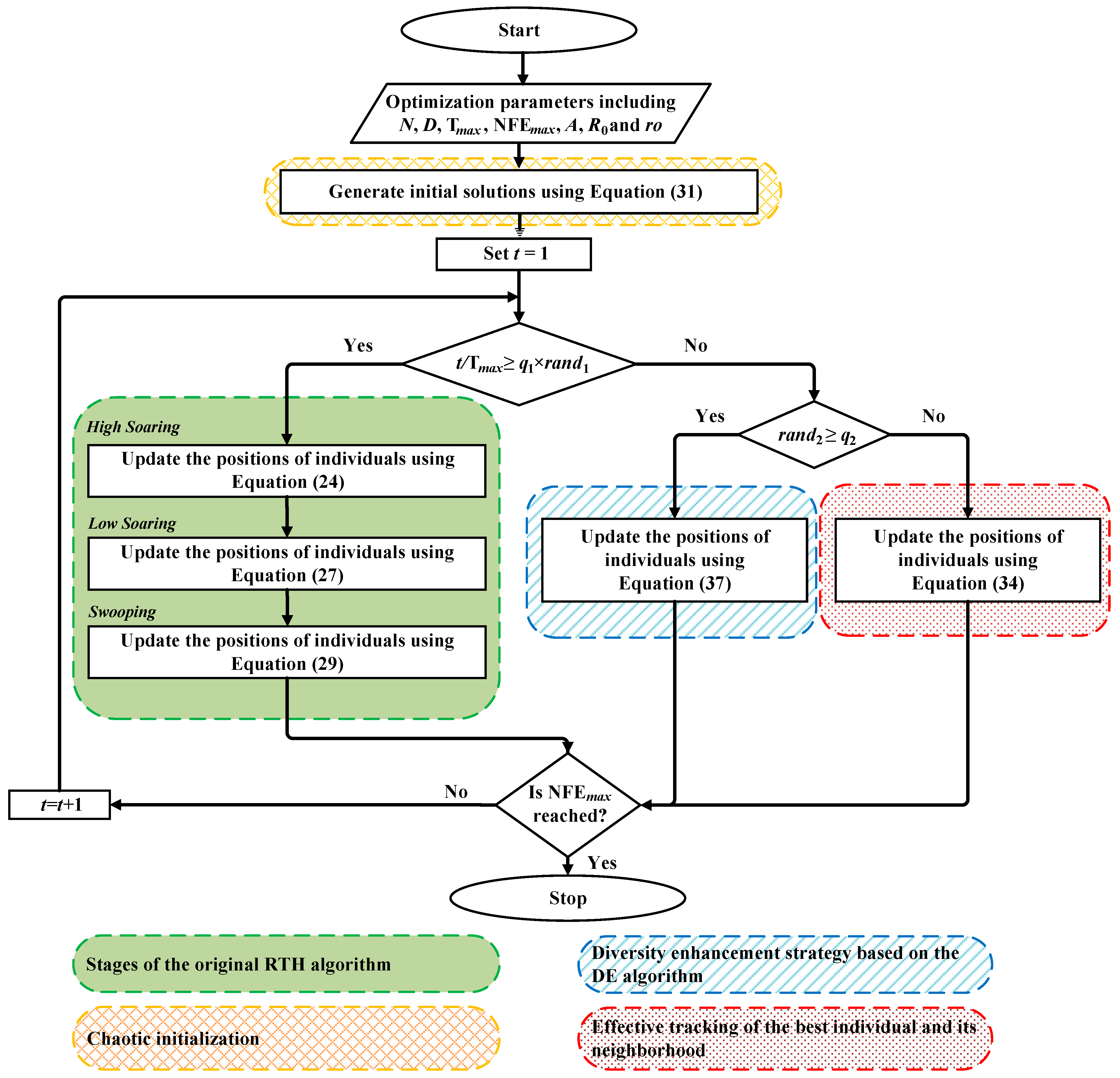
The flowchart of the IRTH algorithm is presented in Figure 3. In the initial stage, the initial positions of individuals are determined according to the chaotic initialization procedure using the formulation given in Equation (31). Then, the transition between the original RTH algorithm stages and the newly incorporated stages of the ERTH algorithm is controlled by the condition $t/{\mathrm{T}}_{max}\ge$ q₁ $\times$ rand₁. If this condition is satisfied, the optimization process continues based on the stages of the original RTH algorithm. Otherwise, the algorithm proceeds with the newly introduced stages of the ERTH algorithm. At this point, the stage to be used for updating the positions of individuals is determined by the condition rand₂ $\ge$ q₂. If the condition rand₂ $\ge$ q₂ is satisfied, the positions of individuals are updated according to Equation (37); otherwise, they are updated using Equation (34). Here, rand₁ and rand₂ denote random numbers uniformly distributed between 0 and 1, while q₁ and q₂ are control parameters determined through a trial-and-error procedure and set to 0.25 and 0.8, respectively.

As the termination criterion of the algorithm, the maximum number of function evaluations (${\mathrm{N}\mathrm{F}\mathrm{E}}_{max}$) is employed. During the iterative process, the algorithm stops when ${\mathrm{N}\mathrm{F}\mathrm{E}}_{max}$ is reached; otherwise, the iteration counter is increased, and the optimization process continues.

4. Simulation Results

The proposed method is implemented on the modified versions of the 8-bus and the 33 kV portion of the 30-bus test systems. For the experiments conducted on these power systems, both Scenario 1 and Scenario 2, described in Section 2, are considered. Load and fault currents seen by the relays are obtained using DIgSILENT PowerFactory. The bounds of the decision variables for Scenarios 1 and 2 are presented in

Table 2. The upper and lower bounds on relay settings for Scenario 1.

${\mathbf{TDS}}_{\mathit{r}}$	${\mathbf{PS}}_{\mathit{r}}$	${\mathit{t}}_{\mathit{Z}\mathbf{2},\mathit{d}}$ (s)
0.05–1.2	1 × ${\mathrm{I}}_{\mathrm{L}\mathrm{m}\mathrm{a}\mathrm{x}}$–1.5 × ${\mathrm{I}}_{\mathrm{L}\mathrm{m}\mathrm{a}\mathrm{x}}$	0.2–5

and

Table 3. The upper and lower bounds on relay settings for Scenario 2.

${\mathbf{TDS}}_{\mathit{r},\mathbf{1}}$	${\mathbf{PS}}_{\mathit{r},\mathbf{1}}$	${\mathit{\alpha }}_{\mathit{r},\mathbf{1}}$	${\mathit{\beta }}_{\mathit{r},\mathbf{1}}$	${\mathbf{TDS}}_{\mathit{r},\mathbf{2}}$	${\mathbf{PS}}_{\mathit{r},\mathbf{2}}$	${\mathit{\alpha }}_{\mathit{r},\mathbf{2}}$	${\mathit{\beta }}_{\mathit{r},\mathbf{2}}$	${\mathit{t}}_{\mathit{Z}\mathbf{2},\mathit{d}}$ (s)	${\mathit{t}}_{\mathit{r}}^{\mathit{s}\mathit{h}}$ (s)
0.05–1.2	$1 \times {\mathrm{I}}_{\mathrm{L}\mathrm{m}\mathrm{a}\mathrm{x}}$$–1.5 \times {\mathrm{I}}_{\mathrm{L}\mathrm{m}\mathrm{a}\mathrm{x}}$	0.14–80	0.02–2	0.05–1.2	$1 \times {\mathrm{I}}_{\mathrm{L}\mathrm{m}\mathrm{a}\mathrm{x}}$$–1.5 \times {\mathrm{I}}_{\mathrm{L}\mathrm{m}\mathrm{a}\mathrm{x}}$	0.14–80	0.02–2	0.2–5	0.001–5

, respectively. The coordination design parameters, namely the minimum operating time of the DOCRs ($t_{\min }$) and the minimum coordination time interval (${\mathrm{CTI}}_{\min }$), are set to 0.05 and 0.2 s, respectively. Due to the instantaneous operating characteristic of DRs in Zone-1, the operating time is taken as $t_{Z1,y}$ = 0.

On the other hand, to evaluate the performance of the ERTH algorithm, in addition to ERTH, the APO, EEFO, EEO, GJO, GWO, HBA, JS, KOA, MSA, PSO, TLBO, and the original RTH algorithms are also employed to solve the problem, and the obtained results are presented comparatively in this section. Among the comparison algorithms, as shown in Table 1, GWO, EEO, and TLBO have been previously proposed in the literature for solving the optimal DR–DOCR coordination problem. The parameter settings of these algorithms, along with their corresponding values, are presented in

Table 4. Parameter settings of comparison algorithms.

Algorithm	Year	Control Parameter	Value
APO [27]	2024	F, C	0.5, 0.5
EEFO [28]	2024	-	-
EEO [14]	2024	a1, a2, GP	$2-2 \times (t/({\mathrm{T}}_{max}-t))$, 1, exp $(-($4 × $t/({\mathrm{T}}_{max}-t\left){)}^2\right)$
GJO [29]	2022	C1	2
GWO [30]	2014	a	$2-2 \times \left(t/{\mathrm{T}}_{max}\right)$
HBA [31]	2022	C, $\beta$	2, 6
JS [32]	2021	-	-
KOA [33]	2023	$\overline{T}$, ${\mu }_0$, γ	3, 0.1, 1.5
MSA [34]	2023	A, $a$, $P_c$, $\rho$, $p$, $P$	1, 0.5, 0.2, 6, 0.5, 2
PSO [35]	1995	$c_1$, $c_2$, $w$	1.5, 1.5, 0.9
TLBO [36]	2011	-	-
RTH [24]	2023	$R_0$, $A$, $ro$	0.5, 15, 1.5
ERTH	Present	$R_0$, $A$, $ro$, $\mathrm{F}$, CR, $\omega$	0.5, 15, 1.5, 0.5, 0.5, 1$-t/{\mathrm{T}}_{max}$

. All simulation experiments are performed using MATLAB R2025b through a personal computer with 8 GB RAM and 2.7 GHz CPU speed. The population size is 500, and ${\mathrm{N}\mathrm{F}\mathrm{E}}_{max}$ is set to 500,000 and 1,000,000 for the 8-bus and 30-bus systems, respectively. Due to the stochastic nature of metaheuristic optimization algorithms, each algorithm is run 20 times independently.

4.1. 8-Bus Test System

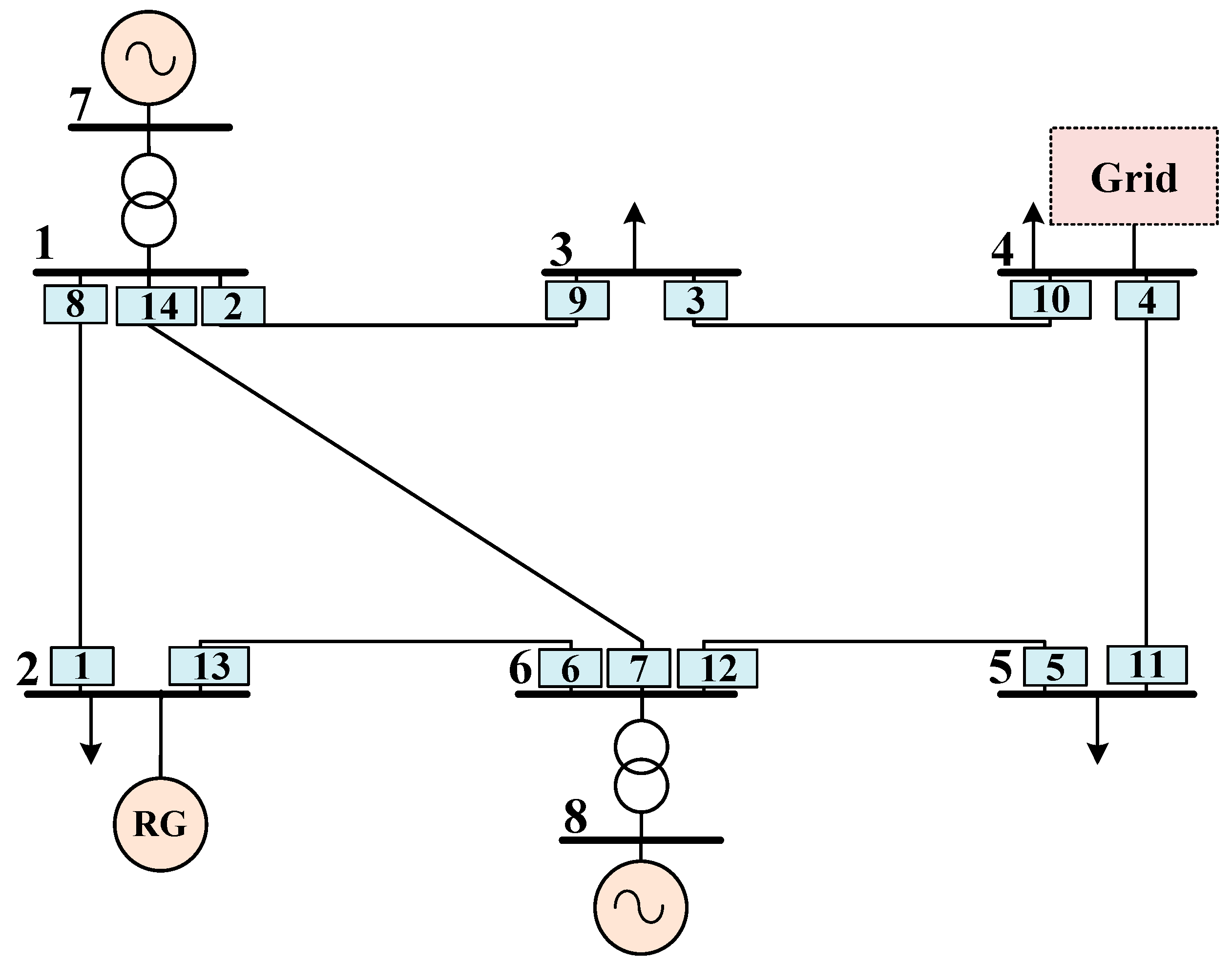
The single-line diagram of the modified 8-bus power system is shown in Figure 4. In this system, unlike the benchmark model, a 20-MW renewable energy source is assumed to be connected to bus no. 2 to reflect the structure of modern power systems. As mentioned before, since most renewable energy sources are inverter-interfaced, their contributions to fault currents are limited. Therefore, the fault current contribution from the renewable energy source is neglected in this study. However, the integration and disconnection of this source may significantly affect the system load currents [3]. In this context, the maximum load currents flowing through the relays (${\mathrm{I}}_{\mathrm{L}\mathrm{m}\mathrm{a}\mathrm{x}}$) are calculated by considering both operating conditions of the source, i.e., when it is in service and out of service.

On the other hand, as shown in Figure 4, the 8-bus test system includes a total of 14 relay locations at the sending and receiving ends of each transmission line and 20 relay pairs [39].

For the 8-bus power system under Scenario 1, the optimal DR and DOCR settings obtained using the ERTH algorithm are presented in

Table 5. Optimal relay settings obtained using the ERTH algorithm for the 8-bus system under Scenario 1.

Relay No.	${\mathbf{TDS}}_{\mathit{r}}$	${\mathbf{PS}}_{\mathit{r}}$	${\mathit{t}}_{\mathit{Z}\mathbf{2},\mathit{d}}$
1	0.322	102.072	1.111
2	0.279	512.603	1.159
3	0.427	90.362	1.083
4	0.306	103.053	0.857
5	0.092	569.120	1.047
6	0.400	123.000	1.016
7	0.658	20.346	1.154
8	0.391	131.688	1.034
9	0.103	515.502	1.057
10	0.309	108.154	0.866
11	0.420	103.052	1.094
12	0.274	560.792	1.167
13	0.320	106.296	1.130
14	0.670	20.044	1.165
OF(s)	120.702

. The relay operating times and the corresponding CTI values for these settings are given in

Table 6. Relay operating times and the CTIs for the DOCR-DOCR coordination using ERTH for the 8-bus system under Scenario 1.

Primary Relay	Backup Relay	Fault F1			Fault F3
		${\mathit{t}}_{\mathit{p}\mathit{r}\mathit{i}}$	${\mathit{t}}_{\mathit{b}\mathit{a}\mathit{c}\mathit{k}}$	CTI2	${\mathit{t}}_{\mathit{p}\mathit{r}\mathit{i}}$	${\mathit{t}}_{\mathit{b}\mathit{a}\mathit{c}\mathit{k}}$	CTI4
1	6	0.632	0.833	0.200	0.664	0.877	0.213
2	1	0.775	0.975	0.200	0.812	1.054	0.242
2	7	0.775	0.975	0.200	0.812	1.014	0.202
3	2	0.782	0.982	0.200	0.801	1.028	0.227
4	3	0.579	0.779	0.200	0.594	0.798	0.204
5	4	0.454	0.667	0.214	0.492	0.692	0.200
6	5	0.690	0.956	0.266	0.715	1.204	0.489
6	14	0.690	0.996	0.306	0.715	1.062	0.347
7	5	0.787	0.987	0.200	0.813	1.564	0.751
7	13	0.787	1.026	0.239	0.813	1.454	0.641
8	7	0.688	0.981	0.293	0.716	1.054	0.339
8	9	0.688	0.976	0.288	0.716	1.238	0.523
9	10	0.466	0.677	0.212	0.504	0.704	0.200
10	11	0.588	0.788	0.200	0.603	0.808	0.205
11	12	0.788	0.988	0.200	0.808	1.036	0.228
12	13	0.790	0.990	0.200	0.826	1.064	0.238
12	14	0.790	0.990	0.200	0.826	1.026	0.200
13	8	0.652	0.852	0.200	0.684	0.897	0.213
14	1	0.800	1.008	0.208	0.826	1.408	0.581
14	9	0.800	1.000	0.200	0.826	1.513	0.687

and

Table 7. Relay operating times and the CTIs for the DR-DOCR coordination using ERTH for the 8-bus system under Scenario 1.

Primary Relay	Backup Relay	Fault F1	Fault F2	Fault F4
		CTI1	${\mathit{t}}_{\mathit{b}\mathit{a}\mathit{c}\mathit{k}}$/CTI3	${\mathit{t}}_{\mathit{p}\mathit{r}\mathit{i}}$	CTI5
1	6	0.383	0.854	0.911	0.200
2	1	0.337	1.013	0.959	0.200
2	7	0.380	0.994	0.959	0.200
3	2	0.377	1.005	0.883	0.201
4	3	0.505	0.788	0.656	0.201
5	4	0.404	0.679	0.841	0.205
6	5	0.357	1.067	0.814	0.201
6	14	0.475	1.027	0.814	0.201
7	5	0.259	1.202	0.949	0.205
7	13	0.343	1.177	0.949	0.205
8	7	0.466	1.015	0.832	0.203
8	9	0.369	1.092	0.832	0.203
9	10	0.400	0.690	0.857	0.200
10	11	0.507	0.798	0.666	0.200
11	12	0.379	1.012	0.892	0.202
12	13	0.340	1.025	0.965	0.201
12	14	0.375	1.008	0.965	0.201
13	8	0.382	0.873	0.930	0.200
14	1	0.311	1.151	0.965	0.200
14	9	0.257	1.198	0.965	0.200

for DOCR–DOCR and DR–DOCR coordination, respectively. Since the DR operating times for the DR–DOCR coordination are already provided in Table 5, they are not repeated in Table 7 to avoid redundancy.

As observed from Table 6, and consistent with the relay characteristic curves shown in Figure 1, the relay operating times and CTI values obtained for the F1 fault location are lower than those obtained for the F3 fault location due to the inverse-time behavior of the DOCR characteristic. On the other hand, for the critical fault locations F1 and F4 in terms of CTI violations, the CTI values (CTI₂ and CTI₅ in Table 6 and Table 7, respectively) are close to the minimum allowable limit of 0.2 s. Nevertheless, the minimum CTI requirement is satisfied for all relay pairs at all fault locations.

The optimal relay settings obtained using the ERTH algorithm under Scenario 2 are presented in

Table 8. Optimal relay settings using ERTH for the 8-bus system under Scenario 2.

Relay No.	${\mathbf{TDS}}_{\mathit{r},\mathbf{1}}$	${\mathbf{PS}}_{\mathit{r},\mathbf{1}}$	${\mathit{\alpha }}_{\mathit{r},\mathbf{1}}$	${\mathit{\beta }}_{\mathit{r},\mathbf{1}}$	${\mathbf{TDS}}_{\mathit{r},\mathbf{2}}$	${\mathbf{PS}}_{\mathit{r},\mathbf{2}}$	${\mathit{\alpha }}_{\mathit{r},\mathbf{2}}$	${\mathit{\beta }}_{\mathit{r},\mathbf{2}}$	${\mathit{t}}_{\mathit{Z}\mathbf{2},\mathbf{d}}$	${\mathit{t}}_{\mathit{r}}^{\mathit{s}\mathit{h}}$
1	0.202	88.042	0.358	0.248	0.213	88.000	0.245	0.248	0.282	0.186
2	0.272	344.021	0.200	0.257	0.232	344.971	0.314	0.288	0.273	0.175
3	0.253	74.000	0.305	0.241	0.239	74.001	0.218	0.254	0.259	0.223
4	0.269	69.046	0.329	0.249	0.219	69.172	0.311	0.245	0.263	0.203
5	0.155	380.001	0.527	0.536	0.124	380.000	0.186	0.279	0.294	0.184
6	0.274	82.101	0.359	0.253	0.316	82.000	0.163	0.232	0.295	0.213
7	0.453	14.000	0.550	0.303	0.312	14.000	0.349	0.222	0.270	0.194
8	0.284	88.071	0.300	0.235	0.381	88.053	0.226	0.259	0.267	0.194
9	0.159	344.009	0.205	0.259	0.233	345.302	0.221	0.275	0.286	0.110
10	0.282	74.001	0.321	0.263	0.325	74.011	0.140	0.432	0.260	0.240
11	0.210	69.018	0.424	0.256	0.242	69.000	0.320	0.220	0.259	0.195
12	0.267	380.003	0.230	0.291	0.192	380.000	0.267	0.225	0.264	0.175
13	0.245	82.000	0.272	0.232	0.271	82.000	0.140	0.217	0.280	0.197
14	0.227	14.000	0.536	0.209	0.363	14.017	0.221	0.215	0.267	0.208
OF(s)	23.681

. Compared with the objective function (OF) value obtained for Scenario 1 in Table 5, the OF value in Scenario 2 is reduced by approximately 80%. In addition,

Table 9. Relay operating times and the CTIs for the DOCR-DOCR coordination using ERTH for the 8-bus system under Scenario 2.

Primary Relay	Backup Relay	Fault F1			Fault F3
		${\mathit{t}}_{\mathit{p}\mathit{r}\mathit{i}}$	${\mathit{t}}_{\mathit{b}\mathit{a}\mathit{c}\mathit{k}}$	CTI2	${\mathit{t}}_{\mathit{p}\mathit{r}\mathit{i}}$	${\mathit{t}}_{\mathit{b}\mathit{a}\mathit{c}\mathit{k}}$	CTI4
1	6	0.050	0.252	0.201	0.054	0.254	0.200
2	1	0.050	0.250	0.200	0.053	0.257	0.203
2	7	0.050	0.250	0.200	0.053	0.253	0.200
3	2	0.050	0.250	0.200	0.052	0.254	0.203
4	3	0.053	0.254	0.201	0.055	0.255	0.200
5	4	0.050	0.253	0.203	0.055	0.255	0.200
6	5	0.050	0.250	0.200	0.053	0.261	0.209
6	14	0.050	0.251	0.201	0.053	0.255	0.203
7	5	0.050	0.252	0.202	0.053	0.275	0.221
7	13	0.050	0.252	0.202	0.053	0.277	0.224
8	7	0.050	0.251	0.201	0.053	0.257	0.204
8	9	0.050	0.250	0.200	0.053	0.276	0.223
9	10	0.050	0.253	0.203	0.054	0.254	0.200
10	11	0.050	0.250	0.200	0.052	0.252	0.200
11	12	0.050	0.251	0.201	0.052	0.254	0.203
12	13	0.050	0.250	0.200	0.053	0.254	0.202
12	14	0.050	0.251	0.201	0.053	0.253	0.200
13	8	0.052	0.252	0.200	0.055	0.256	0.201
14	1	0.050	0.253	0.203	0.053	0.284	0.232
14	9	0.050	0.253	0.203	0.053	0.299	0.246

and

Table 10. Relay operating times and the CTIs for the DR-DOCR coordination using ERTH for the 8-bus system under Scenario 2.

Primary Relay	Backup Relay	Fault F1	Fault F2	Fault F4		Fault F5
		CTI1	${\mathit{t}}_{\mathit{b}\mathit{a}\mathit{c}\mathit{k}}$/CTI3	${\mathit{t}}_{\mathit{p}\mathit{r}\mathit{i}}$	CTI5	${\mathit{t}}_{\mathit{p}\mathit{r}\mathit{i}}$	CTI6
1	6	0.245	0.253	0.082	0.200	0.053	0.242
2	1	0.232	0.253	0.064	0.209	0.052	0.229
2	7	0.220	0.252	0.064	0.209	0.052	0.218
3	2	0.223	0.252	0.059	0.200	0.051	0.222
4	3	0.206	0.254	0.062	0.201	0.054	0.205
5	4	0.213	0.254	0.094	0.200	0.054	0.210
6	5	0.244	0.255	0.063	0.232	0.052	0.242
6	14	0.217	0.253	0.063	0.232	0.052	0.215
7	5	0.244	0.261	0.070	0.200	0.052	0.242
7	13	0.230	0.261	0.070	0.200	0.052	0.228
8	7	0.220	0.253	0.064	0.203	0.052	0.218
8	9	0.236	0.262	0.064	0.203	0.052	0.234
9	10	0.210	0.254	0.086	0.201	0.053	0.207
10	11	0.209	0.251	0.059	0.200	0.051	0.208
11	12	0.214	0.252	0.059	0.200	0.051	0.213
12	13	0.230	0.252	0.063	0.201	0.052	0.228
12	14	0.217	0.252	0.063	0.201	0.052	0.215
13	8	0.215	0.254	0.080	0.200	0.054	0.213
14	1	0.232	0.264	0.066	0.201	0.052	0.230
14	9	0.236	0.272	0.066	0.201	0.052	0.234

present the relay operating times and CTI values obtained under Scenario 2 for DOCR–DOCR and DR–DOCR coordination, respectively. Compared with the relay operating times and CTI values given for Scenario 1 in Table 6 and Table 7, significantly lower values are achieved in Scenario 2. In particular, the CTI values for all fault locations and all relay pairs are observed to be close to the minimum CTI requirement (${\mathrm{CTI}}_{\min }$) of 0.2 s.

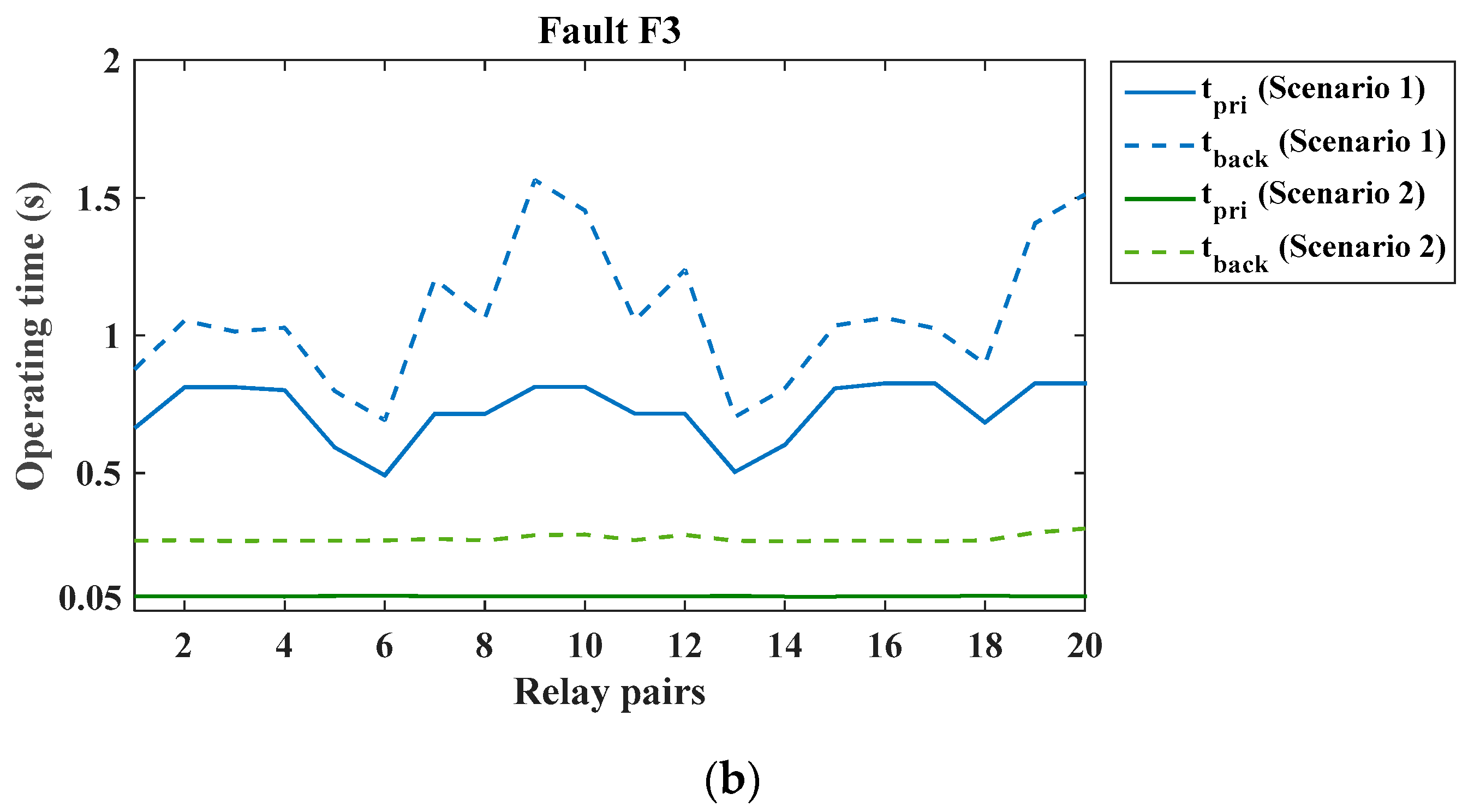
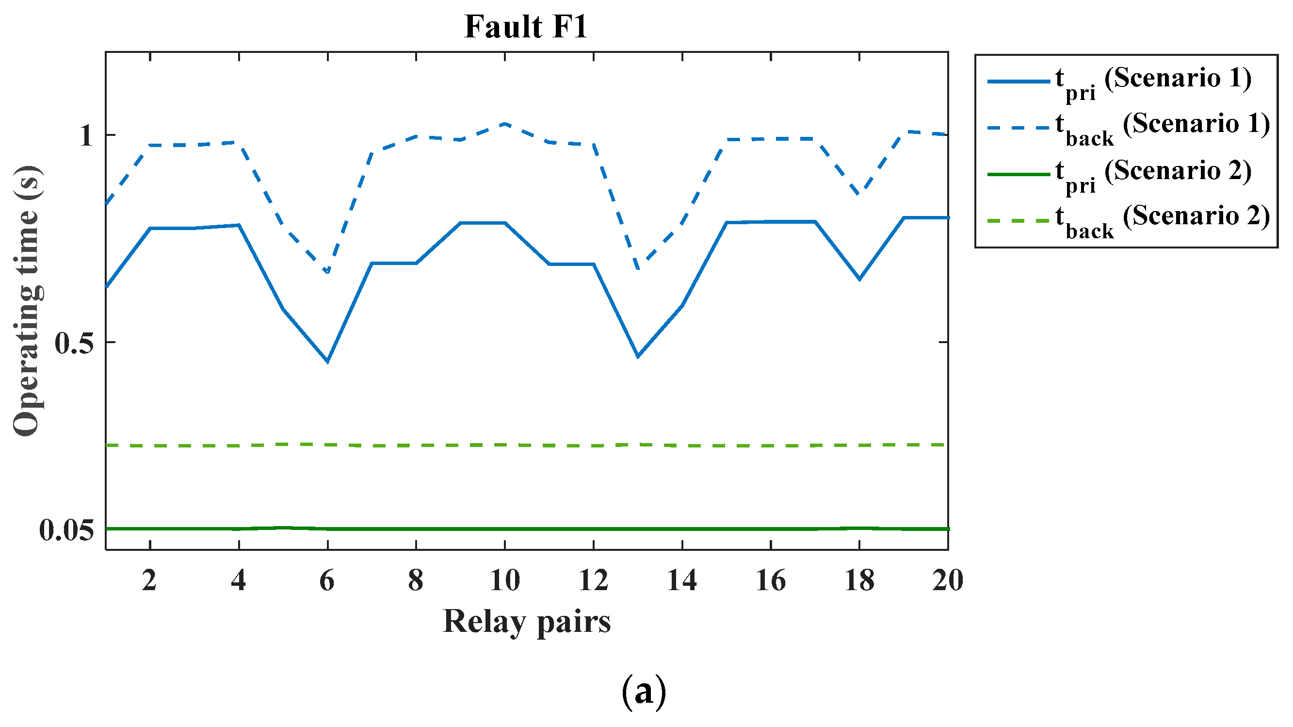
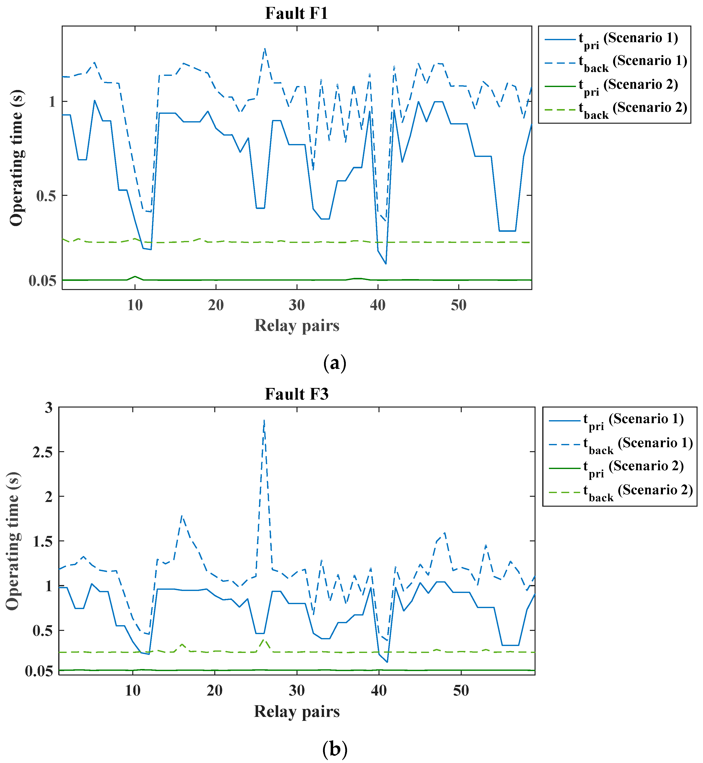
The significant difference between Scenarios 1 and 2 can also be visually observed in Figure 5, which illustrates the primary and backup relay operating times for DOCR–DOCR coordination at the F1 and F3 fault locations. For Scenario 2, all primary relay operating times at the F1 and F3 fault locations are seen to lie on the minimum operating time limit of 0.05 s. Similarly, when the backup relay operating times are examined, it is observed that the high, widely varying backup operating times observed for different relay pairs in Scenario 1 are significantly lower and closer in Scenario 2.

These results indicate that, within the scope of Scenario 2, the flexibility provided by the two-level DOCR characteristic used for the proposed DR–DOCR coordination enables the coordination constraints to be satisfied more easily at lower relay operating times.

Table 11. Statistical optimization results obtained via different optimization algorithms for the 8-bus test system.

Algorithm	Scenario 1					Scenario 2
	Min	Max	Avg	Std	CPUavg	Min	Max	Avg	Std	CPUavg
APO	199.503	213.121	206.052	3.821	54.969	279.687	334.767	303.066	13.658	90.447
EEFO	134.783	145.931	140.295	2.896	63.981	26.444	31.300	28.734	1.256	111.453
EEO	132.953	158.776	147.137	6.579	53.069	33.783	135.446	44.127	21.676	83.894
GJO	146.035	165.086	157.045	5.283	51.792	26.685	31.886	29.070	1.275	91.275
GWO	143.101	159.615	151.578	4.284	52.483	26.660	31.206	28.680	1.345	92.723
HBA	141.226	153.258	147.474	3.695	55.127	25.419	29.949	27.401	1.056	88.746
JS	141.482	145.606	143.346	1.089	52.226	24.316	25.234	24.654	0.254	84.675
KOA	136.221	146.894	141.882	2.610	59.188	29.003	34.892	31.423	1.804	87.256
MSA	144.064	153.650	148.683	2.596	55.968	36.811	52.700	40.488	3.736	96.944
PSO	131.462	152.210	140.069	5.357	67.982	26.149	31.610	28.788	1.715	98.907
TLBO	130.863	141.846	136.804	2.723	57.860	25.713	36.581	28.455	2.874	86.450
RTH	130.476	144.749	137.451	4.192	81.825	23.873	28.321	25.178	1.091	143.160
ERTH	120.702	140.336	127.638	5.830	79.214	23.681	28.720	24.848	1.428	136.047

Bold values signify better results.

presents the minimum (Min), maximum (Max), average (Avg), and standard deviation (Std) values, along with the average CPU time (CPU_avg), obtained from 20 independent runs of different optimization algorithms for Scenarios 1 and 2 on the 8-bus power system.

When the results are examined, it is observed that, for Scenario 1, the ERTH algorithm provides significantly lower Min, Max, and Avg values compared with the other algorithms. On the other hand, it is observed that the Std value obtained by the ERTH algorithm is relatively high. The higher Std indicates that the ERTH algorithm does not reach near-global solutions in every run; however, the considerably low Avg value obtained via ERTH demonstrates that, compared with the other algorithms, it is more effective in exploring the promising regions of the solution space.

For Scenario 2, the JS, RTH, and ERTH algorithms exhibit closer performance. However, the ERTH algorithm yields a lower Min value, indicating that it is more effective than the other algorithms at approaching the global optimum.

On the other hand, in Scenario 2, compared to Scenario 1, the increase in the number of decision variables leads to a higher problem dimensionality, which in turn results in a greater computational burden during the iterative updating of population solutions by the algorithms. As shown in Table 11, this is reflected in the difference in average CPU time between Scenarios 1 and 2. In terms of computational cost, it is observed that the ERTH and RTH algorithms require higher computation times compared to the other algorithms. However, the lower CPU_avg value of ERTH relative to RTH indicates that the additional mechanisms incorporated into ERTH impose less computational overhead than the original stages of the RTH algorithm. At this point, it should be noted that several factors contribute to the high computational cost of the original RTH algorithm. First, the position update mechanism involves computationally expensive operations such as the Lévy flight mechanism, Gamma functions, and trigonometric calculations, which significantly increase the per-iteration cost. Second, the population mean vector is computed and utilized in all phases of the RTH algorithm—namely high soaring, low soaring, and swooping—for updating individual positions, resulting in additional computational overhead at each iteration.

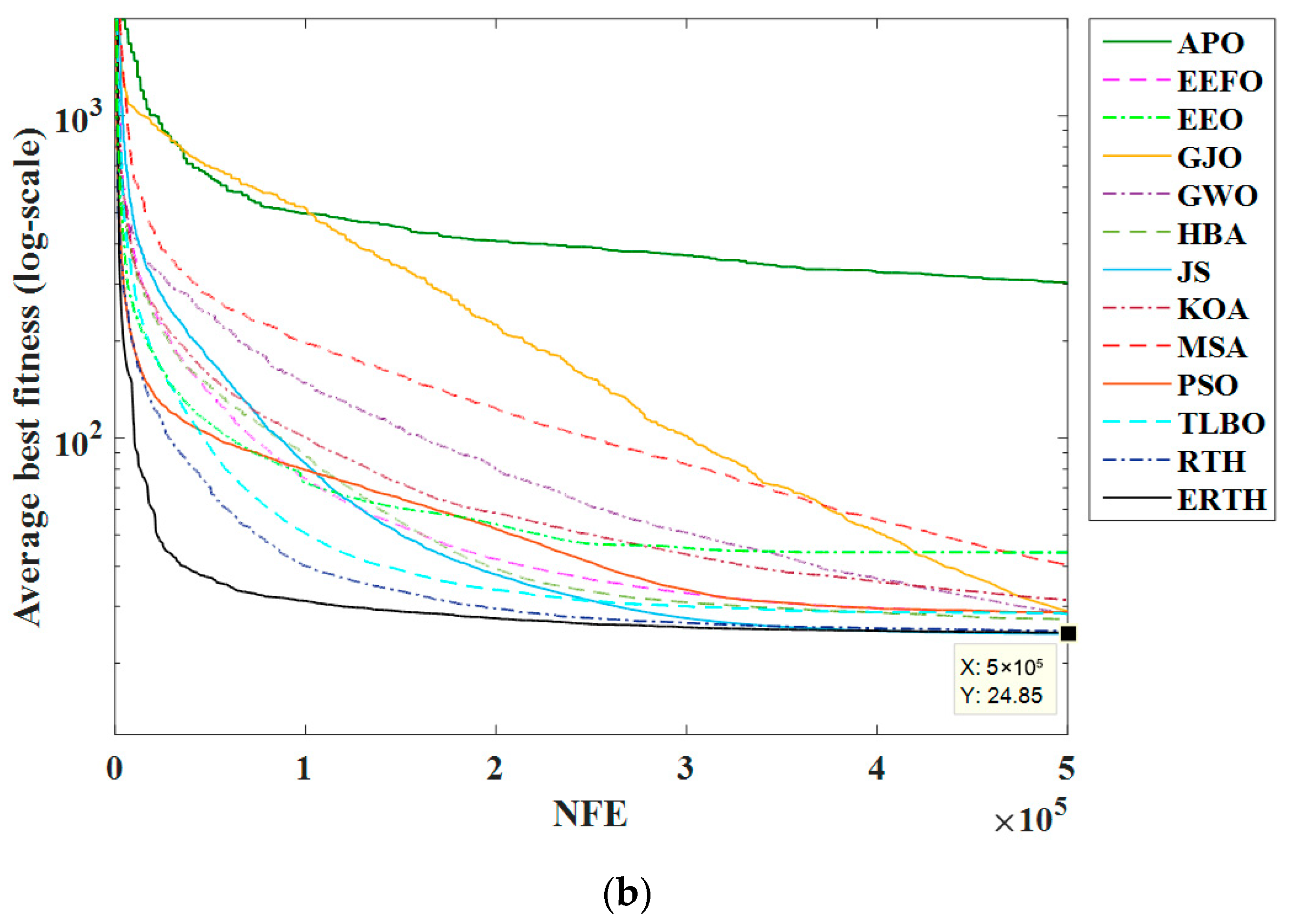
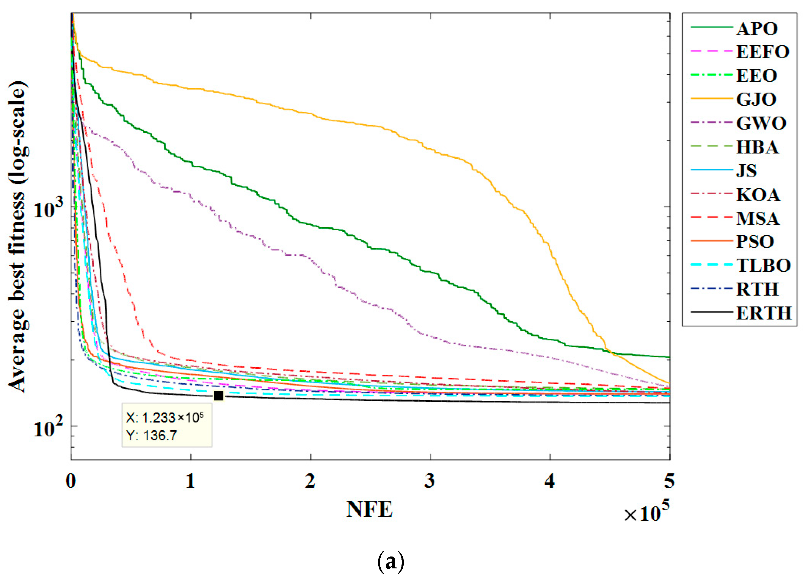
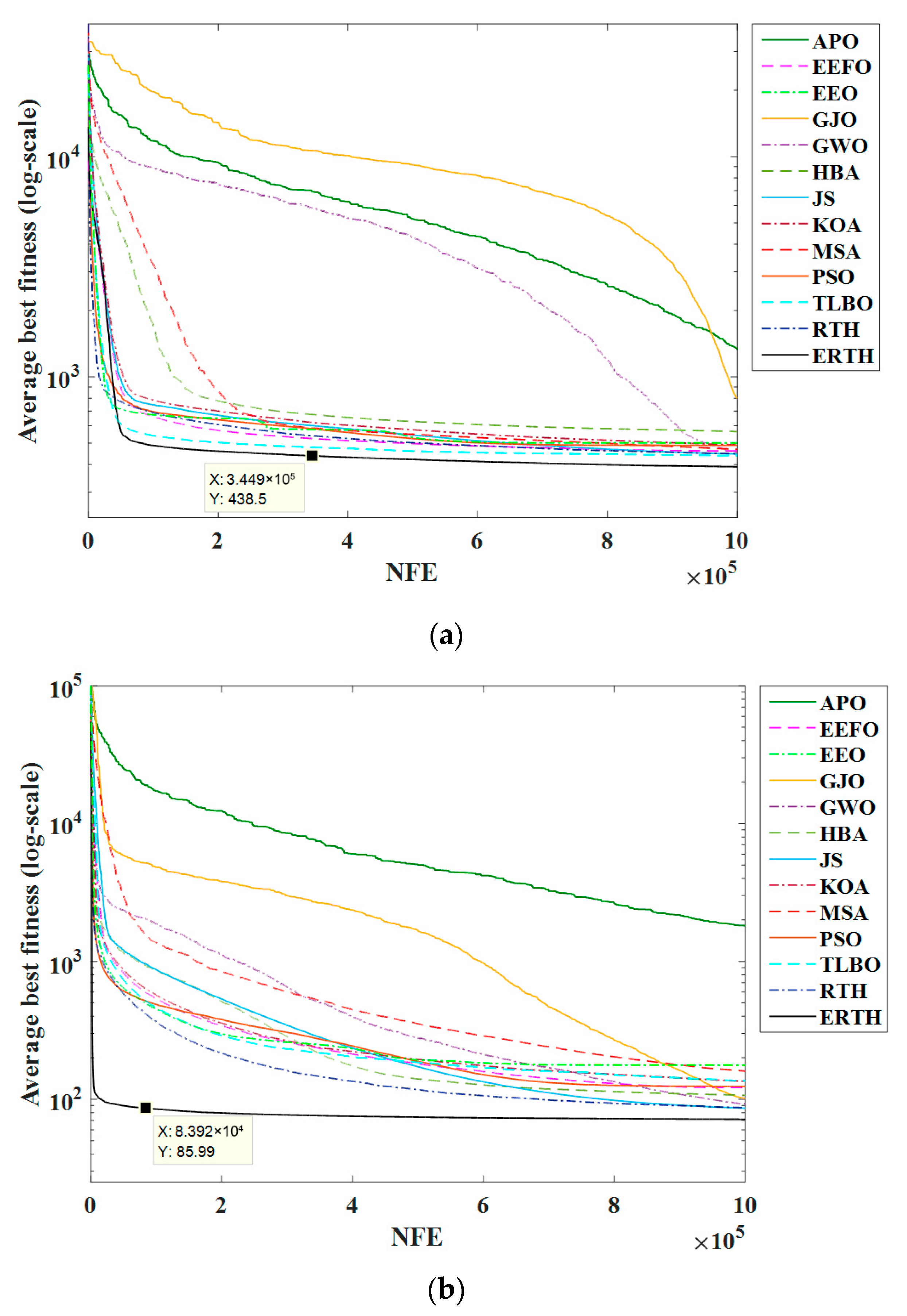
However, it should be emphasized that although both RTH and ERTH yield higher CPU_avg values compared to the other algorithms, the superior performance of ERTH compensates for this drawback. Indeed, as illustrated by the convergence curves obtained for the 8-bus power system in Figure 6, the ERTH algorithm is capable of producing effective solutions even in early iterations. Particularly for Scenario 1, it is observed that a value close to the average OF value of 136.804 s—obtained by TLBO as the second-best algorithm in this metric—is achieved by ERTH at approximately 123,300 NFE.

4.2. 30-Bus Test System

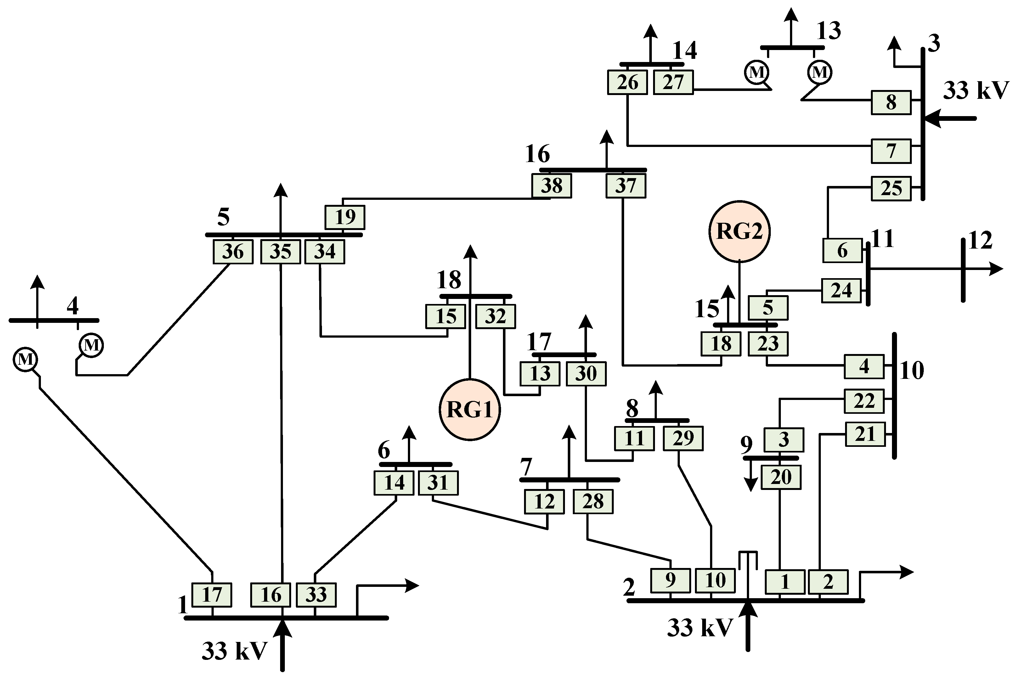
Figure 7 shows the single-line diagram of the modified 30-bus test system. The system is actually the 33 kV portion of the IEEE 30-bus system and is widely used in coordination studies [18,40]. It is assumed that renewable energy sources with a rated generation capacity of 20 MW are installed at bus nos. 15 and 18. Similar to the approach applied in the 8-bus power system, the maximum load currents flowing through the relays were obtained by considering all possible combinations of these energy sources being in service or out of service. The system includes a total of 38 relay locations and 62 relay pairs. However, for the fault locations considered in this study, the primary-backup relay pairs 1–21, 2–20, and 16–36 were excluded from the analysis because the fault current flowing through the backup relay was lower than the corresponding load current.

For the 30-bus power system, the optimal relay settings obtained using the ERTH algorithm for Scenario 1 are presented in

Table 12. Optimal relay settings obtained using the ERTH algorithm for the 30-bus system under Scenario 1.

Relay No.	${\mathbf{TDS}}_{\mathit{r}}$	${\mathbf{PS}}_{\mathit{r}}$	${\mathit{t}}_{\mathit{Z}\mathbf{2},\mathit{d}}$
1	0.364	486.387	1.410
2	0.358	213.376	1.254
3	0.436	202.783	1.368
4	0.448	170.285	1.297
5	0.344	54.066	0.822
6	0.153	128.233	0.812
7	0.108	190.268	0.881
8	0.113	151.663	0.503
9	0.444	268.936	1.246
10	0.432	261.329	1.340
11	0.364	248.054	1.219
12	0.436	148.086	1.216
13	0.309	216.973	1.125
14	0.404	97.106	1.185
15	0.255	189.565	1.139
16	0.322	398.777	1.260
17	0.235	175.707	1.144
18	0.566	64.218	1.268
19	0.459	91.008	1.156
20	0.120	457.253	1.162
21	0.170	220.542	1.986
22	0.243	226.534	0.825
23	0.286	160.604	1.008
24	0.505	74.906	1.347
25	0.448	191.187	1.186
26	0.050	188.295	0.901
27	0.051	112.640	1.100
28	0.271	271.918	1.309
29	0.177	286.326	1.323
30	0.264	224.186	1.103
31	0.451	142.331	1.381
32	0.311	252.160	1.231
33	0.599	104.902	1.383
34	0.442	172.892	1.277
35	0.218	400.838	1.302
36	0.171	133.679	1.198
37	0.397	62.777	1.030
38	0.362	135.228	1.611
OF(s)	376.757

, while the corresponding relay operating times and CTI values are presented in

Table 13. Relay operating times and the CTIs for the DOCR-DOCR coordination using ERTH for the 30-bus system under Scenario 1.

Primary Relay	Backup Relay	Fault F1			Fault F3
		${\mathit{t}}_{\mathit{p}\mathit{r}\mathit{i}}$	${\mathit{t}}_{\mathit{b}\mathit{a}\mathit{c}\mathit{k}}$	CTI2	${\mathit{t}}_{\mathit{p}\mathit{r}\mathit{i}}$	${\mathit{t}}_{\mathit{b}\mathit{a}\mathit{c}\mathit{k}}$	CTI4
1	28	0.928	1.131	0.203	0.976	1.183	0.206
1	29	0.928	1.130	0.201	0.976	1.226	0.249
2	28	0.690	1.144	0.454	0.743	1.238	0.495
2	29	0.690	1.150	0.461	0.743	1.326	0.583
3	1	1.007	1.207	0.200	1.022	1.232	0.211
4	2	0.896	1.101	0.205	0.934	1.173	0.238
4	3	0.896	1.099	0.203	0.934	1.157	0.223
5	4	0.528	1.095	0.567	0.550	1.167	0.617
5	37	0.528	0.851	0.323	0.550	0.900	0.350
6	5	0.365	0.622	0.257	0.373	0.633	0.260
7	6	0.218	0.418	0.200	0.249	0.479	0.230
8	6	0.212	0.413	0.201	0.231	0.457	0.226
9	20	0.937	1.138	0.200	0.961	1.295	0.334
9	21	0.937	1.138	0.201	0.961	1.245	0.284
9	29	0.937	1.140	0.202	0.961	1.291	0.330
10	20	0.891	1.202	0.311	0.947	1.791	0.844
10	21	0.891	1.184	0.293	0.947	1.534	0.586
10	28	0.891	1.165	0.274	0.947	1.388	0.441
11	10	0.948	1.150	0.202	0.962	1.167	0.205
12	9	0.857	1.061	0.204	0.890	1.110	0.220
13	11	0.820	1.022	0.201	0.841	1.049	0.208
14	12	0.822	1.022	0.200	0.850	1.062	0.212
15	13	0.729	0.935	0.206	0.761	0.978	0.218
16	14	0.806	1.007	0.201	0.853	1.069	0.216
17	14	0.432	1.016	0.584	0.466	1.104	0.638
17	35	0.432	1.285	0.853	0.466	2.857	2.392
18	4	0.897	1.097	0.200	0.936	1.180	0.244
18	24	0.897	1.099	0.201	0.936	1.150	0.214
19	15	0.770	0.970	0.200	0.799	1.075	0.276
19	16	0.770	1.078	0.308	0.799	1.153	0.354
19	17	0.770	1.078	0.308	0.799	1.182	0.383
20	22	0.428	0.632	0.204	0.467	0.673	0.206
21	3	0.375	1.117	0.743	0.407	1.287	0.880
21	23	0.375	0.789	0.414	0.407	0.820	0.413
22	2	0.577	1.092	0.514	0.586	1.125	0.539
22	23	0.577	0.782	0.204	0.586	0.787	0.201
23	24	0.648	1.092	0.444	0.672	1.118	0.446
23	37	0.648	0.848	0.200	0.672	0.890	0.218
24	25	0.949	1.149	0.200	0.980	1.199	0.220
25	-	0.979	-	-	1.013	-	-
26	8	0.206	0.410	0.204	0.230	0.452	0.222
27	7	0.135	0.362	0.227	0.142	0.386	0.245
28	31	0.956	1.188	0.232	0.982	1.212	0.230
29	30	0.676	0.887	0.211	0.717	0.934	0.217
30	32	0.816	1.017	0.201	0.828	1.033	0.204
31	33	1.000	1.203	0.203	1.033	1.240	0.206
32	34	0.891	1.091	0.200	0.915	1.117	0.201
33	35	0.997	1.201	0.204	1.041	1.493	0.452
33	36	0.997	1.200	0.202	1.041	1.591	0.551
34	16	0.881	1.081	0.200	0.925	1.168	0.243
34	17	0.881	1.082	0.202	0.925	1.205	0.279
34	38	0.881	1.081	0.200	0.925	1.176	0.251
35	15	0.708	0.958	0.250	0.756	1.006	0.249
35	17	0.708	1.106	0.398	0.756	1.457	0.701
35	38	0.708	1.067	0.359	0.756	1.102	0.345
36	15	0.311	0.970	0.659	0.331	1.062	0.732
36	16	0.311	1.097	0.786	0.331	1.273	0.942
36	38	0.311	1.078	0.767	0.331	1.154	0.824
37	19	0.705	0.909	0.204	0.730	0.944	0.214
38	18	0.879	1.080	0.201	0.909	1.109	0.200

and

Table 14. Relay operating times and the CTIs for the DR-DOCR coordination using ERTH for the 30-bus system under Scenario 1.

Primary Relay	Backup Relay	Fault F1	Fault F2	Fault F4
		CTI1	${\mathit{t}}_{\mathit{b}\mathit{a}\mathit{c}\mathit{k}}$/CTI3	${\mathit{t}}_{\mathit{p}\mathit{r}\mathit{i}}$	CTI5
1	28	0.380	1.157	1.182	0.228
1	29	0.395	1.178	1.182	0.228
2	28	0.619	1.193	1.040	0.214
2	29	0.633	1.239	1.040	0.214
3	1	0.403	1.219	1.080	0.288
4	2	0.358	1.137	1.067	0.230
4	3	0.472	1.128	1.067	0.230
5	4	0.769	1.131	0.616	0.207
5	37	0.502	0.875	0.616	0.207
6	5	0.457	0.628	0.399	0.412
7	6	0.593	0.450	0.672	0.209
8	6	0.600	0.436	0.293	0.210
9	20	0.224	1.214	1.042	0.204
9	21	1.049	1.190	1.042	0.204
9	29	0.385	1.212	1.042	0.204
10	20	0.271	1.446	1.133	0.207
10	21	1.095	1.341	1.133	0.207
10	28	0.418	1.269	1.133	0.207
11	10	0.392	1.158	1.011	0.207
12	9	0.389	1.085	1.005	0.211
13	11	0.398	1.036	0.919	0.206
14	12	0.394	1.042	0.978	0.206
15	13	0.396	0.956	0.927	0.212
16	14	0.378	1.038	1.043	0.217
17	14	0.753	1.061	0.578	0.566
17	35	0.870	1.733	0.578	0.566
18	4	0.400	1.138	1.064	0.204
18	24	0.450	1.125	1.064	0.204
19	15	0.369	1.021	0.894	0.263
19	16	0.490	1.115	0.894	0.263
19	17	0.374	1.130	0.894	0.263
20	22	0.397	0.651	0.953	0.209
21	3	0.994	1.193	0.857	1.129
21	23	0.633	0.806	0.857	1.129
22	2	0.676	1.108	0.620	0.205
22	23	0.430	0.784	0.620	0.205
23	24	0.699	1.105	0.771	0.236
23	37	0.382	0.868	0.771	0.236
24	25	0.237	1.174	1.078	0.269
25	-	-	-	1.128	-
26	8	0.297	0.429	0.692	0.209
27	7	0.746	0.374	0.174	0.926
28	31	0.425	1.200	1.105	0.203
29	30	0.427	0.909	1.044	0.279
30	32	0.415	1.025	0.873	0.230
31	33	0.384	1.221	1.170	0.211
32	34	0.385	1.104	1.006	0.225
33	35	0.305	1.332	1.183	0.200
33	36	0.201	1.369	1.183	0.200
34	16	0.379	1.125	1.074	0.203
34	17	0.263	1.142	1.074	0.203
34	38	0.730	1.127	1.074	0.203
35	15	0.431	0.982	1.091	0.211
35	17	0.437	1.244	1.091	0.211
35	38	0.904	1.084	1.091	0.211
36	15	0.828	1.017	0.406	0.792
36	16	0.949	1.179	0.406	0.792
36	38	1.300	1.117	0.406	0.792
37	19	0.451	0.927	0.829	0.201
38	18	0.389	1.094	1.044	0.567

, respectively. An examination of the results shows that there are no violations of the CTI₂ and CTI₅ constraints, which are critical for CTI violations. On the other hand, the optimal relay settings for Scenario 2 obtained using the ERTH algorithm are presented in

Table 15. Optimal relay settings using ERTH for the 30-bus system under Scenario 2.

Relay No.	${\mathbf{TDS}}_{\mathit{r},\mathbf{1}}$	${\mathbf{PS}}_{\mathit{r},\mathbf{1}}$	${\mathit{\alpha }}_{\mathit{r},\mathbf{1}}$	${\mathit{\beta }}_{\mathit{r},\mathbf{1}}$	${\mathbf{TDS}}_{\mathit{r},\mathbf{2}}$	${\mathbf{PS}}_{\mathit{r},\mathbf{2}}$	${\mathit{\alpha }}_{\mathit{r},\mathbf{2}}$	${\mathit{\beta }}_{\mathit{r},\mathbf{2}}$	${\mathit{t}}_{\mathit{Z}\mathbf{2},\mathrm{d}}$	${\mathit{t}}_{\mathit{r}}^{\mathit{s}\mathit{h}}$
1	0.221	326.000	0.312	0.282	0.178	326.000	0.185	0.252	0.271	0.213
2	0.178	155.000	0.332	0.204	0.325	155.000	0.290	0.356	0.301	0.187
3	0.167	154.000	0.325	0.227	0.255	154.010	0.310	0.337	0.263	0.205
4	0.191	116.000	0.301	0.203	0.233	116.000	0.336	0.242	0.263	0.184
5	0.245	54.001	0.352	0.230	0.298	54.000	0.273	0.664	0.269	0.244
6	0.222	128.000	0.222	0.238	0.179	128.504	0.226	0.248	0.261	0.204
7	0.183	128.011	0.361	0.225	0.213	128.000	0.333	0.258	0.365	0.169
8	0.237	112.286	0.293	0.223	0.248	112.000	0.309	0.627	0.337	0.228
9	0.243	185.276	0.308	0.256	0.256	185.000	0.324	0.237	0.344	0.191
10	0.277	207.000	0.215	0.223	0.249	207.000	0.390	0.242	0.268	0.150
11	0.218	166.000	0.322	0.290	0.295	166.268	0.140	0.255	0.279	0.226
12	0.189	99.078	0.348	0.217	0.184	99.000	0.271	0.246	0.276	0.211
13	0.139	179.000	0.317	0.229	0.205	179.007	0.304	0.229	0.314	0.167
14	0.337	73.000	0.248	0.272	0.216	73.004	0.307	0.336	0.345	0.213
15	0.216	131.000	0.238	0.256	0.050	131.000	0.140	0.222	0.266	0.245
16	0.251	270.000	0.279	0.281	0.139	270.072	0.351	0.252	0.379	0.193
17	0.201	130.135	0.379	0.233	0.259	127.000	0.233	0.250	0.306	0.146
18	0.241	45.660	0.335	0.208	0.280	45.002	0.317	0.280	0.265	0.206
19	0.250	91.000	0.299	0.228	0.251	91.017	0.338	0.190	0.262	0.157
20	0.219	326.000	0.156	0.231	0.247	326.001	0.322	0.260	0.307	0.001
21	0.219	155.023	0.329	0.260	0.050	155.041	0.316	0.228	0.337	0.208
22	0.265	154.000	0.294	0.289	0.235	154.113	0.350	0.310	0.257	0.197
23	0.231	116.000	0.308	0.265	0.287	116.006	0.322	0.241	0.265	0.156
24	0.191	54.043	0.322	0.204	0.246	54.000	0.327	0.247	0.309	0.192
25	0.259	128.003	0.255	0.240	0.201	128.001	0.310	0.230	0.257	0.189
26	0.235	128.001	0.251	0.378	0.250	128.000	0.381	0.404	0.348	0.198
27	0.238	112.393	0.151	0.212	0.282	112.000	0.339	0.214	0.351	0.352
28	0.265	185.000	0.287	0.393	0.212	185.095	0.276	0.312	0.371	0.184
29	0.230	207.051	0.145	0.242	0.081	207.007	0.283	0.234	0.362	0.192
30	0.249	166.098	0.153	0.225	0.298	166.016	0.333	0.305	0.382	0.156
31	0.250	99.557	0.236	0.228	0.230	99.000	0.306	0.222	0.388	0.177
32	0.224	179.000	0.298	0.308	0.147	179.021	0.140	0.257	0.273	0.227
33	0.247	73.000	0.315	0.213	0.254	73.039	0.395	0.370	0.269	0.217
34	0.186	131.020	0.321	0.213	0.225	131.003	0.338	0.239	0.267	0.179
35	0.239	270.000	0.327	0.375	0.229	270.000	0.372	0.256	0.367	0.088
36	0.216	127.000	0.317	0.229	0.052	127.067	0.140	0.253	0.272	0.226
37	0.203	45.000	0.355	0.216	0.247	45.021	0.310	0.283	0.269	0.205
38	0.176	91.001	0.311	0.231	0.123	91.000	0.279	0.229	0.393	0.214
OF(s)	70.742

, and the relay operating times together with the values of six CTI constraints (CTI₁–CTI₆) at five different fault locations (F1–F5) are provided in

Table 16. Relay operating times and the CTIs for the DOCR-DOCR coordination using ERTH for the 30-bus system under Scenario 2.

Primary Relay	Backup Relay	Fault F1			Fault F3
		${\mathit{t}}_{\mathit{p}\mathit{r}\mathit{i}}$	${\mathit{t}}_{\mathit{b}\mathit{a}\mathit{c}\mathit{k}}$	CTI2	${\mathit{t}}_{\mathit{p}\mathit{r}\mathit{i}}$	${\mathit{t}}_{\mathit{b}\mathit{a}\mathit{c}\mathit{k}}$	CTI4
1	28	0.050	0.250	0.200	0.053	0.253	0.200
1	29	0.050	0.250	0.200	0.053	0.254	0.201
2	28	0.050	0.251	0.201	0.055	0.257	0.202
2	29	0.050	0.251	0.201	0.055	0.259	0.204
3	1	0.050	0.251	0.200	0.051	0.252	0.200
4	2	0.050	0.251	0.201	0.053	0.256	0.204
4	3	0.050	0.250	0.200	0.053	0.254	0.201
5	4	0.050	0.252	0.202	0.053	0.257	0.204
5	37	0.050	0.251	0.201	0.053	0.254	0.201
6	5	0.051	0.252	0.201	0.052	0.252	0.200
7	6	0.050	0.251	0.201	0.059	0.260	0.201
8	6	0.050	0.251	0.200	0.056	0.257	0.201
9	20	0.050	0.250	0.200	0.052	0.276	0.224
9	21	0.050	0.250	0.200	0.052	0.253	0.202
9	29	0.050	0.251	0.201	0.052	0.257	0.206
10	20	0.050	0.261	0.211	0.054	0.345	0.290
10	21	0.050	0.252	0.201	0.054	0.262	0.208
10	28	0.050	0.252	0.202	0.054	0.266	0.211
11	10	0.050	0.250	0.200	0.051	0.252	0.201
12	9	0.050	0.263	0.213	0.053	0.267	0.214
13	11	0.050	0.265	0.215	0.052	0.267	0.215
14	12	0.050	0.251	0.201	0.052	0.253	0.200
15	13	0.050	0.250	0.200	0.053	0.255	0.202
16	14	0.050	0.251	0.201	0.054	0.254	0.200
17	14	0.050	0.251	0.201	0.055	0.256	0.200
17	35	0.050	0.260	0.210	0.055	0.407	0.351
18	4	0.051	0.252	0.201	0.054	0.258	0.204
18	24	0.051	0.252	0.201	0.054	0.256	0.202
19	15	0.050	0.256	0.206	0.053	0.258	0.205
19	16	0.050	0.250	0.200	0.053	0.254	0.202
19	17	0.050	0.250	0.200	0.053	0.260	0.207
20	22	0.050	0.251	0.201	0.055	0.255	0.201
21	3	0.050	0.251	0.201	0.056	0.261	0.205
21	23	0.050	0.252	0.202	0.056	0.256	0.200
22	2	0.050	0.250	0.200	0.051	0.253	0.202
22	23	0.050	0.251	0.201	0.051	0.251	0.200
23	24	0.050	0.252	0.201	0.053	0.253	0.200
23	37	0.050	0.250	0.200	0.053	0.254	0.201
24	25	0.050	0.250	0.200	0.052	0.253	0.201
25	-	0.050	-	-	0.052	-	-
26	8	0.050	0.254	0.204	0.057	0.258	0.201
27	7	0.050	0.250	0.200	0.053	0.256	0.203
28	31	0.051	0.253	0.202	0.053	0.255	0.203
29	30	0.050	0.252	0.202	0.053	0.258	0.204
30	32	0.050	0.251	0.201	0.051	0.251	0.200
31	33	0.050	0.251	0.201	0.052	0.252	0.200
32	34	0.051	0.251	0.200	0.052	0.253	0.200
33	35	0.050	0.250	0.200	0.053	0.285	0.232
33	36	0.050	0.250	0.200	0.053	0.258	0.205
34	16	0.050	0.250	0.200	0.053	0.255	0.202
34	17	0.050	0.251	0.201	0.053	0.262	0.209
34	38	0.050	0.254	0.204	0.053	0.258	0.205
35	15	0.050	0.256	0.206	0.054	0.257	0.202
35	17	0.050	0.253	0.203	0.054	0.285	0.231
35	38	0.050	0.253	0.203	0.054	0.255	0.200
36	15	0.050	0.256	0.206	0.055	0.257	0.203
36	16	0.050	0.251	0.201	0.055	0.261	0.207
36	38	0.050	0.254	0.204	0.055	0.257	0.202
37	19	0.050	0.250	0.200	0.053	0.255	0.202
38	18	0.050	0.251	0.200	0.052	0.252	0.200

and

Table 17. Relay operating times and the CTIs for the DR-DOCR coordination using ERTH for the 30-bus system under Scenario 2.

Primary Relay	Backup Relay	Fault F1	Fault F2	Fault F4		Fault F5
		CTI1	${\mathit{t}}_{\mathit{b}\mathit{a}\mathit{c}\mathit{k}}$/CTI3	${\mathit{t}}_{\mathit{p}\mathit{r}\mathit{i}}$	CTI5	${\mathit{t}}_{\mathit{p}\mathit{r}\mathit{i}}$	CTI6
1	28	0.321	0.252	0.067	0.204	0.052	0.318
1	29	0.312	0.252	0.067	0.204	0.052	0.310
2	28	0.320	0.254	0.082	0.219	0.054	0.317
2	29	0.312	0.255	0.082	0.219	0.054	0.309
3	1	0.221	0.251	0.055	0.208	0.051	0.220
4	2	0.251	0.254	0.062	0.201	0.052	0.249
4	3	0.213	0.252	0.062	0.201	0.052	0.211
5	4	0.213	0.255	0.063	0.206	0.052	0.210
5	37	0.219	0.253	0.063	0.206	0.052	0.217
6	5	0.218	0.252	0.057	0.204	0.052	0.217
7	6	0.211	0.256	0.164	0.201	0.057	0.204
8	6	0.211	0.254	0.075	0.262	0.055	0.206
9	20	0.257	0.263	0.057	0.286	0.051	0.256
9	21	0.287	0.252	0.057	0.286	0.051	0.286
9	29	0.312	0.254	0.057	0.286	0.051	0.311
10	20	0.257	0.299	0.068	0.201	0.053	0.254
10	21	0.287	0.256	0.068	0.201	0.053	0.284
10	28	0.320	0.259	0.068	0.201	0.053	0.317
11	10	0.218	0.251	0.055	0.225	0.051	0.217
12	9	0.293	0.265	0.061	0.215	0.052	0.291
13	11	0.229	0.266	0.057	0.257	0.051	0.228
14	12	0.226	0.252	0.063	0.282	0.052	0.224
15	13	0.264	0.252	0.066	0.201	0.052	0.262
16	14	0.295	0.252	0.069	0.310	0.053	0.292
17	14	0.295	0.254	0.073	0.233	0.054	0.291
17	35	0.317	0.310	0.073	0.233	0.054	0.313
18	4	0.212	0.255	0.064	0.201	0.053	0.210
18	24	0.258	0.254	0.064	0.201	0.053	0.256
19	15	0.216	0.257	0.062	0.200	0.052	0.214
19	16	0.329	0.252	0.062	0.200	0.052	0.327
19	17	0.256	0.255	0.062	0.200	0.052	0.254
20	22	0.207	0.253	0.106	0.201	0.053	0.203
21	3	0.213	0.256	0.128	0.209	0.054	0.209
21	23	0.215	0.254	0.128	0.209	0.054	0.211
22	2	0.251	0.252	0.055	0.202	0.051	0.250
22	23	0.215	0.251	0.055	0.202	0.051	0.214
23	24	0.258	0.252	0.063	0.202	0.052	0.257
23	37	0.219	0.252	0.063	0.202	0.052	0.217
24	25	0.207	0.252	0.059	0.250	0.052	0.206
25	-	-	-	0.060	-	0.052	-
26	8	0.287	0.256	0.147	0.200	0.055	0.283
27	7	0.315	0.253	0.069	0.282	0.052	0.312
28	31	0.337	0.254	0.061	0.310	0.052	0.336
29	30	0.332	0.254	0.077	0.285	0.052	0.329
30	32	0.223	0.251	0.054	0.328	0.051	0.222
31	33	0.219	0.252	0.061	0.327	0.052	0.218
32	34	0.216	0.252	0.059	0.214	0.052	0.215
33	35	0.317	0.266	0.063	0.207	0.052	0.315
33	36	0.222	0.254	0.063	0.207	0.052	0.220
34	16	0.329	0.253	0.064	0.202	0.053	0.326
34	17	0.256	0.256	0.064	0.202	0.053	0.254
34	38	0.343	0.256	0.064	0.202	0.053	0.341
35	15	0.216	0.257	0.083	0.285	0.053	0.213
35	17	0.256	0.266	0.083	0.285	0.053	0.253
35	38	0.343	0.254	0.083	0.285	0.053	0.340
36	15	0.216	0.257	0.072	0.200	0.053	0.213
36	16	0.329	0.256	0.072	0.200	0.053	0.325
36	38	0.343	0.256	0.072	0.200	0.053	0.340
37	19	0.212	0.253	0.062	0.207	0.052	0.210
38	18	0.215	0.251	0.061	0.332	0.052	0.213

. It is observed that the OF value, which was obtained as 376.757 s in Scenario 1, decreases to 70.742 s in Scenario 2, corresponding to an approximately 81% reduction, close to the decrease obtained for the 8-bus system. This significant difference between Scenario 1 and Scenario 2 is also evident in the relay operating times shown in Figure 8.

According to the statistical optimization results obtained for the 30-bus power system presented in

Table 18. Statistical optimization results obtained via different optimization algorithms for the 30-bus test system.

Algorithm	Scenario 1					Scenario 2
	Min	Max	Avg	Std	CPUavg	Min	Max	Avg	Std	CPUavg
APO	943.434	1700.943	1333.431	205.211	274.699	1473.968	2143.999	1819.670	219.482	450.962
EEFO	437.463	486.158	461.496	12.115	290.664	99.486	136.333	121.701	10.409	547.713
EEO	469.560	582.868	501.079	27.936	227.565	147.609	320.279	176.306	36.653	425.698
GJO	418.824	1853.008	800.730	396.156	243.925	94.074	110.443	101.523	3.845	448.010
GWO	431.961	473.260	453.974	11.170	239.154	88.113	99.927	92.748	3.264	443.689
HBA	479.626	631.188	564.356	37.344	260.922	90.388	128.924	106.697	11.028	436.148
JS	437.237	455.872	446.169	5.661	244.232	76.933	97.127	86.060	5.833	397.169
KOA	449.542	542.721	490.775	26.891	250.104	122.653	147.255	134.887	6.810	386.413
MSA	424.448	512.654	468.811	28.210	265.697	141.543	186.881	159.965	11.665	442.487
PSO	444.525	520.711	488.471	21.541	273.926	103.642	135.546	123.853	7.967	409.818
TLBO	415.885	468.950	438.641	15.491	259.015	108.132	214.442	135.787	25.548	382.835
RTH	419.725	506.170	448.016	22.897	352.284	78.461	98.442	86.530	4.741	917.970
ERTH	376.757	403.537	390.744	8.742	338.701	70.742	72.812	71.521	0.508	861.348

Bold values signify better results.

, the superiority of the ERTH algorithm over the competing algorithms becomes much more prominent compared to the results obtained for the 8-bus power system. It is observed that the ERTH algorithm performs as the best method in Min, Max, and Avg values. This effective performance can also be observed in the convergence curves obtained for the 30-bus system, as shown in Figure 9.

On the other hand, an examination of the CPU_avg values presented in Table 18 indicates that the RTH and ERTH algorithms are computationally expensive compared to the other algorithms. However, as illustrated in Figure 9, for Scenarios 1 and 2, values close to the second-best average OF values—obtained by TLBO and JS at the end of the optimization—are achieved by ERTH at approximately 344,900 and 83,920 NFE, respectively. This indicates that although the ERTH algorithm results in a high computational cost by the end of the optimization process, it is capable of attaining competitive solutions at much earlier stages. In other words, even before reaching half of the total computational effort, ERTH can produce better results compared to the other algorithms.

All these results indicate that the ERTH algorithm is a highly effective method for solving the coordination problem in both small- and large-scale power systems, with particularly strong performance in large-scale power systems.

4.3. Performance Evaluation Under Consideration of Multiple Fault Types

Three-phase short-circuit (3-L) faults are considered the most severe type of fault in power systems due to the high magnitude of the resulting fault currents and their associated impacts. Therefore, fast and reliable protection measures are required against such faults. Accordingly, in the majority of relay coordination studies, fault currents corresponding to three-phase short circuits are typically employed. However, in practical power systems, in addition to three-phase faults, line-to-line (L-L) and single line-to-ground (L-G) faults may also occur, and their occurrence probabilities are, in fact, higher than those of three-phase faults.

In this context, to evaluate the performance of the proposed method under different fault conditions, the objective function values associated with line-to-line and single line-to-ground faults, in addition to the three-phase short-circuit fault, are incorporated into the problem formulation. Accordingly, the modified objective function considered in this study is defined as the summation of relay operating times obtained for these three fault types based on their respective fault currents, i.e., ${\mathrm{OF}}_{\mathrm{TOT}}$ = ${\mathrm{OF}}_{3\text{-}\mathrm{L}}$ + ${\mathrm{OF}}_{\mathrm{L}\text{-}\mathrm{L}}$ + ${\mathrm{OF}}_{\mathrm{L}\text{-}\mathrm{G}}$. Consequently, the number of coordination time interval (CTI) constraints is also tripled. Within this framework, a single relay setting group must satisfy all CTI constraints for all fault types, which significantly increases the complexity of the optimization problem.

The simulations are carried out on the 30-bus power system. The TLBO and JS algorithms—which provide the second-best results for Scenarios 1 and 2 in Table 18, respectively—are considered for comparison purposes. The minimum objective function values obtained from 20 independent runs are presented in

Table 19. Optimization results obtained for multiple fault type consideration.

Scenario	Algorithm	${\mathbf{OF}}_{\mathbf{TOT}}$	${\mathbf{OF}}_{\mathbf{3}\mathbf{\text{-}}\mathbf{L}}$	${\mathbf{OF}}_{\mathbf{L}\mathbf{\text{-}}\mathbf{L}}$	${\mathbf{OF}}_{\mathbf{L}\mathbf{\text{-}}\mathbf{G}}$
Scenario 1	TLBO	1411.616	455.046	469.938	486.632
	ERTH	1223.166	382.036	408.554	432.576
Scenario 2	JS	341.716	117.129	109.894	114.693
	ERTH	215.526	70.656	71.799	73.071

. Consistent with the previous results, the ERTH algorithm is observed to outperform both the TLBO and JS algorithms again in this experiment.

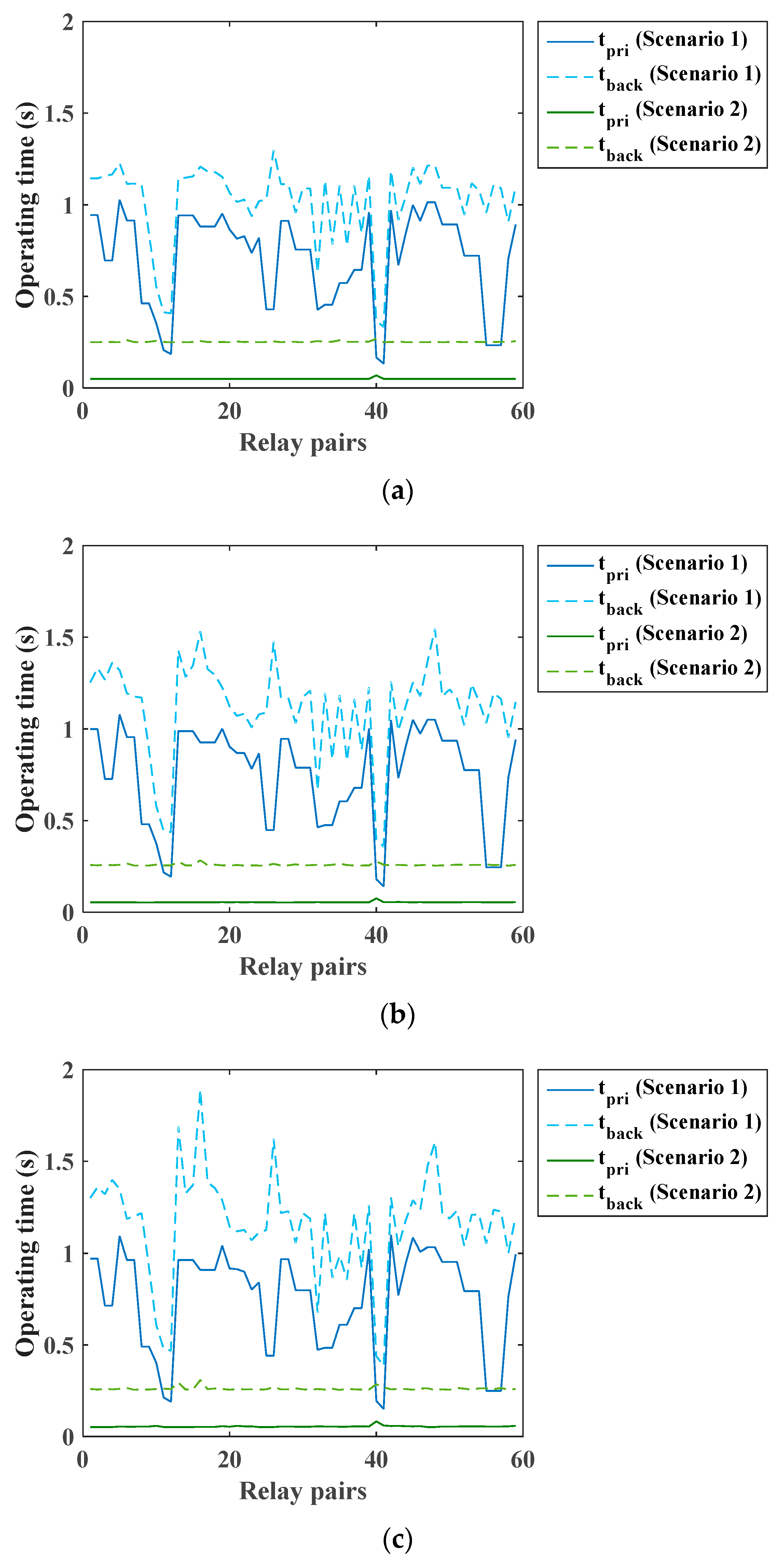
On the other hand, for Scenario 1, the objective function ($\mathrm{OF}$) value previously obtained as 376.757 s for the three-phase short-circuit fault in Table 18 is observed to increase to 382.036 s (i.e., ${\mathrm{OF}}_{3\text{-}\mathrm{L}}$) due to the increased number of constraints. In contrast, for Scenario 2, when the proposed two-level DOCR-based coordination scheme is employed with the ERTH algorithm, a result (70.656 s) very close to that reported in Table 18 (70.742 s) is achieved under this extended analysis. This clearly demonstrates the effectiveness of the proposed coordination scheme in handling increased constraint conditions. Furthermore, under line-to-line and single line-to-ground fault conditions, the fault currents flowing through backup relays decrease, which—due to the inverse-time characteristics of the relays—results in higher values of ${\mathrm{OF}}_{\mathrm{L}\text{-}\mathrm{L}}$ and ${\mathrm{OF}}_{\mathrm{L}\text{-}\mathrm{G}}$ compared to ${\mathrm{OF}}_{3\text{-}\mathrm{L}}$. However, considering the results obtained by the ERTH algorithm, this increase remains quite limited in Scenario 2 compared to Scenario 1. This effect is also evident in Figure 10, where the operating times of primary and backup relays at fault location F1 are presented.

4.4. Sensitivity Analysis for Penalty Coefficients

In optimization problems where metaheuristic methods are employed, avoiding infeasible solutions is typically achieved by incorporating a penalty term into the objective function. Accordingly, in this study, a penalty function given in Equation (4) is added to the objective function defined in Equation (1) in order to prevent CTI violations and to ensure that relay operating times do not fall below a specified minimum value. In this context, the coefficients included in the penalty function are of critical importance and are generally determined through a trial-and-error process. In the literature on optimal relay coordination, studies employing similar penalty functions assign penalty coefficients over a wide range of values, such as 100 [41], 1000 [42], and 10,000 [43] to prevent violations of CTI constraints, and 1000 [44] and 100,000 [43] to avoid violations of relay operating time constraints.

In this study, since ${\mathrm{CTI}}_{\min }$ is set to 0.2 and $t_{\min }$ is 0.05 s, the penalty coefficients associated with relay operating time violations are selected to be relatively larger. Accordingly, four different combinations of (${\delta }_1$, ${\delta }_2$), namely (100, 200), (250, 500), (500, 1000), and (2500, 5000), are considered. A sensitivity analysis is conducted using the ERTH algorithm based on 20 independent runs for the 30-bus power system. The 30-bus system is selected because the number of backup relays per primary relay is relatively high, making the satisfaction of coordination constraints more challenging.

According to the results presented in

Table 20. Sensitivity analysis results.

Parameter	Scenario 1				Scenario 2
${\delta }_1$	100	250	500	2500	100	250	500	2500
${\delta }_2$	200	500	1000	5000	200	500	1000	5000
Min OF (s)	359.480	363.366	376.757	388.498	69.455	69.852	70.742	71.308
Avg OF (s)	364.984	369.822	390.744	414.291	69.769	70.603	71.521	72.011
Avg $PenCTI$ (s)	15.181	0.624	0	0	1.391	0.046	0	0
Avg $PenT$ (s)	0	0	0	0	0.327	0.008	0	0

, it is observed that the value of the objective function increases as the penalty coefficients increase. In this context, higher penalty coefficients tend to degrade the search performance of the algorithm, whereas lower penalty values may lead to infeasible solutions. On the other hand, within the scope of Scenario 1, CTI violations are significantly higher for lower penalty coefficients compared to those in Scenario 2. These results also demonstrate that the proposed two-level DOCR-based coordination scheme in Scenario 2 is more effective in handling CTI violations. Indeed, it is observed that the penalty coefficient combination at which the algorithm achieves its best performance, without leading to infeasible solutions, is (${\delta }_1$, ${\delta }_2$) = (500, 1000).

5. Discussion and Future Research Directions

This study introduces two main innovations for optimal DR–DOCR coordination. The first is the proposal of a two-level DOCR-based DR–DOCR coordination scheme as an alternative to the conventional single-level DOCR characteristic-based coordination widely adopted in the literature, including recent studies. In conventional coordination approaches, the single-level DOCR characteristic is often insufficient to effectively handle the challenges imposed by CTI constraints, leading to relatively high operating times for both primary and backup relays. In the proposed method, the DOCR characteristic is divided into two distinct levels corresponding to primary and backup protection regions. In addition to this structural modification, the relay characteristic curve is endowed with enhanced flexibility through user-defined parameters (${\alpha }_{r,1}$, ${\alpha }_{r,2}$, ${\beta }_{r,1}, {\beta }_{r,2}$) as well as a shift parameter ($t_r^{sh}$) that controls the separation between the two levels. With these features, the proposed coordination scheme effectively mitigates CTI violations while significantly reducing relay operating times, bringing them close to the minimum allowable relay operating time ($t_{\min }$). The results obtained from the 8-bus and 30-bus test systems clearly demonstrate the effectiveness and significance of the proposed characteristic.

The second contribution of this study is the development of an enhanced version of the RTH algorithm, referred to as ERTH, for solving the coordination problem. The results indicate that the ERTH algorithm outperforms all algorithms considered, including recently applied methods for optimal DR-DOCR coordination such as GWO, EEO, and TLBO, particularly in terms of convergence toward the global optimum. Furthermore, the superior performance of ERTH in terms of both average and maximum objective function (OF) values demonstrates its robustness, consistency, and stability.

On the other hand, one of the primary drawbacks of the proposed method is that, similar to all non-standard relay characteristics, it is not directly applicable to the electromechanical relays that are still widely deployed in existing power system protection infrastructures. In this context, the proposed approach requires the use of digital relays, which may introduce additional costs. However, considering the technological advancements achieved by relay manufacturers, it is reasonable to expect that digital relays will play a much more significant role in power system protection in the near future. As also evidenced in Table 1, the use of non-standard relay characteristics has been increasingly adopted in recent studies. Moreover, with the growing penetration of renewable energy sources, power systems are increasingly exposed to challenges such as fluctuations in load currents [3], reverse fault currents under grid-connected and islanded operating modes in microgrids [11], and both short- and long-term variations in network topology [45]. Under such conditions, achieving reliable protection using conventional electromechanical relays becomes highly challenging, thereby making the adoption of digital relays essential.

Another limitation of the proposed DR–DOCR coordination approach is the significant increase in the number of decision variables compared to the conventional coordination scheme (from 3 to 10). While this increase provides enhanced flexibility in shaping the relay characteristic, it also enlarges the problem dimension and consequently increases the computational burden of the optimization process. Indeed, the results indicate that the use of the proposed relay characteristic leads to approximately a 1.5–2 times increase in computational effort. This implies that, in order to obtain optimization results within comparable time frames to conventional approaches, additional computational resources—and thus extra hardware cost—may be required. Nevertheless, it should be noted that the higher relay operating times obtained with conventional coordination approaches may impose cumulative thermal and mechanical stress on power system equipment during fault conditions, potentially leading to severe damage and significantly higher long-term costs. In this regard, the proposed method offers a more reliable and cost-effective solution from a system-level perspective.

The ERTH algorithm is observed to provide highly effective solutions for the coordination problem considered in this study. A potential shortcoming of ERTH is its computational requirement during the optimization process. However, as demonstrated by the convergence curves, ERTH is capable of reaching solution levels—often only attained by other algorithms at the end of the optimization process—at much earlier stages. This indicates that ERTH can still deliver effective performance even under lower computational time, making it a competitive and efficient optimization tool.

Under the current hardware conditions considered in this study, it is not deemed practical to employ all the investigated algorithms within a real-time relay coordination framework. However, when combined with advancements in supercomputing technologies, the strong performance demonstrated by the ERTH algorithm suggests that this integration could evolve into a powerful tool for real-time relay coordination applications.

Recent developments in relay coordination studies indicate a growing focus on addressing the challenges introduced by synchronous-based DGs, which can be based on either thermal or renewable energy sources. Due to their high fault current contributions, synchronous-based DG units can significantly alter fault current levels when they are connected to or disconnected from the system, thereby complicating protection coordination. To mitigate these effects, some studies in the literature have incorporated fault current limiters to restrict excessive fault currents [46]. Additionally, adaptive protection schemes based on assigning predefined relay setting groups in real time, in accordance with changing network topologies, have been proposed as an effective solution [47]. In contrast, the renewable energy sources considered in this study are inverter-interfaced types, which contribute relatively limited fault current. As part of future work, it is planned to extend the proposed method to scenarios involving synchronous-based renewable energy sources.

On the other hand, another research area closely related to power system protection is power system stability. Protection coordination schemes should ensure relay operating times that prevent generators from losing stability under fault conditions. Indeed, recent studies have incorporated transient stability constraints into DOCR coordination problem [48]. In this regard, future research will focus on extending the proposed method by integrating transient stability constraints into the DR–DOCR coordination framework, which, to the best of the authors’ knowledge, has not yet been addressed in the literature.

6. Conclusions

In this study, a new two-level DOCR-based DR-DOCR coordination is proposed. The proposed DR-DOCR coordination aims to achieve lower relay operating times by facilitating the avoidance of CTI violations more effectively than conventional coordination through the flexibility provided by using the two-level DOCRs. In addition, a novel variant of RTH, called ERTH, is proposed to solve the coordination problem.

The proposed method introduces two main novelties: a two-level DOCR-based coordination scheme and the use of the ERTH algorithm for optimization. It is compared with the conventional single-level DOCR coordination scheme and 12 competing optimization algorithms. Results obtained on modified 8-bus and 33 kV portions of the 30-bus test systems, including renewable energy integration, show that the proposed coordination scheme reduces relay operating times by approximately 80% and 81%, respectively, compared to the conventional method. The ERTH algorithm outperforms all other algorithms in achieving the minimum objective function, providing additional reductions of 7.5% and 9.4% compared to the second-ranked algorithms for the conventional coordination scheme in the 8-bus and 30-bus systems, respectively. Overall, a minimum reduction of 83% in relay operating times is achieved, especially for the 30-bus system, when both the proposed coordination scheme and the ERTH algorithm are employed, compared to combinations using the conventional coordination scheme and other algorithms. The method is also validated under three-phase, phase-to-phase, and single-phase-to-ground faults, demonstrating effective coordination with low relay operating times for all fault types.

The proposed scheme employs a non-standard relay characteristic, requiring digital relays. Although their higher cost may be considered a drawback, the reduced stress on power system equipment and prevention of potential damage due to shorter operating times outweigh this disadvantage. Moreover, increasing renewable energy penetration further necessitates the use of digital relays. Although the ERTH algorithm introduces a relatively high computational burden, convergence results indicate that it produces effective solutions even in early iterations.

Based on these findings, the proposed method is an effective and practical approach for DR-DOCR coordination. Future work will focus on incorporating different objective functions, additional constraints such as transient stability, and extending the method to systems with various types of renewable energy sources (e.g., synchronous and inverter-interfaced).

References

1. Korashy, A.; Kamel, S.; Jurado, F.; Eslami, M. Optimal coordination of distance relays and non-standard characteristics for directional overcurrent relays using a modified African vultures optimization algorithm. IET Gener. Transm. Distrib. 2023, 17, 2497–2522. [Google Scholar] [CrossRef] [Scilit]
2. Abdelhamid, M.; Kamel, S.; Korashy, A.; Tostado-Véliz, M.; Banakhr, F.A.; Mosaad, M.I. An adaptive protection scheme for coordination of distance and directional overcurrent relays in distribution systems based on a modified school-based optimizer. Electronics 2021, 10, 2628. [Google Scholar] [CrossRef] [Scilit]
3. Ayvaz, A. A new and effective directional overcurrent relay coordination approach for IIDG-based distribution networks using different setting groups for peak and off-peak demand periods. Electr. Power Syst. Res. 2024, 237, 111017. [Google Scholar] [CrossRef] [Scilit]
4. IEC 60255-151–2009; Measuring Relays and Protection Equipment—Part151: Functional Requirements for over/Under Current Protection. International Electrotechnical Commission: Geneva, Switzerland, 2009.
5. Damchi, Y.; Sadeh, J.; Rajabi Mashhadi, H. Optimal coordination of distance and overcurrent relays considering a non-standard tripping characteristic for distance relays. IET Gener. Transm. Distrib. 2016, 10, 1448–1457. [Google Scholar] [CrossRef] [Scilit]
6. Assouak, A.; Benabid, R. A new coordination scheme of directional overcurrent and distance protection relays considering time-voltage-current characteristics. Int. J. Electr. Power Energy Syst. 2023, 150, 109091. [Google Scholar] [CrossRef] [Scilit]
7. Rivas, A.E.L.; Pareja, L.A.G.; Abrão, T. Coordination of distance and directional overcurrent relays using an extended continuous domain ACO algorithm and an hybrid ACO algorithm. Electr. Power Syst. Res. 2019, 170, 259–272. [Google Scholar] [CrossRef] [Scilit]
8. Abdelhamid, M.; Houssein, E.H.; Mahdy, M.A.; Selim, A.; Kamel, S. An improved seagull optimization algorithm for optimal coordination of distance and directional over-current relays. Expert Syst. Appl. 2022, 200, 116931. [Google Scholar] [CrossRef] [Scilit]
9. Moravej, Z.; Ooreh, O.S. Coordination of distance and directional overcurrent relays using a new algorithm: Grey wolf optimizer. Turk. J. Electr. Eng. Comput. Sci. 2018, 26, 3130–3144. [Google Scholar] [CrossRef] [Scilit]
10. Korashy, A.; Kamel, S.; Jurado, F. Optimal coordination of directional overcurrent relays and distance relays using different optimization algorithms. Electr. Eng. 2023, 105, 2935–2947. [Google Scholar] [CrossRef] [Scilit]
11. Asl, S.A.F.; Gandomkar, M.; Nikoukar, J. Optimal protection coordination in the micro-grid including inverter-based distributed generations and energy storage system with considering grid-connected and islanded modes. Electr. Power Syst. Res. 2020, 184, 106317. [Google Scholar] [CrossRef] [Scilit]
12. Ayvaz, A. Optimal Coordination of Directional Overcurrent Relays Using an Exponential-Based Non-Standard Characteristic and the Nutcracker Optimizer. Gazi Univ. J. Sci. Part C Des. Technol. 2025, 13, 417–430. [Google Scholar] [CrossRef] [Scilit]
13. Yazdaninejadi, A.; Nazarpour, D.; Talavat, V. Coordination of mixed distance and directional overcurrent relays: Miscoordination elimination by utilizing dual characteristics for DOCR s. Int. Trans. Electr. Energ. Syst. 2019, 29, e2762. [Google Scholar] [CrossRef] [Scilit]
14. Korashy, A.; Kamel, S.; Jurado, F.; Mbasso, W.F. OptiCoord: Advancing directional overcurrent and distance relay coordination with an enhanced equilibrium optimizer. Heliyon 2024, 10, e26366. [Google Scholar] [CrossRef] [Scilit]
15. Beder, H.; Mohandes, B.; El Moursi, M.S.; Badran, E.A.; El Saadawi, M.M. A new communication-free dual setting protection coordination of microgrid. IEEE Trans. Power Del. 2020, 36, 2446–2458. [Google Scholar] [CrossRef] [Scilit]
16. Alasali, F.; El-Naily, N.; Zarour, E.; Saad, S.M. Highly sensitive and fast microgrid protection using optimal coordination scheme and nonstandard tripping characteristics. Int. J. Electr. Power Energy Syst. 2021, 128, 106756. [Google Scholar] [CrossRef] [Scilit]
17. Azari, M.; Mazlumi, K.; Ojaghi, M. Optimal directional overcurrent relay coordination in interconnected networks considering user-defined PWL characteristic curve. Arab. J. Sci. Eng. 2022, 47, 3119–3139. [Google Scholar] [CrossRef] [Scilit]
18. Fayoud, A.B.; Sharaf, H.M.; Ibrahim, D.K. Optimal coordination of DOCRs in interconnected networks using shifted user-defined two-level characteristics. Int. J. Electr. Power Energy Syst. 2022, 142, 108298. [Google Scholar] [CrossRef] [Scilit]
19. Tiwari, R.; Singh, R.K.; Choudhary, N.K. Effect of DG penetration on hybrid relay coordination using user-defined dual-setting directional overcurrent relays and distance relays. Smart Sci. 2025, 13, 45–59. [Google Scholar] [CrossRef] [Scilit]
20. He, C.; Xiao, L.; Zhang, J.; Wang, Z.; Wang, J.; Wang, L.; Zhang, L.; Wang, W.; Huang, Y.; Ouyang, D.; et al. Mechanistic insights and risk evaluation of thermal runaway in lithium-ion batteries under coupled temperature-rate conditions. Chem. Eng. J. 2026, 532, 174210. [Google Scholar] [CrossRef] [Scilit]
21. Chen, Y.; Zhu, M.; Chen, M. Comprehensive experimental research on wrapping materials influences on the thermal runaway of lithium-ion batteries. Emerg. Manag. Sci. Technol. 2025, 5, e007. [Google Scholar] [CrossRef] [Scilit]
22. Rajaei, N. Fault Current Management in Power Systems Using Inverter-Based Distributed Generators. Ph.D. Thesis, University of Waterloo, Waterloo, ON, Canada, 2015. [Google Scholar]
23. El-Sayed, W.T.; Azzouz, M.A.; Zeineldin, H.H.; El-Saadany, E.F. A harmonic time-current-voltage directional relay for optimal protection coordination of inverter-based islanded microgrids. IEEE Trans. Smart Grid 2020, 12, 1904–1917. [Google Scholar] [CrossRef] [Scilit]
24. Ferahtia, S.; Houari, A.; Rezk, H.; Djerioui, A.; Machmoum, M.; Motahhir, S.; Ait-Ahmed, M. Red-tailed hawk algorithm for numerical optimization and real-world problems. Sci. Rep. 2023, 13, 12950. [Google Scholar] [CrossRef] [Scilit] [PubMed]
25. Alshahrani, H.J.; Hassan, A.Q.; Almalki, N.S.; Alnfiai, M.M.; Salama, A.S.; Hamza, M.A. Applied linguistics with red-tailed hawk optimizer-based ensemble learning strategy in natural language processing. IEEE Access 2023, 11, 132448–132456. [Google Scholar] [CrossRef] [Scilit]
26. Almousa, M.T.; Gomaa, M.R.; Ghasemi, M.; Louzazni, M. Single-Sensor Global MPPT for PV System Interconnected with DC Link Using Recent Red-Tailed Hawk Algorithm. Energies 2024, 17, 3391. [Google Scholar] [CrossRef] [Scilit]
27. Wang, W.C.; Tian, W.C.; Xu, D.M.; Zang, H.F. Arctic puffin optimization: A bio-inspired metaheuristic algorithm for solving engineering design optimization. Adv. Eng. Softw. 2024, 195, 103694. [Google Scholar] [CrossRef] [Scilit]
28. Zhao, W.; Wang, L.; Zhang, Z.; Fan, H.; Zhang, J.; Mirjalili, S.; Khodadadi, N.; Cao, Q. Electric eel foraging optimization: A new bio-inspired optimizer for engineering applications. Expert Syst. Appl. 2024, 238, 122200. [Google Scholar] [CrossRef] [Scilit]
29. Chopra, N.; Ansari, M.M. Golden jackal optimization: A novel nature-inspired optimizer for engineering applications. Expert Syst. Appl. 2022, 198, 116924. [Google Scholar] [CrossRef] [Scilit]
30. Mirjalili, S.; Mirjalili, S.M.; Lewis, A. Grey wolf optimizer. Adv. Eng. Softw. 2014, 69, 46–61. [Google Scholar] [CrossRef] [Scilit]
31. Hashim, F.A.; Houssein, E.H.; Hussain, K.; Mabrouk, M.S.; Al-Atabany, W. Honey Badger Algorithm: New metaheuristic algorithm for solving optimization problems. Math. Comput. Simul. 2022, 192, 84–110. [Google Scholar] [CrossRef] [Scilit]
32. Chou, J.S.; Truong, D.N. A novel metaheuristic optimizer inspired by behavior of jellyfish in ocean. Appl. Math. Comput. 2021, 389, 125535. [Google Scholar] [CrossRef] [Scilit]
33. Abdel-Basset, M.; Mohamed, R.; Azeem, S.A.A.; Jameel, M.; Abouhawwash, M. Kepler optimization algorithm: A new metaheuristic algorithm inspired by Kepler’s laws of planetary motion. Knowl. Based. Syst. 2023, 268, 110454. [Google Scholar] [CrossRef] [Scilit]
34. Abdel-Basset, M.; Mohamed, R.; Zidan, M.; Jameel, M.; Abouhawwash, M. Mantis Search Algorithm: A novel bio-inspired algorithm for global optimization and engineering design problems. Comput. Methods Appl. Mech. Eng. 2023, 415, 116200. [Google Scholar] [CrossRef] [Scilit]
35. Kennedy, J.; Eberhart, R. Particle swarm optimization. IEEE International Conference on Neural Networks, Perth, WA, Australia, 27 November 1995. [Google Scholar]
36. Rao, R.V.; Savsani, V.J.; Vakharia, D.P. Teaching–learning-based optimization: A novel method for constrained mechanical design optimization problems. Comput. Aided Des. 2011, 43, 303–315. [Google Scholar] [CrossRef] [Scilit]
37. Arteaga, G.; Candelo-Becerra, J.E.; Montano, J.; Revelo-Fuelagán, J.; Hoyos, F.E. Edge Computing Architecture for Optimal Settings of Inverse Time Overcurrent Relays in Mesh Microgrids. Electricity 2026, 7, 14. [Google Scholar] [CrossRef] [Scilit]
38. Shen, Z.; Sun, Z.; Bi, Y.; Sun, Z. A Chaos-Initiated and Adaptive Multi-Guide Control-Based Crayfish Optimization Algorithm for Image Analysis. Symmetry 2025, 17, 1940. [Google Scholar] [CrossRef] [Scilit]
39. Al-Bhadely, F.; İnan, A. Improving directional overcurrent relay coordination in distribution networks for optimal operation using hybrid genetic algorithm with sequential quadratic programming. Energies 2023, 16, 7031. [Google Scholar] [CrossRef] [Scilit]
40. Korashy, A.; Kamel, S.; Jurado, F.; Youssef, A.R. Hybrid whale optimization algorithm and grey wolf optimizer algorithm for optimal coordination of direction overcurrent relays. Electr. Power Compon. Syst. 2019, 47, 644–658. [Google Scholar] [CrossRef] [Scilit]
41. Sampaio, F.C.; Tofoli, F.L.; Melo, L.S.; Barroso, G.C.; Sampaio, R.F.; Leão, R.P.S. Adaptive fuzzy directional bat algorithm for the optimal coordination of protection systems based on directional overcurrent relays. Electr. Power Syst. Res. 2022, 211, 108619. [Google Scholar] [CrossRef] [Scilit]
42. Moirangthem, J.; K.R., K.; Dash, S.S.; Ramaswami, R. Adaptive differential evolution algorithm for solving non-linear coordination problem of directional overcurrent relays. IET Gener. Transm. Distrib. 2013, 7, 329–336. [Google Scholar] [CrossRef] [Scilit]
43. El-Fergany, A.A.; Hasanien, H.M. Water cycle algorithm for optimal overcurrent relays coordination in electric power systems. Soft Comput. 2019, 23, 12761–12778. [Google Scholar] [CrossRef] [Scilit]
44. Draz, A.; Elkholy, M.M.; El-Fergany, A.A. Slime mould algorithm constrained by the relay operating time for optimal coordination of directional overcurrent relays using multiple standardized tripping curves. Neural Comput. Appl. 2021, 33, 11875–11887. [Google Scholar] [CrossRef] [Scilit]
45. Sati, T.E.; Azzouz, M.A. Optimal protection coordination for inverter dominated islanded microgrids considering N-1 contingency. IEEE Trans. Power Del. 2021, 37, 2256–2267. [Google Scholar] [CrossRef] [Scilit]
46. Mohamedshareef, R.; Abapour, M.; Hosseini, S.H.; Seyedi, H. Optimal overcurrent relay coordination: Balancing costs, time performance and generator placement in fault current limiter optimization. IET Gener. Transm. Distrib. 2024, 18, 1431–1448. [Google Scholar] [CrossRef] [Scilit]
47. Karimkhan-Zand, H.; Mazlumi, K.; Hashemi-Dezaki, H.; Abdali, A.; Vasquez, J.C. A creative approach for the protection coordination of microgrids considering parallel events via the pyramidal grouping technique. Sci. Rep. 2025, 15, 45520. [Google Scholar] [CrossRef] [Scilit] [PubMed]
48. Poursaeed, A.H.; Namdari, F. Online transient stability assessment implementing the weighted least-square support vector machine with the consideration of protection relays. Prot. Control Mod. Power Syst. 2024, 10, 1–17. [Google Scholar] [CrossRef] [Scilit]
Figure 1. The conventional coordination of DRs and DOCRs.
Applsci 16 03961 g001
Figure 2. The proposed coordination of DRs and DOCRs.
Applsci 16 03961 g002
Figure 3. Flowchart of the ERTH algorithm.
Applsci 16 03961 g003
Figure 4. Single-line diagram of the modified 8-bus test system.
Applsci 16 03961 g004
Figure 5. Relay operating times obtained using ERTH for the 8-bus system under different scenarios for DOCR-DOCR coordination at fault locations (a) F1 and (b) F3.
Applsci 16 03961 g005aApplsci 16 03961 g005b
Figure 6. Convergence curves obtained via different algorithms for the 8-bus system under (a) Scenario 1 and (b) Scenario 2.
Applsci 16 03961 g006aApplsci 16 03961 g006b
Figure 7. Single-line diagram of the modified 30-bus test system.
Applsci 16 03961 g007
Figure 8. Relay operating times obtained using ERTH for the 30-bus system under different scenarios for DOCR-DOCR coordination at fault locations (a) F1 and (b) F3.
Applsci 16 03961 g008
Figure 9. Convergence curves obtained via different algorithms for the 30-bus system under (a) Scenario 1 and (b) Scenario 2.
Applsci 16 03961 g009
Figure 10. Relay operating times obtained using ERTH for the 30-bus system under multiple fault type considerations at fault location F1: (a) three-phase short circuit, (b) line-to-line fault, and (c) single line-to-ground fault.
Applsci 16 03961 g010