Adaptive Traffic Signal Control Using Deep Reinforcement Learning with Noise Injection

Featured Application

An adaptive traffic signal control (ATSC) method based on advantage actor-critic (A2C), deep reinforcement learning (DRL) and noise injection (NI) that reduces waiting times by optimizing queue lengths and minimizing signal flickering in complex single intersections is presented.

Abstract

Adaptive traffic signal control (ATSC) remains a critical challenge for urban mobility. In this direction, deep reinforcement learning (DRL) has been widely investigated for ATSC, showing promising improvements in simulated environments. However, a noticeable gap remains between simulation-based results and practical implementations, due to reward formulations that do not address phase instability. Stochastic variations may trigger premature phase changes (“flickers”), affecting signal behavior and potentially limiting deployment in real scenarios. Although several works have examined delay, queues, and decentralized coordination, stability-focused variables remain comparatively less explored, particularly in single yet complex intersections. This study proposes a decentralized DRL model for ATSC with noise injection (ATSC-DRLNI) applied to a single intersection, introducing a stability-oriented reward function that integrates flickers, queue length, and advantage actor-critic (A2C) learning feedback. The model is evaluated in the Simulation of Urban MObility (SUMO) platform and compared against seven baseline methods, using real traffic data from a Mexican city for calibration and validation. Results suggest that penalizing flickers may contribute to more stable phase transitions, while reductions of up to 40% in queue length were observed in heavy-traffic scenarios. These findings indicate that incorporating stability-related variables into reward functions may help in implementing DRL-based ATSC studies.

1. Introduction

Traffic congestion is a phenomenon with a large impact around the world [1,2,3]. In the United States alone, cities such as Chicago, Boston, and New York have recorded the highest levels of congestion worldwide, with consequences for public health, induced by pollutant emissions, stress, and the time spent by drivers in traffic congestion [4,5,6,7]. Mexico City ranks fourth in traffic congestion and also faces the variety of social problems derived from this phenomenon [7,8,9]. Traffic congestion also generates significant economic losses [10], for example, in the USA, the cost of traffic congestion resulted in a loss of $74 billion nationwide [7,11]. By 2030, this phenomenon is expected to be present in many more cities due to the growth of the population and in the use of vehicles [12,13].

To reduce vehicle congestion at intersections, control of traffic lights is necessary [14,15]. However, the normal use of this technology, with fixed-time (FT) phases, cannot be very efficient because this strategy cannot respond to changing traffic situations [16]. The addition of sensors [17], allowed the design of adaptive traffic signal control (ATSC) systems [18]. During the early years of ATSC implementations, several techniques were proposed to optimize vehicular traffic. Among the most important are split cycle offset optimization technique (SCOOT) [19], self-organizing traffic lights (SOTL) [20,21,22], real-time hierarchical optimized distributed and effective system (RHODES) [23], and Sydney coordinated adaptive traffic system (SCATS) [24], which were attempts to set the timing of traffic lights more efficiently. Although these techniques were functional during the 1980s and 1990s, they are not adequate to deal with the more complex scenarios that arise with increasing vehicular traffic.

Artificial intelligence (AI) has significantly improved the performance of ATSC. Since 2015, there are more than 2500 publications related to ATCS, including mathematical modeling and AI applications [25]. Techniques such as fuzzy Logic (FL) or Genetic Algorithms (GAs) have helped to reduce traffic congestion by designing more intelligent phase-timing patterns of traffic lights [26,27]. Other new AI techniques based on machine learning (ML) are also used. In particular, a widely used subset is deep learning (DL), which has achieved important advances in the area of vehicular traffic [28]. Deep reinforcement learning (DRL) arises from the combination of DL with reinforcement learning (RL) algorithms that are used in the learning stage [29,30]. RL incorporates neural networks (NN) that, considering vehicle demand, identify characteristics of traffic behavior that are very helpful in phase-timing design [31,32,33,34].

In general, DRL techniques can be classified as centralized, where a set of traffic lights communicate and provide feedback between them for better decision making [35], and decentralized, where traffic lights act independently of each other [36]. There is also research that proposes hybrid solutions using both paradigms [37]. Due to the expected increase in the number of connected and automated vehicles (CAVs), which do have a different interaction with infrastructure or vehicular traffic, analysis of technologies to control intersections also allows the proposal of behaviors that would not be possible in regular scenarios [38].

The complexity of DRL techniques in ATSC is related to the size of the traffic network to be analyzed and the intrinsic difficulties of the algorithmic implementation of the chosen DRL model. Complexity is greater in centralized techniques because they manage several intersections simultaneously. The results obtained to date indicate that there are still pending issues, such as long execution times, convergence problems, and the large number of variables to be considered, that limit their application to real situations [31,33,39,40,41]. There are DRL techniques that have been successfully applied to a set of single intersections. However, the results reported correspond to cases where intersections and traffic conditions are similar [42,43].

Single intersection studies use variables such as queue length, waiting time, vehicle spacing, specific vehicle type, or number of vehicles approaching the intersection as reference information and work with the complexity of traffic and the given choice of variables [31]. They usually take traffic lights at the intersection as a single global agent [44]. The research in [27,45,46], shows a number of works where optimization is solved with metaheuristic-based algorithms.

Although most ATSC studies with DRL treat intersections as exclusive global agents or apply decentralized strategies to multiple intersection systems [47,48,49,50], few of them deal with the agent "anxiety" to prematurely change phase with small stochastic variations. Some studies use a decentralized approach at single intersections, modeling each traffic light as an independent agent and including the number of traffic light changes (flickers) as a specific variable [51]. This approach could allow better local coordination and traffic stability by solving the convergence problems that constrain traditional models, such as excessive changes in traffic lights that can affect traffic safety and stability [52].

It is still necessary to apply DRL models in single intersections with the intention of correcting erratic decision making and improving the stability of traffic light phases by combining flickers, waiting times, or vehicle queue sizes, as has been mentioned in [53,54,55]. Works such as [54,56,57], also confirm that these combinations have not yet been sufficiently addressed and suggest that despite the need to deal with scenarios with multiple intersections, problems with single intersections need to be solved by expanding their complexity scale. Recently, ref. [56] mentioned that the use of stable phase mechanisms using variables such as flickers has not been fully explored. In summary, the use of DRL models and algorithms in simple intersections has open problems that still need to be addressed.

In this paper, we present a novel optimization method in which we involve three elements: vehicle queue size, flickers, and advantage actor-critic (A2C) RL with noise injection (NI), using a decentralized approach that takes traffic lights as individual agents, generating communication between the different traffic lights installed at a single intersection. This type of combination of variables, agents, and communication at a single intersection has not been used before and justifies exploring its performance.

The aim of this work is to develop and evaluate a decentralized DRL framework for traffic signal control at a single intersection, incorporating a novel adaptive reward function. Although focused on a single intersection, this study is highly relevant as it provides a foundational testbed for complex traffic control strategies, demonstrates the practical benefits of integrating multiple traffic factors, and establishes principles that can be extended to multi-intersection networks.

This work differs from existing approaches by focusing on traffic signal control at a single intersection using a decentralized DRL framework, demonstrating that even in a single-node scenario, decentralization enhances local adaptability. Unlike most studies, the proposed model integrates into the reward function traffic related variables, flickers, and queue length, together with A2C learning results, providing a more comprehensive assessment of traffic dynamics. The use of A2C improves learning stability and convergence compared to traditional DRL methods. In this way, each intersection operates as an independent agent adapting to local traffic conditions. In addition, the adaptive reward function optimizes key metrics such as queue lengths and traffic balance. Overall, this methodology enables autonomous and adaptive phase optimization, reduces congestion and delays, and is scalable to multi-intersection networks while maintaining decentralized control. Finally, by grounding the model in realistic traffic data and simulations, the approach offers practical applicability and a closer approximation to real-world traffic management, setting it apart from many theoretical or simplified studies.

The main contributions of the proposed study are summarized as follows:

1.

A decentralized DRL framework with NI for single-intersection ATSC in which each traffic light operates as an independent agent that adapts to local traffic conditions.

2.

A stability-oriented reward function that integrates queue length, flickers, and A2C learning feedback in an effort to mitigate premature phase changes and support smoother convergence.

3.

A comparative evaluation against seven baseline methods performed in the Simulation of Urban MObility (SUMO) platform using real traffic data from a Mexican city for calibration and validation, suggesting improvements in queue reduction and phase stability.

4.

An effort toward narrowing the gap between simulation-based ATSC research and potential real-world applications that emphasizes the role of stability-related variables in decentralized DRL settings.

The article is organized as follows: In Section 2, a brief overview of ML and the techniques to be implemented will be given. The general problem formulation, as well as the details of the proposed model and algorithm, are presented in Section 3. Simulation details and the results of the scenarios used to verify the effectiveness of the present model are presented in Section 4. Next is Section 5, where the analysis and discussion of the highlights of this research are established. Finally, Section 6 presents the conclusions and future work on this line of research.

2. Preliminaries on Machine Learning

In this section, we will briefly explain some RL and DL preliminaries to show how the DRL and its algorithms work, their functions and categories, and to describe the actor-critic problem [29].

2.1. Artificial Neural Networks (ANNs)

Artificial neural networks (ANNs) are statistical models belonging to ML that identify data characteristics and, from them, formulate predictions for decision making [58,59]. ANNs have the following form:

$$\widehat{y}=\left(\sum _{i=1}^n{x}_i·w_i+b\right)$$

(1)

where the input estimates x are multiplied by a weight value w given for each input with a bias b added. The process is repeated for the input and outputs of each layer of the ANN.

A type of ANN named convolutional neural network (CNN) is commonly used for image-oriented processing and training, where images can be transformed into one-dimensional and grayscale vectors that are then processed pixel by pixel. Typically, CNN networks consist of several layers: fully connected layers, pooling layers, convolution layers, and nonlinear layers. The fully connected layers and the convolutional layers have tuning parameters, while the nonlinear layers and the pooling layers do not have them [60,61].

2.2. Reinforcement Learning (RL)

RL is a discrete time Markov decision process (MDP) that allows an agent to make future decisions based on current observation [62,63]. A MDP is defined by 5-tuples $\{S,A,T,R,\gamma \}$, where S represents the set of states contained in the environment; A is the set of actions that an agent can take within the environment; T is a transition function, which is the probability of movement between the states of the environment; R is the reward/penalty function that guides learning; and $\gamma \in [0,1]$ is a discount factor that impacts the weight of rewards or penalties in RL-oriented policies. This process is usually executed by trial and error and depends on the amount of information that is given to the model, its size, and the learning time.

The ultimate goal of using RL is to obtain the highest cumulative sum of agent’s learning after an extended period of training [64]. Formally defined, the overall reward $G_t$ is the maximization at time t of the sum of rewards $R_t$ evaluated at different future times, according to

$$G_t=R_{t+1}+R_{t+2}+R_{t+3}\dots +R_T,$$

(2)

where T is a previously established final time step. This type of maximization is known as reward maximization.

A variation in the RL approach consists in the use of a discount factor, in which agents weigh the rewards at future times using a discount factor.

$$G_t=\sum _{k=0}^{\infty }{\gamma }^k{R}_{t+k+1}.$$

(3)

There are other forms oriented to maximize the cumulative reward by maximizing the actual value of the reward $R\left(t\right)$ for any given time t.

2.3. Q-Learning (DQN)

To obtain the optimal reward, Q-Learning is used that is based on evaluating the different agent’s actions using $\epsilon$-greedy, a learning policy based on the exploration of the agent possible actions. At initial times, random actions are explored as a trial-and-error learning activity [65,66]; as time progresses, the best-performing rewards are exploited, and the best actions are selected. A $\epsilon$-greedy algorithm is easy to understand and provides greater accuracy in learning, given a training time. The updating function $Q{L}_t$ is of form

$$Q{L}_t(s,a)=Q{L}_{t-1}(s,a)+\alpha \left[R_t+\gamma \underset{\forall a^{\prime }}{max}\{Q{L}_t(s,a^{\prime })-Q{L}_{t-1}(s,a)\}\right],$$

(4)

where a are the actions, $\alpha \in [0,1]$ defines the learning rate or step size; if $\alpha =0$, the agent will never learn from the new actions; conversely, if $\alpha \to 1$ the agent will favor recent information, as the value of $Q{L}_t(s,a)$ is modified more quickly. The innovation term depends on the reward $R_t$ and the choice of the action a that maximizes the growth of $Q{L}_t(s,a)$, weighted by $\gamma \in [0,1]$, a discount factor, which in Q-Learning, determines the significance of the upcoming actions. If $\gamma$ is set to 0, the agent discards future rewards entirely and only considers current rewards; on the other hand, if $\gamma$ is set to 1, the agent will focus on obtaining rewards in the long run. A third parameter $\epsilon$ can be used to introduce randomness in the search space of the $\epsilon$-greedy action selection procedure of the Q-learning algorithm. In the action selection phase, a given action is selected based on the Q-values available [67,68].

2.4. Advantage Actor-Critic (A2C)

RL contains algorithms that are regularly divided into three groups: actor-only, critic-only, and actor-critic, where the words actor and critic are synonyms for policy and function values [69,70,71]. Actor-only methods work with a set of parameterized policies that can be used directly in the optimization processes, while critic-only methods use time-difference (TD) learning, which has a smaller variance in expected estimates. This method is based on the choice of greedy actions, which suggests the choice of functions with the highest value in the expected performance. However, this process is computationally expensive when the action space is continuous. Advantage actor-critic (A2C) methods combine the advantages of actor-only and critic-only methods. This choice is capable of producing continuous actions and preserves the convergence properties of the policy gradient [70].

2.5. Neural Networks in Reinforcement Learning

RL algorithms can be implemented without NN, using tabular and iterative methods, which make them more intuitive but generate scale and precision problems when large amounts of data and many variables are considered. In the case of our ATSC application, the use of ANNs, using standard weight-adjustment algorithms such as back-propagation, is appropriate.

To obtain robustness to variations during training, noise injection (NI) is added, which consists of the addition of noise in the input data of a ANN during the training phase to improve performance [72,73]. This noise is represented by a random disturbance $ϵ$ with a Gaussian distribution. The shape of the input with noise is represented as

$$\tilde{x}=x+ϵ,\mathrm{where}ϵ\sim \mathcal{N}(0,{\sigma }^2)$$

(5)

where $\tilde{x}$ consists of the sum of the original data input x plus the random noise obtained from a normal distribution with mean 0 and variance ${\sigma }^2$. The input to the ANN is then $\tilde{x}$ instead of x.

The selection of variance ${\sigma }^2$ in Equation (5) is based on both the theory of DL and empirical parameter adjustment. Bishop [73] showed that injecting Gaussian noise (GN) during training is mathematically equivalent to a form of Tikhonov regularization, where the noise variance determines the magnitude of the regularization penalty. In DRL, particularly in A2C architectures, injecting noise with variance in the range of 0.01 to 0.1 is standard practice for policy smoothness, reducing overestimation bias and ensuring stable convergence [74]. Recent studies on NI confirm that the variance also acts as a low-pass filter, penalizing high-frequency overreactions to minor traffic fluctuations without diluting the primary spatial features extracted by previous convolutional layers [75]. Details about the specific value chosen for ${\sigma }^2$ are explained in Section 4.3.

3. Materials and Methods

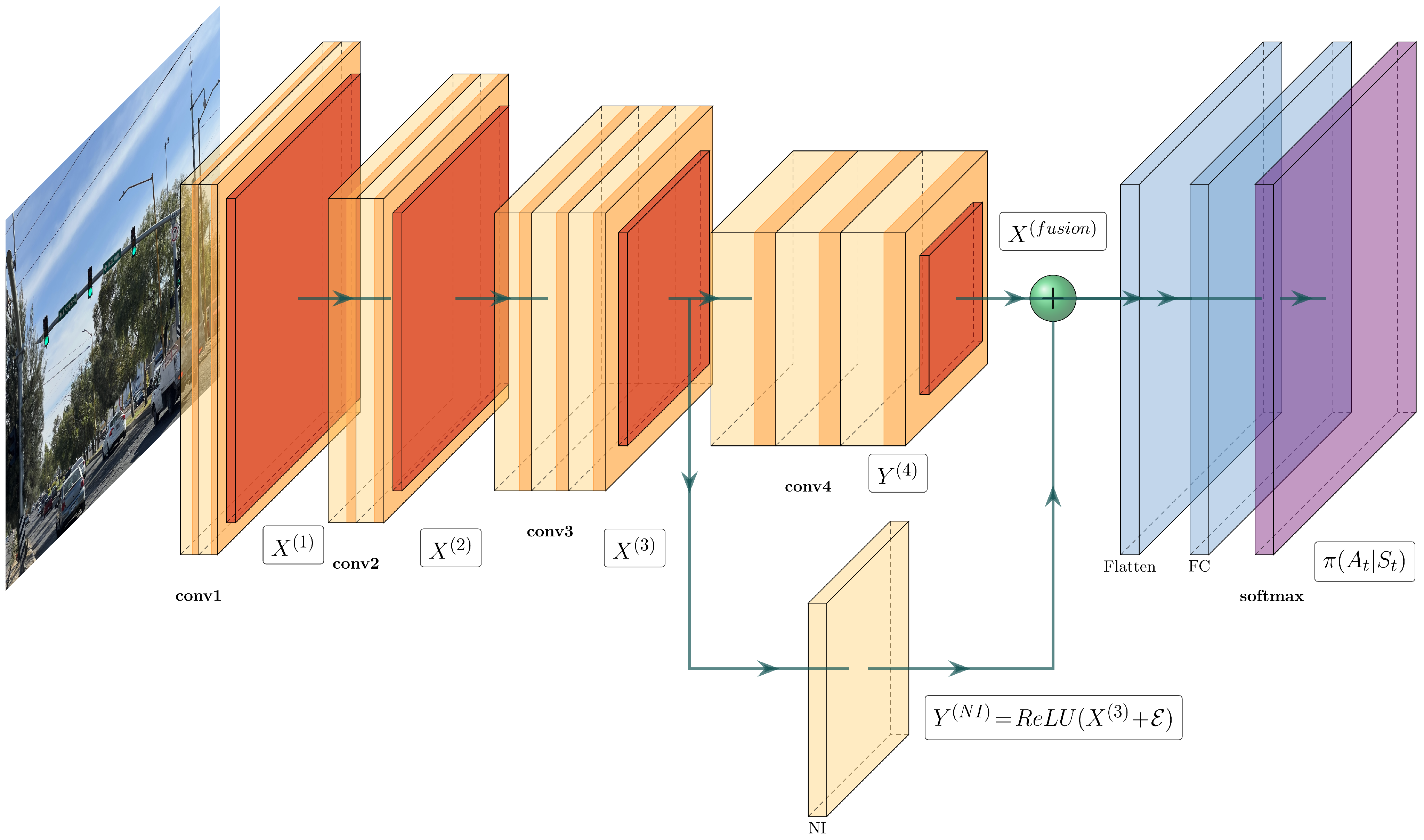
In this section, we formulate the ATSC problem as a DRL task, making a clear definition of all elements, such as scenario behavior, reward function, actions, and states. We present the functions used, such as experience replay (ER) and DQN, and explain the training with NI and DRL. The general architecture is illustrated in Figure 1, where the model is named ATSC-DRLNI, while

Table 1. Symbols used in the implementation of the decentralized DRL framework (ATSC-DRLNI) architecture.

Symbol	Meaning
s	State
a	Action
R	Reward
E	Environment
A	Agent
N	North
S	South
E	East
W	West
QL	Deep Q-Network (DQN)
T	Time frame
$G_l$	Green Light
$Y_l$	Yellow Light
$R_l$	Red Light
conv	Convolutional neural network

contains the notation used in this proposal.

3.1. System Description

The ATSC-DRLNI model is based on the joint implementation of techniques belonging to DRL and includes the CNN design, the data set (synthetic or real) processing, and the use of RL algorithms, in this case, ER and $\epsilon$-greedy policy. The general architecture is shown in Figure 1 and will be explained below and in the following sections.

The DL scheme is divided into two streams, one where the inputs are processed by four CNN layers connected in series and another where the output of the third CNN is passed through a NI-layer, where GN is incorporated, whose output is added to the output of the fourth CNN. The NI-layer will improve the behavior of the network, specifically with regularization, robustness, and performance. This NI-layer implements a rectified linear unit function (ReLU) that generates a flow with a discrete probability distribution. The final output vector is used in (i) the reward function, (ii) to update the CNN weights with back-propagation at each step using the DQN algorithm, and (iii) to create the batches and buffers to be used for ER learning. Finally, the $\epsilon$-greedy algorithm selects the actions.

In the selected DL architecture shown in Figure 1, there is a bifurcation in $X^{\left(3\right)}$, the output tensor map of spatial features recovered in the third CNN. The first branch of this bifurcation is sent directly to the fourth CNN to further extract high-level spatial features and produce a new output tensor map, $Y^{\left(4\right)}$. The other branch is directed to the NI layer, where, as explained before, random GN $\mathcal{E}\sim \mathcal{N}(0,{\sigma }^2)$ is added to tensor $X^{\left(3\right)}$ and then passed through a ReLU, which imposes a strict threshold ($max(0,x)$) to eliminate weak negative activation signals that may be produced by the injected GN $\mathcal{E}$. The output of the NI layer is the tensor $Y^{\left(NI\right)}=\mathrm{ReLU}(X^{\left(3\right)}+\mathcal{E})$. Finally, the output tensors of the $conv4$ and $NI$ layers in Figure 1 are fused by direct sum, $X^{\left(fusion\right)}=Y^{\left(4\right)}\oplus Y^{\left(NI\right)}$, and then passed through three layers: Flatten, FC, and softmax in Figure 1. The last layer, $softmax$, implements the policy $\pi \left(A_t\right|S_t)$ used in the A2C algorithm, and its output corresponds to the final result of the algorithm.

To stabilize the training process and ensure optimal convergence, the ATSC-DRLNI model includes an ER buffer and an $ϵ$-greedy action selection strategy with exponential decay. In the signal traffic control context, sequential traffic states are highly correlated, as the queue length at time t depends heavily on that at time $t-1$. Feeding these highly correlated successive sequential states directly to the CNN induces high variance in the CNN output and instability in its behavior. To address this issue, the ER mechanism uses a finite-capacity buffer $\mathcal{B}$ that stores agent experiences as transition tuples $e_t=(S_t,A_t,R_t,S_{t+1})$. At each learning step, mini-batches of tuples of uniform size are randomly sampled from buffer $\mathcal{B}$. This random sampling breaks the time correlation and allows the DQN algorithm to update network weights more stably.

As mentioned, action selection is based on an $ϵ$-greedy strategy that allows us to obtain a trade-off between exploration and exploitation of the search space. This allows the agent to freely explore various phase synchronization combinations in the early stages of the learning and to exploit the learned Q values when convergence is near. The rate of exploration $ϵ$ decays exponentially with training episodes according to

$${ϵ}_e={ϵ}_{ending}+({ϵ}_{starting}-{ϵ}_{ending})·exp(-e/\tau ),$$

where e represents the current episode, and $\tau$ is a constant that determines the speed of decay. The initial value of the exploration rate is ${ϵ}_{starting}=1.0$, which is aggressively reduced to reach a final value of ${ϵ}_{ending}=0.05$, which guarantees that the end agent depends largely on the optimized policy of the final episodes.

3.2. Actions

The set of feasible actions include all possible signals that a traffic light can adopt and, therefore, that an agent is free to choose from. For example, suppose that a traffic light change may occur within a given time frame T, and the agent starts a cycle with the green phase of the traffic light ($G_l$), then, depending on the state of traffic, the agent will move to the yellow phase ($Y_l$) and, finally, to the red phase of the traffic light ($R_l$). To maintain a stable vehicular flow, after a time for $R_l$, the agent should switch back to the $G_l$ to repeat the cycle, noting that only one phase can be active at any time. Action ($G_l$, $Y_l$, $R_l$) of agent A at time t is denoted by $A_t$.

3.3. States

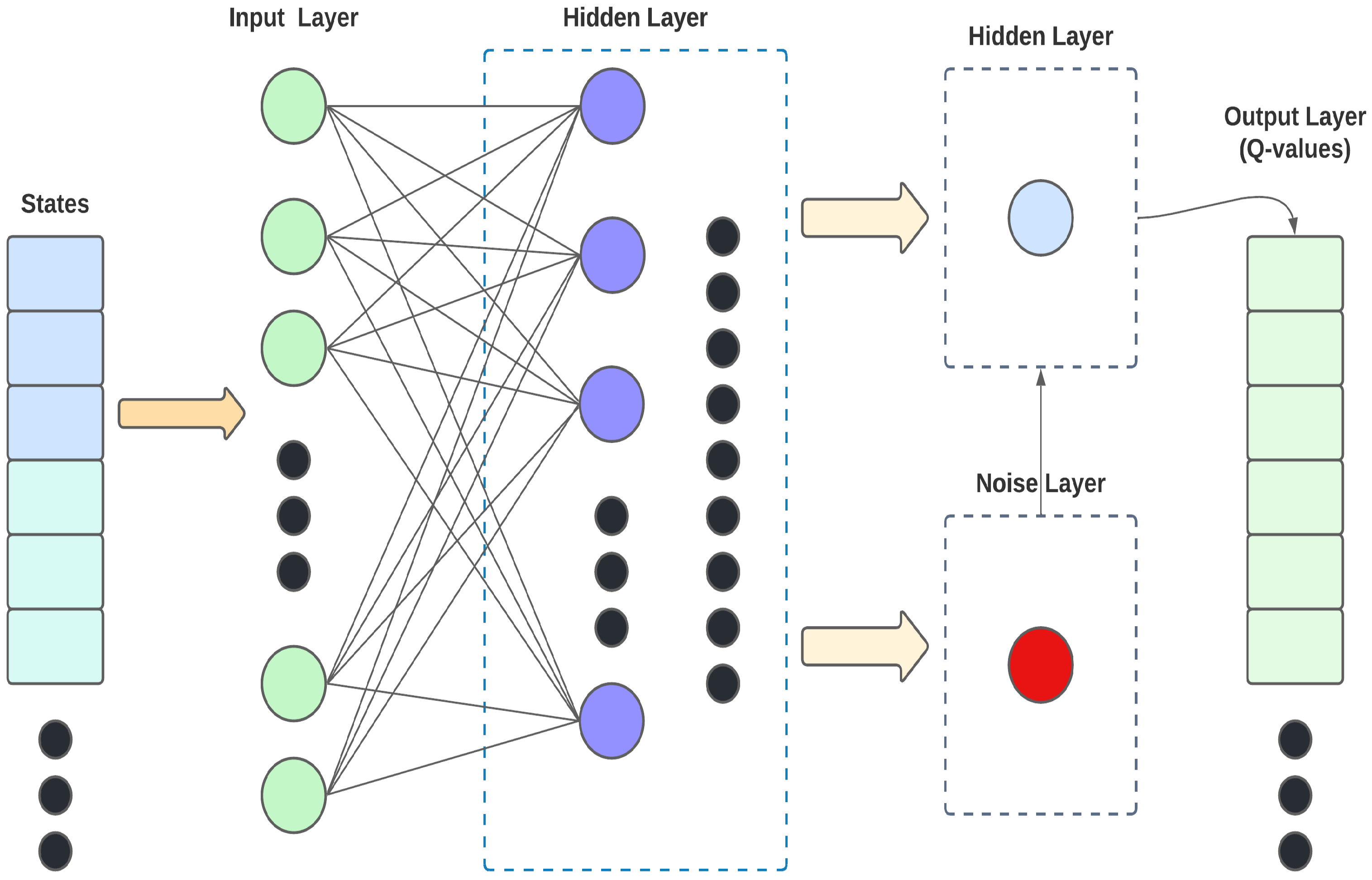
The state at time t, where an action is taken, is formed as a vector whose elements contain information from the environment, which is given by the specific features obtained from the traffic light sensors in use (length of vehicles, vehicle density, the distance between stopped and moving vehicles, etc). In our case, we use as information the total number of vehicles at a distance D from the intersection under analysis and associate this number also with the actions of the traffic light signals, e.g., $G_l$, $Y_l$, and $R_l$ and their respective time frames. Figure 2 illustrates the data flow from states to Q-values.

3.4. Reward

The reward function is an essential component of the RL algorithm design, since it is the feedback index that evaluates the quality of the agent’s performance.

We implement a reward function at time t, $R_t$, based on the combination of the vehicle queue, flickers, and the agent action $A_t$ as follows:

$$R_t=-{\displaystyle \frac{1}{p\left(A_t\right)}}·{\displaystyle \frac{Q_t}{Q_{norm}}}-{\displaystyle \frac{F_t}{F_{norm}}},$$

(6)

where $p\left(A_t\right)$ is the probability of action $A_t$, decided in the A2C policy described below, $Q_t$ the size of the vehicle’s queue in the scenario considered, and $F_t$ the number of flickers at time t. $Q_{norm}$ and $F_{norm}$ are appropriate factors to scale the variables involved.

This reward function has an additional penalty included when there are no vehicles and a flicker is produced, in that case,

$$R_t\leftarrow R_t-F_p$$

(7)

with $F_p$ the chosen penalty. The proposed reward then weighs the length of the queue and the number of flickers. A positive change in the reward indicates an improvement in the intersection condition, and conversely, a negative change in the reward shows deterioration. The reward function is used by the agents, in this case, the traffic lights involved in the scenario that will be introduced later on, and the interaction with the environment determines the policy of each agent. This reward function uses the DQN function presented before. To detect changes in the reward, the following time difference is introduced:

$$S_t=R_t-R_{t-1}$$

(8)

3.5. The Neural Network Structure

The structure of the proposed NN model is illustrated in Figure 2. This NN is designed in such a way that it can process any state and produce a proper action. The input received comes from video cameras installed at several points before the intersection that, once processed, provide information about the number of vehicles at a certain distance D of the intersection for the considered scenario, to be detailed further on. There are four CNN hidden layers aiming to maintain an adequate performance both in the NN and in the pre-processing. These layers include a NI-layer with a ReLU activation function. The number of output nodes for obtaining the Q-values functions is equivalent to the number of actions, which, in turn, are the triggers for obtaining the best reward. The NI-layer provides a statistical probability distribution by means of GN, which is added to the result of the last CNN. The output layer vector is the set of Q-values used to minimize the updating function $Q_t$ in Equation (4). Algorithm 1 describes the A2C policy optimization in the ATSC-DRLNI model.    

Algorithm 1: ATSC-DRLNI policy optimization

The policy ${\Pi }_0$ is initialized with a random stochastic value to calculate the function $S_0$. Then, given a state $S_t$ and an action $A_t$ carried out, the policy at time t, ${\Pi }_t$ is determined. The reward time difference is computed in step 3 of the algorithm, where the goal is to adjust $S_t$ using $R_t$, the current value of the reward, and the previous value $S_{t-1}$. The term ${\delta }_t$ = $R_t+\gamma S_{t-1}-S_t$ in step 4 of the A2C algorithm represents the time difference error function, which serves as an estimator in the critic component of the algorithm. The function ${\delta }_t$ is essential for learning, as it evaluates the outcome based on the reward of the chosen action. When ${\delta }_t>0$, it indicates that the probability of taking action At should be increased; conversely, if it is negative, the probability of taking action At should be decreased, because choosing it leads to poorer performance in the objective function.

Updating the critic will adjust the estimated value of $S_t$ using $S_{t-1}$ and $\alpha$, the learning ratio of the critic, not the actor. Finally, the new state must be set, and the algorithm is repeated from step 2.

4. Experimental Results and Analysis

In this section, the scenarios and dataset for the simulation are established. To verify the performance of our proposal, simulation results comparing them with other well-established methods available in the open literature are presented. A summary of the statistics of the general behavior obtained is also included.

4.1. Experimental Setup

To validate the functionality of the methodology, several simulations were carried out for different scenarios and behaviors of vehicular traffic. The simulations were coded with the Simulation of Urban MObility (SUMO) sumo-gui version 1.10.0 platform, Python 3.8.8, and OpenAI Gym version 0.7.4 and executed in a cluster with the following technical data: MSI Intel(R) Core(TM) i7- 10870H CPU @ 2.20GHz, 16GB DDR5 RAM, VRAM 8GB DDR6 NVIDIA RTX3600, and 3060 NVIDIA CUDA Core. Relevant intersection data used for the simulations are shown in

Table 2. Intersection parameters.

Parameter	Value
Number of lanes	10
Traffic Flow	Random trips
Simulation platform	SUMO
Yellow phase duration	5 s
Initial Green phase duration	30 s
Distance D to intersection to detect vehicles	800 m
Value of $Q_{norm}$	5000 vehicles
Value of $F_{norm}$	100 flicker
Value of $F_p$	0.2 flicker

.

4.1.1. Simulation Environment and Dataset

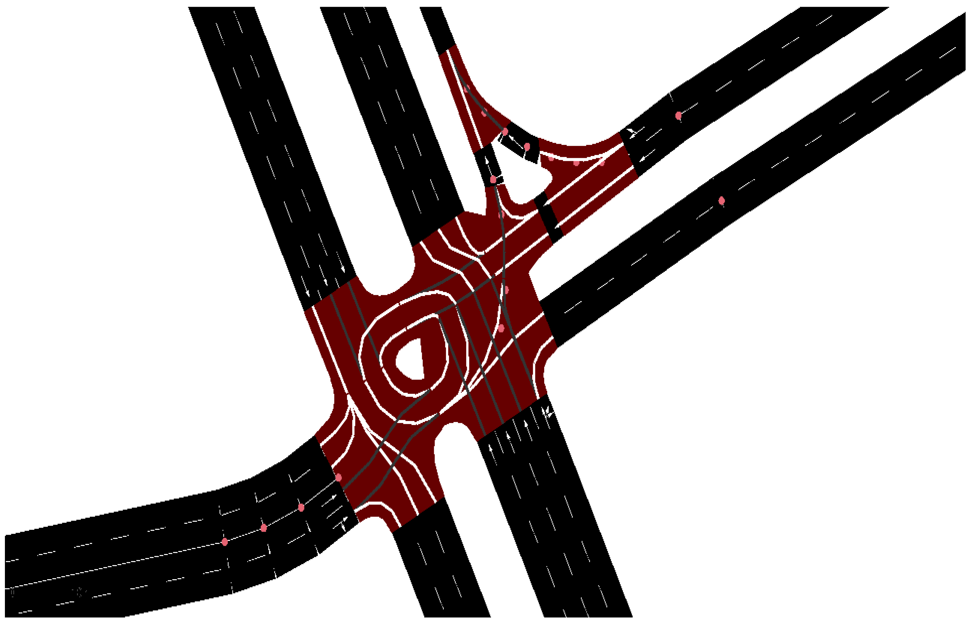
The traffic intersection depicted in Figure 3 is the environment used to train the RL algorithm. It represents an intersection in Aguascalientes, a city in Mexico, where the empirical data set was provided by the local Dirección de Tránsito y Vialidad and was obtained by an intelligent traffic system provided with cameras and sensors. Vehicle directions in the intersection are $N,S,E,W$, indicated as $N\leftrightarrow S$ and $E\leftrightarrow W$, implying that both directions are valid at the same time. Vehicle directions also include turns, as vehicles can go from S to W ($S\to W$) and from N to E ($N\to E$).

The intersection has four traffic light phases with the following directions: Phase 1 (north–south) and (south–north); Phase 2 (east–west) and (west–east); Phase 3 (east–south) and (north–east); Phase 4 (east–north) and (west–north). To ensure that the model learns from a robust variety of traffic patterns, the dataset corresponds to a complete week (Monday to Sunday), allowing the capture of both weekday and weekend dynamics. Data samples, providing high-resolution information on traffic conditions at the intersection, were collected at 30-s intervals. For training purposes, three 4-h subsets were extracted from the dataset of each day, with each subset representing distinct and realistic traffic conditions.

• Off-peak conditions (normal traffic): representing free-flow traffic, characterized by lower average vehicular density and a lower stochastic vehicle arrival rate.
• Peak conditions (congested traffic): representing high-demand traffic characterized by the presence of congestion. Empirical data indicate that traffic volume reaches approximately 400 vehicles per complete traffic light cycle (green–yellow–red).

To reduce the gap between empirical and simulation data, vehicle generation in SUMO was probabilistically defined to match real sensor measurements collected at 30-s intervals, accounting for vehicles traveling straight as well as those making left and right turns. In this way, the DRL algorithm was trained using realistic traffic data representing both free-flow and congested conditions.

Two scenarios were simulated: in the first one, phases 1 and 2 are optimized to give preference to straight traffic, while the second optimization is based on phases 3 and 4, which favor more complex maneuvers (turns to right and left) that are, in general, more prone to cause congestion. Special configurations for the right and left lanes, where vehicles execute turns, were also defined with the intention of representing real situations at urban intersections, where turns are a critical issue in traffic handling.

The training process inherently captured the temporal variability of urban traffic by using blocks of four-hour sensor data, collected at 30-s resolution, over a full week, enabling the ATSC-DRLNI model to learn transitions between free-flow and congested traffic. Since the empirical dataset did not include information on pedestrian presence or emergency vehicles, these factors were not considered in the current study. Nevertheless, the proposed decentralized architecture provides a foundation for extending the state representation. Future work will incorporate vulnerable road users and emergency vehicle prioritization by expanding the observation vector within a multi-agent framework.

The distance $D=800$ m, selected to detect incoming vehicles to the intersection, represents a typical urban environment with relatively short distances between intersections and poses an additional challenge for the synchronization of traffic lights.

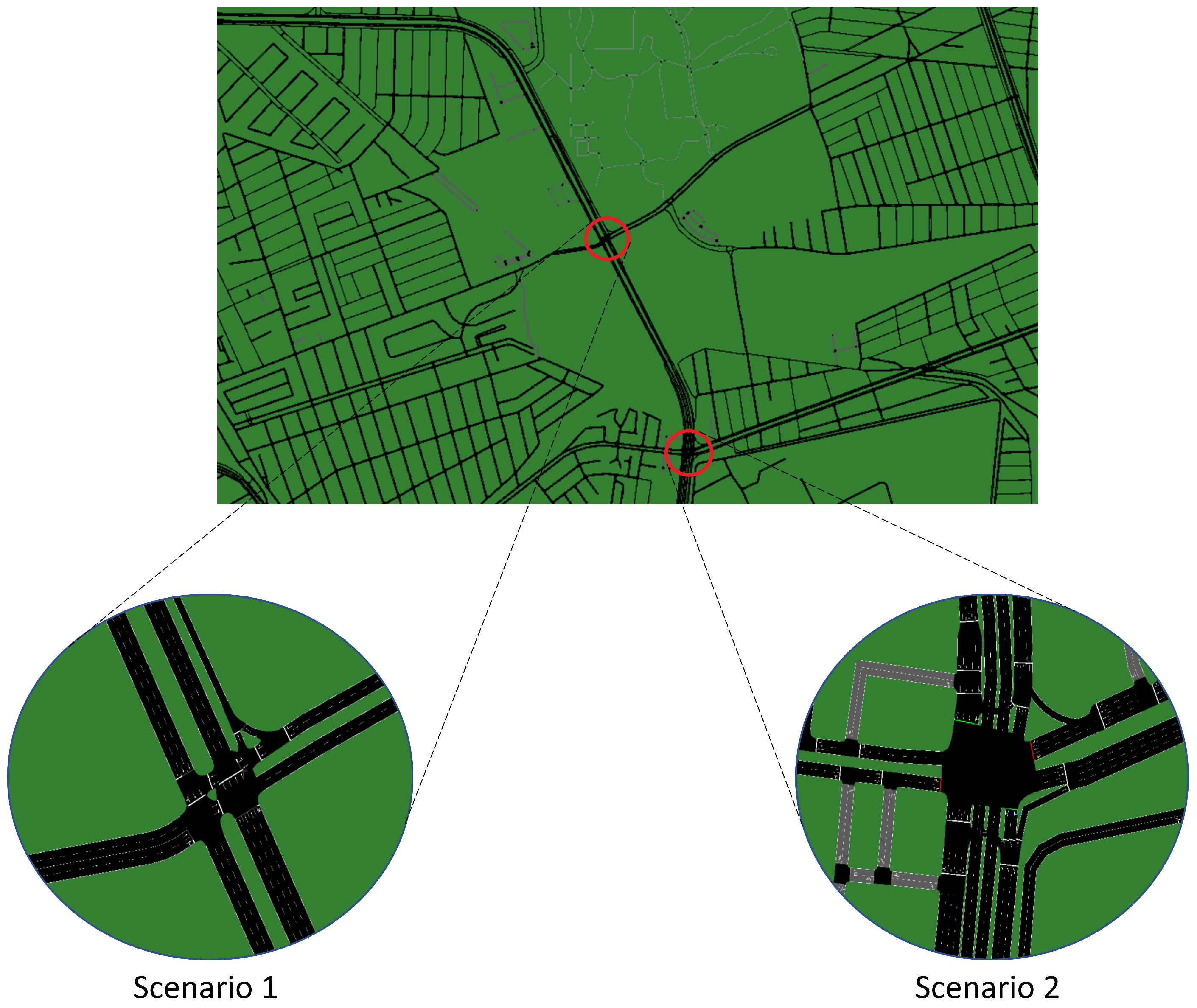
Once trained, the ATSC-DRLNI model was applied to the two environments shown in Figure 4, with

Table 3. Intersection scenario 1 parameters.

Parameter	Value
Number of lanes	10
Traffic Flow	Random trips
Simulation platform	SUMO
Yellow phase duration	5 s
Initial Green phase duration	30 s
Distance D to intersection to detect vehicles	800 m
Value of $Q_{norm}$	5000 vehicles
Value of $F_{norm}$	100 flicker
Value of $F_p$	0.2 flicker

and

Table 4. Intersection scenario 2 parameters.

Parameter	Value
Number of lanes	14
Traffic Flow	Random trips
Simulation platform	SUMO
Yellow phase duration	5 s
Initial Green phase duration	30 s
Distance D to intersection to detect vehicles	800 m
Value of $Q_{norm}$	6500 vehicles
Value of $F_{norm}$	100 flicker
Value of $F_p$	0.2 flicker

showing the corresponding parameters. The same 4 phases and scenarios used for training still apply. However, we used the data for a complete week, obtained from the same source. The results shown below correspond to scenario 1, where phases 1 and 2 are optimized to give preference to straight traffic, as better results were obtained with this scenario.

4.1.2. Selected Methods for Comparison

Seven other traffic control methods were selected from the open literature to use for comparison purposes with the proposal of this work, which are listed below. In all of them, the same scenarios and reward function, where applicable, were used.

• Fixed-Time (FT): This is a classical non-adaptive method used for traffic light control that serves as a baseline for comparisons.
• Multi-Agent Deep Reinforcement Learning (MADRL): Multi-agent algorithm based on DRL. It uses gradient policies and trains agents in a centralized manner, where collective decision-making is based on real-time information feedback to agents. There are also decentralized versions, where agents are autonomous with decision-making not depending on other agents.
• Multi-Agent Recurrent Deep Deterministic Policy Gradient (MARDDPG): decentralized algorithm for agent training where each agent shares policies and information with other agents. Individual agents are capable of executing decision independently.
• Single-Agent-Based Algorithm (SABA): DQN-based decentralized algorithm where agents do not relate between them, although they try to predict what other agents may decide.
• Longest Queue First (LQF): This method favors lane selection where the green light is already active and gives priority to vehicles close to the intersection, a situation that may produce inconsistent phase cycles.
• Q-Learning (DQN): RL-based method for action learning that uses a predefined number of Q-values that are related to the number of actions. Actions are stored in a table that contains elements, such as vehicle queue, waiting time of vehicles in lanes close to the intersection, and the current phase.
• Self-Organizing Traffic Lights (SOTL): This method uses a self organizing algorithm to determine the phases of the traffic lights.

4.2. Comparative Simulation Results

Simulations use the parameters shown in

Table 5. Description of model parameter used in simulations.

Parameter	Description
Batch size	Number of samples used at each iteration to determine the NN error.
Neural network layers	Number of NN layers to identify patterns or characteristics of the input data.
Hidden layers	Number of intermediate layers to process the information between input and output.
Noise injection (NI) layer	Layer to introduce Gaussian noise (GN) to improve model generalization.
Activation function	Non linear function that determines the output of each neuron. ReLU is the most used because of its high computational efficiency and capacity to mitigate the gradient vanishing problem.
Learning rate	Rate controlling the size of weight adjustment during NN training, based on previous reward values.
Discount factor	Factor that determines the importance of future rewards in comparison with past rewards.
Optimizer	Algorithm to adjust NN parameters and to control convergence speed during training.
Episode	Total number of simulation episodes to be executed during training.
Epsilon starting	Initial value of exploration parameter $ϵ$ for the $ϵ$-greedy strategy.
Epsilon ending	Final value of exploration parameter $ϵ$ for the $ϵ$-greedy strategy, after exponential decay.

. The values that yielded the best results in terms of the final value of the metrics, convergence, and stability are included in

Table 6. Simulation parameters for traffic light control training simulations.

DQN Model Simulation Parameters
Parameter	Value
Batch size	32
Neural network layers	4
Number of Hidden Layers	3
Noise injection layers (GN)	1
Activation function	ReLU
Learning rate	$1\times {10}^{-4}$
Discount factor	0.99
Optimizer	Adam
Episodes	5000
Epsilon starting	1.0
Epsilon ending	0.05

.

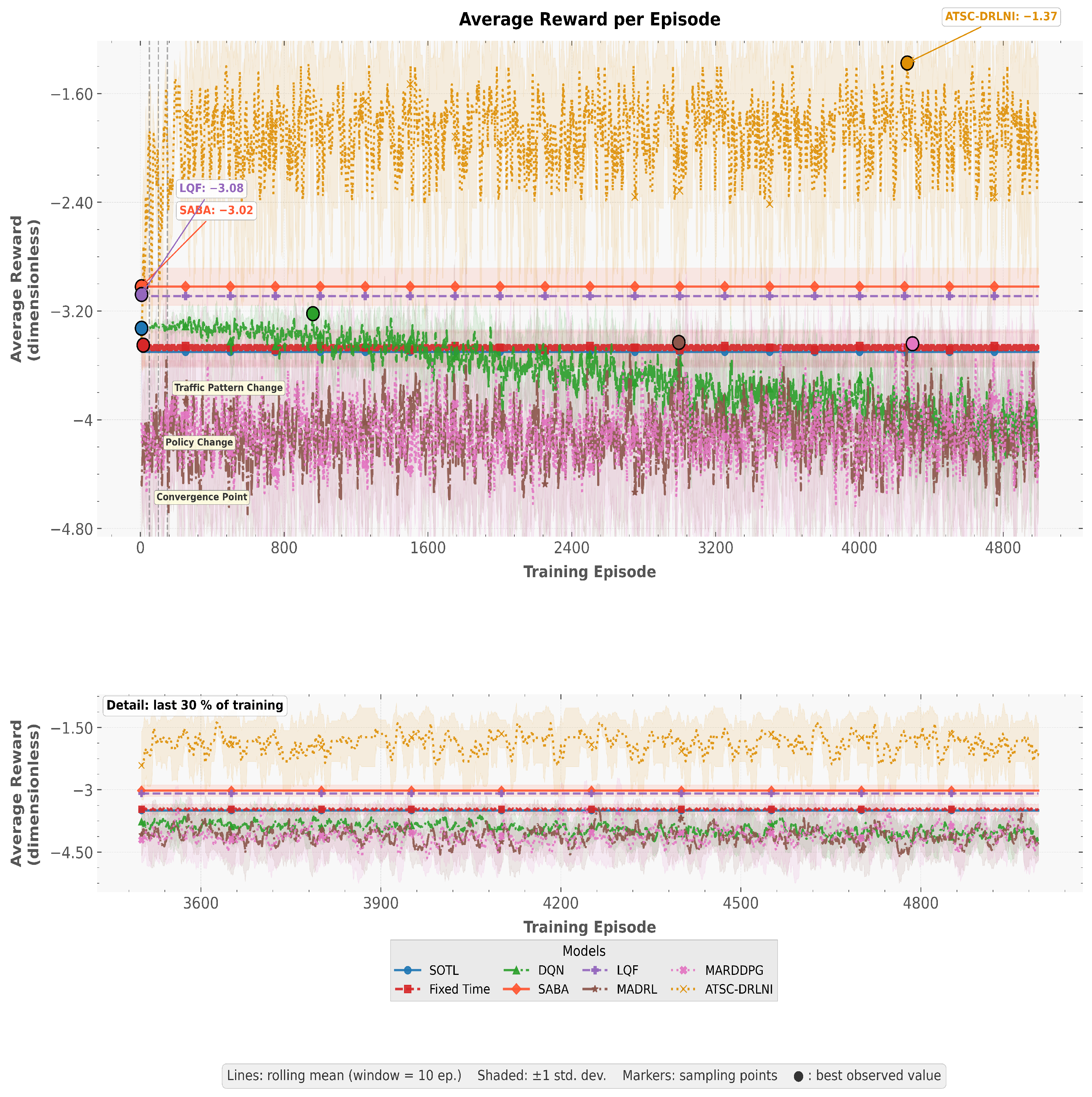
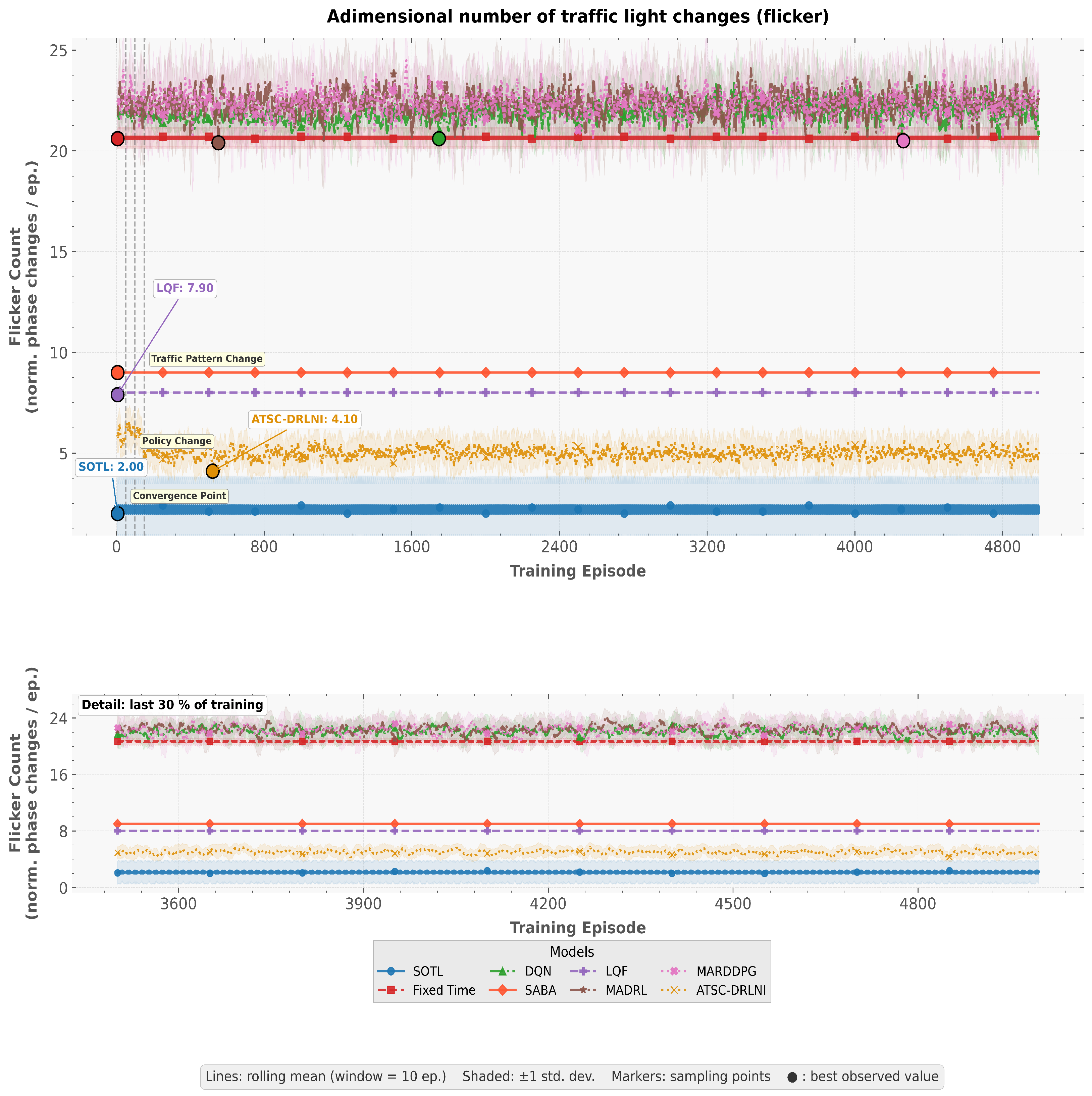
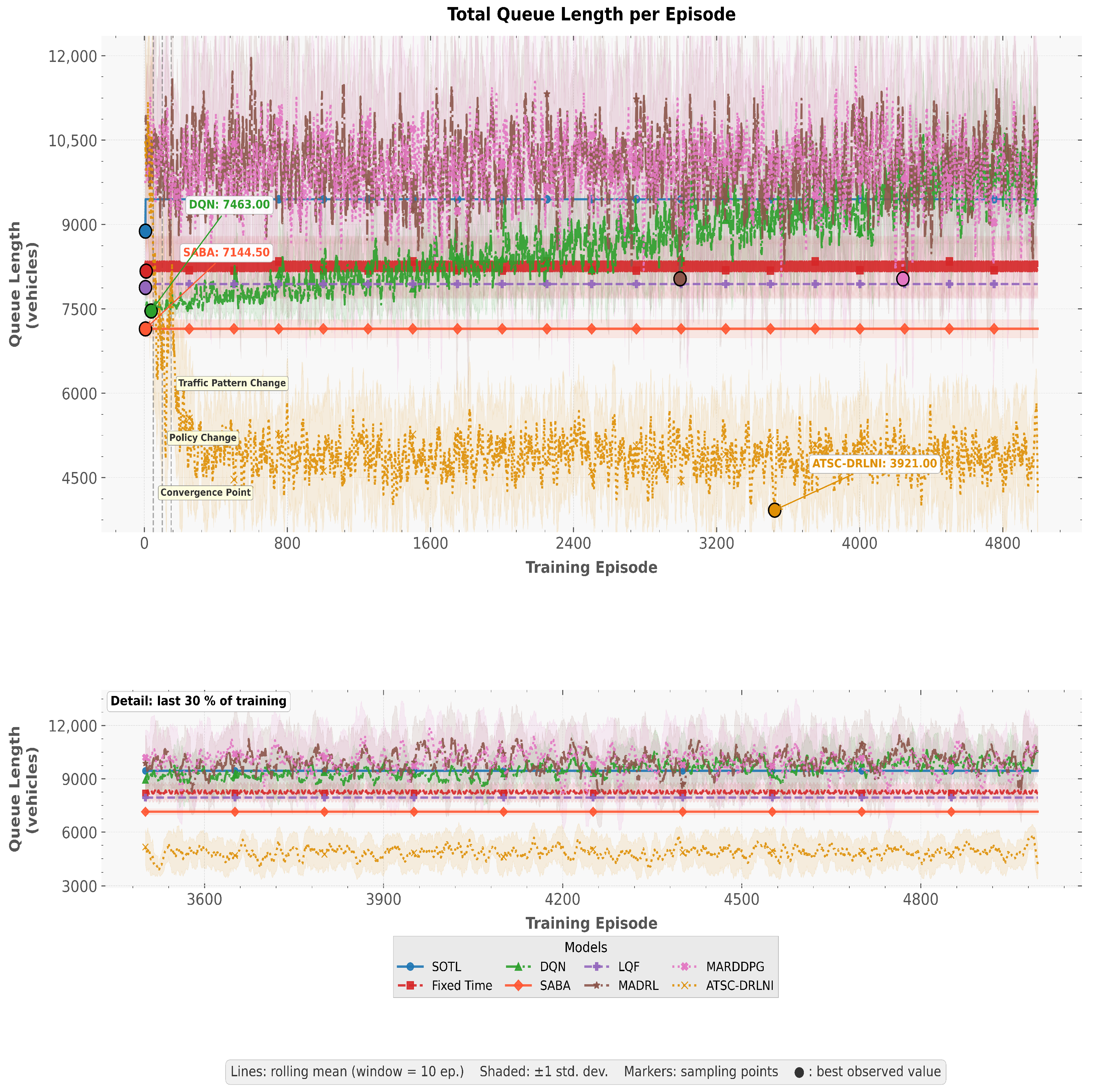
The results of applying the model are represented using different metrics: average waiting time (AWT), average queue length (AQL), average reward (AR), and traffic light changes (flickers), this one divided by $F_{norm}$. Figure 5, Figure 6 and Figure 7 show an example of one simulation of 5000 episodes, where the AR, AQL, and flickers are plotted against the number of episodes for all the eight models considered. In all cases, they are plotted using a moving average with a window of 10 episodes and a shadow area representing the standard deviation and correspond to a complete week of traffic data at the two intersections under consideration.

In Figure 5, the final value of the AR obtained with ATSC-DRLNI is higher than that of any other model; it is 38% better than the closest model, SABA. The AR value begins at −3.18 and ends at −1.80, showing a large variation in the first 300 episodes. SABA and LQF, non RL models, achieve a much faster convergence; however, their final AR values are −3.02 and −3.08, respectively. In the case of DQN, it has acceptable initial AR values; however, it shows a poor learning capacity, finishing with a value of −4.3, similar to those obtained with MARDDPG and MADRL.

The queue length for the eight models is presented in Figure 6, expressed in total vehicles. For ATSC-DRLNI, the value converges to 2426 vehicles. This value is significantly smaller (40%) than those achieved by SABA, SOTL, LQF, and FT, which attain intermediate queue length results. The other models, MARDDPG, MADRL, and DQN, have the worst queue length results.

With respect to the adimensional number of flickers in Figure 7, the best results were obtained by SOTL, followed by ATSC-DRLNI, which compares favorably with the other six models, where LQF and SABA perform only slightly worse than ATSC-DRLNI.

A summary of the results for the metrics considered is included in

Table 7. Complete training results for the 8 tested models.

Metrics	Methods
	DQN	SABA	MARDDPG	MADRL	LQF	FT	SOTL	ATSC-DRLNI
AQL_mean	4341.726	3572.250	4994.691	5004.292	3970.439	4117.582	4723.433	2497.479
AQL_std	596.119	164.266	983.944	993.988	6.435	242.440	55.359	675.804
AQL_final	4708.643	3572.250	4992.671	4986.901	3970.500	4117.548	4724.000	2426.285
AWT_mean	2170.863	1786.125	2497.345	2502.146	1985.220	2058.791	2361.716	1248.739
AWT_std	298.059	82.133	491.972	496.994	3.217	121.220	27.680	337.902
Reward_mean	−3.661	−3.020	−4.103	−4.112	−3.090	−3.472	−3.500	−1.902
Reward_std	0.368	0.130	0.577	0.583	0.002	0.118	0.025	0.648
Reward_final	−3.912	−3.020	−4.100	−4.101	−3.090	−3.472	−3.500	−1.874
Flicker_mean	21.885	9.000	22.328	22.340	8.000	20.666	0.001	5.024
Flicker_std	1.199	0.000	1.738	1.757	0.014	0.472	0.042	0.832

, which includes mean values, final values, and standard deviation during the last episode.

Three different metrics to show learning stability, traffic balance, and system stability were also obtained based on the following definitions:

$$\begin{array}{cc}\hfill Learning\_stability& =1-min\left(1,{\displaystyle \frac{{\sigma }_{R_{late}}}{|{\mu }_{R_{late}}|+ϵ}}\right)\hfill \end{array}$$

(9)

with

$$\begin{array}{cc}\hfill R_{late}& \{r_i:i\ge 3000\}\mathrm{reward}\mathrm{in}\mathrm{final}\mathrm{episodes}\hfill \end{array}$$

(10)

$$\begin{array}{cc}\hfill {\mu }_{R_{late}}& ={\displaystyle \frac{1}{|R_{late}|}}\sum _{r\in R_{late}}r\hfill \end{array}$$

(11)

$$\begin{array}{cc}\hfill {\sigma }_{R_{late}}& =\sqrt{{\displaystyle \frac{1}{|R_{late}|-1}}\sum _{r\in R_{late}}{(r-{\mu }_{R_{late}})}^2}\hfill \end{array}$$

(12)

where $ϵ=0.1$ is a regularization factor that prevents large values in the division in cases where the mean is close to zero and helps to obtain computational stability. The chosen value, 0.1, was adjusted according to the agent’s reward, yielding regularization without inducing bias in the stability metrics for all the considered models.

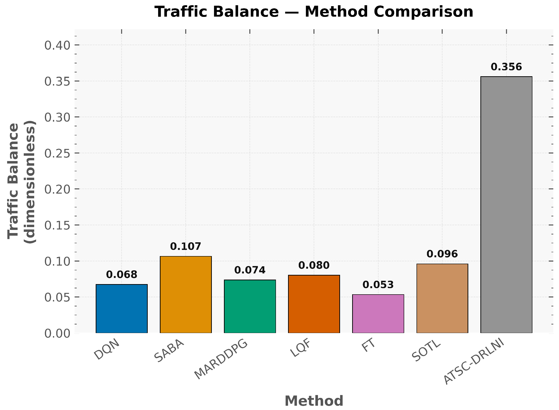
$$\begin{array}{cc}\hfill Traffic\_balance& =1-{\displaystyle \frac{|{\mu }_{Q_{NS}}-{\mu }_{Q_{EW}}|}{max(0.1,{\mu }_{Q_{NS}}+{\mu }_{Q_{EW}})}}\hfill \end{array}$$

(13)

with ${\mu }_{Q_{NS}}$ mean vehicle queue size in the north–south direction and ${\mu }_{Q_{EW}}$ mean vehicle queue size in the east–west direction.

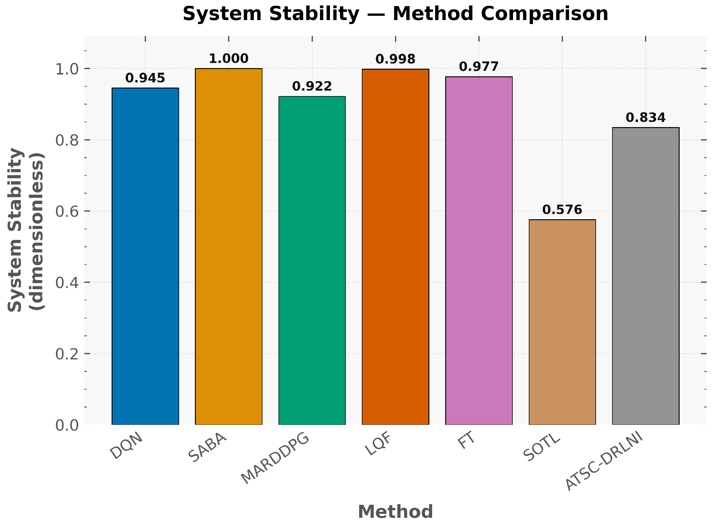
$$\begin{array}{cc}\hfill System\_stability& =1-{\displaystyle \frac{{\sigma }_{flicker}}{max(0.1,{\mu }_{flicker})}}\hfill \end{array}$$

(14)

where ${\mu }_{flicker}$ is the mean value of the flickers, and ${\sigma }_{flicker}$ is its standard deviation.

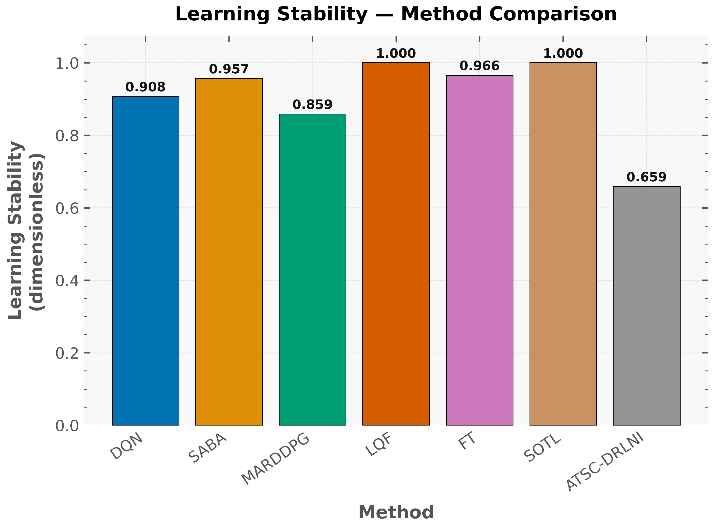
The values of these three metrics are shown in Figure 8, Figure 9 and Figure 10 where, in all cases, the closer the value to 1, the better the metric. It can be noted that the ATSC-DRLNI performs best in terms of traffic balance and worse in terms of learning stability, an issue that will be commented on below. Its performance in terms of system stability is similar to the other methods.

4.3. Sensitivity Analysis for ${\sigma }^2$ Selection

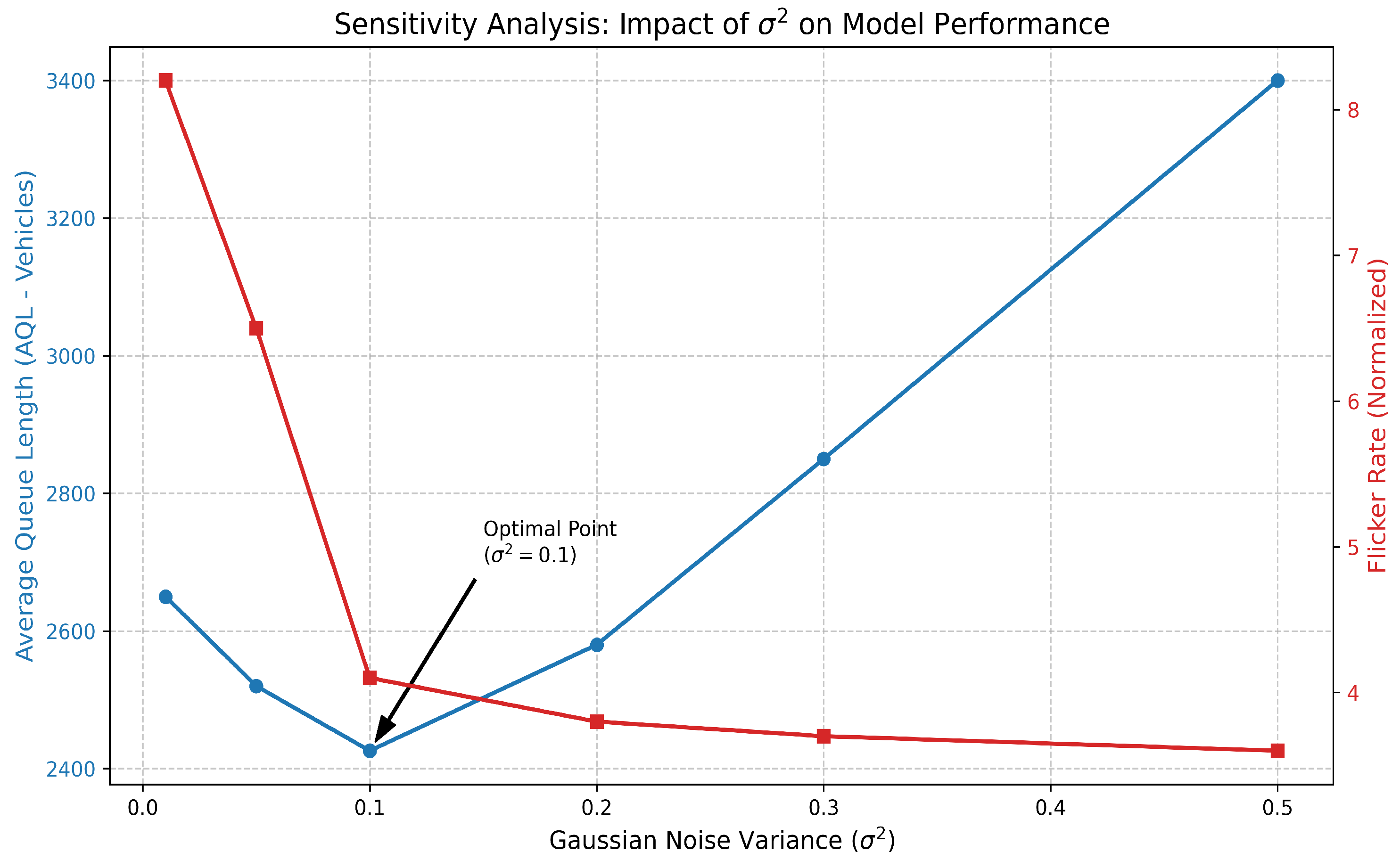
To further support the design choices introduced in the previous subsections, a sensitivity analysis was conducted to validate the selection of the variance parameter ${\sigma }^2$ in the NI layer, which was used in all simulations. The performance of the ATSC-DRLNI model was evaluated for values of ${\sigma }^2\in [0.01,0.5]$. Results indicate that lower values (${\sigma }^2<0.05$) do not provide sufficient regularization and lead to a $5\%$ increase in flicker events, as agents overreact to small stochastic fluctuations. Conversely, excessively high values (${\sigma }^2>0.3$) deteriorate the reward signal, making convergence more difficult and increasing the AQL. Figure 11 presents the results of this ${\sigma }^2$ sensitivity analysis for both AQL and flicker rate, showing that the global minimum of the AQL is achieved at ${\sigma }^2=0.1$, corresponding to a queue length of 2426 vehicles.

4.4. Reward Function Component Interaction Analysis

4.4.1. Overall Pearson Correlation Analysis

Additionally, a correlation analysis was conducted to explore the interactions among the components of the reward function and to assess potential trade-offs between stability and efficiency. The Pearson correlation coefficient r was used to measure the strength and direction of the linear relationship between pairs of performance metrics. The magnitude of r was classified according to the scale proposed by Evans [76], which is widely accepted in the context of complex systems:

• $r\in$ [0.00–0.19]: Very weak.
• $r\in$ [0.20–0.39]: Weak.
• $r\in$ [0.40–0.59]: Moderate.
• $r\in$ [0.60–0.79]: Strong.
• $r\in$ [0.80–1.00]: Very strong.

To evaluate the relationship between traffic lights stability and the operational efficiency of the ATSC-DRLNI model, four metrics were computed over 5000 simulation episodes with the ATSC-DRLNI model already trained for environments 2 and 3, shown in Figure 4, where the key metrics obtained after the episodes are shown in

Table 8. Comparison of obtained key metrics in simulations of 5000 episodes for environments 2 and 3 of all evaluated models.

Model	Flickers Mean	AQL Mean	Mean Reward
ATSC-DRLNI	5.02	4995	−1.90
SABA	9.00	7145	−3.02
LQF	8.00	7941	−3.09
Fixed Time	20.67	8235	−3.47
DQN	21.89	8683	−3.66
MARDDPG	22.33	9989	−4.10
MADRL	22.34	10,009	−4.11
SOTL	2.18	11,094	−4.12

. Pearson correlation coefficients were calculated for relevant metric pairs. The four metrics considered were (i) flickers; (ii) AQL; (iii) AWT; and (iv) average traveling time (ATT).

Table 9. Pearson correlation between ATSC-DRLNI performance metrics for 5000 episodes.

Metric Pair	Pearson r	Force	Interpretation
Flickers–AQL	$+0.10$	Very weak (+)	Flickers do not linearly determine congestion levels.
Flickers–AWT	$+0.07$	Very weak (+)	Flickers do not significantly affect waiting time.
Flickers–ATT	$+0.14$	Very weak (+)	Traveling time is independent of flickers.
AQL–AWT	$+0.92$	Strong (+)	Queue length is strongly correlated with waiting time.
AQL–ATT	$+0.78$	Strong (+)	Queue length associates positively with traveling time.

presents the results for five representative metric pairs.

The weak correlations observed between flickers and the three congestion-related metrics ($r\le +0.14$) indicate a practical decoupling between traffic light stability and operational efficiency. This contrasts with reactive traffic control policies such as SOTL (where aggressive stabilization strategies lead to substantially larger queues). In contrast, ATSC-DRLNI achieves a low number of flickers (mean = 5.0 2.18, AQL = 11,094), 2) while maintaining the smallest AQL among all comparison models (mean = 4995). These results suggest that the learned policy optimizes flicker quality rather than merely reducing its frequency and that incorporating flicker penalization into the reward function does not compromise overall traffic performance. Conversely, the strong correlations observed between AQL and AWT ($r=+0.92$) and between AQL and ATT ($r=+0.78$) confirm the internal consistency of the model and indicate that AQL is strongly associated with both waiting and traveling times.

Table 10. Pearson correlations between ATSC-DRLNI performance metrics by traffic regimen: Off-Peak and Peak.

Metric Pair	r Off-Peak $(\mathbf{n}=\mathbf{3252})$	r Peak $(\mathbf{n}=\mathbf{1748})$	r Global $(\mathbf{n}=\mathbf{5000})$	$\mathbf{\Delta }\mathit{r}$
Flickers–AQL	$+0.0196$	$+0.1629$	$+0.0959$	$+0.1433$
Flickers–AWT	$-0.0046$	$+0.1209$	$+0.0717$	$+0.1255$
Flickers–ATT	$+0.0889$	$+0.1979$	$+0.1377$	$+0.1090$
AQL–AWT	$+0.7631$	$+0.8945$	$+0.9153$	$+0.1314$
AQL–ATT	$+0.5463$	$+0.7414$	$+0.7839$	$+0.1952$

further confirms the robust performance of ATSC-DRLNI, demonstrating its ability to simultaneously maintain competitive AR, low AQL, and reduced flicker rates.

4.4.2. Pearson Correlation Under Off-Peak and Peak Traffic Conditions

As previously described, the ATSC-DRLNI model was trained using both off-peak and peak traffic data. To assess whether this combination influenced the observed relationships among performance metrics, the learning episodes were segmented using an AQL threshold of 5405 to distinguish off-peak from peak conditions. This threshold was selected to approximate typical traffic distributions, where peak periods represent approximately $35\%$ of a standard traffic day [17].

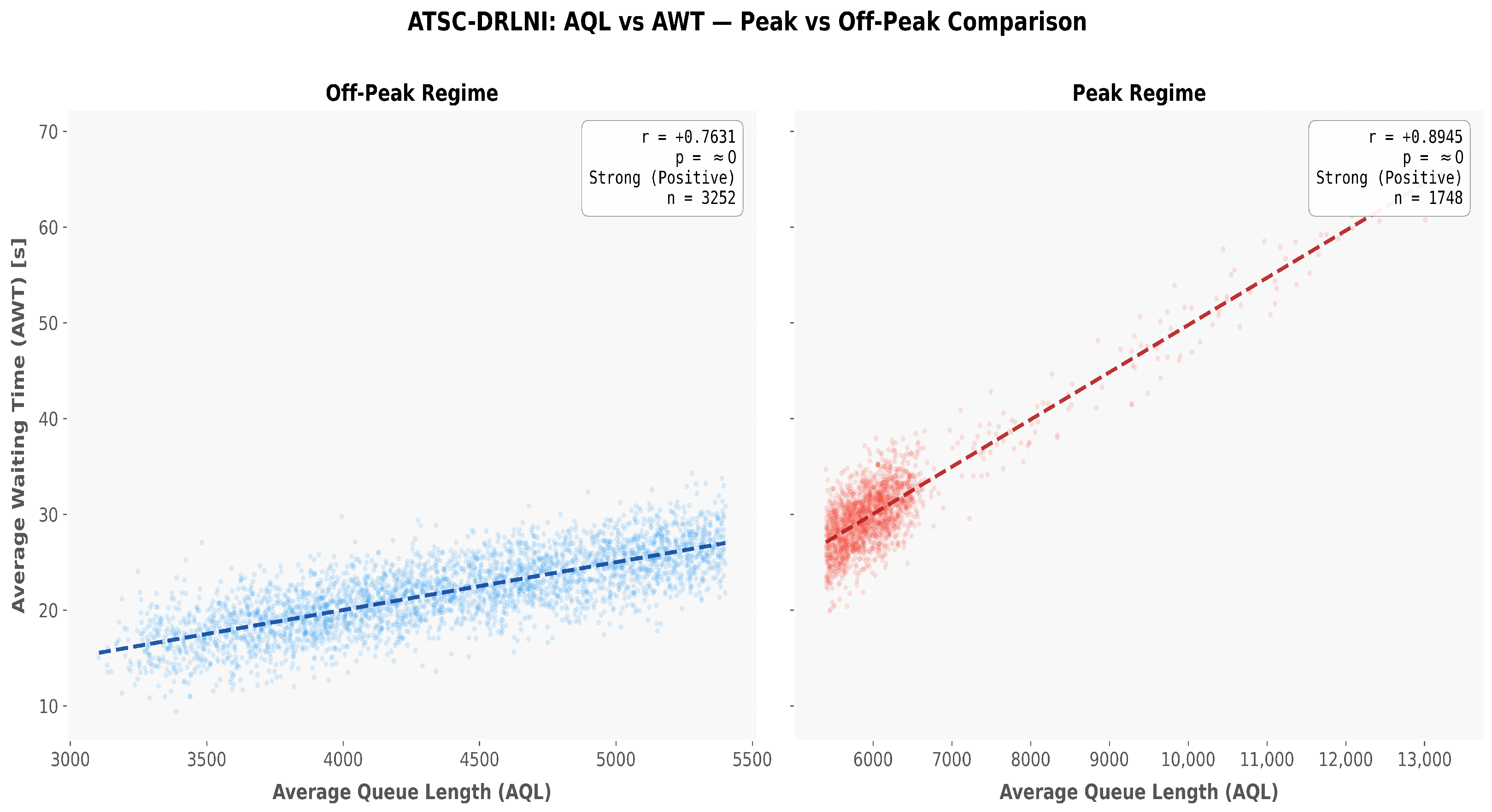
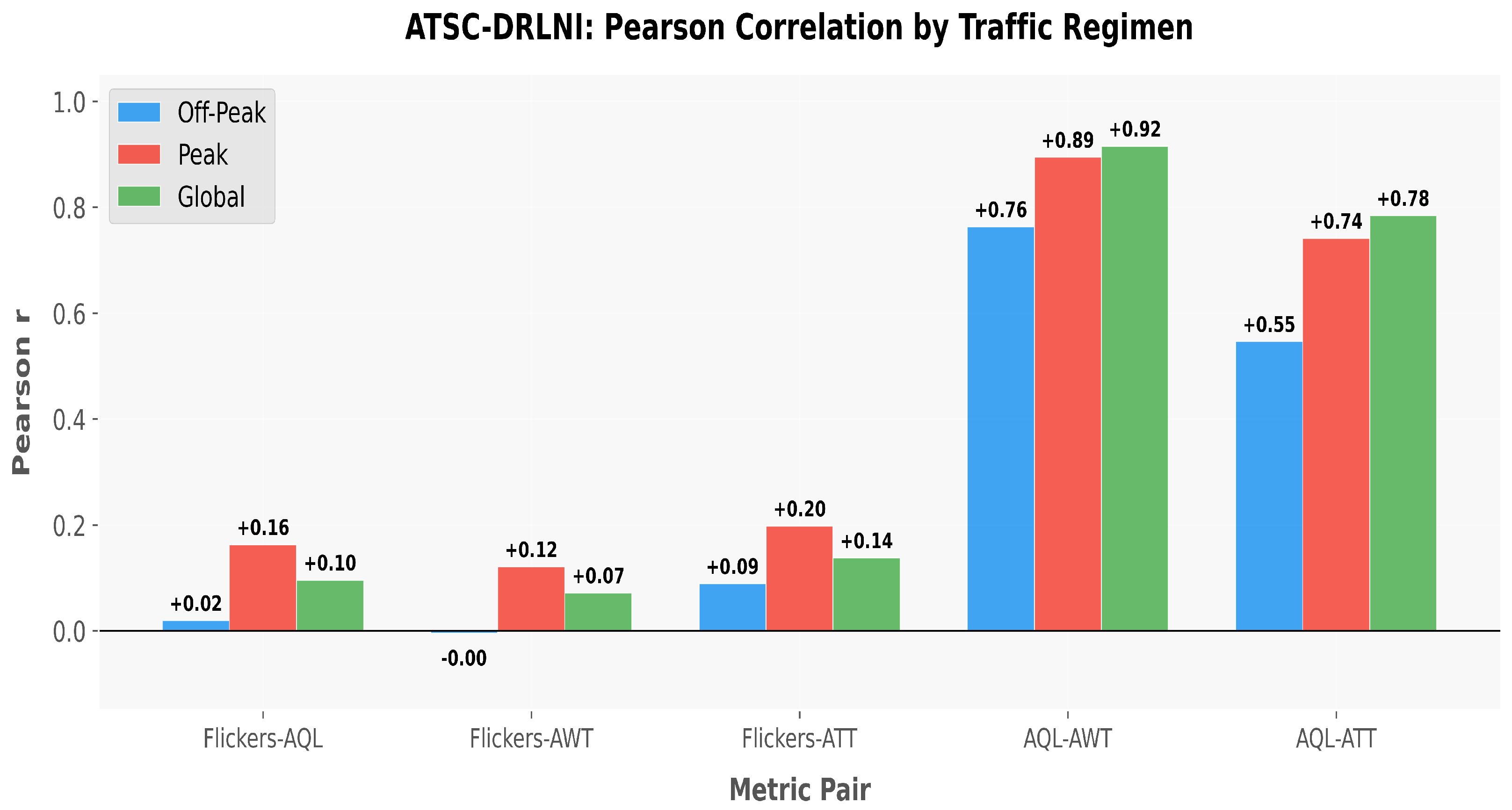
Based on this criterion, 3252 episodes ($65\%$) were classified as off-peak, with a mean AQL of 4376, while 1748 episodes ($35\%$) were classified as peak, with a mean AQL of 6146, which, as mentioned, were obtained from simulations of environments 2 and 3, shown in Figure 4. Table 10 presents the correlation results for both traffic regimes, along with the global correlations reported in Table 9 and the corresponding differences between off-peak and peak cases. Figure 12 illustrates the dispersion of AQL versus AWT under both traffic conditions, while Figure 13 summarizes the Pearson correlation coefficients for the five metric pairs analyzed.

4.4.3. Discussion of Pearson Correlation Coefficients by Traffic Regimen

Flickers versus AQL, AWT, and ATT. For off-peak episodes, the three correlations are very weak ($r\le +0.09$), whereas for peak episodes, the values increase slightly but remain weak ($r\le +0.20$). These results indicate a practical independence between flicker events and congestion-related metrics, confirming that penalizing flickers within the ATSC-DRLNI reward function does not adversely affect user-oriented performance indicators in either traffic regime.

AQL versus AWT. The Pearson correlation, classified as strong for off-peak episodes ($r=+0.76$), increases to very strong for peak episodes ($r=+0.89$), approaching a near-linear relationship under high-demand conditions. This behavior supports the internal coherence of the ATSC-DRLNI model across traffic regimes and is particularly relevant during peak periods, where congestion effects are more pronounced.

AQL versus ATT. For this pair, the Pearson correlations are strong in both regimes ($r=+0.55$ and $r=+0.74$, respectively), exhibiting the largest difference between off-peak and peak episodes ($\Delta r=+0.20$). Despite this variation, the results remain consistent across traffic conditions, reinforcing the stability of the learned relationships among operational metrics.

Notably, Pearson correlation coefficients are consistently higher for peak episodes ($\Delta r>0$ across the five metric pairs), indicating that the structural relationships among performance metrics become more pronounced under high-demand conditions. This behavior confirms that the ATSC-DRLNI model remains internally consistent across traffic regimes while preserving its operational properties.

1.

Robust decoupling: Correlation flickers versus AQL, AWT, and ATT are weak even in the peak episodes ($r<0.20$).

2.

Theoretical consistence: The increase in AQL–AWT/ATT correlation coefficient in peak episodes is consistent with Little’s law [77] and congestion propagation principles.

3.

Differential efficiency: The largest increase in AQL–ATT ($\Delta r=+0.20$) implies that the ATSC-DRLNI model has more impact, which is more important from a traffic control perspective, i.e., in congestion.

Overall, the advantages of ATSC-DRLNI are more evident during peak episodes, where stronger correlations among key operational metrics reflect stable and coherent behavior under congestion. Importantly, this improvement does not imply any deterioration in off-peak performance, demonstrating that the model maintains stability and efficiency simultaneously across varying traffic conditions.

5. Discussion and Limitations

Findings show a consistent positive correlation between the waiting time and the size of the queue length, similar to that shown in other studies [53,55], indicating that the inclusion of only one of two variables in the reward function is correct. The use of the number of flickers in the reward function showed a positive overall impact in the obtained results, in contrast to other methods for single intersections [47,48,49,53] where the reward function focuses only on waiting time and/or queue length without considering this variable.

The results presented suggest that optimization using the ATSC-DRLNI model can be a viable option to handle traffic lights and alleviate traffic congestion in real scenarios. From a theoretical point of view, results also align with those in [53,54,55,56,57], as our simulation results indicate the convenience of using a combined reward function in single intersections.

There is research that has also used flickers [53,55] in a DRL context with multi-objective models, showing reductions up to 18% in waiting time. However, these studies do not combine queue length and flickers in the reward function.

The good performance of the ATSC-DRLNI model in balancing traffic (Figure 9) and in queue reduction (Figure 6) are a direct consequence of the NI layer, which, by introducing controlled disturbances during training, forces agents to discriminate between spurious fluctuations in demand and real tendencies in congestion. This, in turn, prevents “over-reactions” in the control policy to small queue increments, a behavior that in other models (such as standard DQN) produces unstable phase changes. System stability, as shown in Figure 10, corroborates that agents have learned a more robust control policy that avoids overfitting with the data training set.

Although the ATSC-DRLNI framework does not explicitly implement a formal multi-objective optimization scheme, the correlation analysis across global, off-peak, and peak regimes indicates that stability-related and efficiency-related objectives do not exhibit structural conflict within the learned policy. The weak correlations between flickers and congestion metrics, together with the strong and consistent relationships among efficiency indicators, suggest that penalizing flickers does not compromise operational performance.

Nevertheless, an explicit multi-objective reinforcement learning (MORL) formulation could be explored in future work to formally characterize potential objective interactions under more heterogeneous traffic conditions or expanded state representations.

Beyond this conceptual consideration, the ATSC-DRLNI model presents several practical limitations. First, simulation times are longer compared to the other benchmark models evaluated. Second, certain environmental factors—such as pedestrians, priority vehicles (e.g., ambulances or police cars), and autonomous vehicles—were not included due to data and modeling constraints. Third, the current evaluation focuses on a single intersection, and more complex multi-intersection scenarios remain to be analyzed.

Future research should therefore address large-scale urban networks, modeling each intersection as a decentralized agent within a multi-agent deep reinforcement learning (MADRL) framework [78,79]. In addition, field testing will be necessary to assess the real-world applicability and robustness of the proposed ATSC strategy [31,47,78].

6. Conclusions

This research investigates the application of DRL to optimize ATSC and emphasizes the trade-off between minimizing queue lengths and suppressing signal instability at complex intersections. We developed and simulated a training environment on the SUMO platform, allowing the proposed ATSC-DRLNI model to learn signal timing policies through an A2C framework. Experimental results suggest that the agent skillfully balances queue size and phase flickers, outperforming seven benchmarks—including multi-agent approaches such as MADRL and MARDDPG—with a 40% reduction in queue length and sustained stability. However, although these results highlight the considerable potential of decentralized traffic management, they are limited to the simulated contexts described here.

A key contribution of this study is the analysis of how the A2C algorithm improves communication between agents and learning stability, enabling simultaneous optimization of queue lengths and signal flashes under congested traffic conditions. However, the disparity between the optimizations derived from simulation and practical implementation remains a major obstacle, especially with regard to physical constraints and unmodeled stochastic elements. To address this disparity, future research focused on validating these control strategies in increasingly realistic simulations or hardware-in-the-loop (HIL) is needed.

In addition, the methodology proposed in this paper could bridge the gap between theoretical autonomous traffic systems and their practical implementation, although it requires rigorous safety evaluations before real-world deployment. The proposed reward structure enables a balanced integration of efficiency-related metrics (AQL, AWT, ATT) and flickers, achieving consistent performance across off-peak and peak traffic regimen. Although DRL is widely studied in traffic control, translating these models into real-world settings remains challenging due to data constraints, safety requirements, and operational complexity. By grounding both training and validation in empirical traffic data, this framework contributes to narrowing the gap between simulation-based advances and practical implementation. Future work will explore explicit multi-objective reward formulations, the incorporation of vulnerable road users and emergency vehicles into the state representation, and extensions toward multi-intersection settings. Overall, these findings reinforce the practical potential of DRL as a scalable strategy for advancing adaptive traffic control systems (ATCSs) toward real-world deployment.

References

1. Thomson, I.; Bull, A. Urban traffic congestion: Its economic and social causes and consequences. Cepal Rev. 2006, 2002, 105–116. [Google Scholar] [CrossRef]
2. Bull, A.; United Nations; Economic Commission for Latin America and the Caribbean; Deutsche Gesellschaft für Technische Zusammenarbeit. Traffic Congestion: The Problem and How to Deal with It; Cuadernos de la CEPAL, United Nations, Economic Commission for Latin America and the Caribbean: Santiago, Chile, 2003. [Google Scholar]
3. González-Aliste, P.; Derpich, I.; López, M. Reducing Urban Traffic Congestion via Charging Price. Sustainability 2023, 15, 2086. [Google Scholar] [CrossRef]
4. Herath Bandara, S.J.; Thilakarathne, N. Economic and Public Health Impacts of Transportation-Driven Air Pollution in South Asia. Sustainability 2025, 17, 2306. [Google Scholar] [CrossRef]
5. Krzyzanowski, M.; Kuna-Dibbert, B.; Schneider, J. Health Effects of Transport-Related Air Pollution; WHO Regional Office Europe: Copenhagen, Denmark, 2005. [Google Scholar]
6. Zhang, K.; Batterman, S. Air pollution and health risks due to vehicle traffic. Sci. Total. Environ. 2013, 450–451, 307–316. [Google Scholar] [CrossRef]
7. INRIX. 2025 INRIX Global Traffic Scorecard; INRIX: Bellevue, WA, USA, 2025; Available online: https://inrix.com/scorecard/ (accessed on 14 February 2026).
8. Cravioto, J.; Yamasue, E.; Okumura, H.; Ishihara, K.N. Road transport externalities in Mexico: Estimates and international comparisons. Transp. Policy 2013, 30, 63–76. [Google Scholar] [CrossRef]
9. Salazar-Carrillo, J.; Torres-Ruiz, M.; Davis, C.A.; Quintero, R.; Moreno-Ibarra, M.; Guzmán, G. Traffic Congestion Analysis Based on a Web-GIS and Data Mining of Traffic Events from Twitter. Sensors 2021, 21, 2964. [Google Scholar] [CrossRef] [PubMed]
10. Thorne, E.; Chong Ling, E.; Phillips, W. Assessment of the Economic Costs of Vehicle Traffic Congestion in the Caribbean: A Case Study of Trinidad and Tobago; Technical Report; Naciones Unidas Comisión Económica para América Latina y el Caribe (CEPAL): Santiago, Chile, 2024. [Google Scholar]
11. Fleming, S. Traffic Congestion Cost the US Economy Nearly $87 Billion in 2018. World Economic Forum, 2019. Available online: https://www.weforum.org/stories/2019/03/traffic-congestion-cost-the-us-economy-nearly-87-billion-in-2018/ (accessed on 1 March 2026).
12. Pop, M.D.; Pandey, J.; Ramasamy, V. Future Networks 2030: Challenges in Intelligent Transportation Systems. In Proceedings of the 2020 8th International Conference on Reliability, Infocom Technologies and Optimization (Trends and Future Directions) (ICRITO), Noida, India, 4–5 June 2020; pp. 898–902. [Google Scholar] [CrossRef]
13. Goetz, A.R. Transport challenges in rapidly growing cities: Is there a magic bullet? Transp. Rev. 2019, 39, 701–705. [Google Scholar] [CrossRef]
14. Congestion, M.U.T. Managing Urban Traffic Congestion; OECD Publishing: Paris, France, 2007. [Google Scholar]
15. Eom, M.; Kim, B.I. The traffic signal control problem for intersections: A review. Eur. Transp. Res. Rev. 2020, 12, 50. [Google Scholar] [CrossRef]
16. Thunig, T.; Scheffler, R.; Strehler, M.; Nagel, K. Optimization and simulation of fixed-time traffic signal control in real-world applications. Procedia Comput. Sci. 2019, 151, 826–833. [Google Scholar] [CrossRef]
17. Koonce, P.; Rodegerdts, L. Traffic Signal Timing Manual; Technical Report; Federal Highway Administration: Washington, DC, USA, 2008. [Google Scholar]
18. Qadri, S.S.S.M.; Gökçe, M.A.; Öner, E. State-of-art review of traffic signal control methods: Challenges and opportunities. Eur. Transp. Res. Rev. 2020, 12, 55. [Google Scholar] [CrossRef]
19. Serban, A.A.; Frunzete, M. Analysis and comparison between urban traffic control systems. In Proceedings of the 2022 IEEE 28th International Symposium for Design and Technology in Electronic Packaging (SIITME), Bucharest, Romania, 26–29 October 2022; pp. 92–95. [Google Scholar] [CrossRef]
20. Cools, S.B.; Gershenson, C.; D’Hooghe, B. Self-Organizing Traffic Lights: A Realistic Simulation. In Advances in Applied Self-Organizing Systems; Springer: London, UK, 2013; pp. 45–55. [Google Scholar] [CrossRef]
21. Cools, S.B.; Gershenson, C.; D’Hooghe, B. Self-Organizing Traffic Lights: A Realistic Simulation. In Advanced Information and Knowledge Processing; Springer: Berlin/Heidelberg, Germany, 2008; pp. 41–50. [Google Scholar] [CrossRef]
22. Ferreira, M.; Fernandes, R.; Conceição, H.; Viriyasitavat, W.; Tonguz, O.K. Self-organized traffic control. In Proceedings of the Seventh ACM International Workshop on VehiculAr InterNETworking, VANET ’10, New York, NY, USA, 24 September 2010; pp. 85–90. [Google Scholar] [CrossRef]
23. Mirchandani, P.; Wang, F.Y. RHODES to intelligent transportation systems. IEEE Intell. Syst. 2005, 20, 10–15. [Google Scholar] [CrossRef]
24. Lowrie, P. SCATS, Sydney Co-Ordinated Adaptive Traffic System: A Traffic Responsive Method of Controlling Urban Traffic; Roads and Traffic Authority of New South Wales, Traffic Control Section: Darlinghurst, NSW, Australia, 1990. [Google Scholar]
25. Wang, T.; Cao, J.; Hussain, A. Adaptive Traffic Signal Control for large-scale scenario with Cooperative Group-based Multi-agent reinforcement learning. Transp. Res. Part Emerg. Technol. 2021, 125, 103046. [Google Scholar] [CrossRef]
26. Tunc, I.; Yesilyurt, A.Y.; Soylemez, M.T. Different Fuzzy Logic Control Strategies for Traffic Signal Timing Control with State Inputs. IFAC-PapersOnLine 2021, 54, 265–270. [Google Scholar] [CrossRef]
27. Shaikh, P.W.; El-Abd, M.; Khanafer, M.; Gao, K. A Review on Swarm Intelligence and Evolutionary Algorithms for Solving the Traffic Signal Control Problem. IEEE Trans. Intell. Transp. Syst. 2022, 23, 48–63. [Google Scholar] [CrossRef]
28. Guo, Y.; Liu, Y.; Oerlemans, A.; Lao, S.; Wu, S.; Lew, M.S. Deep learning for visual understanding: A review. Neurocomputing 2016, 187, 27–48. [Google Scholar] [CrossRef]
29. Kumar, R.; Sharma, N.V.K.; Chaurasiya, V.K. Adaptive traffic light control using deep reinforcement learning technique. Multimed. Tools Appl. 2024, 83, 13851–13872. [Google Scholar] [CrossRef]
30. Bálint, K.; Tamás, T.; Tamás, B. Deep Reinforcement Learning based approach for Traffic Signal Control. Transp. Res. Procedia 2022, 62, 278–285. [Google Scholar] [CrossRef]
31. Tan, J.; Yuan, Q.; Guo, W.; Xie, N.; Liu, F.; Wei, J.; Zhang, X. Deep Reinforcement Learning for Traffic Signal Control Model and Adaptation Study. Sensors 2022, 22, 8732. [Google Scholar] [CrossRef]
32. Damadam, S.; Zourbakhsh, M.; Javidan, R.; Faroughi, A. An Intelligent IoT Based Traffic Light Management System: Deep Reinforcement Learning. Smart Cities 2022, 5, 1293–1311. [Google Scholar] [CrossRef]
33. Ibrokhimov, B.; Kim, Y.J.; Kang, S. Biased Pressure: Cyclic Reinforcement Learning Model for Intelligent Traffic Signal Control. Sensors 2022, 22, 2818. [Google Scholar] [CrossRef] [PubMed]
34. Wu, J.; Ran, Y.; Lou, Y.; Shu, L. CenLight: Centralized traffic grid signal optimization via action and state decomposition. IET Intell. Transp. Syst. 2023, 17, 1247–1261. [Google Scholar] [CrossRef]
35. Abdelghaffar, H.M.; Rakha, H.A. A Novel Decentralized Game-Theoretic Adaptive Traffic Signal Controller: Large-Scale Testing. Sensors 2019, 19, 2282. [Google Scholar] [CrossRef]
36. Mo, Z.; Li, W.; Fu, Y.; Ruan, K.; Di, X. CVLight: Decentralized learning for adaptive traffic signal control with connected vehicles. Transp. Res. Part Emerg. Technol. 2022, 141, 103728. [Google Scholar] [CrossRef]
37. Chow, A.H.; Sha, R.; Li, S. Centralised and decentralised signal timing optimisation approaches for network traffic control. Transp. Res. Part Emerg. Technol. 2020, 113, 108–123. [Google Scholar] [CrossRef]
38. Guo, Q.; Li, L.; Jeff Ban, X. Urban traffic signal control with connected and automated vehicles: A survey. Transp. Res. Part Emerg. Technol. 2019, 101, 313–334. [Google Scholar] [CrossRef]
39. Chu, T.; Wang, J.; Codeca, L.; Li, Z. Multi-agent deep reinforcement learning for large-scale traffic signal control. IEEE Trans. Intell. Transp. Syst. 2020, 21, 1086–1095. [Google Scholar] [CrossRef]
40. Zhao, H.; Dong, C.; Cao, J.; Chen, Q. A survey on deep reinforcement learning approaches for traffic signal control. Eng. Appl. Artif. Intell. 2024, 133, 108100. [Google Scholar] [CrossRef]
41. Aoki, S.; Rajkumar, R. Cyber Traffic Light: Safe Cooperation for Autonomous Vehicles at Dynamic Intersections. IEEE Trans. Intell. Transp. Syst. 2022, 23, 22519–22534. [Google Scholar] [CrossRef]
42. Wang, B.; He, Z.; Sheng, J.; Chen, Y. Deep Reinforcement Learning for Traffic Light Timing Optimization. Processes 2022, 10, 2458. [Google Scholar] [CrossRef]
43. El-Qoraychy, F.Z.; Dridi, M.; Creput, J.C. Deep Reinforcement Learning for Vehicle Intersection Management in High-Dimensional Action Spaces. In Proceedings of the 2024 7th International Conference on Machine Learning and Machine Intelligence (MLMI), MLMI ’24, New York, NY, USA, 2–4 August 2024; pp. 39–45. [Google Scholar] [CrossRef]
44. Shi, Y.; Wang, Z.; LaClair, T.J.; Wang, C.R.; Shao, Y.; Yuan, J. A Novel Deep Reinforcement Learning Approach to Traffic Signal Control with Connected Vehicles. Appl. Sci. 2023, 13, 2750. [Google Scholar] [CrossRef]
45. Miletić, M.; Ivanjko, E.; Gregurić, M.; Kušić, K. A review of reinforcement learning applications in adaptive traffic signal control. IET Intell. Transp. Syst. 2022, 16, 1269–1285. [Google Scholar] [CrossRef]
46. Majstorović, Ž.; Tišljarić, L.; Ivanjko, E.; Carić, T. Urban Traffic Signal Control under Mixed Traffic Flows: Literature Review. Appl. Sci. 2023, 13, 4484. [Google Scholar] [CrossRef]
47. Zhong, D.; Boukerche, A. Traffic Signal Control Using Deep Reinforcement Learning with Multiple Resources of Rewards. In Proceedings of the 16th ACM International Symposium on Performance Evaluation of Wireless Ad Hoc, Sensor, & Ubiquitous Networks, PE-WASUN ’19, New York, NY, USA, 25–29 November 2019; pp. 23–28. [Google Scholar] [CrossRef]
48. Li, D.; Wu, J.; Xu, M.; Wang, Z.; Hu, K. Adaptive Traffic Signal Control Model on Intersections Based on Deep Reinforcement Learning. J. Adv. Transp. 2020, 2020, 6505893. [Google Scholar] [CrossRef]
49. Pan, T. Traffic Light Control with Reinforcement Learning. arXiv 2023, arXiv:2308.14295. [Google Scholar] [CrossRef]
50. Agrawal, A.; Paulus, R. Intelligent traffic light design and control in smart cities: A survey on techniques and methodologies. Int. J. Veh. Inf. Commun. Syst. 2020, 5, 436–481. [Google Scholar] [CrossRef]
51. Li, Z.; Xu, C.; Zhang, G. A Deep Reinforcement Learning Approach for Traffic Signal Control Optimization. arXiv 2021, arXiv:2107.06115. [Google Scholar] [CrossRef]
52. Nawar, M.; Fares, A.; Al-Sammak, A. Rainbow Deep Reinforcement Learning Agent for Improved Solution of the Traffic Congestion. In Proceedings of the 2019 7th International Japan-Africa Conference on Electronics, Communications, and Computations, (JAC-ECC), Alexandria, Egypt, 15–16 December 2019; pp. 80–83. [Google Scholar] [CrossRef]
53. Mirbakhsh, S.; Azizi, M. Adaptive traffic signal safety and efficiency improvement by multi objective deep reinforcement learning approach. arXiv 2024, arXiv:2408.00814. [Google Scholar] [CrossRef]
54. Shao, J.; Zheng, C.; Chen, Y.; Huang, Y.; Zhang, R. MoveLight: Enhancing Traffic Signal Control through Movement-Centric Deep Reinforcement Learning. arXiv 2024, arXiv:2407.17303. [Google Scholar] [CrossRef]
55. Sattarzadeh, A.R.; Pathirana, P.N. Enhancing Adaptive Traffic Control Systems with Deep Reinforcement Learning and Graphical Models. In Proceedings of the 2024 IEEE International Conference on Future Machine Learning and Data Science (FMLDS), Sydney, NSW, Australia, 20–23 November 2024; pp. 39–44. [Google Scholar] [CrossRef]
56. Dhashyanth, N.; Hemchand, R.; Priyanga, R.; Soorya, S.; Sudheesh, P. Adaptive Traffic Control Using Deep Reinforcement Learning. In Proceedings of the 2024 IEEE Pune Section International Conference (PuneCon), Pune, India, 13–15 December 2024; pp. 1–8. [Google Scholar] [CrossRef]
57. Ma, D.; Zhou, B.; Song, X.; Dai, H. A Deep Reinforcement Learning Approach to Traffic Signal Control With Temporal Traffic Pattern Mining. IEEE Trans. Intell. Transp. Syst. 2022, 23, 11789–11800. [Google Scholar] [CrossRef]
58. Lecun, Y.; Bottou, L.; Bengio, Y.; Haffner, P. Gradient-based learning applied to document recognition. Proc. IEEE 1998, 86, 2278–2324. [Google Scholar] [CrossRef]
59. Zhang, A.; Lipton, Z.C.; Li, M.; Smola, A.J. Dive into Deep Learning; Cambridge University Press: Cambridge, UK, 2023; Available online: https://D2L.ai (accessed on 1 March 2026).
60. Abiodun, O.I.; Jantan, A.; Omolara, A.E.; Dada, K.V.; Mohamed, N.A.; Arshad, H. State-of-the-art in artificial neural network applications: A survey. Heliyon 2018, 4, e00938. [Google Scholar] [CrossRef]
61. Goodfellow, I.; Bengio, Y.; Courville, A. Deep Learning; MIT Press: Cambridge, MA, USA, 2016; Available online: http://www.deeplearningbook.org (accessed on 1 March 2026).
62. François-Lavet, V.; Henderson, P.; Islam, R.; Bellemare, M.G.; Pineau, J. An introduction to deep reinforcement learning. Found. Trends Mach. Learn. 2018, 11, 219–354. [Google Scholar] [CrossRef]
63. Nian, R.; Liu, J.; Huang, B. A review On reinforcement learning: Introduction and applications in industrial process control. Comput. Chem. Eng. 2020, 139, 106886. [Google Scholar] [CrossRef]
64. Mahadevan, S. Average reward reinforcement learning: Foundations, algorithms, and empirical results. Mach. Learn. 1996, 22, 159–195. [Google Scholar] [CrossRef]
65. Naeem, M.; Rizvi, S.T.H.; Coronato, A. A Gentle Introduction to Reinforcement Learning and its Application in Different Fields. IEEE Access 2020, 8, 209320–209344. [Google Scholar] [CrossRef]
66. Aubret, A.; Matignon, L.; Hassas, S. An Information-Theoretic Perspective on Intrinsic Motivation in Reinforcement Learning: A Survey. Entropy 2023, 25, 327. [Google Scholar] [CrossRef]
67. Hariharan, N.; Anand, P.G. A Brief Study of Deep Reinforcement Learning with Epsilon-Greedy Exploration. Int. J. Comput. Digit. Syst. 2022, 11, 541–551. [Google Scholar] [CrossRef]
68. Dabney, W.; Ostrovski, G.; Barreto, A. Temporally-Extended ε-Greedy Exploration. In Proceedings of the International Conference on Learning Representations, Online, 3–7 May 2021. [Google Scholar] [CrossRef]
69. Konda, V.; Tsitsiklis, J. Actor-Critic Algorithms. In Proceedings of the Advances in Neural Information Processing Systems; Solla, S., Leen, T., Müller, K., Eds.; MIT Press: Cambridge, MA, USA, 1999; Volume 12. [Google Scholar] [CrossRef]
70. Grondman, I.; Busoniu, L.; Lopes, G.A.D.; Babuška, R. A survey of actor-critic reinforcement learning: Standard and natural policy gradients. IEEE Trans. Syst. Man Cybern. Part Appl. Rev. 2012, 42, 1291–1307. [Google Scholar] [CrossRef]
71. Wang, K.; Liu, A.; Lin, B. Single-Loop Deep Actor-Critic for Constrained Reinforcement Learning With Provable Convergence. IEEE Trans. Signal Process. 2024, 72, 4871–4887. [Google Scholar] [CrossRef]
72. Zur, R.M.; Jiang, Y.; Pesce, L.L.; Drukker, K. Noise injection for training artificial neural networks: A comparison with weight decay and early stopping. Med. Phys. 2009, 36, 4810–4818. [Google Scholar] [CrossRef]
73. Bishop, C.M. Training with Noise is Equivalent to Tikhonov Regularization. Neural Comput. 1995, 7, 108–116. [Google Scholar] [CrossRef]
74. Fujimoto, S.; Hoof, H.; Meger, D. Addressing function approximation error in actor-critic methods. In Proceedings of the International Conference on Machine Learning, PMLR, Stockholm, Sweden, 10–15 July 2018; pp. 1587–1596. [Google Scholar]
75. Camuto, A.; Willetts, M.; Simsekli, U.; Roberts, S.J.; Holmes, C.C. Explicit Regularisation in Gaussian Noise Injections. In Proceedings of the Advances in Neural Information Processing Systems; Larochelle, H., Ranzato, M., Hadsell, R., Balcan, M., Lin, H., Eds.; Curran Associates, Inc.: Red Hook, NY, USA, 2020; Volume 33, pp. 16603–16614. [Google Scholar]
76. Evans, J.D. Straightforward Statistics for the Behavioral Sciences; Thomson Brooks/Cole Publishing Co.: Pacific Grove, CA, USA, 1996. [Google Scholar]
77. Little, J.D.; Graves, S.C. Little’s law. In Building Intuition: Insights from Basic Operations Management Models and Principles; Springer: New York, NY, USA, 2008; pp. 81–100. [Google Scholar]
78. Yang, T.; Fan, W. Enhancing Robustness of Deep Reinforcement Learning Based Adaptive Traffic Signal Controllers in Mixed Traffic Environments Through Data Fusion and Multi-Discrete Actions. IEEE Trans. Intell. Transp. Syst. 2024, 25, 14196–14208. [Google Scholar] [CrossRef]
79. Friesen, M.; Tan, T.; Jasperneite, J.; Wang, J. Application of Multi-Agent Deep Reinforcement Learning to Optimize Real-World Traffic Signal Controls. Authorea Prepr. 2021. [Google Scholar] [CrossRef]
Figure 1. Proposed decentralized DRL framework (ATSC-DRLNI) architecture with 4 convolutional neural networks (CNNs), a noise injection (NI) layer, and three output layers.
Applsci 16 03833 g001
Figure 2. Data flow in the CNN structure in the ATSC-DRLNI model.
Applsci 16 03833 g002
Figure 3. Intersection used for training of ATSC-DRLNI. The red central area is the intersection between the black streets, composed by street lanes separated by white dashed lines. In the central area, red and gray lines represent the valid lane changes. The small red dots represent the traffic sensors.
Applsci 16 03833 g003
Figure 4. Two intersections used to test ATSC-DRLNI model. The central area of the two zoomed intersections between the black streets are composed by street lanes separated by white dashed lines.
Applsci 16 03833 g004
Figure 5. Simulation training results: Average Reward (AR). The lines use a rolling mean with a window of 10 episodes. The shaded area is the standard deviation. The markers are the sampling points, and the big circles are the best observed values.
Applsci 16 03833 g005
Figure 6. Simulation training results: Average Queue Length (AQL). The lines use a rolling mean with a window of 10 episodes. The shaded area is the standard deviation. The markers are the sampling points, and the big circles are the best observed values.
Applsci 16 03833 g006
Figure 7. Simulation training results: adimensional number of traffic light changes (flicker). The lines use a rolling mean with a window of 10 episodes. The shaded area is the standard deviation. The markers are the sampling points, and the big circles are the best observed values.
Applsci 16 03833 g007
Figure 8. Learning stability comparison across of the 8 simulated methods after training.
Applsci 16 03833 g008
Figure 9. Traffic balance of the 8 simulated methods after training.
Applsci 16 03833 g009
Figure 10. System stability of the 8 simulated methods after training.
Applsci 16 03833 g010
Figure 11. Sensitivity analysis of the variance hyperparameter ( σ 2 ) on the average tail length (AQL) and phase flicker rate.
Applsci 16 03833 g011
Figure 12. ATSC-DRLNI model data dispersion for AQL versus AWT Pearson correlation by traffic regimen. Correlation increases from r = + 0.76 for off-peak traffic episodes to r = + 0.89 for peak traffic episodes.
Applsci 16 03833 g012
Figure 13. Comparison of ATSC-DRLNI model Pearson correlation coefficients by traffic regimen.
Applsci 16 03833 g013