Design and Optimization of a Two-Tier Supply Chain Network Under Demand Uncertainty Using Genetic Algorithm and Particle Swarm Optimization

Featured Application

The proposed bi-level optimization framework can support decision-making in decentralized supply chains with multiple factories, retailers, and products under demand uncertainty. By capturing hierarchical interactions between production facilities and retailers, the model enables coordinated production, pricing, and allocation decisions, improving operational efficiency and overall profitability at both the production and retailer levels.

Abstract

Supply chain management (SCM) involves complex coordination among multiple actors under demand uncertainty. However, most existing studies focus on simplified network structures that fail to capture all relevant dimensions of real-world supply chains or assume deterministic demand. This study proposes a comprehensive stochastic bi-level optimization framework for a multi-factory, multi-retailer, multi-customer, and multi-product supply chain network. The model captures the hierarchical interaction between decision-makers, where the production facility owner acts as the leader and the retailer as the follower, and jointly optimizes profit across both levels. To efficiently solve the resulting bi-level problem, two tailored metaheuristic solution approaches—a two-tier genetic algorithm (TT-GA) and a two-tier particle swarm optimization (TT-PSO)—are developed. Computational experiments across multiple scenarios demonstrate that TT-PSO outperforms TT-GA in Scenarios 1 and 2, achieving overall profit improvements of 6.46% and 0.76%, respectively, while TT-GA yields superior performance in Scenario 3 with a 2.80% profit improvement. The proposed framework provides decision-makers with a robust and practical tool for improving profitability and operational efficiency in complex, uncertain supply chain environments.

1. Introduction

From the origin of raw materials all the way to the consumer’s hands, supply chains are sophisticated systems that have an important role in many aspects of our lives. Numerous facilities and tasks are required for creating, distributing, and delivering goods to meet consumer demands that naturally have some uncertainty. Coordination and cooperation at all levels of the supply chain are key elements for efficient management to keep production, inventory, and distribution costs at a minimum and boost profitability. Decision-makers must integrate supply chain strategies at every stage of the supply chain and make wise choices to accomplish this goal, which can be a challenge, especially when there are multiple players in the course of action.

The growing complexity of supply chain systems has led researchers to develop advanced analytical and optimization approaches to support decision-making processes in such environments. In particular, supply chain management has increasingly relied on quantitative models to coordinate production, inventory, and distribution decisions across multiple echelons of the network. These models help decision-makers evaluate the efficiency of cost, service level, and responsiveness while coping with uncertain demand and operational constraints. Prior studies have highlighted the importance of integrated decision-support frameworks for improving coordination among supply chain participants and enhancing overall system performance [1,2]. As supply chains continue to expand in scale and structural complexity, the need for modeling approaches that capture interactions among multiple actors and decision layers becomes even more critical.

Modern supply chains are multifaceted networks involving multiple actors, including suppliers, manufacturers, distributors, retailers, and end customers. These actors are often geographically dispersed across multinational business environments, which significantly increases the complexity of supply chain management. In decentralized supply chains, each decision-maker independently controls a specific set of decision variables and pursues individual objectives. However, because these decisions collectively affect overall supply chain performance, it is essential to explicitly account for the interactions and strategic behavior of multiple actors. Decentralized supply chains, with their greater adaptability and responsiveness to customer demand, have attracted increasing research attention.

The modeling of decentralized decision-making processes frequently relies on hierarchical and game-theoretic frameworks [3]. Bi-level programming provides a natural mathematical structure for representing strategic interactions between upper- and lower-level decision-makers, in which decisions are made sequentially in response to one another. Although several studies have applied bi-level optimization to decentralized supply chains, most existing works focus on simplified network structures that fail to capture all relevant dimensions of real-world supply chains and typically assume deterministic demand. This leaves a notable research gap in modeling more realistic, large-scale, multi-echelon supply chains under demand uncertainty.

To address the identified research gap, this study proposes a stochastic bi-level optimization framework for a multi-period, multi-factory, multi-retailer, multi-customer, and multi-product supply chain network under demand uncertainty. The proposed model captures hierarchical interactions in a leader–follower setting, where plant owners act as the leaders and retailers represent the followers, whose decisions are influenced by uncertain customer demand. The framework jointly determines optimal production, distribution, and allocation quantities at each echelon with the objective of maximizing total profit for both plants and retailers.

Given the nonlinear and large-scale nature of the resulting bi-level problem, two tailored metaheuristic solution approaches—a two-tier genetic algorithm (TT-GA) and a two-tier particle swarm optimization method (TT-PSO)—are developed to efficiently obtain high-quality solutions. A comparative analysis of these methods is conducted using three illustrative data sets to evaluate the effectiveness of the proposed framework and solution procedures. The results demonstrate the practical applicability of the model to realistic multi-dimensional supply chain settings and highlight its potential to improve profitability and operational efficiency in complex and uncertain supply chain environments.

The remainder of this work is organized as follows. Section 2 outlines the methods and materials employed in the study. Section 3 provides the problem description and presents the mathematical formulation. The proposed solution methodologies are elaborated on in Section 4. A case study demonstrating the application of the proposed framework is detailed in Section 5 with the associated results and discussions. Finally, Section 6 concludes the paper and suggests directions for future research.

2. Materials and Methods

In this section, we give an overview of bilevel programming and metaheuristics, demand uncertainty, and a comparison of notable related studies in the field.

2.1. Metaheuristics

Metaheuristic algorithms are commonly used in solving complex optimization problems to find an approximate solution in a relatively short time when compared to exact solution algorithms. They are used in many different types of NP-hard problems, including traveling salesperson (TSP) [4,5], knapsack [6,7], packing [8,9], and scheduling [10,11] problems. They are also efficiently used to solve bilevel optimization problems [12,13,14]. A range of metaheuristics, including evolutionary algorithms, swarm intelligence, tabu search, and annealing-based methods, are prevalent in tackling complex optimization problems. In this study, an evolutionary algorithm and a swarm intelligence approach are adopted to solve the developed bilevel model.

2.1.1. Genetic Algorithm (GA)

In 1975, John Holland first laid out GA, a prominent and effective meta-heuristic algorithm. It is a stochastic global search and optimization methodology inspired by natural selection and biological evolution, addressing difficult problems by imitating the evolutionary processes of nature across generations [15,16]. A genetic algorithm starts by creating a population of possible solutions to a problem at random. A fitness function assesses each solution to ascertain its efficacy. The method utilizes two primary operators: crossover, which amalgamates attributes of two parent solutions to generate new offspring, and mutation, which introduces minor random alterations to the offspring’s characteristics to formulate new solutions. The processes of selection, crossover, and mutation are carried out by a multitude of generations, which ultimately results in the gradual refinement of solutions. After that, the process will continue until it finds a solution that is either optimal or nearly optimal [17,18]. The algorithm is successfully used for complex optimization problems, as can be seen in recent studies in refs. [19,20].

2.1.2. Particle Swarm Optimization (PSO)

PSO, an algorithm developed by James Kennedy and Russell Eberhart, first appeared in 1995. PSO mimics the intelligent group behavior of animal swarms by allowing particles to communicate information about their environment in order to help the collective perform better as a whole [21,22]. Every particle in the PSO functions as a prospective solution to the optimization problem [23,24]. Every particle in the swarm possesses a position and velocity. The location signifies a prospective solution, while a collection of such solutions, referred to as particles, navigates the search space to identify the ideal solution. The velocity denotes the direction and speed of each particle’s motion inside the swarm. This optimization method is unique in that it relies solely on the objective function, without the need for gradients or differential forms, rendering it appropriate for non-differentiable situations. Moreover, it possesses a limited quantity of hyperparameters, hence streamlining the setting and mitigating the likelihood of overfitting. The program concludes when optimal conditions are satisfied, usually determined by a predetermined number of iterations or reaching a designated fitness threshold [25,26]. This adaptability enables PSO to address diverse optimization challenges, rendering it an effective instrument for resolving intricate real-world issues as done in refs. [27,28].

2.2. Bilevel Optimization

Dating back to the 1970s, bilevel optimization is a relatively new area of study that is used in hierarchical decision-making processes in which a leader acts first, then a follower [29]. The decision of the leader as the upper-level entity is affected by the response of the follower as the lower-level entity, with each side having its own objective and constraints [30]. The approach is efficiently used in many different areas, including project management in a competitive environment [31], analyzing the vulnerabilities in a network [32], maximizing hosting capacity of power systems [33], protection of healthcare networks [34], efficient traffic management [35], robust scheduling in high-precision manufacturing [36], and reorganizing medical consumable orders [37].

Finding an exact solution to bilevel optimization problems can be a challenge since they are known to be strongly NP-hard [38,39]. The complex nature of the problem makes it necessary to use a metaheuristic method for timely and efficient solutions. The recent literature shows a growing trend of integrating metaheuristic methods with bilevel programming frameworks. A bilevel optimization model for a rice supply chain, focusing on minimizing total costs from the perspectives of two distinct decision-makers, was developed in ref. [40]. The study employed two prominent metaheuristic methods, namely GA and PSO, to proficiently address the bilevel problem. Survey in ref. [41] investigated a decentralized production-distribution system comprising a single manufacturer and distributor, where market demand is jointly influenced by pricing and promotional strategies. It introduced two nonlinear bilevel programming models by alternating the leadership roles of the manufacturer and the distributor. The efficacy and efficiency of the proposed GA and PSO methods were evaluated and compared through comprehensive computational testing. The integration of retail contracts for product line design was analyzed in ref. [42]. Their approach was built on a co-evolutionary optimization framework that utilizes a nested hierarchical GA to analyze how different contractual structures and their specific terms influence final product specifications, pricing strategies, market distribution, and the profits of both parties involved. Similarly, refs. [43,44] have also employed bilevel optimization for sustainable supply chain network design, integrating environmental and social objectives into the core decision-making framework. A novel strategy to facilitate the adoption of cleaner technologies was presented in ref. [43], whereas ref. [44] concentrated on mitigating carbon emissions in transportation by assuring coordination in product distribution volumes to improve overall supply chain sustainability. Both pieces of research employed heuristic methodologies.

2.3. Demand Uncertainty

Demand uncertainty significantly impacts decision-making processes and operational strategies within the dynamic context of supply chain management. Neglecting demand uncertainty may result in overstocking, elevated holding costs, stockouts, lost sales, and diminished customer satisfaction. Ineffective resource distribution resulting from demand variability can increase total costs for supply chain entities. Consequently, effectively managing demand uncertainty is essential for optimizing inventory, production planning, distribution, and the overall performance of the supply chain. Numerous studies have been conducted over time to handle demand uncertainty in supply chain networks. A multi-objective design for hydrogen supply chain networks considering demand uncertainty was proposed in ref. [1]. The authors incorporated uncertainty by establishing lower and upper bounds for hydrogen demand, assessing the tolerance between these bounds. The study in ref. [45] examined uncertainty in demand as well as in returned products. Demand uncertainty was represented through a normal distribution, considering the mean and variance of the product. Under a scenario of demand uncertainty, ref. [46] studied the best way for a single manufacturer and their various suppliers to coordinate quantity discounts to optimize the supply chain. The study utilized a normal distribution model to account for demand uncertainty.

2.4. A Comparison of Related Studies

Research has focused on bilevel supply chains, examining strategies to manage demand uncertainty, optimize coordination, and improve efficiency among supply chain participants. Conceptually, this work extends the framework of ref. [47], which employed a two-stage stochastic program to address mid-term supply chain planning with demand uncertainty, multiple products, and distributed production sites. Extending this approach to uncertainty, foundational methods for the multiperiod planning and scheduling of facilities producing multiple products within a stochastic environment were developed by ref. [48]. Later, leveraging the methodological contributions of ref. [48], a multi-period bilevel model to manage demand uncertainty by reformulating the follower’s objective function was developed by ref. [49].

Shifting the focus to hierarchical coordination, ref. [50] analyzed a three-echelon supply chain under scenario-based stochastic demand. Their work, which also aligns with the Stackelberg game-theoretic perspective shared by ref. [49], specifically investigated the role of corporate social responsibility investments, casting the manufacturer in the leader role and the retailer as the follower. Similarly, ref. [46] developed a quantity discount strategy to improve the operational efficiency of the supply chain under fluctuating demand conditions. A solution approach was presented for a scenario involving one manufacturer and multiple suppliers offering various products. Consistent with prior research, a stochastic programming model was reformulated utilizing normalization techniques to address the uncertainty inherent in the demand. The comparison of the innovative studies in the field is summarized in

Table 1. Overview of the key literature.

Study	Research Problem	Structure of Modeling					Solution Method	Solution Algorithm	Uncertainty	Sources of Uncertainty
		Type of Model	Period		Product
			Single	Multi	Single	Multi
Robles et al. (2020) [3]	Production-Distribution	MO		✔	✔		ε-constraint Method, Metaheuristics	GA	✔	Demand
Cheraghali-pour et al. (2019) [40]	Production-Distribution	BP		✔		✔	Metaheuristics	GA, PSO
Amirtaheri et al. (2017) [41]	Production-Distribution	BP	✔		✔		Metaheuristics	GA, PSO
Kwong et al. (2021) [42]	Production Line Design	BP	✔			✔	Metaheuristics	GA
Chalmardi & Camacho (2019) [43]	Production-Distribution	BP	✔		✔		Heuristics	SA
Haque et al. (2020) [44]	Production-Distribution	BP		✔	✔		Heuristics
Cui et al. (2017) [45]	Remanufacturing	SO	✔		✔		Metaheuristics	ABC, GA, GABC	✔	Demand, Returned Products
Yin et al. (2015) [46]	Quantity Discounts	BP	✔			✔	Exact method		✔	Demand
Gupta et al. (2000) [47]	Production Planning	MO	✔			✔	Exact Method		✔	Demand
Nishi & Yoshida (2016) [49]	Production-Distribution	BP		✔		✔	Exact method		✔	Demand
Hosseini-Motlagh (2019) [50]	Wholesale Price Contract	BP	✔		✔		Exact Method		✔	Demand
Nezamoddini& Gholami (2019) [51]	Risk Analysis	SO		✔	✔		Metaheuristics, Artificial Neural Networks	GA	✔	Demand
Setak et al. (2019) [52]	Location, Pricing	BP	✔		✔		Exact method, Metaheuristics	GA	✔	Demand
This study, 2026	Production-Distribution	BP		✔		✔	Metaheuristics	GA, PSO	✔	Demand

Note: Single Objective Optimization (SO); Multi-Objective Optimization (MO); Bilevel Programming Optimization (BP); Genetic Algorithm (GA); Particle Swarm Optimization (PSO); Artificial Bee Colony Algorithm (ABC); Genetic Artificial Bee Colony Algorithm (GABC); Simulated Annealing (SA).

.

Table 1 presents the solution methods and algorithms used on the research problem in this study in comparison with other studies in the literature. This research presents, to the best of our knowledge, one of the first integrated stochastic bi-level optimization frameworks for the joint modeling and optimization of a multi-period, multi-product, multi-factory supply chain network under demand uncertainty. By focusing on two well-established metaheuristic approaches (TT-GA and TT-PSO) to demonstrate the effectiveness and robustness of the proposed framework in addressing this complex structure, the principal contributions of this work are summarized as follows:

• Develop a stochastic bi-level, multi-echelon supply chain model that captures hierarchical decision-making between plant owners (leaders) and retailers (followers) in a three-echelon network comprising plants, retailers, and customers across multiple products and periods.
• Incorporate demand uncertainty explicitly at the lower level of the bi-level model, enabling more realistic modeling of customer-driven decision-making in decentralized supply chains.
• Design and compare two tailored two-tier metaheuristic solution approaches (TT-GA and TT-PSO) to efficiently solve the resulting large-scale nonlinear bi-level problem, and evaluate their performance using three distinct data sets in terms of solution quality and total profit improvement.

3. Problem Description and Model Formulation

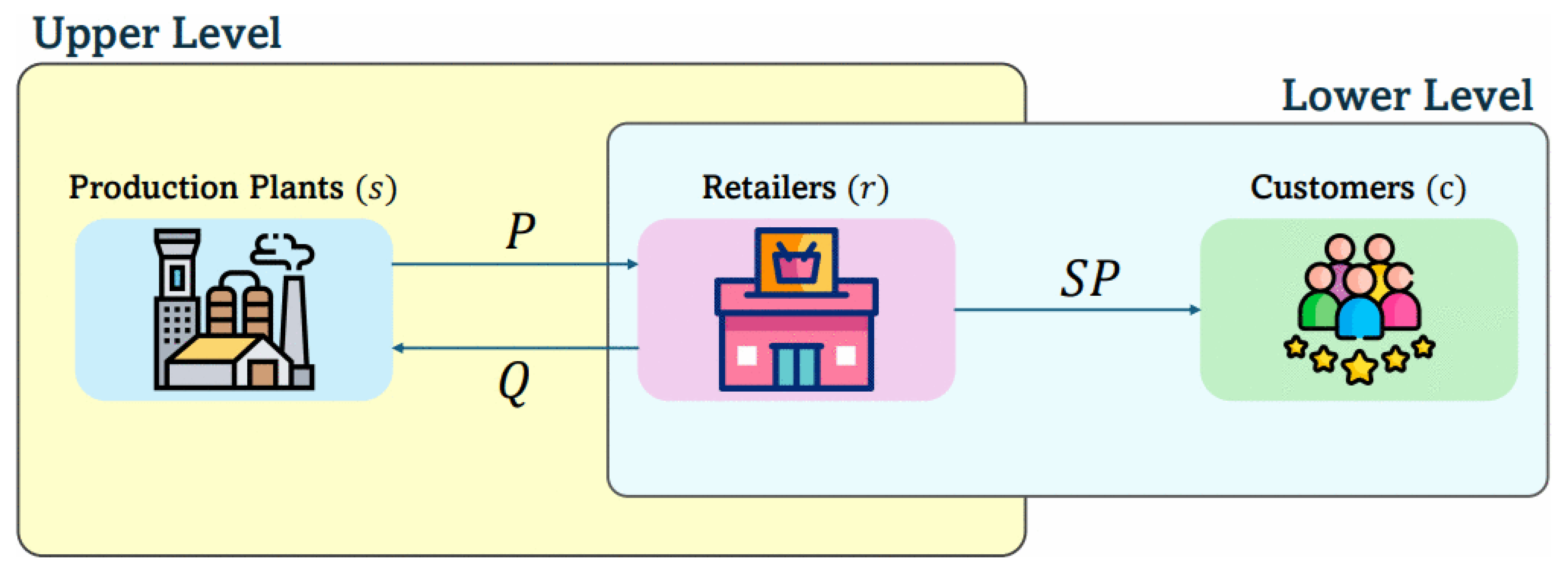
We design a two-tier supply chain network structured with three echelons as shown in Figure 1. The initial echelon comprises production facilities tasked with the fabrication of products. The second echelon consists of retailers that directly sell products to consumers. The third echelon consists of end customers who acquire and utilize the products. Note that, interacting with both production plants and customers, the retailer is at the intersection of both upper and lower levels of the chain and follows any decision at the production level. This structure facilitates an efficient movement of products from the production facility, ultimately to the end consumer, enhancing inventory management and maximizing overall profit throughout the supply chain amid demand uncertainty.

The production plants at the upper level serve as leaders, making strategic decisions concerning production quantities, order quantities, inventory, and costs. The decisions are designed to optimize profit while taking into account the anticipated responses of retailers. The costs related to the upper level comprise the following components:

• Shipping expenses for transporting products from manufacturing facilities to retail outlets.
• Holding cost of products at production facilities.
• Expenses incurred by retailers when acquiring products from manufacturing facilities.

At the lower level, retailers act as followers, adjusting their inventory levels, pricing strategies, and order quantities in response to the decisions made by production facilities. Retailers aim to maximize their profit, which is influenced by supply conditions and the quantities ordered from production facilities. The costs incurred at the lower level of the supply chain include the following components:

• Retailers’ inventory holding costs.
• Customer shortage (lost-sales) costs.
• Customer acquisition costs incurred when purchasing products from retail outlets.

In the development of the mathematical formulations, the following key considerations are taken into account:

• Multiple products flow through the supply chain network.
• The planning horizon spans multiple periods.
• The system involves two hierarchical decision levels corresponding to production and retail.
• Customer demand is uncertain.
• Unmet demand is treated as lost sales and is not backlogged.
• Each production plant and retailer has limited inventory-holding capacity.

3.1. Notation

Indices, parameters, and decision variables used in the mathematical formulations are given below:

• Indices
• $i\mathrm{ }=\mathrm{ }\left\{1,\mathrm{ }2,\mathrm{ }\dots ,\mathrm{ }I\right\}:Types of products$
• $s\mathrm{ }=\mathrm{ }\left\{1,\mathrm{ }2,\mathrm{ }\dots ,\mathrm{ }S\right\}:Production plants$
• $r\mathrm{ }=\mathrm{ }\left\{1,\mathrm{ }2,\mathrm{ }\dots ,\mathrm{ }R\right\}:Retailers$
• $c\mathrm{ }=\mathrm{ }\left\{1,\mathrm{ }2,\mathrm{ }\dots ,\mathrm{ }C\right\}:Customers$
• $t\mathrm{ }=\mathrm{ }\left\{1,\mathrm{ }2,\mathrm{ }\dots ,\mathrm{ }T\right\}:Time periods$

• Parameters of the First Stage
• $F{C}_{is}:Fixed cost of product i at plant s\mathrm{ }$
• $P{C}_{is}:Production cost of product i at plant s\mathrm{ }$
• $CA{P}_{ist}:Production capacity of product i at plant s in period t$
• $IP{M}_{st}:Inventory holding capacity of plant s in period t\mathrm{ }$
• $h{p}_{is}:Inventory holding cost of product i at plant s$
• $t{c}_{isr}:Transportation cost of product i from plant s to retailer r\mathrm{ }$
• ${ts}_{irc}:Transportation cost of product i from retailer r to end customer c\mathrm{ }$
• $w_{isr}:\mathrm{ }The unit selling price of product i from plant s to retailer r$
• $I{P}_{is0}:The quantity of product i initially stocked at plant s in period 0\mathrm{ }$

• Decision Variables of the First Stage
• $P_{ist}:Quantity of product i produced at plant s in period t$
• $I{P}_{ist}:Amount of ending inventory of product i at plant s in period t$
• $Q_{isrt}:Amount of product i delivered from plant s to retailer r during period t$

• Parameters of the Second Stage
• $IR{M}_{rt}:Inventory holding capacity of retailer r$
• $h{r}_{ir}:Inventory holding cost of product i at retailer r$
• $I{S}_{irc}:Customer shortage cost of product i from retailer r to end customer c$
• $O_{irc}:The unit selling price of product i from retailer r to end customer c$
• $I{R}_{ir0}:Amount of initial inventory of product i at retailer r in period 0$
• $d_{irct}:Random variable of demand for product i from end customer c to$
  $retailer r in period t, d_{irct}\mathrm{ }~\mathrm{ }N\left({\mu }_{irct},\mathrm{ }{\sigma }_{irct}\right), where {\mu }_{irct} is the mean of$
• $d_{irct} and {\sigma }_{irct} is its standard deviation$
• $Z_{irct}\mathrm{ }:\mathrm{ }{\displaystyle \frac{S{P}_{irct}\mathrm{ }-\mathrm{ }{\mu }_{irct\mathrm{ }}}{{\sigma }_{irct}}}; the standard normal value of the retailer\mathrm{’}s$
  $objective function$
• $f\left(Z_{irct}\right):The probability density function for demand d_{irct}$
• $\varphi \left(Z_{irct}\right):The cumulative distribution function for demand d_{irct}$

• Decision Variables of the Second Stage
• $S{P}_{irct}:Transported quantity of product i from retailer r$
  $to end consumer c during time t$
• $I{R}_{irt}:Ending inventory of product i at retailer r in period t$

3.2. Mathematical Model

The first stage of the problem represented in Figure 1 is presented as follows:

$$\begin{gathered} Max z_1={\sum }_{i=1}^I {\sum }_{s=1}^S {\sum }_{r=1}^R{w}_{isr} \times Q_{isrt}-{\sum }_{i=1}^I {\sum }_{s=1}^S \left(F{C}_{is}+P{C}_{is}\right)\times P_{ist}+ \\ {\sum }_{i=1}^I {\sum }_{s=1}^S {\sum }_{r=1}^{R}t{c}_{isr}\times Q_{isrt}+{\sum }_{i=1}^I {\sum }_{s=1}^{S}h{p}_{is} \times I{P}_{ist} \end{gathered}$$

(1)

Subject to the following:

$$P_{ist} \le CA{P}_{ist}$$

(2)

$$I{P}_{ist} = I{P}_{is(t-1)} + P_{ist} - {\sum }_{r=1}^R{Q}_{isrt}$$

(3)

$${\sum }_{i=1}^{I}I{P}_{ist}\le IP{M}_{st}$$

(4)

$${\sum }_{r=1}^R{Q}_{isrt} - I{P}_{is\left(t-1\right)} \le P_{ist}$$

(5)

$$P_{ist}, I{P}_{ist}, Q_{isrt} \ge 0$$

(6)

The manufacturer’s objective, as formulated in (1), is to maximize total network profit by optimizing production volumes, facility inventory, and delivered quantities. It indicates that total profit is influenced by fixed costs, production costs at production plants, transportation costs between production plants and retailers, inventory holding costs at production plants, and wholesale costs from production plants to retailers.

Constraint (2) establishes the optimal production capacity for each production facility in each period. The total quantity of products produced by a production plant in each period must not surpass the maximum production capacity of that plant during that period.

Constraint (3) maintains product balance by regulating inventory levels at each production facility throughout each period. For each period, the ending inventory of products at production plants is equal to the ending inventory from the previous period, plus the number of products created during the current period, minus the number of products transferred from production plants to retailers in the current period. This formula is used to determine the ending inventory of products at production plants before each period.

Constraint (4) delineates the maximum inventory holding capacity for each production facility in each period. The total ending inventory for all products in a production plant during each period must not surpass the maximum inventory holding capacity of that plant for that period.

Constraint (5) indicates that the production capacity at production plants for all retailers during a specified period must meet or exceed the difference between the order quantities of all retailers in that period and the ending inventory of products retained by the production plant from the prior period.

Constraint (6) enforces the requirement of non-negativity for every decision variable of the upper level.

The mathematical formulation for the second stage of the problem in Figure 2 is given as follows:

$$\begin{gathered} Max z_2=E\left(RE\right) - E\left(IC\right) - E\left(CS\right) - {\sum }_{i=1}^I {\sum }_{s=1}^S {\sum }_{r=1}^R{w}_{isr}\times Q_{isrt}- \\ {\sum }_{i=1}^I {\sum }_{r=1}^R {\sum }_{c=1}^{C}t{s}_{irc}\times S{P}_{irct} \end{gathered}$$

(7)

Subject to the following:

$${IR}_{irt}={IR}_{ir(t-1)} + {\sum }_{s=1}^S{Q}_{isrt}-min({\sum }_{c=1}^C{d}_{irct}, {\sum }_{c=1}^C{SP}_{irct})$$

(8)

$${\sum }_{i=1}^I{IR}_{irt}\le {IRM}_{rt}$$

(9)

$${\sum }_{c=1}^C{SP}_{irct}\le {\sum }_{s=1}^S{Q}_{isrt}+{IR}_{ir(t-1)}$$

(10)

$${RE}_{irc}=o_{irc}\times min({\sum }_{t=1}^T{d}_{irct}, {\sum }_{t=1}^T{SP}_{irct})$$

(11)

$${IC}_{ir}={hr}_{ir}\times {\sum }_{t=1}^T{IR}_{irt}$$

(12)

$${CS}_{irc}={IS}_{irc}\times max(0,{\sum }_{t=1}^T{d}_{irct},{\sum }_{t=1}^T{SP}_{irct})$$

(13)

$${SP}_{irct}, { IR}_{irt}\ge 0$$

(14)

Figure 2. Flowchart of the proposed TT-GA.

Figure 2. Flowchart of the proposed TT-GA.

At the follower stage, the retailer’s objective, formalized in (7), is to maximize its contribution to the network’s total profit. This is achieved by strategically determining optimal supply quantities and inventory levels. Specifically, the objective function comprises three core components: the first term represents the projected sales revenue from transactions with end customers, the second captures the anticipated inventory holding costs at retail facilities, and the third quantifies the expected shortage costs incurred due to unmet customer demand. The fourth term denotes the wholesale costs associated with the transfer of products from production facilities to retailers. The final term denotes the transportation costs associated with the movement of products from retailers to end customers.

Through the regulation of inventory levels at every retailer, Constraint (8) ensures that there is a continued equilibrium of products. The ending inventory at each retailer for a given period is calculated using a standard balance equation. It is defined as the previous period’s ending inventory, plus the incoming shipments from production plants, minus the units fulfilled to meet customer demand during the current period. Also, a fundamental inventory balance constraint must be satisfied: the total quantity of products shipped from retailers to customers cannot exceed the actual demand received from customers in any given period.

Constraint (9) determines the maximum inventory holding capacity for each retailer in every period. A key operational constraint requires that the total ending inventory of all products at any retailer must remain within this established capacity limit for the respective period.

Constraint (10) ensures that the number of supply products accessible from each retailer to all customers during each period must not exceed the aggregate of the order quantities for that period and the closing inventory of products retained by retailers from the preceding period.

According to Constraint (11), the sales revenue cost is calculated by multiplying the unit selling price of products from retailer to customer by the lesser of the total demand for products from customer to retailer and the total quantity of products shipped from retailer to customer across all periods. This is done to determine the sales revenue cost.

Constraint (12) states that the inventory holding cost is determined by the multiplication of the inventory holding cost of the product at the retailer and the aggregate inventory holding levels of products across all periods.

Constraint (13) defines the customer shortage cost as the product of the customer shortage cost at the retailer and the maximum value between the total demand for products from customer to retailer and the total quantity of products shipped from retailer to customer across all periods.

Constraint (14) enforces the constraint of non-negativity for all variables used in decisions at the lower level.

3.3. Reformulation

In the preceding section, we presented a two-tier supply chain network model comprising multiple products and multiple time periods. The proposed model explicitly accounts for demand uncertainty. Consequently, the follower’s objective is formulated as the expected value of its profit, which requires the evaluation of integrals over the considered stochastic parameters. Addressing the follower’s problem poses significant challenges due to its inherent computational complexity. However, a solution scheme can be applied to redefine the objective function of the follower assuming that the demand is normally distributed as suggested by refs. [47,49].

We assume that the demand for each product from each consumer to the retailer during a specified period follows a normal distribution, represented by $d_{irct} ~ N({\mu }_{irct}, {\sigma }_{irct})$ where, ${\mu }_{irct}$ represents the mean value of the demand $d_{irct}$, and ${\sigma }_{irct}$ represents the standard deviation of the demand $d_{irct}$. $Z_{irct}$ denotes the regular standardized normal distribution value of the objective function with $f\left(Z_{irct}\right)$ and $\varphi \left(Z_{irct}\right)$ representing associated probability density and cumulative distribution functions respectively. In this regard, the expected value of the sales revenue ${RE}_{irc}$, the expected value of the inventory holding cost ${IC}_{ir}$, and the expected value of the customer shortage cost ${CS}_{irc}$ are reformulated in Equations (15)–(17), respectively:

$$\begin{gathered} E\left({RE}_{irc}\right)=o_{irc} \times {\sum }_{t=1}^T{\mu }_{irct} + o_{irc} \times {\sum }_{t=1}^T{\sigma }_{irct} \times [{\sum }_{t=1}^T-F(Z_{irct})+ \\ (1 - {\sum }_{t=1}^T\varphi (Z_{irct})) \times {\sum }_{t=1}^T{Z}_{irct}] \end{gathered}$$

(15)

$$\begin{gathered} E\left({IC}_{ir}\right)={hr}_{ir}\times \left[\left({\sum }_{t=1}^T{IR}_{ir(t-1)}+{\sum }_{s=1}^S {\sum }_{t=1}^T{Q}_{isrt}-({\sum }_{c=1}^C {\sum }_{t=1}^T{\mu }_{irct}+ \\ {\sum }_{c=1}^C {\sum }_{t=1}^T{\sigma }_{irct}[{\sum }_{c=1}^C {\sum }_{t=1}^T-f(Z_{irct})-(1-{\sum }_{c=1}^C {\sum }_{t=1}^T\varphi (Z_{irct}))\times Z_{irct}])\right)\right] \end{gathered}$$

(16)

$${E(CS}_{irc})={-IS}_{irc}\times ({\sum }_{t=1}^T{\sigma }_{irct} \times ({\sum }_{t=1}^T-f(Z_{irct})+(1-{\sum }_{t=1}^T\varphi (Z_{irct})\times Z_{irct})))$$

(17)

The follower’s model is reformulated using objective function (7), subject to the following constraints:

(8–10), (15–17)

4. Solution Algorithms

This section develops two bilevel meta-heuristic methodologies, specifically selected to address the NP-hard and nonlinear complexities inherent in the proposed model. GA and PSO are employed as the principal solution approach.

4.1. Two-Tier Genetic Algorithm (TT-GA)

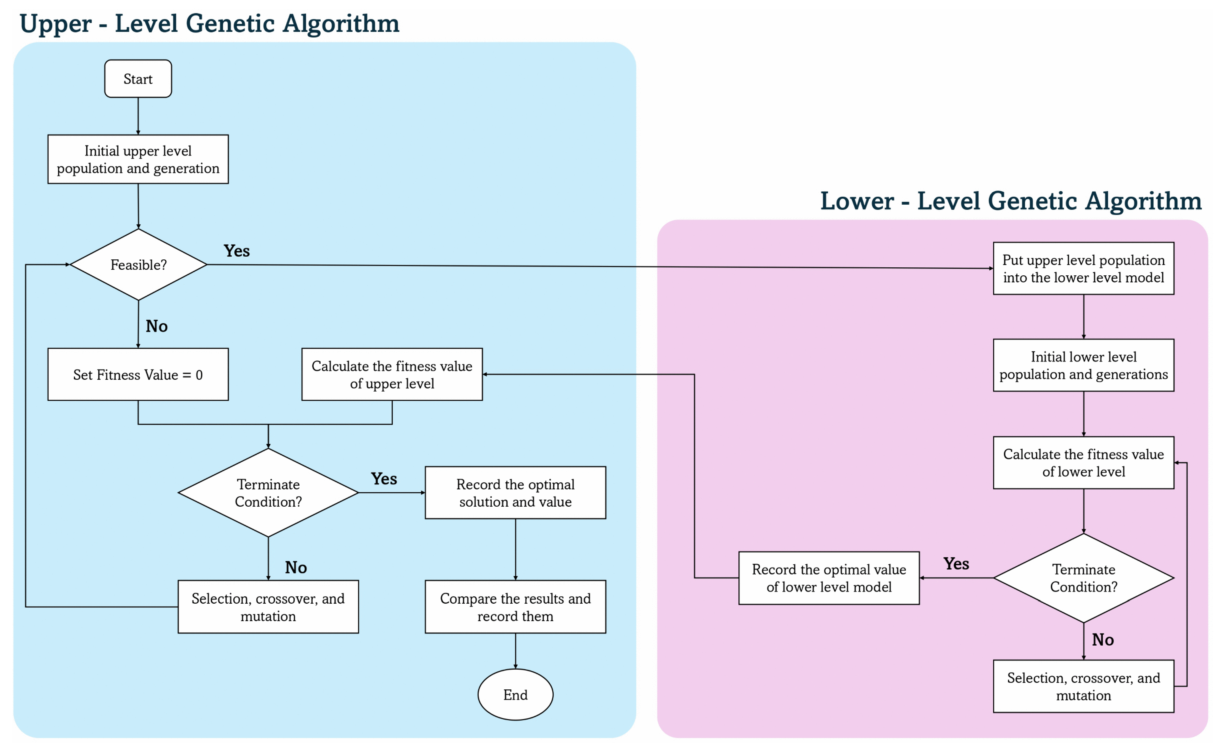
This section introduces a Two-Tier Genetic Algorithm (TT-GA), specifically designed to address the problem’s nested bi-level structure. The schematic procedure of the proposed TT-GA is illustrated in Figure 2.

The procedures employed in the TT-GA applied in this study are outlined as follows:

• The upper-level genetic algorithm commences with a uniformly initialized population, generated by encoding the upper-level decision variables. These decision variables include the production quantity $P_{ist}$, order quantity $Q_{isrt}$, and supply quantity ${SP}_{irct}$. The number of generations is then defined.
• If a chromosome is determined to be infeasible after startup, its fitness value is set to zero. The lower-level model takes the upper-level population and passes it on to the genetic algorithm that determines the appropriate ideal value for each viable chromosome.
• If the termination conditions are not met, the fitness value of the lower level is recalculated by applying the selection, crossover, and mutation operators, generating new solutions for further evaluation. The crossover operation is a single-point using a random-cut point, the mutation operator is a uniform random resetting, and the selection operator is a tournament selection. If the termination conditions are met, the optimal value and prices of the lower-level model are recorded, and the process returns to the upper level to continue the optimization.
• Following this, the upper-level genetic algorithm is executed to optimize its respective objective function. The algorithm iteratively evaluates the termination criterion; upon satisfying the maximum generation count, the optimal solutions are documented for subsequent comparative analysis. If the criterion remains unmet, the algorithm advances by applying selection, crossover, and mutation operators to evolve a new population. This cycle persists until termination, at which point the final solutions from both hierarchical levels are archived and finalized.

4.2. Two-Tier Particle Swarm Optimization Technique (TT-PSO)

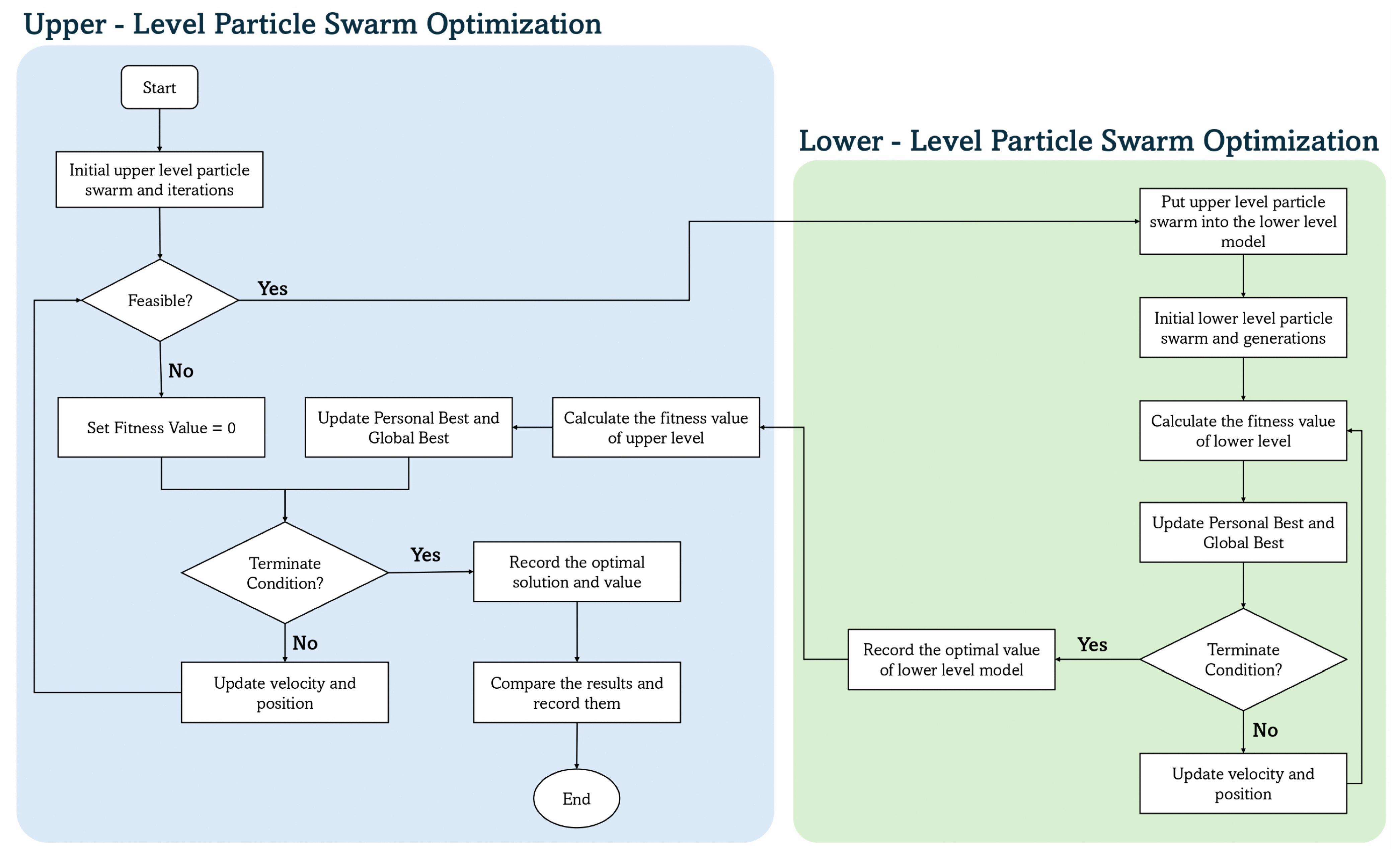
A two-tier particle swarm optimization (TT-PSO) technique is also developed to solve the bi-level problem, with its schematic architecture presented in Figure 3.

The steps taken in this research to implement the TT-PSO are explained below:

• The upper-level particle swarm optimization is initiated by uniformly initializing a swarm of particles, representing potential solutions, through the encoding of upper-level decision variables. These decision variables include the production quantity $P_{ist}$, order quantity $Q_{isrt}$, and supply quantity ${SP}_{irct}$. The algorithm then performs a set number of iterations.
• After initialization, the algorithm checks if the current solution is feasible. If it is feasible, the upper-level swarm is passed to the lower-level model. This lower-level model then runs its own particle swarm optimization to find its optimal value. Any infeasible solution is given a fitness value of zero, marking it as unacceptable. For the feasible solutions, the lower-level fitness value is updated by changing the particles’ velocities and positions. This allows the algorithm to explore a wider area of the solution space. The process then returns to the feasibility check. The algorithm repeatedly checks if the termination criteria are met. Once they are, the best solution and its corresponding lower-level value are recorded. The procedure then returns to the upper level to continue the optimization.
• The leader’s objective function is addressed using a customized particle swarm optimization approach specifically designed for the upper-level problem. The algorithm subsequently confirms whether the termination requirements have been met. Upon reaching the maximum iterations, the algorithm documents the optimal solutions and proceeds to the comparison and recording phase. Upon satisfying all termination criteria, we document, analyze, and conclude the ideal solutions for both the top and lower tiers.

5. Results and Discussion

5.1. Scenario Setting

To validate the proposed framework, a case study is conducted to illustrate the two-tier model’s characteristics and evaluate the efficacy of the applied solution methodologies, namely GA and PSO. Multiple test scenarios with different dimensions are presented, as outlined in

Table 2. The structure of the three scenarios in various dimensions.

Scenario	Plants (s)	Retailers (r)	Customers (c)
Scenario 1	3	3	3
Scenario 2	2	5	3
Scenario 3	4	5	6

. The analysis for all test problems encompassed a five-month period, $t = \left\{1,2,3,4,5\right\}$ and considered three different products, $i= \left\{1,2,3\right\}$.

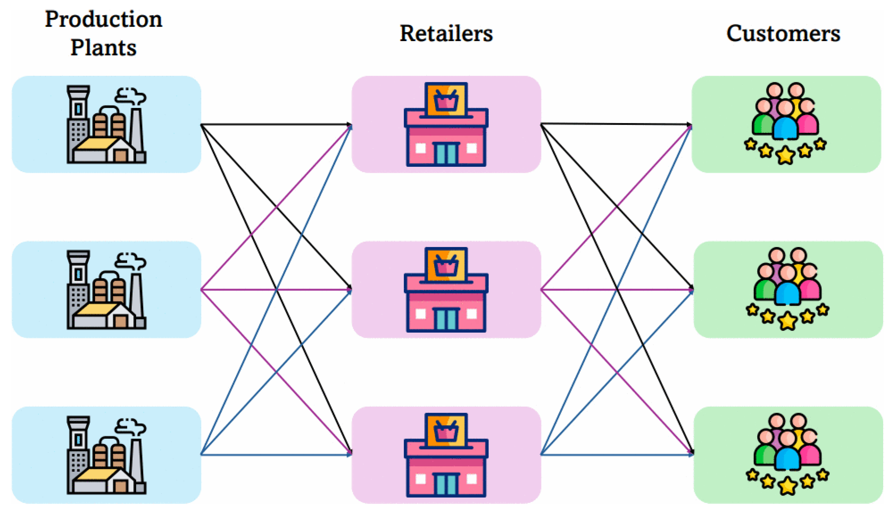
Figure 4 shows an illustrative supply chain network between production plants, retailers, and customers for Scenario 1. As shown in Figure 4, our first scenario consists of a network with three plants, $s = \left\{1,2,3\right\}$, three retailers, $r = \left\{1,2,3\right\}$, and three customers, $c = \left\{1,2,3\right\}$. The production capacity of each factory ${CAP}_{ist}$ is set at 1000 units. The inventory holding capacity of each factory ${IPM}_{st}$ is set at 6000 units. The inventory holding capacity of each retailer ${IRM}_{rt}$ is set at 9000 units. The inventory holding cost for product $i$ at each retailer $r$, ${hr}_{ir}$, is set at 0,70, 0,60, and 0,55, respectively. The unit selling price of each product $i$ from the production plant $s$ to each retailer $r$, $w_{isr}$, is set at 80, 90, and 100, respectively. The unit selling price of each product $i$ from retailer $r$ to each end customer $c$, $o_{irc}$, is set at 130, 140, and 160, respectively. The customer shortage cost of each product $i$ from retailer $r$ to each end customer $c$, ${IS}_{irc}$, is set at 40, 50, and 30, respectively.

Additionally, associated production quantity of product $i$, ${ P}_{ist}$, is required to be more than 75 units but fewer than 400 units for a plant $s$ in each period $t$. The quantity of product $i$ received from production plant $s$ to retailer $r$, $Q_{isrt}$, must be greater than 10 units but fewer than 150 units per period. The quantity of product $i$ shipped from retailer $r$ to end customer $c$, ${SP}_{irct}$, must exceed 10 units but remain below 500 units during each period $t$. The inventory capacity at each factory, ${IP}_{ist}$, is limited to 2000 units. The inventory capacity at each retailer, ${IR}_{irt}$, is limited to 3000 units. Finally, the initial inventory for each factory, $I{P}_{is0}$ and the initial inventory for each retailer, $I{R}_{ir0}$, are both set at 100 units.

5.2. Computational Results and Analysis

All computational experiments are conducted on a PC with 2.40 GHz processor. The proposed model and its corresponding solution algorithms were implemented in Python 3.11.1. The bi-level problem is solved using two metaheuristics: a Two-Tier Genetic Algorithm (TT-GA) and a Two-Tier Particle Swarm Optimization (TT-PSO). For the TT-GA, the crossover and mutation rates were configured at 0.9 and 0.2, respectively. The TT-PSO parameters were set as follows: an inertia weight of 0.7, a cognitive coefficient of 1.5, a social coefficient of 2.0, and a velocity clamping value of 10.

The selection of the mentioned key parameters is based on a combination of established practices in the metaheuristic optimization literature and preliminary experimental tuning. Specifically, the crossover and mutation rates for TT-GA (0.9 and 0.2, respectively) were chosen in accordance with commonly adopted ranges that balance exploration and exploitation in genetic algorithms. Similarly, the parameter settings for TT-PSO, including inertia weight (0.7), cognitive coefficient (1.5), and social coefficient (2.0), follow widely used configurations reported to provide stable convergence behavior across various optimization problems.

In addition, different combinations of population/particle sizes (15, 30, and 50) and generation/iteration numbers (50 and 150) were systematically evaluated. This experimental design enables an implicit sensitivity analysis by assessing algorithm performance under varying parameter scales. To ensure robustness, multiple parameter configurations were considered rather than relying on a single fixed setting, thereby reducing the risk of parameter bias. The consistency of the results across these configurations supports the stability and reliability of the proposed solution approaches. Furthermore, the results indicate that increasing population size and iteration depth generally improves solution quality, with the best performance achieved at higher parameter levels (i.e., population/particle size of 50 and 150 generations/iterations), demonstrating an effective balance between computational efficiency and solution quality.

Table 3. The computational results of the TT-GA for six different combinations in Scenario 1.

Combination No.	Population Size	Generation	Lower Fitness Value	Upper Fitness Value	Total Fitness Value
1	15	50	1,949,892.73	274,291.55	2,224,184.28
2	15	150	1,871,454.01	384,859.40	2,256,313.41
3	30	50	1,856,235.61	377,401.40	2,233,637.01
4	30	150	1,983,564.03	270,056.45	2,253,620.10
5	50	50	1,921,584.35	346,386.75	2,267,971.10
6	50	150	1,887,342.60	390,925.20	2,278,267.80

displays the TT-GA findings for various combinations, and

Table 4. The computational results of the TT-PSO for six different combinations in Scenario 1.

Combination No.	Particle Size	Iteration	Lower Fitness Value	Upper Fitness Value	Total Fitness Value
1	15	50	1,824,376.92	444,144.85	2,268,521.77
2	15	150	1,787,163.31	368,378.90	2,155,542.21
3	30	50	1,942,319.29	262,966.55	2,205,285.84
4	30	150	1,908,680.97	490,805.55	2,399,486.52
5	50	50	2,014,639.62	320,466.20	2,335,105.82
6	50	150	1,894,906.01	530,696.80	2,425,602.81

displays the TT-PSO results obtained for our Scenario 1. Table 3 and Table 4 also show the fitness values separately for the lower, upper, and total categories.

Within the framework of our problems regarding bilevel optimization, the manufacturer takes on the position of the leader, while the retailer plays the part of the follower. The higher level generally dictates the primary goal, whereas the lower level influences the solution space. The algorithm’s overall success is ultimately assessed by the optimization of the upper-level objective. Therefore, when evaluating the TT-GA and TT-PSO, we focused on achieving a greater fitness value. Among the six combinations tested using TT-GA, the one with a population size of 50 generations yielded the best upper fitness value. The TT-PSO findings indicate that the sixth combination produced the highest upper fitness value and overall fitness value among all combinations in all scenarios.

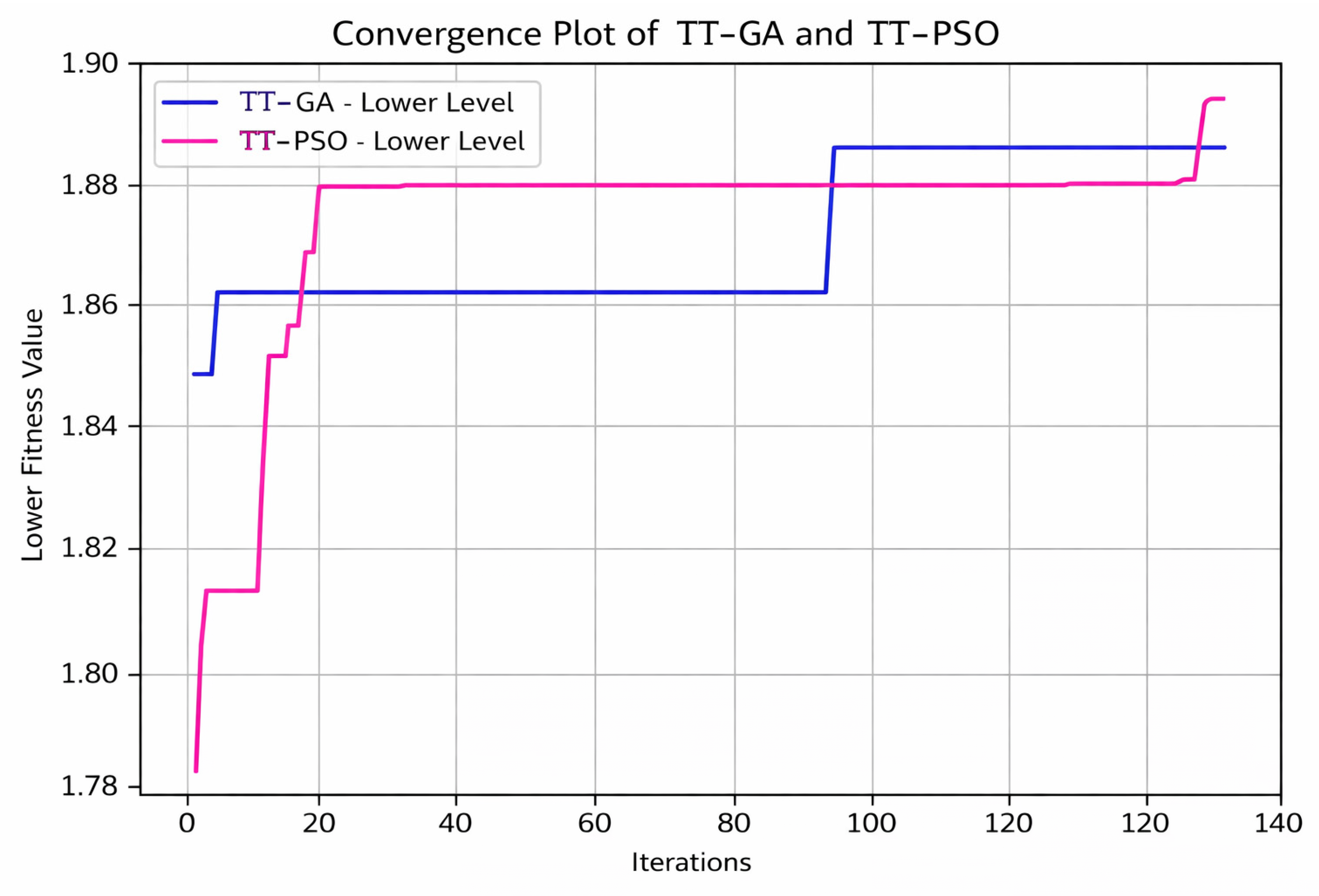
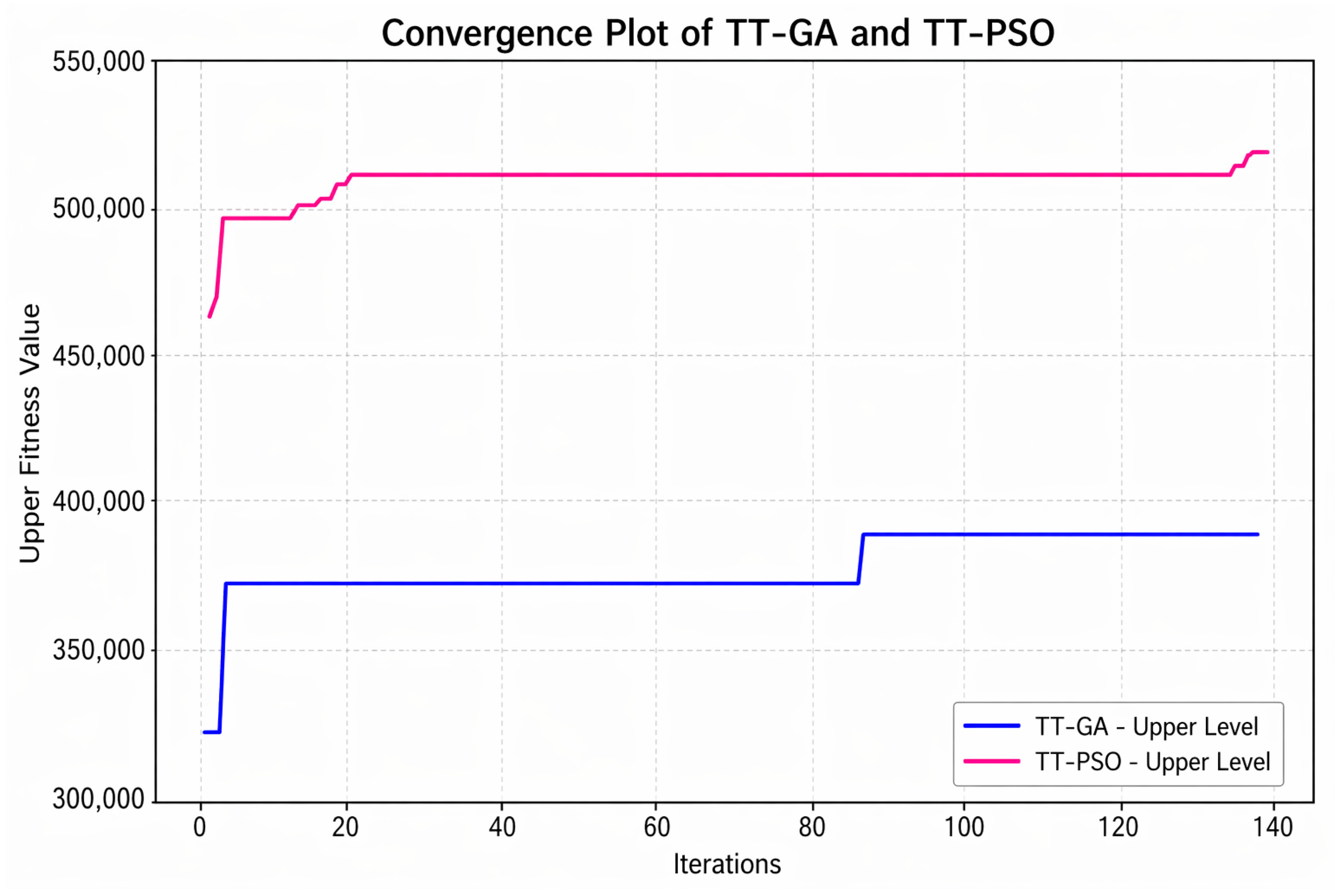
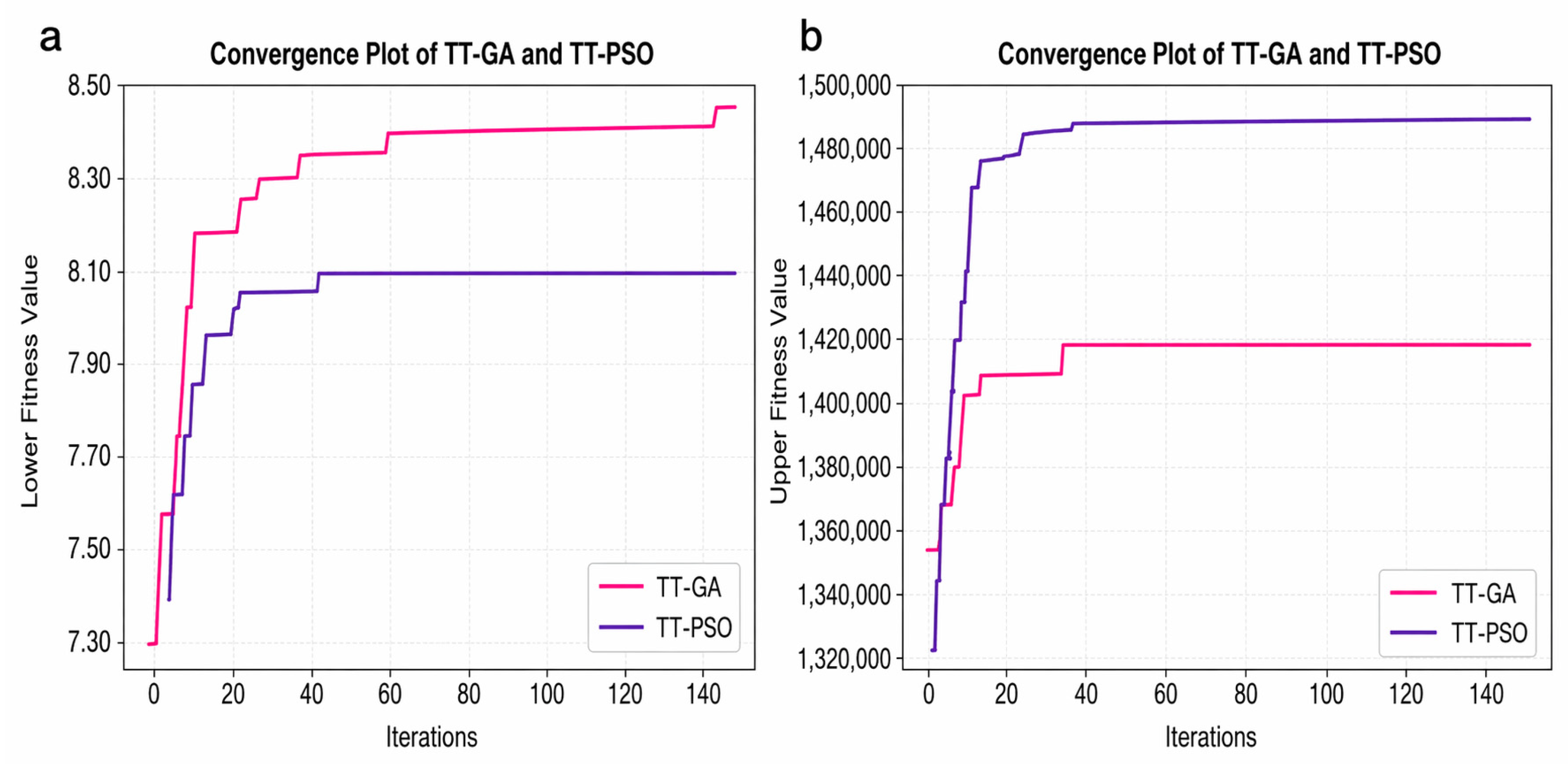
Figure 5 and Figure 6 display the convergence charts that were generated to assess the efficacy and performance of the suggested TT-GA and TT-PSO algorithms with respect to the sixth combination of parameters for Scenario 1. Here, convergence refers to the convergence of the objective function values of TT-GA and TT-PSO toward their respective optimal levels individually, rather than convergence between the objective values produced by the two algorithms. The graphs depict the variation in fitness values for both the higher and lower levels throughout iterations. The advancement of each method towards their respective optimal solutions in both tiers of the bi-level optimization can be clearly observed from the figures since the vertical axis displays the corresponding fitness values, and the horizontal axis indicates the number of iterations in each of the figures. The plots reveal that the objective function value of TT-PSO converges toward a better optimal level than that of TT-GA.

One should note that the observed differences in performance between TT-GA and TT-PSO across scenarios are due to the nature of metaheuristic optimization methods. Given their fundamentally different search mechanisms—evolutionary operators in GA and swarm-based information sharing in PSO—the convergence behavior of these algorithms is inherently problem-dependent and may vary across scenarios. As a result, even though convergence toward optimal solutions is desirable, the results obtained by TT-GA and TT-PSO do not necessarily converge to the same values or exhibit identical convergence patterns. This behavior is well documented in the literature, where comparative studies report differing convergence characteristics and solution qualities for GA and PSO depending on the problem structure [53,54,55].

Table 5. The total upper-level profit and total lower-level profit values using GA and PSO in combination 6 of Scenario 1.

		TT-GA	TT-PSO
	Upper Fitness Value	3,90,925.20	530,696.80
	Lower Fitness Value	1,887,342.60	1,894,906.01
	Total Fitness Value	2,278,267.80	2,425,602.81
Upper Level	Fixed and Production Cost	−623,823.00	−473,725.00
	Inventory Holding Cost	−2739.65	−2121.50
	Wholesale	1,032,080.00	1,021,320.00
	Transportation Cost	−14,592.15	−14,776.70
Total Upper-Level Profit		390,925.20	530,696.80
Lower Level	Inventory Holding Cost	−497.85	−1836.80
	Customer Shortage Cost	−2.00	−3.86
	Wholesale Cost	−1,032,080.00	−1,021,320.00
	Transportation Cost	−32,671.15	−34,520.90
	Sales Revenue	2,952,593.60	2,952,587.57
Total Lower-Level Profit		1,887,342.60	1,894,906.01
Total Supply Chain Profit		2,278,267.80	2,425,602.81

provides a comprehensive examination of the findings derived from the 6th combination for both the TT-GA and TT-PSO in Scenario 1. The table presents all costs for both the top and lower levels. In addition to transportation costs, fixed costs, production costs, inventory holding costs, and wholesale costs are included in the expenses for the upper level. Costs for the lower level include inventory holding costs, customer shortage costs, wholesale costs, transportation costs, and sales revenue. Upon comparison of the outcomes of the TT-GA and TT-PSO methods, it is evident that the TT-PSO approach demonstrates superior efficiency and yields more favorable results than the TT-GA method. The upper-level profit attained by the TT-PSO exhibits markedly superior performance.

It should also be noted that during the optimization of the problem with both methods, the decision variable for production quantity, $P_{ist}$, is more accurately adjusted to account for the retailer’s order quantity, $Q_{isrt}$, and uncertain demand, $d_{irct}$. As a result, decreases in the fixed and production costs and increases in the total profit are maintained.

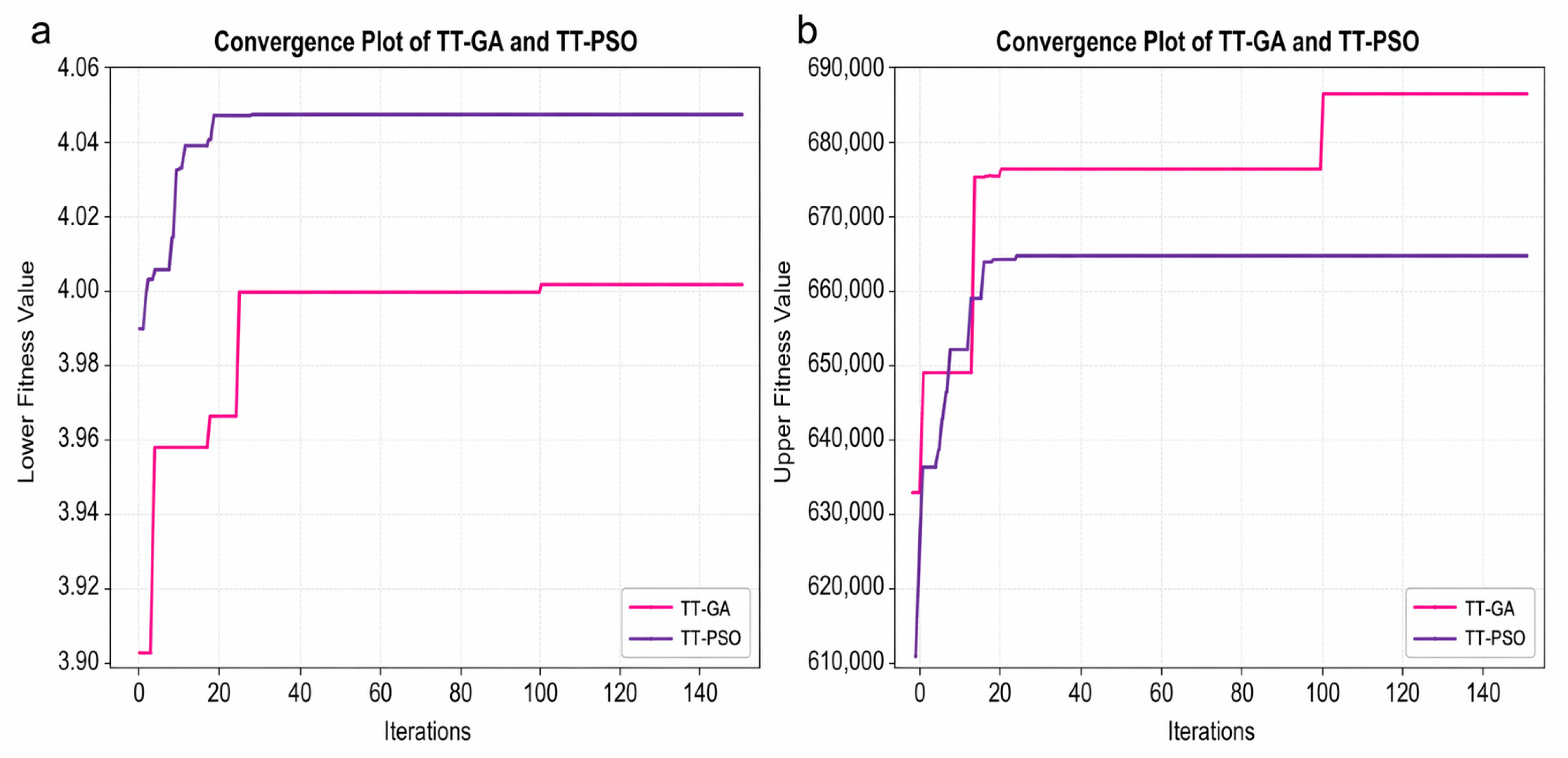
Additional analyses were conducted for Scenarios 2 and 3 to further demonstrate the practicality and effectiveness of the proposed stochastic bi-level framework. The scenarios were evaluated using the parameter settings corresponding to the sixth combination of TT-GA and TT-PSO instances in Scenario 1, ensuring consistency in the comparative analysis. The aggregated results for all scenarios are summarized in

Table 6. Computed results from the sixth combination for all scenarios.

Scenarios	GA			PSO			Profit Outperformance (%)
	Lower Fitness	Upper Fitness	Total Fitness	Lower Fitness	Upper Fitness	Total Fitness
Scenario 1	1,887,342,60	390,925.20	2,278,267.80	1,894,906.01	530,696.80	2,425,602,81	6.46 (PSO)
Scenario 2	4,071,731,72	607,088.70	4,678,820.42	4,049,644.77	664,585.60	4,714,230,37	0.76 (PSO)
Scenario 3	8,407,192,97	1,402,845.95	9,810,038.92	8,031,145.76	1,510,782.95	9,541,928,71	2.80 (GA)

, with associated convergence plots given in Figure 7 and Figure 8, providing a comprehensive basis for performance evaluation. The findings indicate that both solution approaches exhibit strong performance across varying parameter settings and problem instances, confirming their suitability for solving the proposed large-scale bi-level supply chain model. Moreover, the results highlight the robustness of the framework in capturing complex interactions and generating high-quality solutions under different demand conditions, thereby reinforcing its applicability to realistic supply chain decision-making environments. As can be seen in Table 6, TT-PSO exhibits enhanced performance regarding upper-level outcomes for all three scenarios. Overall profit outperformance values of the algorithms are also given in Table 6 for comparison. TT-PSO outperformed TT-GA in Scenarios 1 and 2 with profit improvements of 6.46% and 0.76%, respectively, whereas TT-GA achieved superior performance in Scenario 3 with a 2.80% profit improvement.

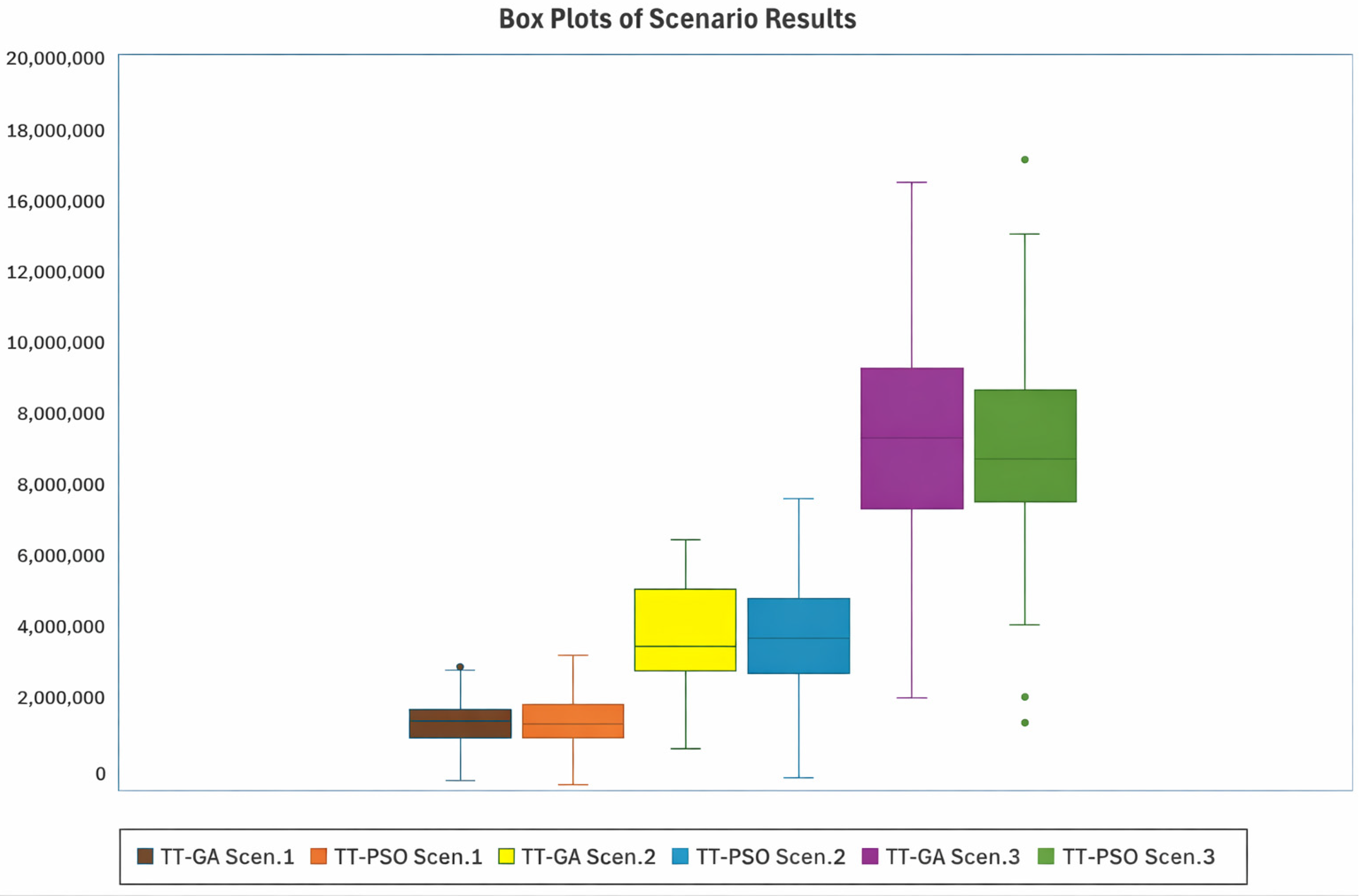
Finally, we have conducted additional experiments to better evaluate the performance, stability, and variability of the proposed model through the applied algorithms TT-GA and TT-PSO and generated box plots of the resulting total fitness values obtained from 50 independent runs for both algorithms as shown in Figure 9. The box plots are provided for all three scenarios considered, enabling a comprehensive evaluation of the proposed model, as well as facilitating the identification of potential outliers.

6. Conclusions

This study developed a comprehensive stochastic bi-level optimization framework for a two-tier, three-echelon supply chain operating under demand uncertainty, enabling a more realistic representation of the inherent complexity of real-world supply chain networks. The proposed model captures leader–follower interactions among multiple decision-makers, including plant owners (manufacturers), retailers, and end customers, and represents the flow of multiple products across the supply chain network. The framework jointly determines optimal production and allocation quantities while simultaneously maximizing total profit at both upper and lower levels, accounting for fixed costs, production costs, inventory holding costs, transportation costs, wholesale prices, and uncertain demand.

This joint optimization is particularly significant, as it ensures that decisions made at the production level are aligned with downstream allocation and retail strategies, thereby reducing inefficiencies arising from decentralized decision-making. By explicitly integrating these interdependent decisions within a unified framework, the model enhances coordination across the supply chain and enables more balanced and globally optimal outcomes. As a result, the proposed approach not only improves solution quality in terms of profitability but also strengthens the consistency and robustness of decisions under uncertainty. This highlights the practical value of the framework as a decision-support tool for managing complex supply chain systems where coordination between hierarchical levels is critical for achieving superior overall performance.

To solve the resulting large-scale nonlinear bi-level problem, two tailored metaheuristic solution approaches—TT-GA and TT-PSO—were applied and evaluated under three test scenarios. The comparative results demonstrate that TT-PSO outperformed TT-GA in Scenarios 1 and 2, achieving overall profit improvements of 6.46% and 0.76%, respectively. In contrast, TT-GA achieved superior performance in Scenario 3, yielding a 2.80% improvement in overall profit. These findings confirm the effectiveness of the proposed framework and highlight the complementary strengths of the two-tier metaheuristic approaches for solving complex decentralized supply chain problems under demand uncertainty. From a managerial perspective, the proposed framework enables coordinated pricing and allocation decisions under demand uncertainty, contributing to higher overall profitability across both production and retail levels of the supply chain.

Several promising directions for future research can be identified. (1) The proposed framework can be extended to incorporate additional supply chain participants, such as distributors, suppliers, and remanufacturing facilities, to capture more complex network structures. (2) Safety stock policies and penalty costs for exceeding safety stock thresholds can be integrated to enhance inventory control effectiveness. (3) Additional sources of uncertainty, such as price volatility and supply-side uncertainty, may be incorporated alongside demand uncertainty. (4) Alternative scenario-based methods for modeling demand uncertainty can be explored to improve solution robustness. (5) Sustainability considerations, including environmental objectives and emission constraints, can be integrated into the optimization framework. (6) A broader comparative analysis involving relevant algorithms (i.e., Jaya [56], Butterfly [57], Tree-seed [58]) for addressing the complex problem under consideration would constitute a valuable extension to obtain deeper insights into the relative strengths and limitations of alternative approaches. Moreover, incorporating dynamic learning mechanisms or real-time data analytics into the decision-making process may further enhance the adaptability of the proposed framework in highly volatile supply chain environments.

References

1. Lee, H.L. The Triple-A Supply Chain. Harv. Bus. Rev. 2004, 82, 102–112. [Google Scholar]
2. Christopher, M. Logistics and Supply Chain Management, 5th ed.; Pearson Education Limited: Harlow, UK, 2016. [Google Scholar]
3. Robles, J.O.; Azzaro-Pantel, C.; Aguilar-Lasserre, A. Optimization of a hydrogen supply chain network design under demand uncertainty by multi-objective genetic algorithms. Comput. Chem. Eng. 2020, 140, 106853. [Google Scholar] [CrossRef]
4. Mekamcha, K.; Souier, M.; Bessenouci, H.N.; Bennekrouf, M. Two metaheuristic approaches for solving the travelling salesman problem: An Algerian waste collection case. Oper. Res. 2021, 21, 1641–1661. [Google Scholar] [CrossRef]
5. Toaza, B.; Esztergár-Kiss, D. A review of metaheuristic algorithms for solving TSP-based scheduling optimization problems. Appl. Soft Comput. 2023, 148, 110908. [Google Scholar] [CrossRef]
6. Capobianco, G.; D’Ambrosio, C.; Pavone, L.; Raiconi, A.; Vitale, G.; Sebastiano, F. A hybrid metaheuristic for the knapsack problem with forfeits. Soft Comput. 2022, 26, 749–762. [Google Scholar] [CrossRef]
7. Scherer, M.E.; Hill, R.R.; Lunday, B.J.; Cox, B.A.; White, E.D. Applying instance space analysis for metaheuristic selection to the 0–1 multidemand multidimensional knapsack problem. Comput. Oper. Res. 2024, 170, 106747. [Google Scholar] [CrossRef]
8. Ding, R.; Deng, B.; Li, W. Metaheuristic algorithms for the generalized extensible bin packing problem with overload cost. IEEE Access 2022, 10, 124858–124873. [Google Scholar] [CrossRef]
9. Grandcolas, S.; Pain-Barre, C. A hybrid metaheuristic for the two-dimensional strip packing problem. Ann. Oper. Res. 2022, 309, 79–102. [Google Scholar] [CrossRef]
10. Đurasević, M.; Jakobović, D. Heuristic and metaheuristic methods for the parallel unrelated machines scheduling problem: A survey. Artif. Intell. Rev. 2023, 56, 3181–3289. [Google Scholar] [CrossRef]
11. Barbalho, T.J.; Santos, A.C.; Aloise, D.J. Metaheuristics for the work-troops scheduling problem. Int. Trans. Oper. Res. 2023, 30, 892–914. [Google Scholar] [CrossRef]
12. Camacho-Vallejo, J.F.; Corpus, C.; Villegas, J.G. Metaheuristics for bilevel optimization: A comprehensive review. Comput. Oper. Res. 2024, 161, 106410. [Google Scholar] [CrossRef]
13. Huang, P.Q.; Zhang, Q.; Wang, Y. Bilevel optimization via collaborations among lower-level optimization tasks. IEEE Trans. Evol. Comput. 2023, 27, 1837–1850. [Google Scholar] [CrossRef]
14. Talbi, E.G. A taxonomy of metaheuristics for bilevel optimization. In Metaheuristics for Bilevel Optimization; Springer: Berlin/Heidelberg, Germany, 2013; pp. 1–39. [Google Scholar] [CrossRef]
15. Saif-Eddine, A.S.; El-Beheiry, M.M.; El-Kharbotly, A.K. An improved genetic algorithm for optimizing total supply chain cost in inventory location routing problem. Ain Shams Eng. J. 2019, 10, 63–76. [Google Scholar] [CrossRef]
16. Soleimani, H.; Kannan, G. A hybrid particle swarm optimization and genetic algorithm for closed-loop supply chain network design in large-scale networks. Appl. Math. Model. 2015, 39, 3990–4012. [Google Scholar] [CrossRef]
17. Sun, J.; Chen, Z.; Chen, Z.; Li, X. Robust optimization of a closed-loop supply chain network based on an improved genetic algorithm in an uncertain environment. Comput. Ind. Eng. 2024, 189, 109997. [Google Scholar] [CrossRef]
18. Zhang, X.; Sun, S.; Yao, J.; Fang, W.; Qian, P. Multi-population genetic algorithm with crowding-based local search for fuzzy multi-objective supply chain configuration. Swarm Evol. Comput. 2024, 91, 101698. [Google Scholar] [CrossRef]
19. Chang, C.K.; Cheng, D.W. A Genetic Algorithm-Based Optimization Method for Ordered Escape Routing in BGA PCBs Under Non-Crossing and Single-Capacity Constraints. Appl. Sci. 2026, 16, 2010. [Google Scholar] [CrossRef]
20. Chen, Y.H.; Wang, H.W.; Tsai, C.H.; Wu, C.H. A genetic algorithm for tool-constrained scheduling with dynamic expedited orders in smart manufacturing. J. Ind. Manag. Optim. 2026, 22, 182–213. [Google Scholar] [CrossRef]
21. Che, Z.H. A particle swarm optimization algorithm for solving unbalanced supply chain planning problems. Appl. Soft Comput. 2012, 12, 1279–1287. [Google Scholar] [CrossRef]
22. Gao, Q.; Xu, H.; Li, A. The analysis of commodity demand prediction in supply chain networks based on particle swarm optimization. J. Comput. Appl. Math. 2022, 400, 113760. [Google Scholar] [CrossRef]
23. Hachaichi, Y.; Khedr, A.E.; Idrees, A.M. A proposed feature selection particle swarm optimization adaptation for intelligent logistics: A supply chain backlog elimination framework. Comput. Mater. Contin. 2024, 79, 048929. [Google Scholar] [CrossRef]
24. Shami, T.M.; El-Saleh, A.A.; Alswaitti, M.; Al-Tashi, Q.; Mirjalili, S.; Faris, H. Particle swarm optimization: A comprehensive survey. IEEE Access 2022, 10, 10031–10061. [Google Scholar] [CrossRef]
25. Kadadevaramath, R.S.; Chen, J.C.; Shankar, B.L.; Rameshkumar, K. Application of particle swarm intelligence algorithms in supply chain network architecture optimization. Expert Syst. Appl. 2012, 39, 10160–10176. [Google Scholar] [CrossRef]
26. Kennedy, J.; Eberhart, R. Particle swarm optimization. In Proceedings of the ICNN’95—International Conference on Neural Networks; IEEE: New York, NY, USA, 1995; Volume 4, pp. 1942–1948. [Google Scholar] [CrossRef]
27. Liu, L.; Ouyang, J.; Nian, G.; Zhu, Y.; Liang, N. In Situ Stress Inversion in a Pumped-Storage Power Station Based on the PSO-SVR Algorithm. Appl. Sci. 2026, 16, 1101. [Google Scholar] [CrossRef]
28. Guan, J.; Ye, S.; Yi, W. MSCPSO: A multi-strategy cooperative particle swarm optimization algorithm for UAV path planning. Expert Syst. Appl. 2026, 310, 131034. [Google Scholar] [CrossRef]
29. Beck, Y.; Ljubić, I.; Schmidt, M. A survey on bilevel optimization under uncertainty. Eur. J. Oper. Res. 2023, 311, 401–426. [Google Scholar] [CrossRef]
30. Sinha, A.; Malo, P.; Deb, K. A review on bilevel optimization: From classical to evolutionary approaches and applications. IEEE Trans. Evol. Comput. 2017, 22, 276–295. [Google Scholar] [CrossRef]
31. Kasimoglu, F.; Akgün, İ. Project management in a competitive environment: Interdicting a CPM-based project and its implications. RAIRO—Oper. Res. 2021, 55, S365–S384. [Google Scholar] [CrossRef]
32. Kasimoğlu, F.; Bayeğ, S.; Utku, D.H. Analyzing the vulnerabilities in a transshipment network: A bilevel programming approach. IEEE Access 2023, 11, 57635–57651. [Google Scholar] [CrossRef]
33. Zenhom, Z.M.; Aleem, S.H.A.; El Zahab, E.E.D.A.; Ali, Z.M.; Almalaq, A.; Boghdady, T.A. Synergistic hierarchical bi-level optimization of demand response programs and smart inverter Volt/Var control for maximizing hosting capacity of power systems with renewable-based distributed generators. IEEE Access 2025, 13, 15390–15409. [Google Scholar] [CrossRef]
34. Khanduzi, R.; Sadati, İ.; Akbari, V. A bilevel hierarchical covering model to protect a healthcare network against failures. Oper. Res. 2024, 24, 61. [Google Scholar] [CrossRef]
35. Yan, X.; Wu, Z.; Wang, H. Network noise control under speed limit strategies using an improved bilevel programming model. Transp. Res. Part D Transp. Environ. 2023, 121, 103805. [Google Scholar] [CrossRef]
36. Yin, L.; Fang, Z.; Li, K.; Chen, J.; Fan, N.; Li, M. A Bi-Level Intelligent Control Framework Integrating Deep Reinforcement Learning and Bayesian Optimization for Multi-Objective Adaptive Scheduling in Opto-Mechanical Automated Manufacturing. Appl. Sci. 2026, 16, 732. [Google Scholar] [CrossRef]
37. Jiang, P.; Guo, S.; Luo, X. Bi-level collaborative optimization for medical consumable order splitting and reorganization considering multi-dimensional and multi-scale characteristics. Appl. Sci. 2025, 15, 7627. [Google Scholar] [CrossRef]
38. Hansen, P.; Jaumard, B.; Savard, G. New branch-and-bound rules for linear bilevel programming. SIAM J. Sci. Stat. Comput. 1992, 13, 1194–1217. [Google Scholar] [CrossRef]
39. Buchheim, C. Bilevel linear optimization belongs to NP and admits polynomial-size KKT-based reformulations. Oper. Res. Lett. 2023, 51, 618–622. [Google Scholar] [CrossRef]
40. Cheraghalipour, A.; Paydar, M.M.; Hajiaghaei-Keshteli, M. Designing and solving a bi-level model for rice supply chain using evolutionary algorithms. Comput. Electron. Agric. 2019, 162, 651–668. [Google Scholar] [CrossRef]
41. Amirtaheri, O.; Zandieh, M.; Dorri, B.; Motameni, A.R. A bi-level programming approach for production–distribution supply chain problem. Comput. Ind. Eng. 2017, 110, 527–537. [Google Scholar] [CrossRef]
42. Kwong, C.K.; Xia, Y.; Chan, C.Y.; Ip, W.H. Incorporating contracts with retailers into product line extension using Stackelberg game and bi-level genetic algorithms. Comput. Ind. Eng. 2021, 151, 106976. [Google Scholar] [CrossRef]
43. Chalmardi, M.K.; Camacho-Vallejo, J.F. A bi-level programming model for sustainable supply chain network design that considers incentives for using cleaner technologies. J. Clean. Prod. 2019, 213, 1035–1050. [Google Scholar] [CrossRef]
44. Haque, M.; Paul, S.K.; Sarker, R.; Essam, D. Managing decentralized supply chains using bilevel with Nash game approach. J. Clean. Prod. 2020, 266, 121865. [Google Scholar] [CrossRef]
45. Cui, Y.Y.; Guan, Z.; Saif, U.; Zhang, L.; Zhang, F.; Mirza, J. Closed-loop supply chain network problem with uncertainty in demand and returned products: Genetic artificial bee colony algorithm approach. J. Clean. Prod. 2017, 162, 717–742. [Google Scholar] [CrossRef]
46. Yin, S.; Nishi, T.; Grossmann, I.E. Optimal quantity discount coordination for supply chain optimization with one manufacturer and multiple suppliers under demand uncertainty. Int. J. Adv. Manuf. Technol. 2015, 76, 1173–1184. [Google Scholar] [CrossRef]
47. Gupta, A.; Maranas, C.D.; McDonald, C.M. Mid-term supply chain planning under demand uncertainty: Customer demand satisfaction and inventory management. Comput. Chem. Eng. 2000, 24, 2613–2621. [Google Scholar] [CrossRef]
48. Petkov, S.B.; Maranas, C.D. Multiperiod planning and scheduling of multiproduct batch plants under demand uncertainty. Ind. Eng. Chem. Res. 1997, 36, 4864–4881. [Google Scholar] [CrossRef]
49. Nishi, T.; Yoshida, O. Optimization of multi-period bilevel supply chains under demand uncertainty. Procedia CIRP 2016, 41, 508–513. [Google Scholar] [CrossRef][Green Version]
50. Hosseini-Motlagh, S.M.; Govindan, K.; Nematollahi, M.; Jokar, A. An adjustable bi-level wholesale price contract for coordinating a supply chain under scenario-based stochastic demand. Int. J. Prod. Econ. 2019, 214, 175–195. [Google Scholar] [CrossRef]
51. Nezamoddini, N.; Gholami, A. Integrated genetic algorithm and artificial neural network. In Proceedings of the 2019 IEEE International Conference on Computational Science and Engineering and IEEE International Conference on Embedded and Ubiquitous Computing; IEEE: New York, NY, USA, 2019; pp. 260–262. [Google Scholar] [CrossRef]
52. Setak, M.; Feizizadeh, F.; Tikani, H.; Ardakani, E.S. A bi-level stochastic optimization model for reliable supply chains in competitive environments: Hybridizing exact methods and genetic algorithm. Appl. Math. Model. 2019, 75, 310–332. [Google Scholar] [CrossRef]
53. Papazoglou, G.; Biskas, P. Review and Comparison of Genetic Algorithm and Particle Swarm Optimization in the Optimal Power Flow Problem. Energies 2023, 16, 1152. [Google Scholar] [CrossRef]
54. Dwivedi, A.; Madaan, J.; Chan, F.T.S.; Dalal, M. A Comparative Study of GA and PSO Approach for Cost Optimisation in Product Recovery Systems. Int. J. Prod. Res. 2023, 61, 1283–1297. [Google Scholar] [CrossRef]
55. Bouchakour, A.; Zarour, L.; Bessous, N.; Bechouat, M.; Borni, A.; Zaghba, L.; Rabehi, A.; Alwabli, A.; El-Abd, M.; Ghoneim, S.S.M. MPPT Algorithm Based on Metaheuristic Techniques (PSO & GA) dedicated to improve wind energy water pumping system performance. Sci. Rep. 2024, 14, 17891. [Google Scholar] [CrossRef] [PubMed]
56. Zhang, G.; Wan, C.; Xie, L.; Xue, S. Structural damage identification with output-only measurements using modified Jaya algorithm and Tikhonov regularization method. Smart Struct. Syst. 2023, 31, 229–245. [Google Scholar] [CrossRef]
57. Zhou, H.; Zhang, G.; Wang, X.; Ni, P.; Zhang, J. Structural identification using improved butterfly optimization algorithm with adaptive sampling test and search space reduction method. In Structures; Elsevier: Amsterdam, The Netherlands, 2021; Volume 33, pp. 2121–2139. [Google Scholar] [CrossRef]
58. Kiran, M.S. TSA: Tree-Seed Algorithm for Continuous Optimization. Expert Syst. Appl. 2015, 42, 6686–6698. [Google Scholar] [CrossRef]
Figure 1. A two-tier supply chain network structured with three echelons.
Applsci 16 03817 g001
Figure 3. Flowchart of the proposed TT-PSO.
Applsci 16 03817 g003
Figure 4. An illustrative supply chain network for Scenario 1.
Applsci 16 03817 g004
Figure 5. The lower-level convergence plot of the TT-GA and TT-PSO in combination 6 of Scenario 1.
Applsci 16 03817 g005
Figure 6. The upper-level convergence plot of the TT-GA and TT-PSO in combination 6 of Scenario 1.
Applsci 16 03817 g006
Figure 7. The lower (a) and upper (b) level convergence plots of the TT-GA and TT-PSO in combination 6 of Scenario 2.
Applsci 16 03817 g007
Figure 8. The lower (a) and upper (b) level convergence plots of the TT-GA and TT-PSO in combination 6 of Scenario 3.
Applsci 16 03817 g008
Figure 9. Box plots of scenario results for 50 independent runs.
Applsci 16 03817 g009